Large Complex Correlated Wishart Matrices:
The Pearcey Kernel and Expansion at the Hard Edge.

Abstract

We study the eigenvalue behaviour of large complex correlated Wishart matrices near an interior point of the limiting spectrum where the density vanishes (cusp point), and refine the existing results at the hard edge as well. More precisely, under mild assumptions for the population covariance matrix, we show that the limiting density vanishes at generic cusp points like a cube root, and that the local eigenvalue behaviour is described by means of the Pearcey kernel if an extra decay assumption is satisfied. As for the hard edge, we show that the density blows up like an inverse square root at the origin. Moreover, we provide an explicit formula for the $1/N$ correction term for the fluctuation of the smallest random eigenvalue.

AMS 2000 subject classification: Primary 15A52, Secondary 15A18, 60F15.
Key words and phrases: Large random matrices, Wishart matrix, Pearcey kernel, Bessel kernel.

1 Introduction

Empirical covariance matrices are natural random matrix models in applied mathematics and their study goes back at least to the work of Wishart [wishart-1928]. In the large dimensional regime, where both the size of the observations and of the sample go to infinity at the same speed, Marčenko and Pastur provided in the seminal paper [mar-and-pas-67] the first description of the limiting spectral distribution for such matrices, see also [silverstein-choi-1995]. For instance, this limiting distribution has a continuous density on $(0,\infty)$; its support is compact if the spectral norm of the population covariance matrix is bounded; it may include the origin and may also present several connected components.

Afterwards, attention turned to the local behaviour of the random eigenvalues near points of interest in the limiting spectrum, like positive endpoints (soft edges), see e.g. [Jo, Joh01, 4, 15, HHN-preprint], interior points were the density vanishes (cusp points) [Mo2], or the origin when it belongs to the spectrum (hard edge) [16, HHN-preprint]. Complex correlated Wishart matrices, namely covariance matrices with complex Gaussian entries, play a particular role in such investigations since their random eigenvalues form a determinantal point process. Indeed, for determinantal point processes, a local asymptotic analysis can often be performed by using tools from complex analysis such as saddle point analysis or Riemann-Hilbert techniques. In the more general setting of non-necessarily Gaussian entries, one then typically shows that the local behaviours are the same as in the Gaussian case by comparison or interpolation methods, see e.g. [knowles-yin-2014-preprint, LS14].

For complex correlated Wishart matrices, a fairly complete picture of the local fluctuations at every edges of the limiting spectrum has been obtained in the recent work [HHN-preprint], provided that a regularity condition is satisfied. This condition essentially warrants the local fluctuations to follow the usual laws from random matrix theory. For instance, if one considers a soft edge of the limiting spectrum, then this regularity condition ensures that the limiting density vanishes like a square root at the edge, and the fluctuations of the associated extremal eigenvalues follow the Tracy-Widom law involving the Airy kernel. As for the hard edge, when it is present, the fluctuations are described instead by means of the Bessel kernel.

The aim of this work is twofold. First, we investigate the local behaviour of the eigenvalues near a cusp point which satisfies the regularity condition: We show that the limiting density vanishes like a cube root near the cusp point (hence justifying the name) and, under an extra assumption on the decay of a speed parameter, we establish that the eigenvalues local fluctuations near the cusp point are described by means of the Pearcey kernel.

Our second contribution is to strengthen the results of [HHN-preprint] concerning the local analysis at the hard edge: We show that the density behaves like an inverse square root near the origin, and we provide an explicit formula for the next-order correction term for the fluctuations. This last result is motivated by the recent work [13] by Edelman, Guionnet and Péché where they conjecture a precise formula for the next-order term for the non-correlated Wishart matrix, a conjecture then proven right by Bornemann [7] and Perret and Schehr [PS], with different strategies. Our result hence extends this formula, with an alternative proof, to the more general setting of correlated Wishart matrices.

The reader interested in a pedagogical overview on the results from [HHN-preprint] and the present work may have a look at the survey [HHN-esaim-preprint]; it also contains further information on the matrix model and lists some open problems.

Let us also stress that, at the technical level, the study of this matrix model shares similar features with the study of the additive perturbation of a GUE random matrix [10], and random Gelfand-Tsetlin patterns [11, 12], although each model ultimately brings up its own share of technicalities.

We provide precise statements for our results in Section 2, and then prove the results on the density behaviour in Section 3, the cusp point fluctuations in Section 4, and the expansion at the hard edge in Section 5.

Acknowledgements.

The authors are pleased to thank Folkmar Bornemann, Antti Knowles and Anthony Metcalfe for fruitful discussions. During this work, AH was supported by the grant KAW 2010.0063 from the Knut and Alice Wallenberg Foundation. The work of WH and JN was partially supported by the program “modèles numériques” of the French Agence Nationale de la Recherche under the grant ANR-12-MONU-0003 (project DIONISOS). Support of Labex BÉZOUT from Université Paris Est is also acknowledged.

2 Statement of the main results

2.1 The matrix model and assumptions

The random matrix model of interest here is the $N\times N$ matrix

$${\mathbf{M}}_{N}=\frac{1}{N}{\bf X}_{N}{\bf\Sigma}_{N}{\bf X}_{N}^{*}$$ (2.1)

where ${\bf X}_{N}$ is a $N\times n$ matrix with independent and identically distributed (i.i.d.) entries with zero mean and unit variance, and ${\bf\Sigma}_{N}$ is a $n\times n$ deterministic positive definite Hermitian matrix. The random matrix $\mathbf{M}_{N}$ thus has $N$ non-negative eigenvalues, but which may be of different nature: The smallest $N-\min(n,N)$ eigenvalues are deterministic and all equal to zero, whereas the other $\min(n,N)$ eigenvalues are random. The problem is then to describe the asymptotic behaviour of the random eigenvalues of $\mathbf{M}_{N}$, as the size of the matrix grows to infinity. As for the asymptotic regime of interest, we let both the number of rows and columns of ${\bf X}_{N}$ grow to infinity at the same speed: We assume $n=n(N)$ and $n,N\to\infty$ so that

$$\lim_{N\rightarrow\infty}\frac{n}{N}=\gamma\in(0,\infty)\ .$$ (2.2)

This regime will be simply referred to as $N\to\infty$ in the sequel.

Let us mention that the $n\times n$ random covariance matrix

$$\widetilde{\mathbf{M}}_{N}=\frac{1}{N}{\bf\Sigma}_{N}^{1/2}{\bf X}_{N}^{*}{\bf X}_{N}{\bf\Sigma}_{N}^{1/2}\ ,$$

which is also under consideration, has exactly the same random eigenvalues as $\mathbf{M}_{N}$, and hence results on the random eigenvalues can be carried out from one model to the other immediately.

Our first assumption is that the entries of $\boldsymbol{X}_{N}$ are complex Gaussian. As we shall state later on, this assumption is fundamental for our local eigenvalue behaviour analysis, but not for our results on the limiting density behaviour, see Remark 2.3.

Assumption 1.

The entries of $\mathbf{X}_{N}$ are i.i.d. standard complex Gaussian random variables.

Considering now the matrix $\mathbf{\Sigma}_{N}$, we denote by $0<\lambda_{1}\leqslant\cdots\leqslant\lambda_{n}$ its eigenvalues and by

$$\nu_{N}=\frac{1}{n}\sum_{j=1}^{n}\delta_{\lambda_{j}}$$ (2.3)

its spectral measure. We also make the following assumption.

Assumption 2.

1. For $N$ large enough, the eigenvalues of $\mathbf{\Sigma}_{N}$ stay in a compact subset of $(0,+\infty)$ independent of $N$, i.e.

   $$0\ <\ \liminf_{N\rightarrow\infty}\lambda_{1}\ ,\quad\sup_{N}\lambda_{n}\ <\ +\infty.$$ (2.4)

2. The measure $\nu_{N}$ weakly converges towards a limiting probability measure $\nu$ as $N\rightarrow\infty$, namely

   $$\frac{1}{n}\sum_{j=1}^{n}f(\lambda_{j})\xrightarrow[N\to\infty]{}\int f(x)\nu({\rm d}x)$$ (2.5)

   for every bounded and continuous function $f$.

Again, Assumption 2(a) is necessary for our results on the local eigenvalue behaviour, but our results on the limiting density behaviour require a weaker assumption, see Remark 2.3.

We now turn to the description of the asymptotic eigenvalue distribution.

2.2 Limiting eigenvalue distribution

Consider the empirical distribution of the eigenvalues $(x_{i})$ of ${\bf M}_{N}$, namely

$$\mu_{N}=\frac{1}{N}\sum_{i=1}^{N}\delta_{x_{i}}\,.$$

Since the seminal work of Marčenko and Pastur [mar-and-pas-67], it is known that this measure almost surely (a.s.) converges weakly towards a limiting probability measure $\mu$ with compact support, provided that Assumption 2 holds true:

$$\frac{1}{N}\sum_{i=1}^{N}f(x_{i})\xrightarrow[N\to\infty]{a.s.}\int f(x)\mu({\rm d}x)$$ (2.6)

for every bounded and continuous function $f$. As a probability measure, $\mu$ is characterized by its Cauchy-Stieltjes transform, which is the holomorphic function defined by

$$m(z)=\int\frac{1}{z-\lambda}\,\mu({\rm d}\lambda),\qquad z\in\mathbb{C}_{+}=\big{\{}z\in\mathbb{C}:\;{\mathfrak{Im}}(z)>0\big{\}}\,.$$ (2.7)

Marčenko and Pastur proved that $m(z)$ is the unique solution $m\in\mathbb{C}_{-}=\{z\in\mathbb{C}:\;{\mathfrak{Im}}(z)<0\}$ of the fixed-point equation

$$m=\left(z-\gamma\int\frac{\lambda}{1-m\lambda}\nu({\rm d}\lambda)\right)^{-1},$$ (2.8)

where we recall that $\gamma$ has been introduced in (2.2) and $\nu$ is the weak limit of $\nu_{N}$, see (2.5). Thanks to this equation, Silverstein and Choi then showed in [silverstein-choi-1995] that $\mu(\{0\})=(1-\gamma)^{+}$ and $\lim_{z\in\mathbb{C}_{+}\to x}m(z)\equiv m(x)$ exists for every $x\in\mathbb{R}^{*}=\mathbb{R}-\{0\}$. Consequently, the function $m(z)$ can be continuously extended to $\mathbb{C}_{+}\cup\mathbb{R}^{*}$ and, furthermore, $\mu$ has a density on $(0,\infty)$ given by

$$\rho(x)=-\frac{1}{\pi}{\mathfrak{Im}}\,(m(x))\,.$$ (2.9)

We therefore have the representation

$$\mu({\rm d}x)=\left(1-\gamma\right)^{+}\,\delta_{0}+\rho(x){\rm d}x\ .$$ (2.10)

They also obtained that $\rho(x)$ is real analytic wherever it is positive, and they moreover characterized the (compact) support $\operatorname{Supp}(\rho)$ of the measure $\rho(x){\rm d}x$ by building on ideas from [mar-and-pas-67]. More specifically, one can see that the function $m(z)$ has an explicit inverse (for the composition law) on $m(\mathbb{C}_{+})$ given by

$$g(m)=\frac{1}{m}+\gamma\int\frac{\lambda}{1-m\lambda}\,\nu({\rm d}\lambda)\ .$$ (2.11)

If we introduce the open subset of the real line

$$D=\bigl{\{}x\in\mathbb{R}:\ x\neq 0,\;x^{-1}\notin\operatorname{Supp}(\nu)\bigr{\}}\ ,$$ (2.12)

then the map $g$ analytically extends to $\mathbb{C}_{+}\cup\mathbb{C}_{-}\cup D$. It was shown in [silverstein-choi-1995] that

$$\mathbb{R}-\operatorname{Supp}(\rho)=\big{\{}g(m):\;m\in D,\ g^{\prime}(m)<0\big{\}}.$$ (2.13)

Equipped with the definitions of $m$, $g$ and $D$, we are now able to state our results concerning the behaviours of the limiting density $\rho(x)$ near a cusp point or at the hard edge.

2.3 Density behaviour near a cusp point

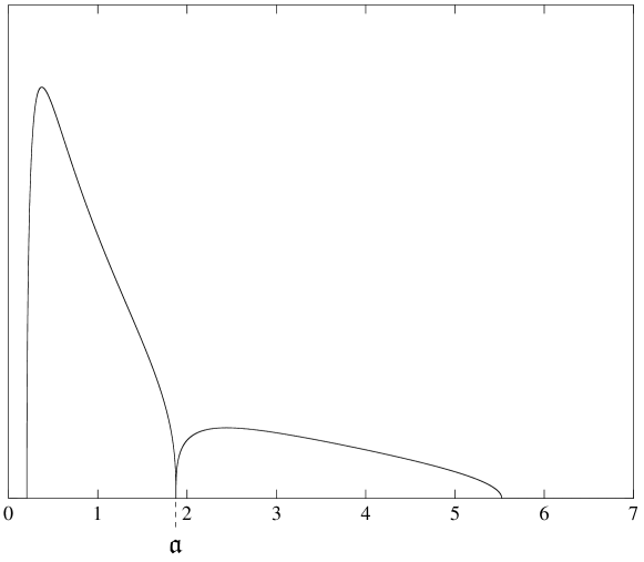
Figure 1: Plot of $\rho(x)$ with parameters $\gamma\simeq 0.336$ and $\nu=0.7\delta_{1}+0.3\delta_{3}$ with a cusp point $\mathfrak{a}$.

As stated in the introduction, we define a cusp point $\mathfrak{a}$ as an interior point where the density vanishes, namely $\mathfrak{a}\in\operatorname{int}(\operatorname{Supp}(\rho))$ such that $\rho(\mathfrak{a})=0$. In particular, $\mathfrak{c}=m(\mathfrak{a})\in\mathbb{R}$ by virtue of (2.9). Our first result states that the density $\rho(x)$ behaves like a cube root near a cusp point, provided that $\mathfrak{c}\in D$.

Proposition 1.

Let $\mathfrak{a}\in\operatorname{int}(\operatorname{Supp}(\rho))$ be such that $\rho(\mathfrak{a})=0$, and assume that $\mathfrak{c}=m(\mathfrak{a})\in D$. Then we have

$$g(\mathfrak{c})=\mathfrak{a}\,,\qquad g^{\prime}(\mathfrak{c})=g^{\prime\prime}(\mathfrak{c})=0\,,\qquad\textrm{and}\quad g^{(3)}(\mathfrak{c})>0\ .$$

Moreover,

$$\rho(x)=\frac{\sqrt{3}}{2\pi}\left(\frac{6}{g^{(3)}(\mathfrak{c})}\right)^{1/3}\big{|}x-\mathfrak{a}\big{|}^{1/3}(1+o(1))\ ,\qquad x\rightarrow\mathfrak{a}\,.$$ (2.14)

In particular, there exists $\eta>0$ such that for every $x\in(\mathfrak{a}-\eta,\mathfrak{a}+\eta)\setminus\{\mathfrak{a}\}$, we have $\rho(x)>0$.

Remark 2.1.

In the forthcoming local analysis for the random eigenvalues near a cusp point, we shall focus on cusp points $\mathfrak{a}$’s satisfying a regularity condition. This extra assumption automatically yields that $m(\mathfrak{a})\in D$, see Remark 2.5.

Conversely, we have the following result.

Proposition 2.

If $\mathfrak{c}\in D$ satisfies $g^{\prime}(\mathfrak{c})=g^{\prime\prime}(\mathfrak{c})=0$, then $\mathfrak{a}=g(\mathfrak{c})$ belongs to $\operatorname{int}(\operatorname{Supp}(\rho))$ and $\rho(\mathfrak{a})=0$. In particular, $g^{(3)}(\mathfrak{c})>0$ and $\rho(x)$ satisfies (2.14).

We prove Propositions 1 and 2 in sections 3.1 and 3.2 respectively. Their proofs are based on the fact that there is a strong relation between the property that $\mathfrak{a}=g(\mathfrak{c})$ is a cusp point and the local behaviour of $g$ near $\mathfrak{c}$. For an illustration of these propositions, we refer to Figure 2 where we displayed the graph of the map $g$ associated with the density from Figure 1.

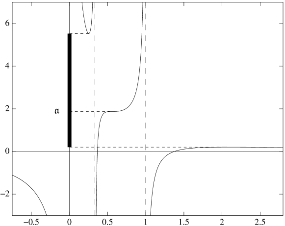
Figure 2: Plot of function $x\mapsto g(x)$ on $D$ for $\gamma\simeq 0.336$ and $\nu=0.7\delta_{1}+0.3\delta_{3}$. The vertical dotted lines are $g$’s asymptotes at $x=1/3$ and $x=1$. The thick segment on the vertical axis represents $\operatorname{Supp}(\rho)$ who is delimited by the local extrema of g (see Eq. (2.13)). The point $\mathfrak{a}$ is a cusp point.

We now turn to the hard edge setting.

2.4 Density behaviour near the hard edge

As usual in random matrix theory, the hard edge refers here to the origin when it belong to the limiting spectrum. In general, the limiting eigenvalue distribution may not display a hard edge, like in Figure 1. In fact, this is always the case when $\gamma\neq 1$, see [HHN-preprint, Proposition 2.4 (a),(c)]. Our next result states that there is a hard edge, namely $0\in\operatorname{Supp}(\rho)$, if and only if $\gamma=1$, and that in this case $\rho(x)$ blows up like an inverse square root at the origin. We furthermore relate the presence of a hard edge to the behaviour of $g$ near $\infty$. More precisely, since $\operatorname{Supp}(\nu)\subset(0,\infty)$ by Assumption 2, one can see from the definition (2.11) of $g$ that the map $g(1/z)$ is holomorphic at the origin. Thus, we have the analytic expansion as $z\to 0$

$$g(1/z)=g(\infty)+g^{\prime}(\infty)z+\frac{g^{\prime\prime}(\infty)}{2}z^{2}+\cdots$$ (2.15)

Clearly, $g(\infty)=0$ and the coefficients $g^{\prime}(\infty)$ and $g^{\prime\prime}(\infty)$ are respectively given by the first and second derivative of the map $z\mapsto g(1/z)$ evaluated at $z=0$.

Proposition 3.

The following three assertions are equivalent:

• $0\in\operatorname{Supp}(\rho)$

• $\gamma=1$

• $g^{\prime}(\infty)=0$

Moreover, we have $g^{\prime\prime}(\infty)=-2\gamma\int\lambda^{-1}\nu({\rm d}\lambda)<0$ and, if one of these assertions is satisfied, then

$$\rho(x)=\frac{1}{\pi}\left(\frac{2}{-g^{\prime\prime}(\infty)}\right)^{-1/2}x^{-1/2}\,(1+o(1))\ ,\qquad x\rightarrow 0_{+}\,.$$ (2.16)

Proposition 3 is proven in Section 3.3.

Remark 2.2.

There is an analogous statement for any left edge $\mathfrak{a}>0$ of the spectrum satisfying $\mathfrak{c}=m(\mathfrak{a})\in D$ which follows from [silverstein-choi-1995]; see also [HHN-esaim-preprint, Section 2] for further information. Indeed, in this case we have

$$g(\mathfrak{c})=\mathfrak{a},\qquad g^{\prime}(\mathfrak{c})=0,\qquad g^{\prime\prime}(\mathfrak{c})<0,$$

and furthermore, as $x\rightarrow\mathfrak{a}_{+}$,

$$\rho(x)=\frac{1}{\pi}\left(\frac{2}{-g^{\prime\prime}(\mathfrak{c})}\right)^{1/2}\big{(}x-\mathfrak{a}\big{)}^{1/2}(1+o(1))\ .$$

By analogy with this equation, the preimage $\mathfrak{c}\in D$ corresponding to the hard edge is $\mathfrak{c}=\infty$. The fact that it actually belongs to $D$ follows from Assumption 2(a).

Remark 2.3.

As we shall see in Section 3, proofs of Propositions 1, 2 and 3 only rely on the properties of the limiting eigenvalue distribution $\mu$, which do not depend on whether the entries of $\mathbf{X}_{N}$ are Gaussian or not. More precisely, the exact assumptions required for these propositions are that the entries of $\mathbf{X}_{N}$ are i.i.d centered random variables with variance one, Assumption 2–(b), and that $\mu(\{0\})=0$ (which follows from Assumption 2–(a)), see [mar-and-pas-67, silverstein-choi-1995].

2.5 The Pearcey kernel and fluctuations near a cusp point

Our next result essentially states that the random eigenvalues of $\mathbf{M}_{N}$, properly scaled near a regular cusp point, asymptotically behave like the determinantal point process associated with the Pearcey kernel, provided that an extra condition on a speed parameter is satisfied.

In order to state this result, we first introduce this limiting point process. Next, we define what we mean by regular, and provide the existence of appropriate scaling parameters. After that, we finally state our result for the fluctuations near a cusp point.

2.5.1 Determinantal point processes

A point process on $\mathbb{R}$ (or in a subset therein), namely a probability distribution $\mathbb{P}$ over the locally finite discrete subsets $(y_{i})$ of $\mathbb{R}$, is determinantal if there exists an appropriate kernel ${\rm K}(x,y):\mathbb{R}\times\mathbb{R}\to\mathbb{R}$ which characterizes the correlation functions in the following way: For every $k\geqslant 1$ and every compactly supported Borel function $\Phi:\mathbb{R}^{k}\to\mathbb{R}$, we have

$$\mathbb{E}\left[\sum_{y_{i_{1}}\neq\,\cdots\,\neq\,y_{i_{k}}}\Phi(y_{i_{1}},\ldots,y_{i_{k}})\right]=\int_{\mathbb{R}}\cdots\int_{\mathbb{R}}\Phi(y_{1},\ldots,y_{k})\det\Big{[}{\rm K}(y_{i},y_{j})\Big{]}_{i,j=1}^{k}{\rm d}y_{1}\cdots{\rm d}y_{k}\,.$$ (2.17)

In particular, the gap probabilities can be expressed as Fredholm determinants. Namely, given any interval $J\subset\mathbb{R}$, the probability that the point process avoids $J$ reads

$$\mathbb{P}\Big{(}(y_{i})\cap J=\varnothing\Big{)}=1+\sum_{k=1}^{\infty}\frac{(-1)^{k}}{k!}\int_{J}\cdots\int_{J}\det\Big{[}{\rm K}(y_{i},y_{j})\Big{]}_{i,j=1}^{k}{\rm d}y_{1}\cdots{\rm d}y_{k}\,,$$ (2.18)

and the right hand side is the Fredholm determinant $\det(I-{\rm K})_{L^{2}(J)}$ of the integral operator acting on $L^{2}(J)$ with kernel ${\rm K}(x,y)$, provided that it makes sense. For instance, if one assumes that $J$ is a compact interval, which is enough for the purpose of this work, then $\det(I-{\rm K})_{L^{2}(J)}$ is well-defined and finite as soon as ${\|{\rm K}\|}_{J}=\sup_{x,y\in J}|{\rm K}(x,y)|<\infty$. Moreover, the map ${\rm K}(x,y)\mapsto\det(I-{\rm K})_{L^{2}(J)}$ is Lipschitz with respect to ${\|\cdot\|}_{J}$ when restricted to the kernels satisfying ${\|{\rm K}\|}_{J}<\infty$ (see e.g. [3, Lemma 3.4.5]). We refer the reader to [Hu, JoR, 3] for further information on determinantal point processes.

2.5.2 The Pearcey kernel

Given any $\tau\in\mathbb{R}$, consider the Pearcey-like integral functions

$$\phi(x)=\frac{1}{2i\pi}\int_{\Sigma}e^{xz-\tau\frac{z^{2}}{2}+\frac{z^{4}}{4}}{\rm d}z,\qquad\psi(y)=\frac{1}{2i\pi}\int_{-i\infty}^{i\infty}e^{-yw+\tau\frac{w^{2}}{2}-\frac{w^{4}}{4}}{\rm d}w,$$

where the contour $\Sigma$ has two non-intersecting components, one which goes from $e^{i\pi/4}\infty$ to $e^{-i\pi/4}\infty$, whereas the other one goes from $e^{-3i\pi/4}\infty$ to $e^{3i\pi/4}\infty$. More precisely, we parametrize here this contour by

$$\Sigma=\left\{\pm e^{i\theta}:\;\theta\in[-\pi/4,\pi/4]\right\}\,\cup\,\left\{te^{\pm i\pi/4}:\;t\in(-\infty,-1]\cup[1,+\infty)\right\}\,,$$ (2.19)

with the orientation as shown in Figure 3.

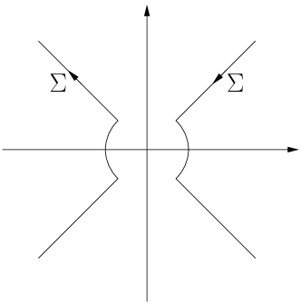
Figure 3: The contour $\Sigma$.

It follows from their definitions that the functions $\phi$ and $\psi$ satisfy the respective differential equations

$$\phi^{\prime\prime\prime}(x)-\tau\phi^{\prime}(x)+x\phi(x)=0\,,\qquad\psi^{\prime\prime\prime}(y)-\tau\psi^{\prime}(y)-y\psi(y)=0\,.$$

The Pearcey kernel is then defined for $x,y\in\mathbb{R}$ by

$${\rm K}_{\rm Pe}^{(\tau)}(x,y)=\frac{\phi^{\prime\prime}(x)\psi(y)-\phi^{\prime}(x)\psi^{\prime}(y)+\phi(x)\psi^{\prime\prime}(y)-\tau\phi(x)\psi(y)}{x-y}\ ,$$ (2.20)

see for instance [9]. One can alternatively represent this kernel as a double contour integral

$${\rm K}_{{\rm Pe}}^{(\tau)}(x,y)=\frac{1}{(2i\pi)^{2}}\int_{\Sigma}{\rm d}z\int_{-i\infty}^{\,i\infty}{\rm d}w\,\frac{1}{w-z}e^{xz-\frac{\tau z^{2}}{2}+\frac{z^{4}}{4}-yw+\frac{\tau w^{2}}{2}-\frac{w^{4}}{4}}\ ,$$ (2.21)

from which one can easily see the symmetry ${\rm K}_{{\rm Pe}}^{(\tau)}(x,y)={\rm K}_{{\rm Pe}}^{(\tau)}(-x,-y)$ by performing the changes of variables $z\mapsto-z$ and $w\mapsto-w$.

The Pearcey kernel first appeared in the works of Brézin and Hikami [8, 9] when studying the eigenvalues of a specific additive perturbation of a GUE random matrix near a cusp point. Subsequent generalizations have been considered by Tracy and Widom [tracy-widom-pearcey], and a Riemann-Hilbert analysis has been performed by Bleher and Kuijlaars [6] as well. This kernel also arises in the description of random combinatorial models, such as certain plane partitions [OR07]. Furthermore, it has been established that the gap probabilities for the associated point process satisfy differential equations. For instance, $\log\det(I-{\rm K}^{(\tau)}_{\rm Pe})_{L^{2}(s,t)}$ satisfies PDEs with respect to the variables $s$, $t$ and $\tau$, see [tracy-widom-pearcey, 5, 2], which should be compared to the connection between the Tracy-Widom distribution and the Painlevé II equation.

2.5.3 The regularity condition

We start with the following definition.

Definition 2.4.

A cusp point $\mathfrak{a}$ is regular if $\mathfrak{c}=m(\mathfrak{a})$ satisfies

$$\liminf_{N\to\infty}\min_{j=1}^{n}\left|\mathfrak{c}-\frac{1}{\lambda_{j}}\right|>0.$$ (2.22)

The regularity condition (2.22) has been considered in [HHN-preprint] when dealing with soft edges, to ensure the appearance of the Tracy-Widom distribution. Similarly here, as we soon shall see, this condition enables the Pearcey kernel to arise at a cusp point. Moreover, the behaviour of $\rho(x)$ at such cusp points is well described by Proposition 1, as explained in the next remark.

Remark 2.5.

If $\mathfrak{a}$ is a regular cusp point, then it follows from the weak convergence $\nu_{N}\to\nu$ and the definition of $D$ that necessarily $\mathfrak{c}=m(\mathfrak{a})\in D$. Thus, $\mathfrak{a}$ satisfies the hypothesis of Proposition 1. In particular, we have $\mathfrak{a}=g(\mathfrak{c})$ and $\rho(x)$ behaves like a cube root near $\mathfrak{a}$.

Finally, the regularity assumption yields the existence of natural scaling parameters for the eigenvalue local asymptotics. Consider the counterpart of the map $g$ introduced in (2.11) after replacing $\nu$ by $\nu_{N}$, see (2.3), and $\gamma$ by $n/N$, namely

$$g_{N}(z)=\frac{1}{z}+\frac{n}{N}\int\frac{\lambda}{1-z\lambda}\,\nu_{N}({\rm d}\lambda)\,.$$ (2.23)

The map $g_{N}$ is the inverse Cauchy transform of a probability measure $\mu_{N}$ usually referred to as deterministic equivalent for the random eigenvalues distribution of $\mathbf{M}_{N}$, see [HHN-esaim-preprint, Section 3.2]. According to Section 2.2, $\mu_{N}$ has a decomposition of the form (2.10). In particular, it has a density $\rho_{N}$ on $(0,+\infty)$ which is analytic wherever it is positive.

The next proposition provides an appropriate sequence of finite–$N$ approximations of $\mathfrak{c}$, which we will use in the definition of the scaling parameters.

Proposition 4.

Let $\mathfrak{a}=g(\mathfrak{c})$ be a regular cusp point. Then there exists a sequence $(\mathfrak{c}_{N})$ of real numbers, unique up to a finite number of terms, converging to $\mathfrak{c}$ and such that for every $N$ large enough, we have $\mathfrak{c}_{N}\in D$ and

$$\lim_{N\to\infty}g_{N}(\mathfrak{c}_{N})=g(\mathfrak{c})\ ,\qquad\lim_{N\to\infty}g_{N}^{\prime}(\mathfrak{c}_{N})=0\ ,\qquad g_{N}^{\prime\prime}(\mathfrak{c}_{N})=0\qquad\textrm{and}\qquad g_{N}^{(3)}(\mathfrak{c}_{N})>0\ .$$

This proposition is the counterpart of [HHN-preprint, Proposition 2.7], with a similar proof. Let us only provide a sketch here: Combined with Montel’s theorem, the regularity condition ensures that $g_{N}^{(k)}$ converge uniformly to $g^{(k)}$ on a neighbourhood of $\mathfrak{c}$ for every $k\geqslant 0$. The proposition then follows by applying Hurwitz’s theorem to $g^{\prime\prime}_{N}$ since $\mathfrak{c}$ is a simple root for $g^{\prime\prime}$, according to Proposition 2.14.

Let us emphasize that there is however an important difference with regular soft edges as described in [HHN-preprint], where it was shown that if $\mathfrak{a}=g(\mathfrak{c})$ is a regular soft edge for $\mu$, then $g_{N}(\mathfrak{c}_{N})$ is a soft edge for $\mu_{N}$.

Remark 2.6.

A regular cusp point may not be the limit of finite–$N$ cusp points. More precisely, if $\mathfrak{a}=g(\mathfrak{c})$ is a regular cusp point, then in particular $g^{\prime}(\mathfrak{c})=g^{\prime\prime}(\mathfrak{c})=0$. However, this only ensures the existence of a sequence $(\mathfrak{c}_{N})$ such that $g_{N}^{\prime\prime}(\mathfrak{c}_{N})=0$. A priori, $g_{N}^{\prime}(\mathfrak{c}_{N})$ converges to zero as $N\to\infty$ but might not be equal to zero. In fact, it is not hard to show we have the following alternatives:

• if $g_{N}^{\prime}(\mathfrak{c}_{N})=0$, then $g_{N}(\mathfrak{c}_{N})$ is a cusp point for $\mu_{N}$;

• if $g^{\prime}_{N}(\mathfrak{c}_{N})>0$, then the density $\rho_{N}$ is positive in a vicinity of $g_{N}(\mathfrak{c}_{N})$;

• if $g^{\prime}_{N}(\mathfrak{c}_{N})<0$, then $g_{N}(\mathfrak{c}_{N})$ does not belong to the support of $\mu_{N}$.

We are finally in position to state our result concerning the eigenvalue behaviour at a regular cusp point.

2.5.4 Fluctuations around a cusp point

Thanks to Assumption 1, the random eigenvalues $(x_{i})$ of $\mathbf{M}_{N}$ form a determinantal point process with respect to a kernel ${\rm K}_{N}(x,y)$, see [4, On]. An explicit formula for this kernel is provided in Section 4. The main result of this section is the local uniform convergence of this kernel, properly scaled, towards the Pearcey kernel.

Theorem 5.

Let $\mathfrak{a}=g(\mathfrak{c})$ be a regular cusp point. Let $(\mathfrak{c}_{N})$ be the sequence associated to $\mathfrak{c}$ coming from Proposition 4. Assume moreover that the following decay assumption holds true: There exists $\kappa\in\mathbb{R}$ such that

$$\sqrt{N}g^{\prime}_{N}(\mathfrak{c}_{N})\xrightarrow[N\to\infty]{}\kappa\ .$$ (2.24)

Set

$$\mathfrak{a}_{N}=g_{N}(\mathfrak{c}_{N})\ ,\qquad\sigma_{N}=\left(\frac{6}{g^{(3)}_{N}(\mathfrak{c}_{N})}\right)^{1/4}\ ,\qquad\tau=-\kappa\left(\frac{6}{g^{(3)}(\mathfrak{c})}\right)^{1/2},$$ (2.25)

so that $\mathfrak{a}_{N}\to\mathfrak{a}$ and $\mathfrak{\sigma}_{N}\to(6/g^{(3)}(\mathfrak{c}))^{1/4}>0$ as $N\to\infty$ by Proposition 4. Then, we have

$$\frac{1}{N^{3/4}\sigma_{N}}\,{\rm K}_{N}\left(\mathfrak{a}_{N}+\frac{x}{N^{3/4}\sigma_{N}},\mathfrak{a}_{N}+\frac{y}{N^{3/4}\sigma_{N}}\right)\xrightarrow[N\to\infty]{}{\rm K}_{\rm Pe}^{(\tau)}(x,y)$$ (2.26)

uniformly for $x,y$ in compact subsets of $\mathbb{R}$.

This result was obtained by Mo [Mo2] in the special case where the matrix $\mathbf{\Sigma}_{N}$ has exactly two distinct eigenvalues (each with multiplicities proportional $N$), by means of a Riemann-Hilbert asymptotic analysis.

Notice that if $(x_{i})$ is determinantal with kernel ${\rm K}_{N}(x,y)$, then $(N^{3/4}\sigma_{N}(x_{i}-\mathfrak{a}_{N}))$ is determinantal with the kernel given by the left hand side of (2.26). Thus, having in mind Section 2.5.1, a direct consequence of this theorem is the convergence of the compact gap probabilities.

Corollary 2.7.

Under the assumptions of Theorem 5, we have for every $s,t\in\mathbb{R}$,

$$\mathbb{P}\left(\left(N^{3/4}\sigma_{N}(x_{i}-\mathfrak{a}_{N})\right)\cap[s,t]=\varnothing\right)\xrightarrow[N\to\infty]{}\det(I-{\rm K}^{(\tau)}_{\rm Pe})_{L^{2}(s,t)}\ .$$ (2.27)

We now make a few comments on the assumption (2.24).

Remark 2.8.

The decay assumption (2.24) roughly states that the cusp point $\mathfrak{a}=g(\mathfrak{c})$ appears fast enough. More precisely, for a cusp point $\mathfrak{a}=g(\mathfrak{c})$, one has in particular $g^{\prime}(\mathfrak{c})=0$.

• If $\kappa>0$, then $g^{\prime}_{N}(\mathfrak{c}_{N})>0$ for large $N$. According to Remark 2.6, the density $\rho_{N}$ is positive near $g_{N}(\mathfrak{c}_{N})$ and will converge to zero to asymptotically give birth to a cusp point. The family of densities $\rho_{N}$ display a sharp non-negative minimum at $g_{N}(\mathfrak{c}_{N})$ converging to zero which may be thought of as the erosion of a valley, see the thin curve in Figure 4.

• If $\kappa<0$, then $g^{\prime}_{N}(\mathfrak{c}_{N})<0$ for large $N$ and the density $\rho_{N}$ vanishes in a vicinity of $g_{N}(\mathfrak{c}_{N})$. However, this interval will shrink and asymptotically disappear. Thus, two connected components of the support of $\mu_{N}$ move towards one another (moving cliffs), see the dotted curve in Figure 4.

The assumption (2.24) is an indication on the speed at which the bottom of the valley reaches zero $(\kappa>0)$, or at which the two cliffs approach one another $(\kappa<0)$. See [HHN-esaim-preprint] for a more in-depth discussion.

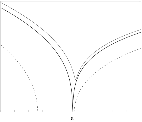
Figure 4: Zoom of the density of $\mu_{N}$ near the cusp point $\mathfrak{a}$. The thick curve is the density of $\mu$ in the framework of Figure 1. The thin curve (resp. the dotted curve) is the density of $\mu_{N}$ when $\sqrt{N}g^{\prime}_{N}(\mathfrak{c}_{N})>0$ (resp. $\sqrt{N}g^{\prime}_{N}(\mathfrak{c}_{N})<0$).

Remark 2.9.

When the assumption (2.24) is not satisfied, namely when $g^{\prime}_{N}(\mathfrak{c}_{N})$ goes to zero as $N\to\infty$ (which is always true by Proposition 4) slow enough so that $\sqrt{N}g^{\prime}_{N}(\mathfrak{c}_{N})$ diverges to plus or minus infinity, we do not expect the Pearcey kernel to arise. See [HHN-esaim-preprint] for further discussion.

The proof of Theorem 5 is provided in Section 4.

2.6 Asymptotic expansion at the hard edge

Our last result concerns the behaviour of the smallest random eigenvalue of $\mathbf{M}_{N}$ when the hard edge is present. Recall that $n/N\to\gamma$. By Proposition 3, the limiting density displays a hard edge if and only if $\gamma=1$. With this respect, we restrict ourselves here to the case $n=N+\alpha$ where $\alpha\in\mathbb{Z}$ is fixed and does not depend on $N$.

2.6.1 The Bessel kernel

The Bessel function of the first kind $J_{\alpha}$ with parameter $\alpha\in\mathbb{Z}$ is defined by

$$J_{\alpha}(x)=\left(\frac{x}{2}\right)^{\alpha}\sum_{n=0}^{\infty}\frac{(-1)^{n}}{n!\,\Gamma(n+\alpha+1)}\left(\frac{x}{2}\right)^{2n},\qquad x>0\ ,$$ (2.28)

with the convention that, when $\alpha<0$, the first $|\alpha|$ terms in the series vanish (since the Gamma function $\Gamma$ has simple poles on the non-positive integers).

The Bessel kernel is then defined for $x,y>0$ by

$${\rm K}_{{\rm Be}}^{(\alpha)}(x,y)=\frac{\sqrt{y}J_{\alpha}(\sqrt{x})J_{\alpha}^{\prime}(\sqrt{y})-\sqrt{x}J_{\alpha}^{\prime}(\sqrt{x})J_{\alpha}(\sqrt{y})}{2(x-y)}\ .$$ (2.29)

One can alternatively express it as a double contour integral,

$${\rm K}_{{\rm Be}}^{(\alpha)}(x,y)=\frac{1}{(2i\pi)^{2}}\left(\frac{y}{x}\right)^{\frac{\alpha}{2}}\oint_{|z|=r}\frac{{\rm d}z}{z}\oint_{|w|=R}\frac{{\rm d}w}{w}\frac{1}{z-w}\left(\frac{z}{w}\right)^{\alpha}e^{-\frac{x}{z}+\frac{z}{4}+\frac{y}{w}-\frac{w}{4}}\ ,$$ (2.30)

where $0<r<R$ and the contours are simple and oriented counterclockwise, see for instance [HHN-preprint, Lemma 6.2]. We set for convenience

$$F_{\alpha}(s)=\det\big{(}I-{\rm K}_{{\rm Be}}^{(\alpha)}\big{)}_{L^{2}(0,s)},\qquad s>0,$$ (2.31)

where the right hand side stands for the Fredholm determinant of the restriction to $L^{2}(0,s)$ of the integral operator ${\rm K}_{{\rm Be}}^{(\alpha)}$. According to (2.18), $F_{\alpha}(s)$ is the probability that the smallest particle of the determinantal point process associated with the Bessel kernel is larger than $s$. Tracy and Widom [tracy-widom-bessel-94] established that certain simple transformations of $\log F_{\alpha}(s)$ satisfy Painlevé equations (Painlevé III and Painlevé V are involved).

2.6.2 Correction for the smallest eigenvalue’s fluctuations

We denote by $x_{\min}$ the smallest random eigenvalue of $\mathbf{M}_{N}$, namely

$$x_{\min}=\begin{cases}x_{1}&\mbox{ if }\alpha\geqslant 0,\\ x_{1-\alpha}&\mbox{ if }\alpha<0.\end{cases}$$ (2.32)

Our last result is stated as follows.

Theorem 6.

Assume $n=N+\alpha$ where $\alpha\in\mathbb{Z}$ is fixed and does not depend on $N$. Set

$$\sigma_{N}=\frac{4}{N}\sum_{j={1}}^{n}\frac{1}{\lambda_{j}}\qquad\textrm{and}\qquad\zeta_{N}=\frac{8}{N}\sum_{i=1}^{N}\frac{1}{\lambda_{i}^{2}}\ ,$$ (2.33)

so that

$$\sigma_{N}\xrightarrow[N\to\infty]{}4\int\frac{\nu({\rm d}\lambda)}{\lambda}\ >\ 0\qquad\textrm{and}\qquad\zeta_{N}\xrightarrow[N\to\infty]{}8\int\frac{\nu({\rm d}\lambda)}{\lambda^{2}}\ >\ 0$$

by Assumption 2. Then, for every $s>0$, we have as $N\to\infty$,

$$\mathbb{P}\Big{(}N^{2}\sigma_{N}\,x_{\min}\geqslant s\Big{)}=F_{\alpha}(s)-\frac{1}{N}\left(\frac{\alpha\zeta_{N}}{\sigma_{N}^{2}}\right)s\frac{{\rm d}}{{\rm d}s}F_{\alpha}(s)+{\mathcal{O}}\left({\frac{1}{N^{2}}}\right)\ .$$ (2.34)

The convergence towards $F_{\alpha}(s)$ has been first observed by Forrester [16] when $\mathbf{\Sigma}_{N}$ is the identity. As for the general $\mathbf{\Sigma}_{N}$ case, it has been established by the authors in [HHN-preprint]. An explicit formula for the $1/N$-correction term was conjectured when $\mathbf{\Sigma}_{N}$ is the identity by Edelman, Guionnet and Péché [13], a conjecture proved true soon after by Perret and Schehr [PS] and Bornemann [7], with different techniques. We thus generalize this formula to the general $\mathbf{\Sigma}_{N}$ case. The strategy of the proof is rather similar to Bornemann’s one: It relies on an identity involving the resolvent of ${\rm K}_{\rm Be}^{(\alpha)}$ obtained by Tracy and Widom, although we cannot rely on existing estimates for the kernel in this general setting.

Remark 2.10.

In fact, as we shall see in the proof of Theorem 6 (see Remark 5.2), our method easily yields for every $s>0$ an expansion of the form

$$\mathbb{P}\Big{(}N^{2}\sigma_{N}\,x_{\min}\geqslant s\Big{)}=F_{\alpha}(s)+\sum_{\ell=1}^{L}\frac{1}{N^{\ell}}C_{N,\ell}^{(\alpha)}(s)+{\mathcal{O}}\left({\frac{1}{N^{L+1}}}\right)$$ (2.35)

for every $L\geqslant 1$ as $N\to\infty$. Although we are able to provide a close formula for the coefficient $C_{N,1}^{(\alpha)}(s)$ (as stated in Theorem 6) thanks to a formula due to Tracy and Widom, to the best of our knowledge the next order coefficients do not seem to benefit from such a simple representation.

We prove Theorem 6 in Section 5.

3 Proofs of the limiting density behaviours

This section is devoted to the proofs of Proposition 1, 2 and 3.

We first recall a few facts stated in Section 2.2 that we shall use in the forthcoming proofs: The map $m$ is the Cauchy-Stieltjes transform (2.7); it is analytic on $\mathbb{C}_{+}$ and extends continuously to $\mathbb{C}_{+}\cup\mathbb{R}^{*}$. Moreover, $\mathfrak{Im}(m(x))=-\pi\rho(x)$ for every $x\in\mathbb{R}^{*}$. The map $g$ defined in (2.11) is analytic on $\mathbb{C}_{+}\cup\mathbb{C}_{-}\cup D$. In particular, $g^{\prime}$ has isolated zeroes on $D$. Moreover, after noticing that $m(\mathbb{C}_{+})\subset\mathbb{C}_{-}$, we have the identity $g(m(z))=z$ for every $z\in\mathbb{C}_{+}$.

We start with a simple but useful fact, which follows by taking the limit $z\in\mathbb{C}_{+}\to x$ in the previous identity and using the continuity of $m$ and $g$ on their respective domains:

Lemma 3.1.

If $x\in\mathbb{C}_{+}\cup\mathbb{R}^{*}$ is such that $m(x)\in\mathbb{C}_{-}\cup D$, then $g(m(x))=x$.

We will also use the following property.

Lemma 3.2.

If $\mathfrak{a}\in\operatorname{Supp}(\rho)$ satisfies $\rho(\mathfrak{a})=0$ and $\mathfrak{c}=m(\mathfrak{a})\in D$, then $g^{\prime}(\mathfrak{c})=0$.

Proof.

Consider the map

$$G(m)=-\frac{1}{|m|^{2}}+\gamma\int\frac{\lambda^{2}}{|1-\lambda m|^{2}}\nu({\rm d}\lambda)\ ,\qquad m\in\mathbb{C}_{-}\cup D,$$ (3.1)

and notice it is continuous on its definition domain by dominated convergence. It follows from the definition (2.11) of $g$ that $G(m)=g^{\prime}(m)$ when $m\in D$, and moreover that for every $m\in\mathbb{C}_{-}$ we have the identity

$$\mathfrak{Im}(g(m))=\mathfrak{Im}(m)G(m).$$

By using the fact that $g(m(z))=z$ on $\mathbb{C}_{+}$, we thus obtain for every $z\in\mathbb{C}_{+}$,

$$\mathfrak{Im}(z)=\mathfrak{Im}(m(z))G(m(z)).$$ (3.2)

If $x\in\mathbb{R}^{*}$ is such that $\rho(x)>0$, then by letting $z\in\mathbb{C}_{+}\to x$ in (3.2) we see that necessarily $G(m(x))=0$ because $\lim_{z\to x}\mathfrak{Im}(m(z))=\mathfrak{Im}(m(x))=-\pi\rho(x)<0$. Now, since $\mathfrak{a}\in\operatorname{Supp}(\rho)$ by assumption, there exists a sequence $(x_{k})$ such that $x_{k}\to\mathfrak{a}$ as $k\to\infty$ and $\rho(x_{k})>0$, and hence $G(m(x_{k}))=0$. Since $m(x_{k})\to m(\mathfrak{a})=\mathfrak{c}$ and $\mathfrak{c}\in D$, this yields $g^{\prime}(\mathfrak{c})=G(\mathfrak{c})=0$. ∎

3.1 Density behaviour near a cusp point: Proof of Proposition 1

We now turn to the proof of the first proposition.

Proof.

Assume that $\mathfrak{a}\in\operatorname{int}(\operatorname{Supp}(\rho))$ and $\rho(\mathfrak{a})=0$. Set $\mathfrak{c}=m(\mathfrak{a})$ and assume moreover that $\mathfrak{c}\in D$. Thus, the facts that $g(\mathfrak{c})=\mathfrak{a}$ and $g^{\prime}(\mathfrak{c})=0$ directly follows from Lemma 3.1 and Lemma 3.2.

First, we prove that $g^{\prime\prime}(\mathfrak{c})=0$. To do so, we show that $g^{\prime}>0$ on $(\mathfrak{c}-\eta,\mathfrak{c}+\eta)-\{\mathfrak{c}\}$ for some $\eta>0$. Since $g^{\prime}(\mathfrak{c})=0$ this would indeed yield that $\mathfrak{c}$ is a local extremum for $g^{\prime}$. We proceed by contradiction: Assume there exists a sequence $(x_{k})$ in $D-\{\mathfrak{c}\}$ such that $x_{k}\to\mathfrak{c}$ and $g^{\prime}(x_{k})\leqslant 0$. Since $g^{\prime}$ has isolated zeroes on $D$, necessarily $g^{\prime}(x_{k})<0$ for every $k$ large enough. It then follows from (2.13) that $g(x_{k})\in\mathbb{R}-\operatorname{Supp}(\rho)$ and, since $g(x_{k})\to g(\mathfrak{c})=\mathfrak{a}$, this contradicts the assumption that $\mathfrak{a}\in\operatorname{int}(\operatorname{Supp}(\rho))$.

Next, we similarly show that there exists $\eta>0$ such that

$$x\in(\mathfrak{a}-\eta,\mathfrak{a}+\eta)-\{\mathfrak{a}\}\quad\Rightarrow\quad\rho(x)>0\ .$$ (3.3)

We will use (3.3) later on in this proof. Assume there exists a sequence $(x_{k})$ in $\mathbb{R}^{*}-\{\mathfrak{a}\}$ such that $x_{k}\to\mathfrak{a}$ and $\rho(x_{k})=0$. Since $\mathfrak{a}\in\operatorname{int}(\operatorname{Supp}(\rho))$ and $m(\mathfrak{a})\in D$ by assumption, then $x_{k}\in\operatorname{Supp}(\rho)$ and $m(x_{k})\in D$ for every $k$ large enough. Moreover, we have $m(x_{k})\to m(\mathfrak{a})$, but since Lemma 3.2 then yields $g^{\prime}(m(x_{k}))=0$, this contradicts that $g^{\prime}$ has isolated zeroes on $D$ and (3.3) follows.

Now, we show that $g^{(3)}(\mathfrak{c})>0$ by direct computation. Recalling the definition (2.11) of $g$, the equation $g^{\prime\prime}(\mathfrak{c})=0$ reads

$$-\frac{1}{\mathfrak{c}^{3}}=\gamma\int\frac{\lambda^{3}}{(1-\lambda\mathfrak{c})^{3}}\,\nu({\rm d}\lambda)\ .$$

As a consequence, we obtain

$$\frac{1}{6}g^{(3)}(\mathfrak{c}) =-\frac{1}{{\mathfrak{c}}^{4}}+\gamma\int\frac{\lambda^{4}}{(1-\lambda{\mathfrak{c}})^{4}}\,\nu({\rm d}\lambda)$$

$$=\frac{1}{{\mathfrak{c}}}\left(\gamma\int\frac{\lambda^{3}}{(1-\lambda\mathfrak{c})^{3}}\,\nu({\rm d}\lambda)\right)+\gamma\int\frac{\lambda^{4}}{(1-{\lambda\mathfrak{c}})^{4}}\,\nu({\rm d}\lambda)$$

$$=\gamma\int\frac{\lambda^{3}}{\mathfrak{c}(1-\lambda\mathfrak{c})^{4}}\,\nu({\rm d}\lambda)>0\ .$$

We finally turn to the proof of the cube root behaviour (2.14). Since $g^{\prime}(\mathfrak{c})=g^{\prime\prime}(\mathfrak{c})=0$ and $g^{(3)}(\mathfrak{c})>0$, there exists an analytic map $\varphi$ defined on a complex neighbourhood of $\mathfrak{c}$ such that $g(m)-\mathfrak{a}=\varphi(m)^{3}$ and $\varphi^{\prime}(\mathfrak{c})\neq 0$, see e.g. [book-rudin-real-complex, Theorem 10.32]. In particular, we have $\varphi^{\prime}(\mathfrak{c})^{3}=g^{(3)}(\mathfrak{c})/6\stackrel{{\scriptstyle\triangle}}{{=}}C>0$. Moreover, the inverse function theorem yields that $\varphi$ has a local inverse $\varphi^{-1}$, defined on a neighbourhood of zero, such that $\varphi^{-1}(0)=\mathfrak{c}$ and $\left(\varphi^{-1}\right)^{{}^{\prime}}(0)=1/\varphi^{\prime}(\mathfrak{c})$. If $|x-\mathfrak{a}|$ is small enough, then $\rho(x)>0$ by (3.3), hence $m(x)\in\mathbb{C}_{-}$, and we have $g(m(x))=x$ by Lemma 3.1. In particular, we have

$$\varphi(m(x))^{3}=g(m(x))-\mathfrak{a}=x-\mathfrak{a}$$

and, by taking the cube root (principal determination), applying $\varphi^{-1}$, and performing a Taylor expansion, we obtain

$$m(x)=\mathfrak{c}+\boldsymbol{j}\left(\frac{x-\mathfrak{a}}{C}\right)^{1/3}+o(x-\mathfrak{a})^{1/3}$$ (3.4)

where $\boldsymbol{j}$ is an undetermined cube root of unity. Since $m(x)\in\mathbb{C}_{-}$, necessarily $\boldsymbol{j}=\exp(2i\pi/3)$ if $x<\mathfrak{a}$ and $\boldsymbol{j}=\exp(-2i\pi/3)$ if $x>\mathfrak{a}$. Finally, (2.14) follows by taking the imaginary part in (3.4).

Proof of Proposition 1 is therefore complete.

∎

3.2 Identification of a cusp point: Proof of Proposition 2

The main part of the proof consists in showing the following lemma.

Lemma 3.3.

Let $\mathfrak{c}\in D$ such that $g^{\prime}(\mathfrak{c})=0$. Then $g(\mathfrak{c})\neq 0$ and $m(g(\mathfrak{c}))=\mathfrak{c}$.

Equipped with Lemma 3.3, let us first show how the proposition follows.

Proof of Proposition 2.

Assume that $\mathfrak{c}\in D$ satisfies $g^{\prime}(\mathfrak{c})=g^{\prime\prime}(\mathfrak{c})=0$ and set $\mathfrak{a}=g(\mathfrak{c})$. In particular, $\mathfrak{a}\in\operatorname{Supp}(\rho)$ by (2.13), and we just have to show that $\rho(\mathfrak{a})=0$ and $\mathfrak{a}\notin\partial\operatorname{Supp}(\rho)$. We know from Lemma 3.3 that $\mathfrak{a}\neq 0$ and $m(\mathfrak{a})=\mathfrak{c}$. As a consequence, $\rho(\mathfrak{a})=-\mathfrak{Im}(m(\mathfrak{a}))/\pi=0$. Finally, since $\mathfrak{a}=g(\mathfrak{c})$ with $\mathfrak{c}\in D$ and $\rho(\mathfrak{a})=0$, then [silverstein-choi-1995, Theorem 5.2] shows the condition $\mathfrak{a}\in\partial\operatorname{Supp}(\rho)$ requires $g^{\prime\prime}(\mathfrak{c})\neq 0$, which is not possible by assumption.

∎

We now prove the lemma.

Proof of Lemma 3.3.

For every $m\in D$ we have

$$g(m)+mg^{\prime}(m)=\gamma\int\frac{\lambda}{(1-\lambda m)^{2}}\,\nu({\rm d}\lambda)\neq 0\ ,$$

and because $g^{\prime}(\mathfrak{c})=0$ by assumption, by taking $m=\mathfrak{c}$ we see that necessarily $g(\mathfrak{c})\neq 0$. Let us now prove that $m(g(\mathfrak{c}))=\mathfrak{c}$. Introduce for convenience the map

$$\Phi(z)=\frac{z}{1-z}\ .$$

By combining the fixed point equation (2.8) for $m(z)$ with $z\in\mathbb{C}_{+}$ and that

$$\frac{1}{\mathfrak{c}}=g(\mathfrak{c})-g(\mathfrak{c})+\frac{1}{\mathfrak{c}}=g(\mathfrak{c})-\gamma\int\frac{\lambda}{1-\mathfrak{c}\lambda}\,\nu({\rm d}\lambda)\ ,$$

we obtain

$$m(z)-\mathfrak{c} =\mathfrak{c}m(z)\left(\frac{1}{\mathfrak{c}}-\frac{1}{m(z)}\right)$$

$$=\mathfrak{c}m(z)(g(\mathfrak{c})-z)+\gamma(m(z)-\mathfrak{c})\int\Phi(\lambda m(z))\Phi(\lambda\mathfrak{c})\,\nu({\rm d}\lambda)\ .$$

By reorganizing this equation as

$$(m(z)-\mathfrak{c})\Bigl{(}1-\gamma\int\Phi(\lambda m(z))\,\Phi(\lambda\mathfrak{c})\,\nu({\rm d}\lambda)\Bigr{)}=(g(\mathfrak{c})-z)m(z)\mathfrak{c}\ ,$$ (3.5)

we see the lemma would follow by taking the limit $z\in\mathbb{C}_{+}\to g(\mathfrak{c})\in\mathbb{R}^{*}$ assuming that

$$\left|1-\gamma\int\Phi(\lambda m(z))\,\Phi(\lambda\mathfrak{c})\,\nu({\rm d}\lambda)\right|\geqslant C|m(z)-\mathfrak{c}|^{2}\ ,\qquad z\in\mathbb{C}_{+}\to g(\mathfrak{c}),$$ (3.6)

for some constant $C>0$. To show (3.6), we start by writing

$$\left|1-\gamma\int\Phi(\lambda m(z))\,\Phi(\lambda\mathfrak{c})\,\nu({\rm d}\lambda)\right|$$

$$\geqslant 1-\gamma\int\big{|}\Phi(\lambda m(z))\,\Phi(\lambda\mathfrak{c})\big{|}\,\nu({\rm d}\lambda)$$ (3.7)

$$=1-\frac{\gamma}{2}\left\{\int\big{|}\Phi(\lambda m(z))\big{|}^{2}\,\nu({\rm d}\lambda)+\int\big{|}\Phi(\lambda\mathfrak{c})\big{|}^{2}\,\nu({\rm d}\lambda)-\int\big{|}\Phi(\lambda m(z))-\Phi(\lambda\mathfrak{c})\big{|}^{2}\,\nu({\rm d}\lambda)\right\}\ .$$

Recalling the definition (3.1) of $G$, we see from (3.2) that $G(m(z))<0$ on $\mathbb{C}_{+}$, and this yields

$$\limsup_{z\in\mathbb{C}_{+}\to g(\mathfrak{c})}\gamma\int\big{|}\Phi(\lambda m(z))\big{|}^{2}\,\nu({\rm d}\lambda)\leqslant 1\ .$$ (3.8)

Similarly, the equation $G(\mathfrak{c})=g^{\prime}(\mathfrak{c})=0$ reads

$$\gamma\int\big{|}\Phi(\lambda\mathfrak{c})\big{|}^{2}\,\nu({\rm d}\lambda)=1\ .$$ (3.9)

Finally, we have

$$\int\big{|}\Phi(\lambda m(z))-\Phi(\lambda\mathfrak{c})\big{|}^{2}\nu({\rm d}\lambda) =|m(z)-\mathfrak{c}|^{2}\int\Bigl{|}\frac{\lambda}{(1-\lambda m(z))(1-\lambda\mathfrak{c})}\Bigr{|}^{2}\nu({\rm d}\lambda)\,$$

$$\geqslant|m(z)-\mathfrak{c}|^{2}\int\Bigl{|}\frac{\lambda}{(1+\lambda|m(z)|)(1+\lambda|\mathfrak{c}|)}\Bigr{|}^{2}\nu({\rm d}\lambda)$$ (3.10)

and moreover, since $m$ is continuous on $\mathbb{C}_{+}\cup\mathbb{R}^{*}$ and $g(\mathfrak{c})\in\mathbb{R}^{*}$,

$$\liminf_{z\in\mathbb{C}_{+}\to g(\mathfrak{c})}\int\Bigl{|}\frac{\lambda}{(1+\lambda|m(z)|)(1+\lambda|\mathfrak{c}|)}\Bigr{|}^{2}\nu({\rm d}\lambda)>0\ .$$ (3.11)

The lower bound (3.6) then follows by combining (3.2)–(3.11) and the proof is complete. ∎

3.3 Density behaviour near the hard edge: Proof of Proposition 3

The key to study the hard edge is to study the map $g$ near infinity, which is holomorphic there. More precisely, we have the analytic expansion as $z\to 0$,

$$g(1/z) =z-\gamma z\int\frac{1}{1-z/\lambda}\nu({\rm d}\lambda)$$

$$=(1-\gamma)z-\left(\gamma\int\lambda^{-1}\nu({\rm d}\lambda)\right)z^{2}-\left(\gamma\int\lambda^{-2}\nu({\rm d}\lambda)\right)z^{3}+\cdots$$ (3.12)

The reason why one should do so is that $|m(x)|$ goes to $\infty$ as $x\searrow 0$:

Lemma 3.4.

Assume $0\in\operatorname{Supp}(\rho)$. Then, there exists $\eta>0$ such that $\rho(x)>0$ on $(0,\eta)$. Moreover, as $x>0$ decreases to zero, we have $|m(x)|\to+\infty$.

Equipped with this lemma, we first provide a proof of the proposition.

Proof of Proposition 3.

A comparison between (2.15) and (3.3) readily yields $g^{\prime}(\infty)=1-\gamma$ and $g^{\prime\prime}(\infty)=-2\gamma\int\lambda^{-1}\nu({\rm d}\lambda)<0$. In particular, the equivalence between $ii)$ and $iii)$ is obvious. That $i)\Rightarrow ii)$ follows from [HHN-preprint, Proposition 2.4(a)(c)]. We show $ii)\Rightarrow i)$ by contradiction: Assume $\gamma=1$ and that there exists $0<a_{0}<\min\operatorname{Supp}(\rho)$. Since $\gamma=1$, by (2.10) we have $\mu({\rm d}x)=\rho(x){\rm d}x$ and thus $c_{0}=m(a_{0})=\int(a_{0}-x)^{-1}\rho(x){\rm d}x<0$. A close look at the definition (2.11) of $g$ shows that $g<0$ on $(-\infty,0)$ (see also [HHN-preprint, Proposition 2.4(b)]), and thus $g(c_{0})<0$. On the other hand, $c_{0}\in D$ since $c_{0}<0$ and hence Lemma 3.1 then yields $0<a_{0}=g(c_{0})$, which is a contradiction.

We now prove the inverse square root behaviour (2.16). Since $g^{\prime}(\infty)=0$ and $g^{\prime\prime}(\infty)<0$, there exists an analytic map $\varphi$ defined on a complex neighbourhood of the origin such that $g(1/z)=\varphi(z)^{2}$ and $\varphi^{\prime}(0)\neq 0$, see [book-rudin-real-complex, Theorem 10.32]. In particular, we have $\varphi^{\prime}(0)^{2}=g^{\prime\prime}(\infty)/2\stackrel{{\scriptstyle\triangle}}{{=}}-C<0$. The map $\varphi$ is uniquely defined up to a sign, and thus $\varphi^{\prime}(0)=\pm iC^{1/2}$. Moreover, $\varphi$ has a local inverse $\varphi^{-1}$, defined on a neighbourhood of zero, so that $\varphi^{-1}(0)=0$ and $\left(\varphi^{-1}\right)^{{}^{\prime}}(0)=1/\varphi^{\prime}(0)$. For every $x>0$ small enough, Lemma 3.4 yields that $m(x)\in\mathbb{C}_{-}$, and thus $g(m(x))=x$ by Lemma 3.1, and moreover that $1/m(x)$ lies in the definition domain of $\varphi$. As a consequence,

$$\varphi(1/{m(x)})^{2}=g(m(x))=x$$

and, by taking the square root (principal determination), applying $\varphi^{-1}$, and performing a Taylor expansion, we obtain

$$\frac{1}{m(x)}=\pm\frac{1}{i}\left(\frac{x}{C}\right)^{1/2}+o(x^{1/2})\ ,\qquad x\to 0_{+}\ .$$ (3.13)

Since $m(x)\in\mathbb{C}_{-}$, the undetermined sign has to be a minus sign, and (2.16) follows by taking the inverse and then the imaginary part in (3.13).

∎

We finally turn to the proof of the lemma.

Proof of Lemma 3.4.

Let $z=x+iy$ with $x,y>0$ and assume that $\rho(x)>0$. The fixed point equation (2.8) yields

$$x\ =\ \mathfrak{Re}\left(\frac{1}{m(z)}+\gamma\int\frac{\lambda}{1-\lambda m(z)}\,\nu({\rm d}\lambda)\right)$$

$$=\ -\mathfrak{Re}(m(z))G(m(z))+\gamma\int\frac{\lambda}{|1-\lambda m(z)|^{2}}\,\nu({\rm d}\lambda)\,,$$

where $G$ is defined as in (3.1). When $y\to 0$, since $\rho(x)>0$, we have $m(z)\to m(x)\in\mathbb{C}_{-}$ and moreover $G(m(z))\to 0$ for the same reason as in proof of Lemma 3.2. Thus, we obtain,

$$x=\int\frac{\lambda}{|1-\lambda m(x)|^{2}}\,\nu({\rm d}\lambda)\ .$$ (3.14)

We now show that $\rho(x)>0$ for every $x\in(0,\eta)$ for some $\eta>0$ by contradiction: Assume there exists a sequence $(x_{k})$ such that $x_{k}>0$, $x_{k}\to 0$ as $k\to\infty$, and $\rho(x_{k})=0$. Since $0\in\operatorname{Supp}(\rho)$, without loss of generality one can assume that $x_{k}\in\operatorname{Supp}(\rho)$. As a consequence, using moreover that $m$ is continuous on $\mathbb{R}^{*}$, one can construct a sequence $(y_{k})$ satisfying $y_{k}>0$, $y_{k}\to 0$ as $k\to\infty$, $\rho(x_{k})>0$, and $|m(x_{k})-m(y_{k})|\leqslant 1$. Because Assumption 2 yields $\min\operatorname{Supp}(\nu)>0$, we see from (3.14) that necessarily $|m(y_{k})|\to+\infty$, and hence $|m(x_{k})|\to+\infty$, as $k\to\infty$. In particular, $m(x_{k})\in D$ for $k$ large enough and Lemma 3.2 then yields $g^{\prime}(m(x_{k}))=0$. Thus, $(1/m(x_{k}))$ is a vanishing sequence as $k\to\infty$ of zeroes of the derivative of $g(1/z)$. But since $g(1/z)$ is holomorphic near zero, and hence so does its derivative, this contradicts the isolated zero principle and our claim follows.

Finally, since the identity (3.14) thus holds true on $(0,\eta)$, that $|m(x)|\to+\infty$ follows by letting $x>0$ decrease to zero in this identity. ∎

4 Fluctuations around a cusp point: Proof of Theorem 5

In this Section, we study the local behaviour of the random eigenvalues $(x_{i})$ of $\mathbf{M}_{N}$ near a regular cusp point and prove Theorem 5. Our asymptotic analysis is based on that, thanks to Assumption 1, the random eigenvalues form a determinantal point process with an explicit kernel ${\rm K}_{N}(x,y)$, see [4, On]. The kernel has the following double contour integral formula

$${\rm K}_{N}(x,y)=\frac{N}{(2i\pi)^{2}}\oint_{\Gamma}{\rm d}z\oint_{\Theta}{\rm d}w\,\frac{1}{w-z}\,e^{-Nx(z-q)+Ny(w-q)}\left(\frac{z}{w}\right)^{N}\prod_{j=1}^{n}\left(\frac{w-\lambda_{j}^{-1}}{z-\lambda_{j}^{-1}}\right),$$ (4.1)

where the $q\in\mathbb{R}$ is a free parameter and we recall that the $\lambda_{j}$’s are the eigenvalues of $\mathbf{\Sigma}_{N}$. $\Gamma$ and $\Theta$ are disjoint closed contours such that $\Gamma$ encloses all the $\lambda_{j}^{-1}$’s whereas $\Theta$ encloses the origin, see for instance Figure 5.

Convention:

All the contours we consider are simple and oriented counterclockwise.

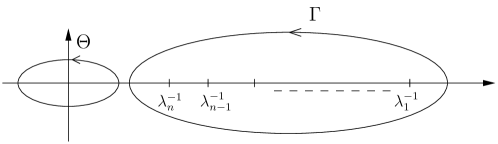
Figure 5: The contours $\Gamma$ and $\Theta$ in the definition of ${\rm K}_{N}(x,y)$

Remark 4.1.

In [4, On], it is assumed that $q$ satisfies an extra restriction so that the associated operator ${\rm K}_{N}$ is trace class on the semi-infinite intervals $(s,+\infty)$. Since we are here only interested in establishing a local uniform convergence for ${\rm K}_{N}(x,y)$, such restrictions are not necessary. See also [HHN-preprint, Remark 4.3].

In the remaining of this section, we assume that the framework (assumptions and notations) of Theorem 5 holds true. We then set

$$\widetilde{\rm K}_{N}(x,y)=\frac{1}{N^{3/4}\sigma_{N}}{\rm K}_{N}\left(\mathfrak{a}_{N}+\frac{x}{N^{3/4}\sigma_{N}},\mathfrak{a}_{N}+\frac{y}{N^{3/4}\sigma_{N}}\right),$$ (4.2)

and, in order to establish Theorem 5, focus on the proof of the uniform convergence

$$\sup_{x,y\in[-s,s]}\Big{|}\widetilde{\rm K}_{N}(x,y)-{\rm K}^{(\tau)}_{\rm Pe}(x,y)\Big{|}\xrightarrow[N\to\infty]{}0$$ (4.3)

for every fixed $s>0$.

Notations and conventions:

• We denote by $B(z,\rho)$ the open disc in $\mathbb{C}$ with center $z\in\mathbb{C}$ and radius $\rho>0$.

• By convention, we shall use at several instances a constant $C$ which depends neither on $N$ nor on $x,y\in[-s,s]$, but may depend on $s$, and whose exact value may change from one ligne to another.

• If a contour $\Gamma$ is parametrized by $\gamma:I\rightarrow\Gamma$ for some interval $I\subset\mathbb{R}$, then for every map $h:\Gamma\rightarrow\mathbb{C}$ we set

  $$\int_{\Gamma}h(z)|{\rm d}z|=\int_{I}h\circ\gamma(t)\,|\gamma^{\prime}(t)|{\rm d}t$$

  when it does make sense. In particular, ${\oint}_{\Gamma}|{\rm d}z|$ is the length of a closed contour $\Gamma$.

4.1 Preparation

It follows from (4.1) and (4.2), by setting $q=\mathfrak{c}_{N}$, that

$$\widetilde{\rm K}_{N}(x,y)=\frac{N^{1/4}}{(2i\pi)^{2}\sigma_{N}}\oint_{\Gamma}{\rm d}z\oint_{\Theta}{\rm d}w\,\frac{1}{w-z}\,e^{-\frac{N^{1/4}}{\sigma_{N}}x(z-\mathfrak{c}_{N})+\frac{N^{1/4}}{\sigma_{N}}y(w-\mathfrak{c}_{N})}e^{Nf_{N}(z)-Nf_{N}(w)},$$ (4.4)

where we introduced the map

$$f_{N}(z)=-\mathfrak{a}_{N}(z-\mathfrak{c}_{N})+\log(z)-\frac{1}{N}\sum_{j=1}^{n}\log(1-\lambda_{j}z)\ .$$ (4.5)

Notice the functions $\exp(f_{N})$, $\mathfrak{Re}f_{N}$, and the derivatives $f_{N}^{(k)}$ ($k\geqslant 1$) are well-defined on $\mathbb{C}\setminus\{0,\lambda_{1}^{-1},\ldots,\lambda_{n}^{-1}\}$. However, one needs to specify an appropriate determination of the complex logarithm in order to define $f_{N}$ properly. By Assumption 2 and the regularity condition (2.22), there exists $\varepsilon>0$ such that $\lambda_{j}^{-1}\in(0,+\infty)\setminus B(\mathfrak{c},\varepsilon)$ for every $1\leqslant j\leqslant n$ and every $N$ large enough. As a consequence, if we introduce the compact set

$${\mathcal{K}}=\left(\left[\inf_{N}\frac{1}{\lambda_{n}},\sup_{N}\frac{1}{\lambda_{1}}\right]\setminus B(\mathfrak{c},\varepsilon)\right)\cup\{0\}\ ,$$ (4.6)

then on every simply connected open subset of $\mathbb{C}\setminus\mathcal{K}$ one can find a determination of the logarithm so that $f_{N}$ is well-defined and holomorphic there.

Recalling the definition (2.23) of $g_{N}$, an essential observation is that

$$f_{N}^{\prime}(z)=g_{N}(z)-\mathfrak{a}_{N}\ .$$ (4.7)

As a consequence, we have for every $k\geqslant 1$,

$$f_{N}^{(k+1)}(z)=g_{N}^{(k)}(z)\ .$$ (4.8)

In particular, since $\mathfrak{a}_{N}=g_{N}(\mathfrak{c}_{N})$ by definition, the decay assumption (2.24) and Proposition 4 provide

$$f^{\prime}(\mathfrak{c}_{N}) =0\ ,$$ (4.9)

$$\sqrt{N}f_{N}^{\prime\prime}(\mathfrak{c}_{N}) \xrightarrow[N\to\infty]{}\tau\ ,$$ (4.10)

$$f^{(3)}(\mathfrak{c}_{N}) =0\ ,$$ (4.11)

$$f_{N}^{(4)}(\mathfrak{c}_{N}) \xrightarrow[N\to\infty]{}g^{(3)}(\mathfrak{c})>0\ .$$ (4.12)

By performing a Taylor expansion of $f_{N}$ near $\mathfrak{c}_{N}$ in (4.4), one can already guess from (4.9)–(4.12) and a change of variables that the Pearcey kernel should appear in the large $N$ limit, at least if one restricts the contours $\Gamma$ and $\Theta$ to a neighbourhood of $\mathfrak{c}_{N}$ (see also [HHN-esaim-preprint] for a more detailed heuristic, which may serve as a guideline for the forthcoming proof). In a first step, we provide precise estimates in order to prove that claim, see Section 4.2. In a second step, we prove that the contribution coming from the pieces of contour away from $\mathfrak{c}_{N}$ are exponentially negligible, see Section 4.3. To do so, we establish the existence of appropriate contours in the same fashion as in [HHN-preprint]. This will enable us to conclude.

Notice that one of the key arguments to assert the existence of appropriate contours is the maximum principle for subharmonic functions. This argument only appears in the proof of Lemma 4.9, which is similar to the proof of [HHN-preprint, Lemma 4.11] and hence omitted. The interested reader may refer to [HHN-preprint] for more details.

4.2 Step 1: Local analysis around $\mathfrak{c}_{N}$

We start with a quantitative Taylor expansion for $f_{N}$ near $\mathfrak{c}_{N}$.

Lemma 4.2.

There exists $\rho_{0}>0$ and $\Delta=\Delta(\rho_{0})>0$ independent of $N$ such that for every $N$ large enough, $B(\mathfrak{c}_{N},\rho_{0})\subset\mathbb{C}\setminus{\mathcal{K}}$ and, whatever the analytic representation of $f_{N}$ on $B(\mathfrak{c}_{N},\rho_{0})$, we have for every $z\in B(\mathfrak{c}_{N},\rho_{0})$

$$\big{|}f_{N}(z)-f_{N}(\mathfrak{c}_{N})-\frac{1}{2}g^{\prime}_{N}(\mathfrak{c}_{N})(z-\mathfrak{c}_{N})^{2}-\frac{1}{4!}g^{(3)}_{N}(\mathfrak{c}_{N})(z-\mathfrak{c}_{N})^{4}\big{|}\leqslant\Delta|z-\mathfrak{c}_{N}|^{5}.$$

In particular, since $g_{N}^{\prime}(\mathfrak{c}_{N})$ is real, for every $z\in B(\mathfrak{c}_{N},\rho_{0})$,

$$\big{|}\mathfrak{Re}f_{N}(z)-\mathfrak{Re}f_{N}(\mathfrak{c}_{N})-\frac{1}{2}g^{\prime}_{N}(\mathfrak{c}_{N})\mathfrak{Re}(z-\mathfrak{c}_{N})^{2}-\frac{1}{4!}g^{(3)}_{N}(\mathfrak{c}_{N})\mathfrak{Re}(z-\mathfrak{c}_{N})^{4}\big{|}\leqslant\Delta|z-\mathfrak{c}_{N}|^{5}.$$

Proof.

Choose $\rho_{0}$ such that $B(\mathfrak{c},2\rho_{0})\subset\mathbb{C}\setminus\mathcal{K}$. The convergence $\mathfrak{c}_{N}\to\mathfrak{c}$ then yields $B(\mathfrak{c}_{N},\rho_{0})\subset B(\mathfrak{c},2\rho_{0})\subset\mathbb{C}\setminus\mathcal{K}$ for every $N$ large enough. By using (4.8)–(4.11) and performing a Taylor expansion for $f_{N}$ around $\mathfrak{c}_{N}$, we obtain

$$\big{|}f_{N}(z)-f_{N}(\mathfrak{c}_{N})-\frac{1}{2}g^{\prime}_{N}(\mathfrak{c}_{N})(z-\mathfrak{c}_{N})^{2}-\frac{1}{4!}g^{(3)}_{N}(\mathfrak{c}_{N})(z-\mathfrak{c}_{N})^{4}\big{|}$$

$$= \quad\big{|}f_{N}(z)-f_{N}(\mathfrak{c}_{N})-\frac{1}{2}f^{\prime\prime}_{N}(\mathfrak{c}_{N})(z-\mathfrak{c}_{N})^{2}-\frac{1}{4!}f^{(4)}_{N}(\mathfrak{c}_{N})(z-\mathfrak{c}_{N})^{4}\big{|}$$

$$\leqslant \quad\frac{1}{5!}|z-\mathfrak{c}_{N}|^{5}\max_{B(\mathfrak{c},2\rho_{0})}|f_{N}^{(5)}|\ ,$$

provided that $z\in B(\mathfrak{c}_{N},\rho_{0})$ and $N$ is sufficiently large. Moreover, since $f_{N}^{(5)}=g_{N}^{(4)}$ converges uniformly on $B(\mathfrak{c},2\rho_{0})$ to $g^{(4)}$ which is bounded there, the existence of $\Delta=\Delta(\rho_{0})$ independent of $N$ follows. ∎

From now, we let $\rho>0$ be small enough so that $0<\rho<\rho_{0}$ and

$$\frac{g_{N}^{(3)}(\mathfrak{c}_{N})}{4!}-\Delta\rho\geqslant\frac{1}{2}\,\frac{g^{(3)}(\mathfrak{c})}{4!}$$ (4.13)

We introduce the contours

$$\Upsilon^{+}_{o} =\left\{\mathfrak{c}_{N}+N^{-1/4}e^{-i\theta}:\quad\theta\in[-\pi/4,\pi/4]\right\}\ ,$$ (4.14)

$$\Upsilon^{+}_{\times} =\left\{\mathfrak{c}_{N}-te^{i\pi/4}:\quad t\in[-\rho,-N^{-1/4}]\right\}\cup\left\{\mathfrak{c}_{N}+te^{-i\pi/4}:\quad t\in[N^{-1/4},\rho]\right\}\ ,$$ (4.15)

$$\Upsilon^{-}_{o} =\left\{\mathfrak{c}_{N}-N^{-1/4}e^{-i\theta}:\quad\theta\in[-\pi/4,\pi/4]\right\}\ ,$$ (4.16)

$$\Upsilon^{-}_{\times} =\left\{\mathfrak{c}_{N}+te^{i\pi/4}:\quad t\in[-\rho,-N^{-1/4}]\right\}\cup\left\{\mathfrak{c}_{N}+te^{3i\pi/4}:\quad t\in[N^{-1/4},\rho]\right\}\ .$$ (4.17)

The orientations of these contours are specified by letting the parameters $\theta$ and $t$ increase in their definition domains. We also introduce

$$\Upsilon_{*} =\Upsilon^{+}_{o}\cup\Upsilon^{+}_{\times}\cup\Upsilon^{-}_{o}\cup\Upsilon^{-}_{\times}\ ,$$ (4.18)

$$\Xi_{*} =\left\{\mathfrak{c}_{N}+te^{i\pi/2}:\quad t\in[-\rho,\rho]\right\}.$$ (4.19)

Similarly, the orientation of contour $\Xi_{*}$ is specified by letting $t$ increase in its definition domain.

We now establish the following estimate which essentially allows to replace $f_{N}$ by its Taylor expansion around $\mathfrak{c}_{N}$ in the double integral over the contours $\Upsilon_{*}$ and $\Xi_{*}$.

Lemma 4.3.

For every $s>0$, the following quantity

$$\frac{N^{1/4}}{(2i\pi)^{2}\sigma_{N}}\int_{\Upsilon_{*}}{\rm d}z\int_{\Xi_{*}}{\rm d}w\,\frac{1}{w-z}\,e^{-N^{1/4}x\frac{(z-\mathfrak{c}_{N})}{\sigma_{N}}+N^{1/4}y\frac{(w-\mathfrak{c}_{N})}{\sigma_{N}}}$$ (4.20)

$$\times\left\{e^{Nf_{N}(z)-Nf_{N}(w)}-e^{N\frac{g_{N}^{\prime}(\mathfrak{c}_{N})}{2}(z-\mathfrak{c}_{N})^{2}+N\frac{g_{N}^{(3)}(\mathfrak{c}_{N})}{4!}(z-\mathfrak{c}_{N})^{4}-N\frac{g_{N}^{\prime}(\mathfrak{c}_{N})}{2}(w-\mathfrak{c}_{N})^{2}-N\frac{g_{N}^{(3)}(\mathfrak{c}_{N})}{4!}(w-\mathfrak{c}_{N})^{4}}\right\}$$

converges to zero as $N\to\infty$, uniformly in $x,y\in[-s,s]$.

Proof.

Let $s>0$ be fixed, and set for convenience

$$D_{N}(z,w)=e^{Nf_{N}(z)-Nf_{N}(w)}\\ -e^{N\frac{g_{N}^{\prime}(\mathfrak{c}_{N})}{2}(z-\mathfrak{c}_{N})^{2}+N\frac{g_{N}^{(3)}(\mathfrak{c}_{N})}{4!}(z-\mathfrak{c}_{N})^{4}-N\frac{g_{N}^{\prime}(\mathfrak{c}_{N})}{2}(w-\mathfrak{c}_{N})^{2}-N\frac{g_{N}^{(3)}(\mathfrak{c}_{N})}{4!}(w-\mathfrak{c}_{N})^{4}}\ ,$$

so that it amounts to prove that

$$N^{1/4}\sup_{x,y\in[-s,s]}\Bigg{|}\int_{\Upsilon_{*}}{\rm d}z\int_{\Xi_{*}}{\rm d}w\,\frac{1}{w-z}\,e^{-N^{1/4}x\frac{(z-\mathfrak{c}_{N})}{\sigma_{N}}+N^{1/4}y\frac{(w-\mathfrak{c}_{N})}{\sigma_{N}}}D_{N}(z,w)\Bigg{|}$$ (4.21)

vanishes as $N\to\infty$.

First, by definition of the contours (4.14)–(4.19), we have the bound

$$\frac{1}{|z-w|}\leqslant\sqrt{2}\,N^{1/4}$$

for every $z\in\Upsilon_{*}$ and $w\in\Xi_{*}$. As a consequence,

$$N^{1/4}\Big{|}\int_{\Upsilon_{*}}{\rm d}z\int_{\Xi_{*}}{\rm d}w\,\frac{1}{w-z}\,e^{-N^{1/4}x\frac{(z-\mathfrak{c}_{N})}{\sigma_{N}}+N^{1/4}y\frac{(w-\mathfrak{c}_{N})}{\sigma_{N}}}D_{N}(z,w)\Big{|}$$

$$\leqslant \quad\sqrt{2N}\int_{\Upsilon_{*}}|{\rm d}z|\int_{\Xi_{*}}|{\rm d}w|\,e^{-N^{1/4}x\frac{\mathfrak{Re}(z-\mathfrak{c}_{N})}{\sigma_{N}}+N^{1/4}y\frac{\mathfrak{Re}(w-\mathfrak{c}_{N})}{\sigma_{N}}}\Big{|}D_{N}(z,w)\Big{|}\ .$$ (4.22)

Next, we use the following elementary inequality,

$$|e^{u}-e^{v}| = e^{\mathfrak{Re}(v)}|e^{(u-v)}-1|$$ (4.23)

$$\leqslant e^{\mathfrak{Re}(v)}\sum_{k\geqslant 1}\frac{|u-v|^{k}}{k!}\ \leqslant\ |u-v|e^{\mathfrak{Re}(v)+|u-v|}\ ,$$

which holds true for every $u,v\in\mathbb{C}$. By specializing it to

$$u = Nf_{N}(z)-Nf_{N}(w)=N(f_{N}(z)-f_{N}(\mathfrak{c}_{N}))-N(f_{N}(w)-f_{N}(\mathfrak{c}_{N}))\ ,$$

$$v = N\frac{g_{N}^{\prime}(\mathfrak{c}_{N})}{2}(z-\mathfrak{c}_{N})^{2}+N\frac{g_{N}^{(3)}(\mathfrak{c}_{N})}{4!}(z-\mathfrak{c}_{N})^{4}$$

$$\qquad-N\frac{g_{N}^{\prime}(\mathfrak{c}_{N})}{2}(w-\mathfrak{c}_{N})^{2}-N\frac{g_{N}^{(3)}(\mathfrak{c}_{N})}{4!}(w-\mathfrak{c}_{N})^{4}\ ,$$

where $z\in\Upsilon_{*}$ and $w\in\Xi_{*}$, so that Lemma 4.2 yields $|u-v|\leqslant N\Delta(|z-\mathfrak{c}_{N}|^{5}+|w-\mathfrak{c}_{N}|^{5})$ , we obtain

$$\Big{|}D_{N}(z,w)\Big{|} \leqslant N\Delta(|z-\mathfrak{c}_{N}|^{5}+|w-\mathfrak{c}_{N}|^{5})$$

$$\quad\times\,e^{N\frac{g_{N}^{\prime}(\mathfrak{c}_{N})}{2}\mathfrak{Re}(z-\mathfrak{c}_{N})^{2}+N\frac{g_{N}^{(3)}(\mathfrak{c}_{N})}{4!}\mathfrak{Re}(z-\mathfrak{c}_{N})^{4}+N\Delta|z-\mathfrak{c}_{N}|^{5}}$$

$$\qquad\times\,e^{-N\frac{g_{N}^{\prime}(\mathfrak{c}_{N})}{2}\mathfrak{Re}(w-\mathfrak{c}_{N})^{2}-N\frac{g_{N}^{(3)}(\mathfrak{c}_{N})}{4!}\mathfrak{Re}(w-\mathfrak{c}_{N})^{4}+N\Delta|w-\mathfrak{c}_{N}|^{5}}.$$

As a consequence, it follows

$$\Delta^{-1}\int_{\Upsilon_{*}}|{\rm d}z|\int_{\Xi_{*}}|{\rm d}w|\,e^{-N^{1/4}x\frac{\mathfrak{Re}(z-\mathfrak{c}_{N})}{\sigma_{N}}+N^{1/4}y\frac{\mathfrak{Re}(w-\mathfrak{c}_{N})}{\sigma_{N}}}\Big{|}D_{N}(z,w)\Big{|}$$

$$\leqslant \int_{\Upsilon_{*}}N|z-\mathfrak{c}_{N}|^{5}e^{-N^{1/4}x\frac{\mathfrak{Re}(z-\mathfrak{c}_{N})}{\sigma_{N}}+N\frac{g_{N}^{\prime}(\mathfrak{c}_{N})}{2}\mathfrak{Re}(z-\mathfrak{c}_{N})^{2}+N\frac{g_{N}^{(3)}(\mathfrak{c}_{N})}{4!}\mathfrak{Re}(z-\mathfrak{c}_{N})^{4}+N\Delta|z-\mathfrak{c}_{N}|^{5}}|{\rm d}z|$$

$$\qquad\times\int_{\Xi_{*}}e^{N^{1/4}y\frac{\mathfrak{Re}(w-\mathfrak{c}_{N})}{\sigma_{N}}-N\frac{g_{N}^{\prime}(\mathfrak{c}_{N})}{2}\mathfrak{Re}(w-\mathfrak{c}_{N})^{2}-N\frac{g_{N}^{(3)}(\mathfrak{c}_{N})}{4!}\mathfrak{Re}(w-\mathfrak{c}_{N})^{4}+N\Delta|w-\mathfrak{c}_{N}|^{5}}|{\rm d}w|$$

$$\quad+\int_{\Upsilon_{*}}e^{-N^{1/4}x\frac{\mathfrak{Re}(z-\mathfrak{c}_{N})}{\sigma_{N}}+N\frac{g_{N}^{\prime}(\mathfrak{c}_{N})}{2}\mathfrak{Re}(z-\mathfrak{c}_{N})^{2}+N\frac{g_{N}^{(3)}(\mathfrak{c}_{N})}{4!}\mathfrak{Re}(z-\mathfrak{c}_{N})^{4}+N\Delta|z-\mathfrak{c}_{N}|^{5}}|{\rm d}z|$$

$$\qquad\times\int_{\Xi_{*}}N|w-\mathfrak{c}_{N}|^{5}e^{N^{1/4}y\frac{\mathfrak{Re}(w-\mathfrak{c}_{N})}{\sigma_{N}}-N\frac{g_{N}^{\prime}(\mathfrak{c}_{N})}{2}\mathfrak{Re}(w-\mathfrak{c}_{N})^{2}-N\frac{g_{N}^{(3)}(\mathfrak{c}_{N})}{4!}\mathfrak{Re}(w-\mathfrak{c}_{N})^{4}+N\Delta|w-\mathfrak{c}_{N}|^{5}}|{\rm d}w|.$$

We now handle the integrals over each piece of contour separately.

First, consider the integrals over the contour $\Xi_{*}$. By definition $w\in\Xi_{*}$ if and only if there exists $t\in[-\rho,\rho]$ such that $w=\mathfrak{c}_{N}+it$. Thus,

$$\mathfrak{Re}(w-\mathfrak{c}_{N})=0,\qquad\mathfrak{Re}(w-\mathfrak{c}_{N})^{2}=-t^{2},\qquad\mathfrak{Re}(w-\mathfrak{c}_{N})^{4}=t^{4},\qquad|w-\mathfrak{c}_{N}|^{5}=|t|^{5}.$$

For $N$ large enough this yields, together with (4.13),

$$\int_{\Xi_{*}}e^{N^{1/4}y\frac{\mathfrak{Re}(w-\mathfrak{c}_{N})}{\sigma_{N}}-N\frac{g_{N}^{\prime}(\mathfrak{c}_{N})}{2}\mathfrak{Re}(w-\mathfrak{c}_{N})^{2}-N\frac{g_{N}^{(3)}(\mathfrak{c}_{N})}{4!}\mathfrak{Re}(w-\mathfrak{c}_{N})^{4}+N\Delta|w-\mathfrak{c}_{N}|^{5}}|{\rm d}w|$$ (4.25)

$$= \int_{-\rho}^{\rho}e^{N\frac{g_{N}^{\prime}(\mathfrak{c}_{N})}{2}t^{2}-N\frac{g_{N}^{(3)}(\mathfrak{c}_{N})}{4!}t^{4}+N\Delta|t|^{5}}{\rm d}t$$

$$\leqslant \int_{-\rho}^{\rho}e^{N\frac{g_{N}^{\prime}(\mathfrak{c}_{N})}{2}t^{2}-Nt^{4}\left(\frac{g_{N}^{(3)}(\mathfrak{c}_{N})}{4!}-\rho\Delta\right)}{\rm d}t$$

$$\leqslant \int_{-\rho}^{\rho}e^{N\frac{g_{N}^{\prime}(\mathfrak{c}_{N})}{2}t^{2}-N\xi t^{4}}{\rm d}t$$

$$= \frac{1}{N^{1/4}}\int_{-\rho N^{1/4}}^{\rho N^{1/4}}e^{\sqrt{N}\frac{g_{N}^{\prime}(\mathfrak{c}_{N})}{2}t^{2}-\xi t^{4}}{\rm d}t$$

$$\leqslant \frac{1}{N^{1/4}}\int_{-\infty}^{+\infty}e^{\sqrt{N}\frac{g_{N}^{\prime}(\mathfrak{c}_{N})}{2}t^{2}-\xi t^{4}}{\rm d}t\quad\leqslant\quad\frac{C}{N^{1/4}}$$

where we set for convenience

$$\xi\ =\ \frac{1}{2}\,\frac{g^{(3)}(\mathfrak{c})}{4!}\,>\ 0\,.$$

For the last estimate, we have used the decay assumption $\sqrt{N}\,g_{N}^{\prime}(\mathfrak{c}_{N})\to\kappa\in\mathbb{R}$. Similarly,

$$\int_{\Xi_{*}}N|w-\mathfrak{c}_{N}|^{5}e^{N^{1/4}y\frac{\mathfrak{Re}(w-\mathfrak{c}_{N})}{\sigma_{N}}-N\frac{g_{N}^{\prime}(\mathfrak{c}_{N})}{2}\mathfrak{Re}(w-\mathfrak{c}_{N})^{2}-N\frac{g_{N}^{(3)}(\mathfrak{c}_{N})}{4!}\mathfrak{Re}(w-\mathfrak{c}_{N})^{4}+N\Delta|w-\mathfrak{c}_{N}|^{5}}|{\rm d}w|$$

$$\quad=\quad N\int_{-\rho}^{\rho}|t|^{5}e^{N\frac{g_{N}^{\prime}(\mathfrak{c}_{N})}{2}t^{2}-N\frac{g_{N}^{(3)}(\mathfrak{c}_{N})}{4!}t^{4}+N\Delta|t|^{5}}{\rm d}t$$

$$\quad\leqslant\quad N\int_{-\rho}^{\rho}|t|^{5}e^{N\frac{g_{N}^{\prime}(\mathfrak{c}_{N})}{2}t^{2}-N\xi t^{4}}{\rm d}t$$

$$\quad=\quad\frac{1}{\sqrt{N}}\int_{-\rho N^{1/4}}^{\rho N^{1/4}}|t|^{5}e^{\sqrt{N}\frac{g_{N}^{\prime}(\mathfrak{c}_{N})}{2}t^{2}-\xi t^{4}}{\rm d}t\quad\leqslant\quad\frac{C}{\sqrt{N}}\ .$$ (4.26)

Next, we turn to the integrals over the contours $\Upsilon^{+}_{\times}$ and $\Upsilon^{-}_{\times}$. By definition $z\in\Upsilon^{+}_{\times}$, resp. $z\in\Upsilon^{-}_{\times}$, if and only if there exists $t\in[N^{-1/4},\rho]$ such that $z=\mathfrak{c}_{N}+e^{\pm i\pi/4}t$, resp. $z=\mathfrak{c}_{N}-e^{\pm i\pi/4}t$, so that in both cases we have

$$|\mathfrak{Re}(z-\mathfrak{c}_{N})|\leqslant t,\qquad\mathfrak{Re}(z-\mathfrak{c}_{N})^{2}=0,\qquad\mathfrak{Re}(z-\mathfrak{c}_{N})^{4}=-t^{4},\qquad|z-\mathfrak{c}_{N}|^{5}=t^{5}.$$

As a consequence, for every $x\in[-s,s]$,

$$\int_{\Upsilon^{+}_{\times}\cup\Upsilon^{-}_{\times}}e^{-N^{1/4}x\frac{\mathfrak{Re}(z-\mathfrak{c}_{N})}{\sigma_{N}}+N\frac{g_{N}^{\prime}(\mathfrak{c}_{N})}{2}\mathfrak{Re}(z-\mathfrak{c}_{N})^{2}+N\frac{g_{N}^{(3)}(\mathfrak{c}_{N})}{4!}\mathfrak{Re}(z-\mathfrak{c}_{N})^{4}+N\Delta|z-\mathfrak{c}_{N}|^{5}}|{\rm d}z|$$

$$\quad\leqslant\quad 4\int_{N^{-1/4}}^{\rho}e^{N^{1/4}\frac{st}{\sigma_{N}}-N\frac{g_{N}^{(3)}(\mathfrak{c}_{N})}{4!}t^{4}+N\Delta|t|^{5}}{\rm d}t$$

$$\quad\leqslant\quad 4\int_{N^{-1/4}}^{\rho}e^{N^{1/4}\frac{st}{\sigma_{N}}-N\xi t^{4}}{\rm d}t$$

$$\quad=\quad\frac{4}{N^{1/4}}\int_{1}^{\rho N^{1/4}}e^{\frac{st}{\sigma_{N}}-\xi t^{4}}{\rm d}t\quad\leqslant\quad\frac{C}{N^{1/4}}$$ (4.27)

where the last inequality follows from the fact that $\liminf_{N}\sigma_{N}>0$. Similarly,

$$\int_{\Upsilon^{+}_{\times}\cup\Upsilon^{-}_{\times}}N|z-\mathfrak{c}_{N}|^{5}e^{-N^{1/4}x\frac{\mathfrak{Re}(z-\mathfrak{c}_{N})}{\sigma_{N}}+N\frac{g_{N}^{\prime}(\mathfrak{c}_{N})}{2}\mathfrak{Re}(z-\mathfrak{c}_{N})^{2}+N\frac{g_{N}^{(3)}(\mathfrak{c}_{N})}{4!}\mathfrak{Re}(z-\mathfrak{c}_{N})^{4}+N\Delta|z-\mathfrak{c}_{N}|^{5}}|{\rm d}z|$$

$$\quad\leqslant\quad 4N\int_{N^{-1/4}}^{\rho}t^{5}e^{N^{1/4}\frac{st}{\sigma_{N}}-N\frac{g_{N}^{(3)}(\mathfrak{c}_{N})}{4!}t^{4}+N\Delta|t|^{5}}{\rm d}t$$

$$\quad\leqslant\quad 4N\int_{N^{-1/4}}^{\rho}t^{5}e^{N^{1/4}\frac{st}{\sigma_{N}}-N\xi t^{4}}{\rm d}t$$

$$\quad=\quad\frac{4}{\sqrt{N}}\int_{1}^{\rho N^{1/4}}t^{5}e^{\frac{st}{\sigma_{N}}-\xi t^{4}}{\rm d}t\quad\leqslant\quad\frac{C}{\sqrt{N}}\ .$$ (4.28)

Finally, we consider the integrals over the contours $\Upsilon^{+}_{o}$ and $\Upsilon^{-}_{o}$. By definition $z\in\Upsilon^{+}_{o}\cup\Upsilon^{-}_{o}$ if and only if there exists $\theta\in[-\pi/4,\pi/4]$ such that $z=\mathfrak{c}_{N}\pm N^{-1/4}e^{i\theta}$, and hence

$$|\mathfrak{Re}(z-\mathfrak{c}_{N})|\leqslant N^{-1/4},\qquad|\mathfrak{Re}(z-\mathfrak{c}_{N})^{2}|\leqslant N^{-1/2},\qquad|\mathfrak{Re}(z-\mathfrak{c}_{N})^{4}|\leqslant N^{-1},\qquad|z-\mathfrak{c}_{N}|^{5}\leqslant N^{-5/4}.$$

As a consequence, for every $x\in[-s,s]$,

$$\int_{\Upsilon^{+}_{o}\cup\Upsilon^{-}_{o}}e^{-N^{1/4}x\frac{\mathfrak{Re}(z-\mathfrak{c}_{N})}{\sigma_{N}}+N\frac{g_{N}^{\prime}(\mathfrak{c}_{N})}{2}\mathfrak{Re}(z-\mathfrak{c}_{N})^{2}+N\frac{g_{N}^{(3)}(\mathfrak{c}_{N})}{4!}\mathfrak{Re}(z-\mathfrak{c}_{N})^{4}+N\Delta|z-\mathfrak{c}_{N}|^{5}}|{\rm d}z|$$

$$\quad\leqslant\quad e^{\frac{s}{\sigma_{N}}+\sqrt{N}g_{N}^{\prime}(\mathfrak{c}_{N})+g_{N}^{(3)}(\mathfrak{c}_{N})+\frac{\Delta}{N^{1/4}}}\int_{\Upsilon^{+}_{o}\cup\Upsilon^{-}_{o}}|{\rm d}z|$$

$$\quad=\quad\frac{\pi}{N^{1/4}}\,e^{\frac{s}{\sigma_{N}}+\sqrt{N}g_{N}^{\prime}(\mathfrak{c}_{N})+g_{N}^{(3)}(\mathfrak{c}_{N})+\frac{\Delta}{N^{1/4}}}\quad\leqslant\quad\frac{C}{N^{1/4}}\ ,$$ (4.29)

where for the last estimate, we used the fact that $\liminf_{N}\sigma_{N}>0$, the decay assumption $\sqrt{N}\,g_{N}^{\prime}(\mathfrak{c}_{N})\to\kappa\in\mathbb{R}$ and the convergence $g_{N}^{(3)}(\mathfrak{c}_{N})\to g^{(3)}(\mathfrak{c})$. Similarly,

$$\int_{\Upsilon^{+}_{o}\cup\Upsilon^{-}_{o}}N|z-\mathfrak{c}_{N}|^{5}e^{-N^{1/4}x\frac{\mathfrak{Re}(z-\mathfrak{c}_{N})}{\sigma_{N}}+N\frac{g_{N}^{\prime}(\mathfrak{c}_{N})}{2}\mathfrak{Re}(z-\mathfrak{c}_{N})^{2}+N\frac{g_{N}^{(3)}(\mathfrak{c}_{N})}{4!}\mathfrak{Re}(z-\mathfrak{c}_{N})^{4}+N\Delta|z-\mathfrak{c}_{N}|^{5}}|{\rm d}z|$$

$$\quad\leqslant\quad\frac{\pi}{\sqrt{N}}\,e^{\frac{s}{\sigma_{N}}+\sqrt{N}g_{N}^{\prime}(\mathfrak{c}_{N})+g_{N}^{(3)}(\mathfrak{c}_{N})+\frac{\Delta}{N^{1/4}}}\quad\leqslant\quad\frac{C}{\sqrt{N}}\ .$$ (4.30)

By gathering (LABEL:A1)–(4.2), we thus obtain the estimate

$$\Delta^{-1}\int_{\Upsilon_{*}}|{\rm d}z|\int_{\Xi_{*}}|{\rm d}w|\,e^{-N^{1/4}x\frac{\mathfrak{Re}(z-\mathfrak{c}_{N})}{\sigma_{N}}+N^{1/4}y\frac{\mathfrak{Re}(w-\mathfrak{c}_{N})}{\sigma_{N}}}\Big{|}D_{N}(z,w)\Big{|}\leqslant\frac{C}{N^{3/4}}.$$

Combined together with (4.2), this finally yields

$$N^{1/4}\sup_{x,y\in[-s,s]}\Bigg{|}\int_{\Upsilon_{*}}{\rm d}z\int_{\Xi_{*}}{\rm d}w\,\frac{1}{w-z}\,e^{-N^{1/4}x\frac{(z-\mathfrak{c}_{N})}{\sigma_{N}}+N^{1/4}y\frac{(w-\mathfrak{c}_{N})}{\sigma_{N}}}D_{N}(z,w)\Bigg{|}\leqslant\frac{C}{N^{1/4}}\ .$$

Hence, (4.21) is proved, which in turn implies (4.20). Proof of Lemma 4.3 is therefore complete. ∎

The next estimate completes the previous lemma by showing one can replace the constant $Ng^{\prime}_{N}(\mathfrak{c}_{N})$ in (4.20) by $-\sqrt{N}\tau/\sigma_{N}^{2}$, and that the resulting kernel is the Pearcey kernel, up to a negligible correction term.

Lemma 4.4.

For every $s>0$,

$$\frac{N^{1/4}}{(2i\pi)^{2}\sigma_{N}}\int_{\Upsilon_{*}}{\rm d}z\int_{\Xi_{*}}{\rm d}w\,\frac{1}{w-z}\,e^{-N^{1/4}x\frac{(z-\mathfrak{c}_{N})}{\sigma_{N}}+N^{1/4}y\frac{(w-\mathfrak{c}_{N})}{\sigma_{N}}}\\ \times e^{N\frac{g_{N}^{\prime}(\mathfrak{c}_{N})}{2}(z-\mathfrak{c}_{N})^{2}+N\frac{g_{N}^{(3)}(\mathfrak{c}_{N})}{4!}(z-\mathfrak{c}_{N})^{4}-N\frac{g_{N}^{\prime}(\mathfrak{c}_{N})}{2}(w-\mathfrak{c}_{N})^{2}-N\frac{g_{N}^{(3)}(\mathfrak{c}_{N})}{4!}(w-\mathfrak{c}_{N})^{4}}$$

converges as $N\to\infty$ towards ${\rm K}_{\rm Pe}^{(\tau)}(x,y)$, uniformly in $x,y\in[-s,s]$.

Proof.

Let $s>0$ be fixed and recall the definition (2.21) of ${\rm K}_{\rm Pe}^{(\tau)}(x,y)$. We first show that, uniformly in $x,y\in[-s,s]$, as $N\to\infty$,

$${\rm K}_{\rm Pe}^{(\tau)}(x,y)=\int_{\Sigma\,\cap\,\left\{|z|\leqslant\frac{N^{1/4}\rho}{\sigma_{N}}\right\}}{\rm d}z\int_{-iN^{1/4}\rho/\sigma_{N}}^{\,iN^{1/4}\rho/\sigma_{N}}{\rm d}w\,\frac{1}{w-z}\,e^{-xz-\frac{\tau}{2}z^{2}+\frac{z^{4}}{4}+yw+\frac{\tau}{2}w^{2}-\frac{w^{4}}{4}}\\ +{\mathcal{O}}\left({\frac{1}{N^{1/4}}}\right)\ .$$ (4.31)

Indeed, keeping in mind that the sequence $(\sigma_{N})$ is bounded, it follows from the definition (2.19) of $\Sigma$ together with simple estimates that for every $x,y\in[-s,s]$,

$$\Bigg{|}\int_{\Sigma\,\cap\,\left\{|z|\geqslant\frac{N^{1/4}\rho}{\sigma_{N}}\right\}}{\rm d}z\int_{-i\infty}^{\,i\infty}{\rm d}w\,\frac{1}{w-z}\,e^{-xz-\frac{\tau}{2}z^{2}+\frac{z^{4}}{4}+yw+\frac{\tau}{2}w^{2}-\frac{w^{4}}{4}}\Bigg{|}\\ \leqslant\quad\frac{\sqrt{2}\,\sigma_{N}}{N^{1/4}\rho}\,4\int_{N^{1/4}\rho/\sigma_{N}}^{+\infty}e^{s|t|-\frac{t^{4}}{4}}{\rm d}t\int_{-\infty}^{+\infty}e^{-\frac{\tau}{2}u^{2}-\frac{u^{4}}{4}}{\rm d}u\quad\leqslant\frac{C}{N^{1/4}}\ ,$$

and

$$\Bigg{|}\int_{\Sigma}{\rm d}z\left(\int_{-i\infty}^{-iN^{1/4}\rho/\sigma_{N}}+\int_{iN^{1/4}\rho/\sigma_{N}}^{i\infty}\right){\rm d}w\,\frac{1}{w-z}\,e^{-xz-\frac{\tau}{2}z^{2}+\frac{z^{4}}{4}+yw+\frac{\tau}{2}w^{2}-\frac{w^{4}}{4}}\Bigg{|}\\ \leqslant\quad\frac{\sqrt{2}\,\sigma_{N}}{N^{1/4}\rho}\left(4\int_{1}^{+\infty}e^{s|t|-\frac{t^{4}}{4}}{\rm d}t+\frac{1}{\pi}e^{s+\tau+\frac{1}{4}}\right)2\int_{N^{1/4}\rho/\sigma_{N}}^{+\infty}e^{-\frac{\tau}{2}u^{2}-\frac{u^{4}}{4}}{\rm d}u\quad\leqslant\quad\frac{C}{N^{1/4}}\ ,$$

from which (4.31) follows.

As a consequence, by performing the changes of variables $z\mapsto N^{1/4}(z-\mathfrak{c}_{N})/\sigma_{N}$ and $w\mapsto N^{1/4}(w-\mathfrak{c}_{N})/\sigma_{N}$ in the right hand side of (4.31) and using the definition (2.25) of $\sigma_{N}$, we obtain

$${\rm K}_{\rm Pe}^{(\tau)}(x,y)=\frac{N^{1/4}}{(2i\pi)^{2}\sigma_{N}}\int_{\Upsilon_{*}}{\rm d}z\int_{\Xi_{*}}{\rm d}w\,\frac{1}{w-z}\,e^{-N^{1/4}x\frac{(z-\mathfrak{c}_{N})}{\sigma_{N}}+N^{1/4}y\frac{(w-\mathfrak{c}_{N})}{\sigma_{N}}}\\ \times\Big{(}e^{-\sqrt{N}\tau\frac{(z-\mathfrak{c}_{N})^{2}}{2\sigma_{N}^{2}}+N\frac{g_{N}^{(3)}(\mathfrak{c}_{N})}{4!}(z-\mathfrak{c}_{N})^{4}+\sqrt{N}\tau\frac{(w-\mathfrak{c}_{N})^{2}}{2\sigma_{N}^{2}}-N\frac{g_{N}^{(3)}(\mathfrak{c}_{N})}{4!}(w-\mathfrak{c}_{N})^{4}}\Big{)}+{\mathcal{O}}\left({\frac{1}{N^{1/4}}}\right)\ .$$ (4.32)

In order to complete the proof of the proposition, we now prove the estimate (4.32) still holds true after replacement of the constant $-\sqrt{N}\tau/\sigma_{N}^{2}$ by $Ng^{\prime}_{N}(\mathfrak{c}_{N})$. This amounts to showing that

$$N^{1/4}\Bigg{|}\int_{\Upsilon_{*}}{\rm d}z\int_{\Xi_{*}}{\rm d}w\,\frac{1}{w-z}\,e^{-N^{1/4}x\frac{(z-\mathfrak{c}_{N})}{\sigma_{N}}+N\frac{g_{N}^{(3)}(\mathfrak{c}_{N})}{4!}(z-\mathfrak{c}_{N})^{4}+N^{1/4}y\frac{(w-\mathfrak{c}_{N})}{\sigma_{N}}-N\frac{g_{N}^{(3)}(\mathfrak{c}_{N})}{4!}(w-\mathfrak{c}_{N})^{4}}\\ \times\left(e^{-\sqrt{N}\tau\frac{(z-\mathfrak{c}_{N})^{2}}{2\sigma_{N}^{2}}+\sqrt{N}\tau\frac{(w-\mathfrak{c}_{N})^{2}}{2\sigma_{N}^{2}}}-e^{Ng_{N}^{\prime}(\mathfrak{c}_{N})\frac{(z-\mathfrak{c}_{N})^{2}}{2}-Ng_{N}^{\prime}(\mathfrak{c}_{N})\frac{(w-\mathfrak{c}_{N})^{2}}{2}}\right)\Bigg{|}$$ (4.33)

converges to zero uniformly in $x,y\in[-s,s]$, which we now establish by using the same type of arguments as in the proof of Lemma 4.3. To do so, we set

$$\Delta_{N}=-\frac{\tau}{2\sigma_{N}^{2}}-\sqrt{N}\frac{g_{N}^{\prime}(\mathfrak{c}_{N})}{2}=\frac{1}{2}\left[\left(\frac{g_{N}^{(3)}(\mathfrak{c}_{N})}{g^{(3)}(\mathfrak{c})}\right)^{1/2}\kappa-\sqrt{N}\,g_{N}^{\prime}(\mathfrak{c}_{N})\right]$$

and observe that, since we have the convergences $g_{N}^{(3)}(\mathfrak{c}_{N})\to g^{(3)}(\mathfrak{c})$ and $\sqrt{N}\,g_{N}^{\prime}(\mathfrak{c}_{N})\to\kappa$, $\Delta_{N}=o(1)$ as $N\to\infty$. First, since $|z-w|^{-1}\leqslant\sqrt{2}N^{1/4}$ for every $z\in\Upsilon_{*}$ and $w\in\Xi_{*}$, (4.33) is bounded from above by

$$\sqrt{2N}\int_{\Upsilon_{*}}|{\rm d}z|\int_{\Xi_{*}}|{\rm d}w|\,e^{-N^{1/4}x\frac{\mathfrak{Re}(z-\mathfrak{c}_{N})}{\sigma_{N}}+N\frac{g_{N}^{(3)}(\mathfrak{c}_{N})}{4!}\mathfrak{Re}(z-\mathfrak{c}_{N})^{4}+N^{1/4}y\frac{\mathfrak{Re}(w-\mathfrak{c}_{N})}{\sigma_{N}}-N\frac{g_{N}^{(3)}(\mathfrak{c}_{N})}{4!}\mathfrak{Re}(w-\mathfrak{c}_{N})^{4}}\\ \times\Bigg{|}e^{-\sqrt{N}\tau\frac{(z-\mathfrak{c}_{N})^{2}}{2\sigma_{N}^{2}}+\sqrt{N}\tau\frac{(w-\mathfrak{c}_{N})^{2}}{2\sigma_{N}^{2}}}-e^{N\frac{g_{N}^{\prime}(\mathfrak{c}_{N})}{2}(z-\mathfrak{c}_{N})^{2}-N\frac{g_{N}^{\prime}(\mathfrak{c}_{N})}{2}(w-\mathfrak{c}_{N})^{2}}\Bigg{|}.$$ (4.34)

Next, we use inequality (4.23) with

$$u = -\sqrt{N}\tau\frac{(z-\mathfrak{c}_{N})^{2}}{2\sigma_{N}^{2}}+\sqrt{N}\tau\frac{(w-\mathfrak{c}_{N})^{2}}{2\sigma_{N}^{2}}\ ,$$

$$v = N\frac{g_{N}^{\prime}(\mathfrak{c}_{N})}{2}(z-\mathfrak{c}_{N})^{2}-N\frac{g_{N}^{\prime}(\mathfrak{c}_{N})}{2}(w-\mathfrak{c}_{N})^{2}\ ,$$

so that $|u-v|\leqslant\sqrt{N}\Delta_{N}(|z-\mathfrak{c}_{N}|^{2}+|w-\mathfrak{c}_{N}|^{2})$, in order to obtain that (4.34) is bounded from above by

$$\;\int_{\Upsilon_{*}}N\Delta_{N}|z-\mathfrak{c}_{N}|^{2}e^{-N^{1/4}x\frac{\mathfrak{Re}(z-\mathfrak{c}_{N})}{\sigma_{N}}+N\frac{g_{N}^{\prime}(\mathfrak{c}_{N})}{2}\mathfrak{Re}(z-\mathfrak{c}_{N})^{2}+\sqrt{N}\Delta_{N}|z-\mathfrak{c}_{N}|^{2}+N\frac{g_{N}^{(3)}(\mathfrak{c}_{N})}{4!}\mathfrak{Re}(z-\mathfrak{c}_{N})^{4}}|{\rm d}z|$$

$$\quad\times\int_{\Xi_{*}}e^{N^{1/4}y\frac{\mathfrak{Re}(w-\mathfrak{c}_{N})}{\sigma_{N}}-N\frac{g_{N}^{\prime}(\mathfrak{c}_{N})}{2}\mathfrak{Re}(w-\mathfrak{c}_{N})^{2}+\sqrt{N}\Delta_{N}|w-\mathfrak{c}_{N}|^{2}-N\frac{g_{N}^{(3)}(\mathfrak{c}_{N})}{4!}\mathfrak{Re}(w-\mathfrak{c}_{N})^{4}}|{\rm d}w|$$

$$\;+\,\int_{\Upsilon_{*}}e^{-N^{1/4}x\frac{\mathfrak{Re}(z-\mathfrak{c}_{N})}{\sigma_{N}}+N\frac{g_{N}^{\prime}(\mathfrak{c}_{N})}{2}\mathfrak{Re}(z-\mathfrak{c}_{N})^{2}+\sqrt{N}\Delta_{N}|z-\mathfrak{c}_{N}|^{2}+N\frac{g_{N}^{(3)}(\mathfrak{c}_{N})}{4!}\mathfrak{Re}(z-\mathfrak{c}_{N})^{4}}|{\rm d}z|$$

$$\quad\times\int_{\Xi_{*}}N\Delta_{N}|w-\mathfrak{c}_{N}|^{2}e^{N^{1/4}y\frac{\mathfrak{Re}(w-\mathfrak{c}_{N})}{\sigma_{N}}-N\frac{g_{N}^{\prime}(\mathfrak{c}_{N})}{2}\mathfrak{Re}(w-\mathfrak{c}_{N})^{2}+\sqrt{N}\Delta_{N}|w-\mathfrak{c}_{N}|^{2}-N\frac{g_{N}^{(3)}(\mathfrak{c}_{N})}{4!}\mathfrak{Re}(w-\mathfrak{c}_{N})^{4}}|{\rm d}w|.$$

By performing essentially the same estimates as in (4.25)–(4.2), we then prove that (4.34) is a ${\mathcal{O}}\left({\Delta_{N}}\right)$ as $N\to\infty$ uniformly in $x,y\in[-s,s]$. This completes the proof of Lemma 4.4. ∎

We have now completed the local analysis around $\mathfrak{c}_{N}$. More precisely, by gathering Lemmas 4.3 and 4.4, we have established the following result.

Proposition 7.

For every $s>0$,

$$\frac{N^{1/4}}{(2i\pi)^{2}\sigma_{N}}\int_{\Upsilon_{*}}{\rm d}z\int_{\Xi_{*}}{\rm d}w\,\frac{1}{w-z}\,e^{-N^{1/4}x\frac{(z-\mathfrak{c}_{N})}{\sigma_{N}}+N^{1/4}y\frac{(w-\mathfrak{c}_{N})}{\sigma_{N}}+Nf_{N}(z)-Nf_{N}(w)}$$

converges towards ${\rm K}_{\rm Pe}^{(\tau)}(x,y)$ uniformly in $x,y\in[-s,s]$ as $N\to\infty$.

4.3 Step 2: Existence of appropriate contours

In this section, we prove the existence of appropriate completions for the contours $\Upsilon^{-}_{o}\cup\Upsilon^{-}_{\times}$, $\Upsilon^{+}_{o}\cup\Upsilon^{+}_{\times}$ and $\Xi_{*}$ into closed contours, on which the contribution coming from $e^{N(f_{N}(z)-f_{N}(w))}$ in the kernel $\widetilde{\rm K}_{N}(x,y)$ will bring an exponential decay as $N$ increases to infinity. More precisely, we establish the following.

Proposition 8.

For every $\rho>0$ small enough, there exist $N$-dependent contours $\Upsilon^{-}$, $\Upsilon^{+}$ and $\Xi$ which satisfy for every $N$ large enough the following properties.

• • $\Upsilon^{-}$ encircles the $\lambda_{j}^{-1}$’s smaller than $\mathfrak{c}_{N}$

  • $\Upsilon^{+}$ encircles all the $\lambda_{j}^{-1}$’s larger than $\mathfrak{c}_{N}$

  • $\Xi$ encircles all the $\lambda_{j}^{-1}$’s smaller than $\mathfrak{c}_{N}$ and the origin

• • $\Upsilon^{-}=\Upsilon^{-}_{o}\cup\Upsilon^{-}_{\times}\cup\Upsilon^{-}_{res}$

  • $\Upsilon^{+}=\Upsilon^{+}_{o}\cup\Upsilon^{+}_{\times}\cup\Upsilon^{+}_{res}$

  • $\Xi=\Xi_{*}\cup\Xi_{res}$

• There exists $K>0$ independent of $N$ such that

  • $\mathfrak{Re}\big{(}f_{N}(z)-f_{N}(\mathfrak{c}_{N})\big{)}\leqslant-K$ for all $z\in\Upsilon^{-}_{res}\cup\Upsilon^{+}_{res}$

  • $\mathfrak{Re}\big{(}f_{N}(w)-f_{N}(\mathfrak{c}_{N})\big{)}\geqslant K$ for all $w\in\Xi_{res}$

• There exists $d>0$ independent of $N$ such that

  $$\inf\big{\{}|z-w|:\;z\in\Upsilon^{-}_{res}\cup\Upsilon^{+}_{res},\,w\in\Xi\big{\}}\geqslant d$$

  $$\inf\big{\{}|z-w|:\;z\in\Upsilon^{-}\cup\Upsilon^{+},\,w\in\Xi_{res}\big{\}}\geqslant d$$

• • The contours $\Upsilon^{-}$, $\Upsilon^{+}$ and $\Xi$ lie in a bounded subset of $\mathbb{C}$ independent of $N$

  • The lengths of $\Upsilon^{-}$, $\Upsilon^{+}$ and $\Xi$ are uniformly bounded in $N$.

In order to provide a proof for Proposition 8, we use the same approach as in [HHN-preprint, Section 4.4], from which we borrow a few lemmas. Introduce the asymptotic counterpart of $\mathfrak{Re}f_{N}$, namely

$$\mathfrak{Re}f(z)=-\mathfrak{a}\,\mathfrak{Re}(z-\mathfrak{c})+\log|z|-\gamma\int\log|1-xz|\,\nu({\rm d}x),\qquad z\in\mathbb{C}\setminus\mathcal{K},$$ (4.35)

where we recall that $\mathcal{K}$ has been introduced in (4.6). We shall use the following property.

Lemma 4.5.

$\mathfrak{Re}f_{N}$ converges locally uniformly to $\mathfrak{Re}f$ on $\mathbb{C}\setminus\mathcal{K}$, and moreover,

$$\lim_{N\rightarrow\infty}\mathfrak{Re}f_{N}(\mathfrak{c}_{N})=\mathfrak{Re}f(\mathfrak{c}).$$ (4.36)

Proof.

See [HHN-preprint, Lemma 4.7(a)]. ∎

We now turn to a qualitative analysis for the map $\mathfrak{Re}f$. To do so, introduce the sets

$$\Omega_{-}=\big{\{}z\in\mathbb{C}:\;\mathfrak{Re}f(z)<\mathfrak{Re}f(\mathfrak{c})\big{\}},\qquad\Omega_{+}=\big{\{}z\in\mathbb{C}:\;\mathfrak{Re}f(z)>\mathfrak{Re}f(\mathfrak{c})\big{\}}.$$ (4.37)

The next lemma encodes the behaviours of $\mathfrak{Re}f$ as $|z|\to\infty$.

Lemma 4.6.

Both $\Omega_{+}$ and $\Omega_{-}$ have a unique unbounded connected component. Moreover, given any $\alpha\in(0,\pi/2)$, there exists $R>0$ large enough such that

$$\Omega_{-}^{R}=\left\{z\in\mathbb{C}:\quad|z|>R,\quad-\frac{\pi}{2}+\alpha<\arg(z)<\frac{\pi}{2}-\alpha\right\}\subset\Omega_{-}\ ,$$ (4.38)

$$\Omega_{+}^{R}=\left\{z\in\mathbb{C}:\quad|z|>R,\quad\frac{\pi}{2}+\alpha<\arg(z)<\frac{3\pi}{2}-\alpha\right\}\subset\Omega_{+}\ .$$ (4.39)

Proof.

See [HHN-preprint, Lemma 4.8]. ∎

Next, we describe the behaviour of $\mathfrak{Re}f$ in a neighbourhood of $\mathfrak{c}$.

Lemma 4.7.

There exist $\eta>0$ and $\theta>0$ small enough such that, if we set

$$\Delta_{k}=\Big{\{}z\in\mathbb{C}:\quad 0<|z-\mathfrak{c}|<\eta,\quad\left|\arg(z-\mathfrak{c})-k\frac{\pi}{4}\right|<\theta\Big{\}},$$ (4.40)

then

$$\Delta_{\pm 1},\;\Delta_{\pm 3}\subset\Omega_{-},\qquad\Delta_{0},\;\Delta_{\pm 2},\;\Delta_{4}\subset\Omega_{+}.$$

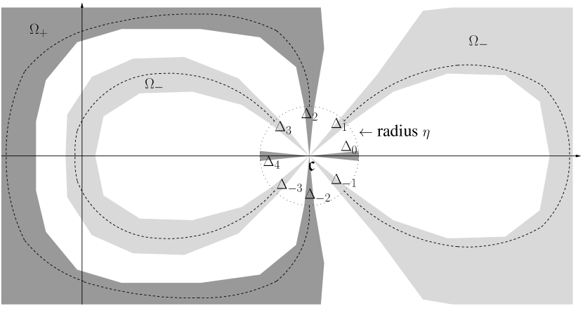
Figure 6: Preparation of the saddle point analysis. The two dotted paths in $\Omega_{-}$ correspond to $\Upsilon^{+}_{res}$ and $\Upsilon^{-}_{res}$ while the dotted path in $\Omega_{+}$ corresponds to $\Xi_{res}$.

The regions $\Delta_{k}$ are shown on Figure 6.

Proof.

Let $\eta>0$ be small enough so that $B(\mathfrak{c},2\eta)\subset\mathbb{C}\setminus\mathcal{K}$. In particular, one can choose a determination of the logarithm such that the map

$$f(z)=-\mathfrak{a}(z-\mathfrak{c})+\log(z)-\gamma\int\log(1-xz)\,\nu({\rm d}x)$$

is well-defined and holomorphic on $B(\mathfrak{c},2\eta)$, and its real part is given by (4.35). Moreover, we have $f^{\prime}(z)=g(z)-\mathfrak{a}$. Since $\mathfrak{a}=g(\mathfrak{c})$ and $g^{\prime}(\mathfrak{c})=g^{\prime\prime}(\mathfrak{c})=0$, a Taylor expansion of $f$ around $\mathfrak{c}$ then yields for every $z\in B(\mathfrak{c},\eta)$,

$$\left|\mathfrak{Re}f(z)-\mathfrak{Re}f(\mathfrak{c})-\frac{1}{4!}g^{(3)}(\mathfrak{c})\mathfrak{Re}(z-\mathfrak{c})^{4}\right| \leqslant\left|f(z)-f(\mathfrak{c})-\frac{1}{4!}g^{(3)}(\mathfrak{c})(z-\mathfrak{c})^{4}\right|$$

$$\leqslant\frac{1}{5!}|z-\mathfrak{c}|^{5}\max_{B(\mathfrak{c},\eta)}|g^{(4)}|.$$

Since $\mathfrak{Re}(z-\mathfrak{c})^{4}=(-1)^{k}r^{4}$ when $z=\mathfrak{c}+re^{ik\pi/4}$, and because $g^{(3)}(\mathfrak{c})>0$, the lemma follows by choosing $\eta$ and then $\theta$ small enough. ∎

Let $\Omega_{2\ell+1}$ be the connected component of $\Omega_{-}$ which contains $\Delta_{2\ell+1}$. Similarly, let $\Omega_{2\ell}$ be the connected component of $\Omega_{+}$ which contains $\Delta_{2\ell}$. We now prove that the following holds true.

Lemma 4.8.

• We have $\Omega_{1}=\Omega_{-1}$, the interior of $\Omega_{1}$ is connected, and for every $0<\alpha<\pi/2$ there exists $R>0$ such that

  $$\left\{z\in\mathbb{C}:\quad|z|>R,\quad-\frac{\pi}{2}+\alpha<\arg(z)<\frac{\pi}{2}-\alpha\right\}\subset\Omega_{1}\ .$$ (4.41)

• We have $\Omega_{2}=\Omega_{-2}$, the interior of $\Omega_{2}$ is connected, and there exists $R>0$ such that

  $$\left\{z\in\mathbb{C}:\quad|z|>R,\quad\frac{\pi}{2}+\alpha<\arg(z)<\frac{3\pi}{2}-\alpha\right\}\subset\Omega_{2}\ .$$ (4.42)

• We have $\Omega_{3}=\Omega_{-3}$, the interior of $\Omega_{3}$ is connected and there exists $\delta>0$ such that $B(0,\delta)\subset\Omega_{3}$.

To prove the lemma, we use the following key properties.

Lemma 4.9.

• If $\Omega_{*}$ is a connected component of $\Omega_{+}$, then $\Omega_{*}$ is open and, if $\Omega_{*}$ is moreover bounded, there exists $x\in\operatorname{Supp}(\nu)$ such that $x^{-1}\in\Omega_{*}$.

• Let $\Omega_{*}$ be a connected component of $\Omega_{-}$ such that $\Omega_{*}\not\subset\mathbb{R}$.

  • If $\Omega_{*}$ is bounded, then $0\in\Omega_{*}$.

  • If $\Omega_{*}$ is bounded, then its interior is connected.

  • If $0\notin\Omega_{*}$, then the interior of $\Omega_{*}$ is connected.

Proof.

See [HHN-preprint, Lemma 4.11]. ∎

Proof of Lemma 4.8.

We first prove (2). Since $\Omega_{2}$ is by definition a connected subset of $\Omega_{+}$, Lemma 4.9–(1) yields that its interior is connected (since $\Omega_{2}$ is open). Next, we show by contradiction that $\Omega_{2}$ is unbounded. If $\Omega_{2}$ is bounded, then Lemma 4.9–(1) shows there exists $x\in\operatorname{Supp}(\nu)$ such that $x^{-1}\in\Omega_{2}$. If $x^{-1}<\mathfrak{c}$ (resp. $x^{-1}>\mathfrak{c}$), then it follows from the symmetry $\mathfrak{Re}f(\overline{z})=\mathfrak{Re}f(z)$ that $\Omega_{2}$ completely surrounds $\Omega_{3}$ (resp. $\Omega_{1}$). As a consequence, $\Omega_{3}\not\subset\mathbb{R}$ (resp. $\Omega_{1}\not\subset\mathbb{R}$) is a bounded connected component of $\Omega_{-}$ which does not contain the origin, and Lemma 4.9–(2a) shows this is impossible. The symmetry $\mathfrak{Re}f(\overline{z})=\mathfrak{Re}f(z)$ moreover provides that $\Omega_{-2}$ is also unbounded, and (2) follows from the inclusion (4.39) and the fact that $\Omega_{+}$ has a unique unbounded connected component, see Lemma 4.6.

We now turn to (1). Since $\Omega_{2}$ is unbounded, then $\Omega_{1}$ does not contain the origin and it follows from Lemma 4.9(2a)-(2c) that $\Omega_{1}$ is unbounded and has a connected interior. Then, (1) follows from symmetry $\mathfrak{Re}f(\overline{z})=\mathfrak{Re}f(z)$, the inclusion (4.38) and the fact that $\Omega_{-}$ has a unique unbounded connected component (cf. Lemma 4.6).

Finally, since $\Omega_{3}$ is bounded as a byproduct of Lemma 4.8–(2), it has a connected interior (Lemma 4.9–(2b)) and contains the origin (Lemma 4.9–(2a)). Moreover, since $\mathfrak{Re}f(z)\to-\infty$ as $z\to 0$, the origin belongs to its interior and, because of the symmetry $\mathfrak{Re}f(\overline{z})=\mathfrak{Re}f(z)$, necessarily $\Omega_{3}=\Omega_{-3}$. Hence (3) is established. ∎

Proof of Proposition 8.

Given any $\rho>0$ small enough, it follows from the convergence of $\mathfrak{c}_{N}$ to $\mathfrak{c}$ that for every $N_{0}$ large enough the points $\mathfrak{c}_{N_{0}}+\rho e^{i\pi/4}$ and $\mathfrak{c}_{N_{0}}+\rho e^{-i\pi/4}$ belong to $\Delta_{1}$ and $\Delta_{-1}$ respectively. Thus both points belong to $\Omega_{1}$ by Lemma 4.8–(1). As a consequence, we can complete the path $\Upsilon^{+}_{o}\cup\Upsilon^{+}_{\times}$ into a closed contour with a path $\Upsilon^{+}_{res}(N_{0})$ lying in the interior of $\Omega_{1}$. Since $\Upsilon^{+}_{res}(N_{0})$ lies in the interior of $\Omega_{1}$, the convergence $\mathfrak{c}_{N}\rightarrow\mathfrak{c}$ moreover yields that we can perform the same construction for all $N\geqslant N_{0}$ with $\Upsilon^{+}_{res}(N)$ in a closed tubular neighbourhood $\mathcal{T}\subset\Omega_{1}$ of $\Upsilon^{+}_{res}(N_{0})$. By Lemma 4.8–(1) again, we can moreover choose $\Upsilon^{+}_{res}(N_{0})$ in a way that it has finite length and only crosses the real axis at a real number lying on the right of $\mathcal{K}$. By construction, this yields that the set $\mathcal{T}$ is compact and that the $\Upsilon^{+}_{res}(N)$’s can be chosen with a uniformly bounded length as long as $N\geqslant N_{0}$. Since $\Omega_{1}\subset\Omega_{-}$ there exists $K>0$ such that $\mathfrak{Re}f(z)\leqslant\mathfrak{Re}f(\mathfrak{c})-3K$ on $\mathcal{T}$. Since moreover $\mathfrak{Re}f_{N}$ uniformly converges to $\mathfrak{Re}f$ on $\mathcal{T}$ and $\mathfrak{Re}f_{N}(\mathfrak{c}_{N})\rightarrow\mathfrak{Re}f(\mathfrak{c})$ according to Lemma 4.5, we can choose $N_{0}$ large enough such that $\mathfrak{Re}f_{N}\leqslant\mathfrak{Re}f+K$ on $\mathcal{T}$ and $\mathfrak{Re}f(\mathfrak{c})\leqslant\mathfrak{Re}f_{N}(\mathfrak{c}_{N})+K$. This finally yields that $\mathfrak{Re}(f_{N}(z)-f_{N}(\mathfrak{c}_{N}))\leqslant-K$ for all $z\in\mathcal{T}$ and proves the existence of a contour $\Upsilon^{+}$ satisfying the requirements of Proposition 8, except for the point (4).

Similarly, the same conclusion for $\Xi$ follows from the same lines but by using $\Omega_{2}$ instead of $\Omega_{1}$ and Lemma 4.8–(2).

We now turn to the contour $\Upsilon^{-}$. Given any $\rho>0$ small enough, for every $N_{0}$ large enough the points $\mathfrak{c}_{N_{0}}-\rho e^{-i\pi/4}$ and $\mathfrak{c}_{N_{0}}-\rho e^{i\pi/4}$ belong to $\Delta_{3}$ and $\Delta_{-3}$ respectively. Thus both points belong to $\Omega_{3}$ by Lemma 4.8–(3), which contains the origin in its interior. As a consequence, we can complete the path $\Upsilon^{-}_{o}\cup\Upsilon^{-}_{\times}$ into a closed contour with a path $\Upsilon^{-}_{res}(N_{0})$ lying in the interior of $\Omega_{3}$, which encircles all the $\lambda_{j}^{-1}$’s smaller than $\mathfrak{c}_{N}$ for every $N$ large enough, since we assumed $\liminf_{N\to\infty}\lambda_{1}>0$. Then, we can follow the same construction as we did for $\Upsilon^{+}$ in order to prove the existence of a contour $\Upsilon^{-}$ satisfying the requirements of Proposition 8, except for the point (4).

Finally, the item (4) of Proposition 8 is clearly satisfied by construction since the sets $\Omega_{-}$ and $\Omega_{+}$ are disjoint, and the proof of the proposition is therefore complete.

∎

Equipped with Proposition 8, we are now in position to establish the remaining estimate towards the proof of Theorem 5.

Proposition 9.

For every $s>0$, the following quantity

$$N^{1/4}\left(\oint_{\Upsilon^{+}\cup\Upsilon^{-}}{\rm d}z\oint_{\Xi}{\rm d}w-\int_{\Upsilon_{*}}{\rm d}z\int_{\Xi_{*}}{\rm d}w\right)\frac{1}{w-z}\,e^{-N^{1/4}x\frac{(z-\mathfrak{c}_{N})}{\sigma_{N}}+N^{1/4}y\frac{(w-\mathfrak{c}_{N})}{\sigma_{N}}+Nf_{N}(z)-Nf_{N}(w)}$$

converges towards zero, uniformly in $x,y\in[-s,s]$, as $N\to\infty$.

Proof.

Let $s>0$ be fixed. This amounts to showing that

$$N^{1/4}\int_{\Upsilon^{+}_{res}\cup\Upsilon^{-}_{res}}{\rm d}z\oint_{\Xi}{\rm d}w\,\frac{1}{w-z}e^{-N^{1/4}x\frac{(z-\mathfrak{c}_{N})}{\sigma_{N}}+N^{1/4}y\frac{(w-\mathfrak{c}_{N})}{\sigma_{N}}+Nf_{N}(z)-Nf_{N}(w)}$$ (4.43)

and

$$N^{1/4}\oint_{\Upsilon}{\rm d}z\int_{\Xi_{res}}{\rm d}w\,\frac{1}{w-z}e^{-N^{1/4}x\frac{(z-\mathfrak{c}_{N})}{\sigma_{N}}+N^{1/4}y\frac{(w-\mathfrak{c}_{N})}{\sigma_{N}}+Nf_{N}(z)-Nf_{N}(w)}$$ (4.44)

converge to zero uniformly in $x,y\in[-s,s]$. First, Lemma 4.2 yields

$$\int_{\Upsilon_{*}}e^{N(\mathfrak{Re}f_{N}(w)-\mathfrak{Re}f_{N}(\mathfrak{c}_{N}))}|{\rm d}z|\leqslant\int_{\Upsilon_{*}}e^{Ng_{N}^{\prime}(\mathfrak{c}_{N})\mathfrak{Re}(z-\mathfrak{c}_{N})^{2}+Ng_{N}^{(3)}(\mathfrak{c}_{N})\mathfrak{Re}(z-\mathfrak{c}_{N})^{4}+N|z-\mathfrak{c}_{N}|^{5}}\ ,$$

and hence, by using the same estimates as in (4.2) an (4.2), we obtain

$$\int_{\Upsilon_{*}}e^{N(\mathfrak{Re}f_{N}(z)-\mathfrak{Re}f_{N}(\mathfrak{c}_{N}))}|{\rm d}z|\leqslant\frac{C}{N^{1/4}}\ .$$ (4.45)

Similarly, using instead (4.25), we get

$$\int_{\Xi_{*}}e^{-N(\mathfrak{Re}f_{N}(w)-\mathfrak{Re}f_{N}(\mathfrak{c}_{N}))}|{\rm d}w|\leqslant\frac{C}{N^{1/4}}\ .$$ (4.46)

Next, Proposition 8 (5-b) yields the existence of $L>0$ independent of $N$ such that, for every $z\in\Upsilon\cup\Xi$, we have $|\mathfrak{Re}(z-\mathfrak{c}_{N})|\leqslant L$. Since

$$e^{Nf_{N}(z)-Nf_{N}(w)}=e^{N(f_{N}(z)-f_{N}(\mathfrak{c}_{N}))}e^{-N(f_{N}(w)-f_{N}(\mathfrak{c}_{N}))},$$

by using moreover Proposition 8 (4) and then Proposition 8 (3-a), we readily obtain

$$N^{1/4}\Bigg{|}\int_{\Upsilon^{+}_{res}\cup\Upsilon^{-}_{res}}{\rm d}z\oint_{\Xi}{\rm d}w\,\frac{1}{w-z}e^{-N^{1/4}x\frac{(z-\mathfrak{c}_{N})}{\sigma_{N}}+N^{1/4}y\frac{(w-\mathfrak{c}_{N})}{\sigma_{N}}+Nf_{N}(z)-Nf_{N}(w)}\Bigg{|}$$

$$\leqslant \qquad\frac{N^{1/4}}{d}\,e^{\frac{2N^{1/4}Ls}{\sigma_{N}}}\int_{\Upsilon^{-}_{res}\cup\Upsilon^{+}_{res}}e^{N(\mathfrak{Re}f_{N}(z)-\mathfrak{Re}f_{N}(\mathfrak{c}_{N}))}|{\rm d}z|\oint_{\Xi}e^{-N(\mathfrak{Re}f_{N}(w)-\mathfrak{Re}f_{N}(\mathfrak{c}_{N}))}|{\rm d}w|$$

$$\leqslant \qquad\frac{N^{1/4}}{d}\,e^{\frac{2N^{1/4}Ls}{\sigma_{N}}-KN}\int_{\Upsilon^{-}_{res}\cup\Upsilon^{+}_{res}}|{\rm d}z|\left(\int_{\Xi_{*}}e^{-N(\mathfrak{Re}f_{N}(w)-\mathfrak{Re}f_{N}(\mathfrak{c}_{N}))}|{\rm d}w|+e^{-NK}\int_{\Xi_{res}}|{\rm d}w|\right).$$

Because of Proposition 8 (5-b) and (4.46), this yields the exponential decay of (4.43) to zero uniform in $x,y\in[-s,s]$. The same holds true for (4.44) by using the same arguments, up to the replacement of Proposition 8 (3-a) by (3-b), and hence the proof of Proposition 9 is complete. ∎

Finally, we can now easily conclude.

4.4 Conclusion

Proof of Theorem 5.

Recalling the integral representation (4.4) for $\widetilde{\rm K}_{N}(x,y)$, we split the contour $\Gamma$ into two pieces $\Gamma^{-}$ and $\Gamma^{+}$, where $\Gamma^{-}$ encircles the $\lambda_{j}^{-1}$’s smaller than $\mathfrak{c}_{N}$, and $\Gamma^{+}$ the $\lambda_{j}^{-1}$’s larger than $\mathfrak{c}_{N}$. Then, we deform $\Theta$ so that it encircles $\Gamma^{-}$. This does not modify the value of the kernel. Indeed, there is no pole at $w=\lambda_{j}^{-1}$ and the residue picked at $w=z$ reads

$$\frac{N^{1/4}}{2i\pi\sigma_{N}}e^{\frac{N^{1/4}}{\sigma_{N}}(y-x)(z-\mathfrak{c}_{N})}$$

and thus vanishes by Cauchy’s theorem since the integrand is analytic.

Now, we can deform by analyticity $\Gamma^{+}$, $\Gamma^{-}$ and $\Theta$ into the respective contours $\Upsilon^{+}$, $\Upsilon^{-}$ and $\Xi$ provided by Proposition 8. Hence, $\widetilde{\rm K}_{N}(x,y)$ equals to

$$\frac{N^{1/4}}{(2i\pi)^{2}\sigma_{N}}\oint_{\Upsilon^{+}\cup\Upsilon^{-}}{\rm d}z\oint_{\Xi}{\rm d}w\,\frac{1}{w-z}\,e^{-N^{1/4}x\frac{(z-\mathfrak{c}_{N})}{\sigma_{N}}+N^{1/4}y\frac{(w-\mathfrak{c}_{N})}{\sigma_{N}}}e^{Nf_{N}(z)-Nf_{N}(w)},$$

and the uniform convergence (4.3) follows for every $s>0$ from Proposition 7 and Proposition 9. The proof of Theorem 5 is therefore complete. ∎

5 Hard edge expansion: Proof of Theorem 6

In this section, we use basic properties of Fredholm determinants and trace class operators. We refer the reader to [book-simon-2005, 17] for comprehensive introductions, see also [HHN-preprint, Section 4.2] for a quick overview. We also use well-known formulas and identities for the Bessel function that can be found in [14].

5.1 Preparation and proof of Theorem 6

Recalling the definition (2.33) of $\sigma_{N}$ and the definition (4.1) of the kernel ${\rm K}_{N}$, we consider here the scaled kernel

$$\widetilde{\rm K}_{N}(x,y)=\frac{1}{N^{2}\sigma_{N}}{\rm K}_{N}\left(\frac{x}{N^{2}\sigma_{N}},\frac{y}{N^{2}\sigma_{N}}\right)\ ,\qquad x,y\in(0,s)\ ,$$ (5.1)

and denote by $\widetilde{\rm K}_{N}$ the associated integral operator acting on $L^{2}(0,s)$. Thus, if $x_{\min}$ is the smallest random eigenvalue of $\mathbf{M}_{N}$ (see (2.32)), we have

$$\mathbb{P}\Big{(}N^{2}\sigma_{N}\,x_{\min}\geqslant s\Big{)}=\det\big{(}I-\widetilde{\rm K}_{N}\big{)}_{L^{2}(0,s)}\ .$$ (5.2)

Recalling the definition (2.29) of the Bessel kernel, [HHN-preprint, Proposition 6.1] states that, for every $s>0$, we have uniformly in $x,y\in(0,s)$ as $N\to\infty$,

$$\widetilde{\rm K}_{N}(x,y)=\left(\frac{x}{y}\right)^{\alpha/2}{\rm K}_{\rm Be}^{(\alpha)}(x,y)+{\mathcal{O}}\left({\frac{1}{N}}\right).$$ (5.3)

Notice that the limiting kernel appearing in the right hand side is exactly (2.30) without the pre-factor $(y/x)^{\alpha/2}$, and hence is bounded on $(0,s)\times(0,s)$. The integral operator associated with this kernel is ${\rm E}{\rm K}_{\rm Be}^{(\alpha)}{\rm E}^{-1}$, where ${\rm E}$ acts on $L^{2}(0,s)$ by ${\rm E}f(x)=x^{\alpha/2}f(x)$. From (5.3), it is easy to derive the convergence

$$\det\big{(}I-\widetilde{\rm K}_{N}\big{)}_{L^{2}(0,s)}\xrightarrow[N\to\infty]{}\det\big{(}I-{\rm K}_{\rm Be}^{(\alpha)}\big{)}_{L^{2}(0,s)}=F_{\alpha}(x)\ .$$ (5.4)

Indeed, (5.3) yields $\det(I-\widetilde{\rm K}_{N})_{L^{2}(0,s)}\to\det(I-{\rm E}{\rm K}_{\rm Be}^{(\alpha)}{\rm E}^{-1})_{L^{2}(0,s)}$ and, for any trace class operators ${\rm A}$,${\rm B}$ on $L^{2}(0,s)$ we have

$$\det(I-{\rm A}{\rm B})_{L^{2}(0,s)}=\det(I-{\rm B}{\rm A})_{L^{2}(0,s)}\ .$$ (5.5)

Thus, (5.4) follows because both the operators ${\rm E}$ and ${\rm K}_{{\rm Be}}^{(\alpha)}{\rm E}^{-1}$ are well-defined on $L^{2}(0,s)$ and trace class when $\alpha\geqslant 0$, and so are the operators ${\rm E}{\rm K}_{\rm Be}^{(\alpha)}$ and ${\rm E}^{-1}$ when $\alpha<0$. See e.g. [HHN-preprint, Section 6] for a proof.

To prove Theorem 6, the first step is to improve (5.3) by making explicit the $1/N$-correction term, and showing the remainder is of order $1/N^{2}$. More precisely, with $\zeta_{N}$ defined as in (2.33), we prove the following kernel expansion.

Proposition 10.

For every $s>0$, we have uniformly in $x,y\in(0,s)$ as $N\to\infty$,

$$\widetilde{\rm K}_{N}(x,y)\\ =\left(\frac{x}{y}\right)^{\alpha/2}\left\{{\rm K}_{\rm Be}^{(\alpha)}(x,y)-\frac{\zeta_{N}}{4\sigma_{N}^{2}N}\Big{(}\alpha J_{\alpha}(\sqrt{x}\,)J_{\alpha}(\sqrt{y}\,)+(x-y){\rm K}_{\rm Be}^{(\alpha)}(x,y)\Big{)}\right\}+{\mathcal{O}}\left({\frac{1}{N^{2}}}\right).$$ (5.6)

The proof of the proposition is deferred to Section 5.2. If ${\rm Q}$ is the integral operator on $L^{2}(0,s)$ with kernel

$${\rm Q}(x,y)=\frac{\zeta_{N}}{4\sigma_{N}^{2}}\Big{(}\alpha J_{\alpha}(\sqrt{x}\,)J_{\alpha}(\sqrt{y}\,)+(x-y){\rm K}_{\rm Be}^{(\alpha)}(x,y)\Big{)},$$ (5.7)

then Proposition 10 yields the operator expansion (for the trace class norm on $L^{2}(0,s)$),

$$\widetilde{\rm K}_{N}={\rm E}\Big{(}{\rm K}_{\rm Be}^{(\alpha)}-\frac{1}{N}{\rm Q}\Big{)}{\rm E}^{-1}+{\mathcal{O}}\left({\frac{1}{N^{2}}}\right).$$ (5.8)

Now, to prove Theorem 6, one just has to plug (5.8) into the Fredholm determinant (5.2), expand it, and identify the $1/N$ order term. For the last step, we need the following lemma, which essentially relies on a formula established by Tracy and Widom.

Lemma 5.1.

We have the identity

$$\mathop{\mathrm{Tr}}\nolimits\big{(}(I-{\rm K}_{\rm Be}^{(\alpha)})^{-1}{\rm Q}\big{)}=-\left(\frac{\alpha\zeta_{N}}{\sigma_{N}^{2}}\right)s\frac{{\rm d}}{{\rm d}s}\log\det\big{(}I-{\rm K}_{{\rm Be}}^{(\alpha)}\big{)}_{L^{2}(0,s)}\ .$$

Proof.

Introduce the trace class operator $\mathrm{M}f(x)=xf(x)$ on $L^{2}(0,s)$, so that one can write

$${\rm Q}=\frac{\zeta_{N}}{4\sigma_{N}^{2}}\Big{(}\alpha J_{\alpha}(\sqrt{\cdot}\,)\otimes J_{\alpha}(\sqrt{\cdot}\,)+[\mathrm{M},{\rm K}_{{\rm Be}}^{(\alpha)}]\Big{)}\ ,$$

where $[{\rm A},{\rm B}]={\rm A}{\rm B}-{\rm B}{\rm A}$. If $\mathrm{R}(x,y)$ is the kernel of the resolvent ${\rm K}_{{\rm Be}}^{(\alpha)}(I-{\rm K}_{{\rm Be}}^{(\alpha)})^{-1}$, then we have

$$\frac{{\rm d}}{{\rm d}s}\log\det\big{(}I-{\rm K}_{{\rm Be}}^{(\alpha)}\big{)}_{L^{2}(0,s)}=-\mathrm{R}(s,s).$$

Equations (2.5) and (2.21) of [tracy-widom-bessel-94] then provide the identity

$$4s\mathrm{R}(s,s)=\big{\langle}J_{\alpha}(\sqrt{\cdot}\,),(I-{\rm K}_{\rm Be}^{(\alpha)})^{-1}J_{\alpha}(\sqrt{\cdot}\,)\big{\rangle}_{L^{2}(0,s)}\ .$$ (5.9)

Since the right hand side of (5.9) equals $\mathop{\mathrm{Tr}}\nolimits\big{(}(I-{\rm K}_{\rm Be}^{(\alpha)})^{-1}J_{\alpha}(\sqrt{\cdot}\,)\otimes J_{\alpha}(\sqrt{\cdot}\,)\big{)}$, the lemma would follow provided that

$$\mathop{\mathrm{Tr}}\nolimits\big{(}(I-{\rm K}_{\rm Be}^{(\alpha)})^{-1}[\mathrm{M},{\rm K}_{{\rm Be}}^{(\alpha)}]\big{)}=0\ ,$$

but this is obvious since $\mathop{\mathrm{Tr}}\nolimits({\rm A}{\rm B})=\mathop{\mathrm{Tr}}\nolimits({\rm B}{\rm A})$ and ${\rm K}_{{\rm Be}}^{(\alpha)}$ commutes with $(I-{\rm K}_{{\rm Be}}^{(\alpha)})^{-1}$. ∎

It is now easy to prove Theorem 6.

Proof of Theorem 6.

The identity (5.2) and the operator expansion (5.8) yield

$$\mathbb{P}\Big{(}N^{2}\sigma_{N}\,x_{\min}\geqslant s\Big{)}=\det\big{(}I-{\rm E}\big{(}{\rm K}_{\rm Be}^{(\alpha)}-\frac{1}{N}{\rm Q}\big{)}{\rm E}^{-1}\big{)}_{L^{2}(0,s)}+{\mathcal{O}}\left({\frac{1}{N^{2}}}\right).$$ (5.10)

By plugging the identity $xJ^{\prime}_{\alpha}(x)=\alpha J_{\alpha}(x)-xJ_{\alpha+1}(x)$ into (2.29), we obtain

$${\rm K}_{{\rm Be}}^{(\alpha)}(x,y)=\frac{\sqrt{x}J_{\alpha+1}(\sqrt{x}\,)J_{\alpha}(\sqrt{y}\,)-\sqrt{y}J_{\alpha+1}(\sqrt{y}\,)J_{\alpha}(\sqrt{x}\,)}{2(x-y)}\ .$$ (5.11)

Combined with the asymptotic behaviour (which follows from the definition (2.28)),

$$J_{\alpha}(\sqrt{x})=\frac{(\operatorname{sign}(\alpha))^{\alpha}}{|\alpha|!}\left(\frac{\sqrt{x}}{2}\right)^{|\alpha|}\big{(}1+O(x)\big{)}\ ,\qquad x\to 0_{+}\ ,$$

it is then easy to check from (5.7) that both ${\rm E}{\rm Q}$ and ${\rm Q}{\rm E}^{-1}$ are trace class and thus, by (5.5),

$$\det\big{(}I-{\rm E}\big{(}{\rm K}_{\rm Be}^{(\alpha)}-\frac{1}{N}{\rm Q}\big{)}{\rm E}^{-1}\big{)}_{L^{2}(0,s)}=\det\big{(}I-{\rm K}_{\rm Be}^{(\alpha)}+\frac{1}{N}{\rm Q}\big{)}_{L^{2}(0,s)}.$$ (5.12)

Finally, using the following expansion of a Fredholm determinant:

$$\det(I-B)=1-\mathop{\mathrm{Tr}}\nolimits(B)+{\mathcal{O}}(\|B\|^{2})\ ,$$

where $B$ is trace class with trace norm $\|B\|<1$, we obtain

$$\det\big{(}I-{\rm K}_{\rm Be}^{(\alpha)}+\frac{1}{N}{\rm Q}\big{)}_{L^{2}(0,s)} =\ \det\big{(}I-{\rm K}_{\rm Be}^{(\alpha)}\big{)}_{L^{2}(0,s)}\det\big{(}I+\frac{1}{N}(I-{\rm K}_{\rm Be}^{(\alpha)})^{-1}{\rm Q}\big{)}_{L^{2}(0,s)}$$

$$=\ \det\big{(}I-{\rm K}_{\rm Be}^{(\alpha)}\big{)}_{L^{2}(0,s)}\Big{(}1+\frac{1}{N}\mathop{\mathrm{Tr}}\nolimits\big{(}(I-{\rm K}_{\rm Be}^{(\alpha)})^{-1}{\rm Q}\big{)}+{\mathcal{O}}\left({N^{-2}}\right)\Big{)}$$

and Theorem 6 follows by combining (5.10), (5.12), (LABEL:bessel_C) together with Lemma 5.1. ∎

We now turn to the proof of the proposition.

5.2 Proof of the kernel expansion

Proof of Proposition 10.

First, by using the representation (5.11) of the Bessel kernel and then the identity $2\alpha J_{\alpha}(x)=xJ_{\alpha+1}(x)+xJ_{\alpha-1}(x)$, we have

$$\alpha J_{\alpha}(\sqrt{x}\,)J_{\alpha}(\sqrt{y}\,)+(x-y){\rm K}_{\rm Be}^{(\alpha)}(x,y)$$

$$=\;\frac{1}{2}\big{(}2\alpha J_{\alpha}(\sqrt{x}\,)J_{\alpha}(\sqrt{y}\,)+\sqrt{x}J_{\alpha+1}(\sqrt{x}\,)J_{\alpha}(\sqrt{y}\,)-\sqrt{y}J_{\alpha}(\sqrt{x}\,)J_{\alpha+1}(\sqrt{y}\,)\big{)}$$

$$=\;\frac{1}{2}\big{(}\sqrt{x}J_{\alpha+1}(\sqrt{x}\,)J_{\alpha}(\sqrt{y}\,)+\sqrt{y}J_{\alpha}(\sqrt{x}\,)J_{\alpha-1}(\sqrt{y}\,)\big{)}.$$

Thus, to prove Proposition 10 is equivalent to show

$$\widetilde{\rm K}_{N}(x,y)=\left(\frac{x}{y}\right)^{\alpha/2}{\rm K}_{\rm Be}^{(\alpha)}(x,y)\\ -\frac{\zeta_{N}}{8\sigma_{N}^{2}N}\left(\frac{x}{y}\right)^{\alpha/2}\Big{(}\sqrt{x}J_{\alpha+1}(\sqrt{x}\,)J_{\alpha}(\sqrt{y}\,)+\sqrt{y}J_{\alpha}(\sqrt{x}\,)J_{\alpha-1}(\sqrt{y}\,)\Big{)}+{\mathcal{O}}\left({\frac{1}{N^{2}}}\right)$$ (5.14)

uniformly in $x,y\in(0,s)$ as $N\to\infty$. To do so, let $0<r<R<\liminf_{N}\lambda_{1}/2$ and introduce the map

$$G_{N}(z)\ =\ \frac{1}{N}\sum_{j=1}^{n}\log\left(\frac{z}{N\sigma_{N}}-\lambda_{j}\right).$$

Recall that Assumption 2 yields $\liminf_{N}\lambda_{1}>0$ and thus one can choose a determination of the logarithm so that $G_{N}$ is well-defined and holomorphic on $\{z\in\mathbb{C}\,,\ |z|<R+1\}$ for every $N$ large enough. In the proof of [HHN-preprint, Proposition 6.1], the following representation has been obtained

$$\widetilde{\rm K}_{N}(x,y)=\frac{1}{(2i\pi)^{2}}\oint_{|z|=r}\frac{{\rm d}z}{z}\oint_{|w|=R}\frac{{\rm d}w}{w}\frac{1}{z-w}\left(\frac{z}{w}\right)^{\alpha}e^{-\frac{x}{z}+\frac{y}{w}-N\left(G_{N}(z)-G_{N}(w)\right)}.$$ (5.15)

Recalling the definitions (2.33) of $\sigma_{N}$ and $\zeta_{N}$, straightforward computations yield

$$G^{\prime}_{N}(z) = \frac{1}{N^{2}\sigma_{N}}\sum_{j=1}^{n}\left(\frac{z}{N\sigma_{N}}-\lambda_{j}\right)^{-1}\ ,\quad G^{\prime}_{N}(0)=-\frac{1}{4N}$$

$$G^{\prime\prime}_{N}(z) = -\frac{1}{N^{3}\sigma_{N}^{2}}\sum_{j=1}^{n}\left(\frac{z}{N\sigma_{N}}-\lambda_{j}\right)^{-2}\ ,\quad G^{\prime\prime}_{N}(0)=-\frac{\zeta_{N}}{8N^{2}\sigma_{N}^{2}}$$

$$G_{N}^{(3)}(z) = \frac{2}{N^{4}\sigma_{N}^{3}}\sum_{j=1}^{n}\left(\frac{z}{N\sigma_{N}}-\lambda_{j}\right)^{-3}\ ,$$

and hence we have the Taylor expansion

$$G_{N}(z)=G_{N}(0)-\frac{z}{4N}-\frac{\zeta_{N}}{16N^{2}\sigma_{N}^{2}}z^{2}+{\mathcal{O}}\left({\frac{1}{N^{3}}}\right),$$ (5.16)

uniformly valid for $|z|\leqslant R+1$. Plugging this Taylor expansion into (5.15) and recalling the contour integral representation (2.30) of the Bessel kernel, we readily obtain as $N\to\infty$,

$$\widetilde{\rm K}_{N}(x,y) = \frac{1}{(2i\pi)^{2}}\oint_{|z|=r}\frac{{\rm d}z}{z}\oint_{|w|=R}\frac{{\rm d}w}{w}\frac{1}{z-w}\left(\frac{z}{w}\right)^{\alpha}e^{-\frac{x}{z}+\frac{y}{w}+\frac{z}{4}-\frac{w}{4}}$$ (5.17)

$$\qquad\times\exp\left(\frac{\zeta_{N}}{16N\sigma_{N}^{2}}(z^{2}-w^{2})+{\mathcal{O}}\left(\frac{1}{N^{2}}\right)\right)$$

$$= \frac{1}{(2i\pi)^{2}}\oint_{|z|=r}\frac{{\rm d}z}{z}\oint_{|w|=R}\frac{{\rm d}w}{w}\frac{1}{z-w}\left(\frac{z}{w}\right)^{\alpha}e^{-\frac{x}{z}+\frac{y}{w}+\frac{z}{4}-\frac{w}{4}}$$

$$\qquad\times\left(1+\frac{\zeta_{N}}{16N\sigma_{N}^{2}}(z^{2}-w^{2})+{\mathcal{O}}\left(\frac{1}{N^{2}}\right)\right)$$

$$= \left(\frac{x}{y}\right)^{\alpha/2}{\rm K}_{{\rm Be}}^{(\alpha)}(x,y)$$

$$\qquad+\left(\frac{\zeta_{N}}{16N\sigma_{N}^{2}}\right)\frac{1}{(2i\pi)^{2}}\oint_{|z|=r}\frac{{\rm d}z}{z}\oint_{|w|=R}\frac{{\rm d}w}{w}\,(z+w)\left(\frac{z}{w}\right)^{\alpha}e^{-\frac{x}{z}+\frac{y}{w}+\frac{z}{4}-\frac{w}{4}}$$

$$\qquad\qquad+\;{\mathcal{O}}\left({\frac{1}{N^{2}}}\right)$$

uniformly for $x,y\in(0,s)$. In the light of (5.14), we are left to show that

$$\frac{1}{(2i\pi)^{2}}\oint_{|z|=r}\frac{{\rm d}z}{z}\oint_{|w|=R}\frac{{\rm d}w}{w}\,(z+w)\left(\frac{z}{w}\right)^{\alpha}e^{-\frac{x}{z}+\frac{y}{w}+\frac{z}{4}-\frac{w}{4}}\\ =-2\left(\frac{x}{y}\right)^{\alpha/2}\Big{(}\sqrt{x}J_{\alpha+1}(\sqrt{x}\,)J_{\alpha}(\sqrt{y}\,)+\sqrt{y}J_{\alpha}(\sqrt{x}\,)J_{\alpha-1}(\sqrt{y}\,)\Big{)}$$ (5.18)

in order to complete the proof of the proposition. But this easily follows from the contour integral representations of the Bessel function,

$$J_{\alpha}(\sqrt{x}\,)=\frac{(-1)^{\alpha}}{2i\pi(2\sqrt{x}\,)^{\alpha}}\oint_{|z|=r}z^{\alpha}e^{-\frac{x}{z}+\frac{z}{4}}\frac{{\rm d}z}{z}\ ,\quad J_{\alpha}(\sqrt{y}\,)=(-1)^{\alpha}\frac{(2\sqrt{y}\,)^{\alpha}}{2i\pi}\oint_{|w|=R}\frac{e^{\frac{y}{w}-\frac{w}{4}}}{w^{\alpha}}\frac{{\rm d}w}{w}\ ,$$ (5.19)

see for instance [HHN-preprint, Eq. (164) and (165)] and perform the respective changes of variables $z\mapsto-z^{-1}$ and $w\mapsto-w^{-1}$. The proof of the proposition is therefore complete.

∎

Remark 5.2.

By extending the Taylor expansion (5.16) to higher order terms, the computation (5.17) easily yields the kernel expansion as $N\to\infty$, uniform in $x,y\in(0,s)$,

$$\widetilde{\rm K}_{N}(x,y)=\left(\frac{x}{y}\right)^{\alpha/2}\Big{\{}{\rm K}_{{\rm Be}}^{(\alpha)}(x,y)+\sum_{\ell=1}^{L}\frac{1}{N^{\ell}}{\rm Q}_{N}^{(\ell)}(x,y)\Big{\}}+{\mathcal{O}}\left({\frac{1}{N^{L+1}}}\right)$$

for every $L\geqslant 1$. The kernels ${\rm Q}_{N}^{(\ell)}(x,y)$ can be expressed in terms of sums of Bessel functions (by using (5.19)). By plugging this formula into the Fredholm determinant (5.2), and expanding it, this yields an asymptotic expansion of the form (2.35), although we are not able to provide a simple representation for the coefficients $C_{N,\ell}^{(\alpha)}(s)$ when $\ell\geqslant 2$. It would be interesting to identify these coefficients in terms of $F_{\alpha}(s)$ if it is possible.

References

- [1]
- [2] M. Adler, M. Cafasso, P. van Moerbeke, Nonlinear PDEs for gap probabilities in random matrices and KP theory, Physica D: Nonlinear Phenomena 241 (2012), 2265–2284.
- [3] G. Anderson, A. Guionnet, O. Zeitouni, An Introduction to Random Matrices, Cambridge University Press, 2009.
- [4] J. Baik, G. Ben Arous, S. Péché, Phase transition of the largest eigenvalue for nonnull complex sample covariance matrices, Ann. Probab. 33 (2005), 1643–1697.
- [5] M. Bertola, M. Cafasso, The transition between the gap probabilities from the Pearcey to the Airy Process; a Riemann–Hilbert approach, Int. Math. Res. Not. 2012 no. 7, 1519–1568.
- [6] P. M. Bleher, A.B.J. Kuijlaars, Large n limit of Gaussian random matrices with external source, part III: double scaling limit, Comm. Math. Phys. 270 (2007), 481–517.
- [7] F. Bornemann, A note on the expansion of the smallest eigenvalue distribution of the LUE at the hard edge, preprint 3p (2015), arXiv:1504.00235.
- [8] E. Brézin, S. Hikami, Universal singularity at the closure of a gap in a random matrix theory, Phys. Rev. E 57 (1998), 4140–4149.
- [9] E. Brézin, S. Hikami, Level spacing of random matrices in an external source, Phys. Rev. E 58 (1998), 7176–7185.
- [10] M. Capitaine, S. Péché, Fluctuations at the edge of the spectrum of the full rank deformed GUE, preprint 44p (2014), arXiv:1402.2262.
- [11] E. Duse, A. Metcalfe, Asymptotic Geometry of Discrete Interlaced Patterns: Part I, preprint 57p (2015), arXiv:1412.6653.
- [12] E. Duse, A. Metcalfe, Universal edge fluctuations of discrete interlaced particle systems. In preparation.
- [13] A. Edelman, A. Guionnet, S. Péché, Beyond universality in random matrix theory, preprint 42p (2014), arXiv:1405.7590.
- [14] A. Erdélyi, W. Magnus, F. Oberhettinger, F. G. Tricomi, Higher Transcendental Functions, Vol. 2 (McGraw-Hill, New York, 1953).
- [15] N. El Karoui, Tracy-Widom limit for the largest eigenvalue of a large class of complex sample covariance matrices, Ann. Probab. 35 (2007), 663–714.
- [16] P. J. Forrester, The spectrum edge of random matrix ensembles, Nucl. Phys. B 402 (1993), 709–728.
- [17] I. Gohberg, S. Goldberg, N. Krupnik, Traces and determinants of linear operators, \btxvolumelong \btxvolumefont116 \btxofserieslong \btxtitlefontOperator Theory: Advances and Applications. \btxpublisherfontBirkhäuser Verlag, Basel, 2000