Local observability of state variables and parameters in nonlinear modeling quantified by delay reconstruction

Abstract

Features of the Jacobian matrix of the delay coordinates map are exploited for quantifying the robustness and reliability of state and parameter estimations for a given dynamical model using an observed time series. Relevant concepts of this approach are introduced and illustrated for discrete and continuous time systems employing a filtered Hénon map and a Rössler system.

For many physical processes dynamical models (differential equations or iterated maps) are available but often not all of their variables and parameters are known or can be (easily) measured. In meteorology, for example, sophisticated large scale models exist, which have to be continuously adapted to the true temporal changes of temperatures, wind speed, humidity, and other relevant physical quantities. To obtain a model that “follows” reality, measured data have to be repeatedly incorporated into the model. In geosciences this procedure is called data assimilation, but the task to track state variables and system parameters by means of estimation methods occurs also in other fields of physics and applications. However, not all observables provide the information required to estimate a particular unknown quantity. In this article, we consider this problem of observability in the context of chaotic dynamics where sensitive dependance on initial conditions complicates any estimation method. A quantitative characterization of local observability employing delay coordinates is used to answer the question where in state and parameter space estimation of a particular state variable or parameter is feasible and where not.

I Introduction

180(18,262) Copyright 2014 American Institute of Physics. This article may be downloaded for personal use only. Any other use requires prior permission of the author and the American Institute of Physics. The following article appeared in U. Parlitz et al., Chaos 24, 024411 (2014) and may be found at http://dx.doi.org/10.1063/1.4884344. To describe and forecast dynamical processes in physics and many other fields of science mathematical models are used, like, for example, ordinary differential equations (ODEs), partial differential equations (PDEs), or iterated maps. Some of these models are derived from first principles while others are the result of a general black-box modeling approach (e.g., based on neural networks). These models typically contain two kinds of variables and parameters: those that can be directly measured or are known beforehand (e.g., fundamental physical constants) and others whose values are unknown and very difficult to accessVTK04 ; RBKT10 . To estimate the latter estimation methods have been devised that aim at extracting the required information from the dynamics, here represented by the model equations and the experimentally observed dynamical evolution of the underlying process. Different approaches for solving this dynamical estimation problem have been devised in the past, including (nonlinear) observer or synchronization schemes PJK96 ; NM97 ; HLN01 ; GB08 ; ACJ08 ; SO09 ; SRL09 ; K05 ; FMG05 ; CK07 ; Amritkar09 , particle filters L10 , a path integral formalism A09 ; QA10 , or optimization based algorithms CGA08 ; B10 ; SBP11 .

Before applying such an estimation method one may ask whether the available time series (observable) actually contains the required information to estimate a particular unknown value. In control theory this is called observability problem and it can for linear systems of ODEs be analyzed and answered by means of the so-called observability matrix Sontag ; NS90 . Using derivative coordinates this approach can be generalized for nonlinear continuous systems HK77 ; Sontag ; N82 . For state estimation of chaotic systems Letellier, Aguirre and Maquet LAM05 ; AL05 ; LAM06 ; LA09 ; FBL12 considered continuous dynamical systems

$$\dot{\mathbf{x}}=\mathbf{f}(\mathbf{x})$$ (1)

that generate some observed signal $s(t)=h(\mathbf{x}(t))\in\mathbb{R}$ where $\mathbf{x}\in{\cal{U}}\subset{\mathbb{R}}^{M}$ is the state of the system, ${\cal{U}}$ is a smooth submanifold of $\mathbb{R}^{M}$, and $h:\mathbb{R}^{M}\to\mathbb{R}$ denotes a measurement or observation function. Consider now $D$-dimensional derivative coordinates Aeyels ; Takens ; SYC91 ; KS97 ; book_HDIA of the observed signal $s(t)$

$$\mathbf{y}=\left(s,\dot{s},\ddot{s},\ldots,s^{(D-1)}\right)=F(\mathbf{x})\in\mathbb{R}^{D}$$ (2)

where $s^{(k)}$ stands for the $k$-th temporal derivative of $s(t)$, $D$ is the reconstruction dimension, and $F$ is called derivative coordinates map SYC91 . If this map is (at least locally) invertible, then we can uniquely determine the full state vector $\mathbf{x}(t)\in{\cal{U}}$ from the signal $s(t)$ and its higher derivatives LAF09 . Furthermore, small perturbations in $\mathbf{y}$ should correspond to small perturbations in $\mathbf{x}$ and vice versa. Therefore, we want the map $F:{\cal{U}}\to F({\cal{U}})\subset\mathbb{R}^{D}$ to be an immersion, i.e. a smooth map whose derivative map is one-to-one at every point of ${\cal{U}}$, or equivalently, whose Jacobian matrix $DF(\mathbf{x})$ has full rank on the tangent space (here $\mbox{rank}(DF(\mathbf{x}))=M\ \forall\mathbf{x}\in{\cal{U}}$). This does not imply that the map $F$ itself is one-to-one ($F(\mathbf{x})=F(\mathbf{z})\Rightarrow\mathbf{x}=\mathbf{z}$), since the derivative coordinates (2) may provide states $\mathbf{y}\in\mathbb{R}^{D}$ with two (or more) pre-images separated by a finite distance. Therefore, the observability analysis presented in the following is local, only, because it is based on analyzing (the rank) of the Jacobian matrix $DF$. The (global) one-to-one property of the map $F$ is not checked (what would be necessary, and for compact U also sufficient, to show that $F$ is an embedding SYC91 ).

The $D\times M$ Jacobian matrix $DF(\mathbf{x})$ can be computed by means of the vector field given in Eq. (1). In fact, for linear ODEs the Jacobian matrix $DF(\mathbf{x})$ conforms with the observability matrix known from (linear) control theory AL05 . To estimate the rank of $DF(\mathbf{x})$ Letellier, Aguirre, and Maquet LAM05 ; AL05 suggest to compute the eigenvalues $\mu_{k}\geq 0$ of the $M\times M$ - matrix

$$A(\mathbf{x})=DF^{tr}(\mathbf{x})\cdot DF(\mathbf{x}).$$ (3)

Nonzero eigenvalues indicate full rank of $DF(\mathbf{x})$ and thus local invertibility of $F$ at $\mathbf{x}$. To quantify the (local) invertibility of $F(\mathbf{x})$ and thus the (local) observability of the full state $\mathbf{x}$ Aguirre, Letellier, and Maquet LAM05 ; AL05 introduced the observability index

$$\delta(\mathbf{x})=\frac{\mu_{min}(A)}{\mu_{max}(A)}$$ (4)

where $\mu_{min}(A)$ and $\mu_{max}(A)$ denote the smallest and the largest eigenvalue of the matrix $A$, respectively. Time averaging (along the available trajectory for $0\leq t\leq T$) yields

$$\bar{\delta}=\frac{1}{T}\int_{0}^{T}\delta(\mathbf{x}(t))dt.$$ (5)

Instead of derivative coordinates we consider in the following delay coordinates Aeyels ; Takens ; SYC91 ; KS97 ; book_HDIA . Furthermore, we extend the observability analysis to parameter estimation and compute a specific measure of uncertainty PSBL for each state variable or parameter to be estimated. Last not least, we are not only interested in quantifying the average observability (like $\bar{\delta}$ in Eq. (5)) but also in local variations that can be exploited during the state and parameter estimation process.

II Delay coordinates and observability

To motivate the concepts to be presented in the following we shall first consider a discrete time system (iterated map) where all model parameters are known and only state variables have to be estimated from the observed time series.

II.1 Estimating state variables of a filtered Hénon map

For an $M$ dimensional discrete system

$$\mathbf{x}(n+1)=\mathbf{g}(\mathbf{x}(n))$$ (6)

which generates the times series $\{s(n)\}$ with $s(n)=h(\mathbf{x}(n))$ where $n=1,...,N$ we can construct $D$ dimensional delay coordinates Aeyels ; Takens ; SYC91 ; KS97 ; book_HDIA with reconstructed states

$$\mathbf{y}(n) = \left(s(n),s(n+1),....,s(n+D-1)\right)$$

$$= G_{+}(\mathbf{x}(n))\in\mathbb{R}^{D}.$$

Again we assume that all states of interest $\mathbf{x}$ lie within a smooth manifold ${\cal{U}}\subset\mathbb{R}^{M}$. Here we consider delay coordinates forward in time. The function $G_{+}$ is therefore called forward delay coordinates map $G_{+}:{\cal{U}}\to G_{+}({\cal{U}})\subset\mathbb{R}^{D}$. It is also possible to use delay coordinates backward in time, or mixed forward and backward, and we shall address this issue in Sec. II.2.

As already discussed with derivative coordinates in the previous section a state $\mathbf{x}=(x_{1},\ldots,x_{M})$ is locally observable from the time series $\{s(n)\}$ if $G$ is an immersion, i.e. if the Jacobian matrix $DG(\mathbf{x})$ has maximal (full) rank $M$ at $\mathbf{x}$. The corresponding $D\times M$ Jacobian matrix $DG(\mathbf{x})$ can be computed using the iterated map Eq. (6). If the Jacobian matrix $DG(\mathbf{x})$ has maximal rank $M$ (assuming $M\leq D$) then $G$ is locally invertible (on $G({\cal{U}})$). “Local” means that still a delay vector $\mathbf{y}$ could possess different pre images (separated by a finite distance).

To motivate and illustrate this analysis we consider the Hénon map

$$x_{1}(n+1) = 1-ax_{1}^{2}(n)+bx_{2}(n)$$ (8)

$$x_{2}(n+1) = x_{1}(n)$$ (9)

with parameters $a=1.4$ and $b=0.3$. In the following we shall assume that the dynamics of this system is observed via a filtered signal $s(n)$ provided by an FIR-filter

$$s(n) = x_{1}(n)+cx_{1}(n-1)$$ (10)

$$= x_{1}(n)+cx_{2}(n)=h(\mathbf{x}(n))$$

with filter parameter $c$.

For two dimensional delay coordinates the delay coordinates map reads

$$G({\bf x}(n)) = (s(n),s(n+1))$$

$$= (x_{1}(n)+cx_{2}(n),$$

$$\ \ \ \ \ \ \ \ 1-ax_{1}^{2}(n)+bx_{2}(n)+cx_{1}(n))$$

or

$$G(\mathbf{x})=(x_{1}+cx_{2},1-ax_{1}^{2}+bx_{2}+cx_{1}).$$ (11)

The Jacobian matrix of the map $G$ is given by:

$$DG(\mathbf{x})=\left(\begin{array}[]{ccc}1&c\\ -2ax_{1}+c&b\end{array}\right)$$ (12)

and its determinant

$$\det(DG(\mathbf{x}))=2acx_{1}+b-c^{2}$$ (13)

vanishes for all states $\mathbf{x}=(x_{1},x_{2})$ on the singular line

$$x_{1}^{s}=\frac{c^{2}-b}{2ac}.$$ (14)

For $c\to 0$ the FIR-filter is (asymptotically) deactivated and the critical line disappears ($c\to 0\Rightarrow x_{1}^{s}\to-\infty$). For $0.0867<c<3.66$, however, the critical line crosses the chaotic attractor as shown for $c=0.5$ in Fig. 1a.

Figure 1: (Color online) (a), (b) Hénon attractor and singular axes $\frac{1}{\sigma_{1}}\mathbf{V}^{(1)}$ (short, blue) and $\frac{1}{\sigma_{2}}\mathbf{V^{(2)}}$ (longer, red) for filter parameter $c=0.5$. (c), (d) Delay coordinates for $c=0.5$ ($x_{1}^{s}=-0.0357$) and $c=0.08$ ($x_{1}^{s}=-1.311$).

II.2 Forward, backward, and mixed delay coordinates

Instead of using state space reconstruction based on forward delay coordinates (II.1) one could also use backward delay coordinates

$$\mathbf{y}(n) = \left(s(n),s(n-1),\ldots,s(n-D+1)\right)$$

$$= G_{-}(\mathbf{x}(n))\in\mathbb{R}^{D}$$

or more general, a combination of forward and backward components

$$\mathbf{y}(n) = \left(s(n-D_{-}),\ldots s(n-1),s(n),s(n+1),\right.$$

$$\left.\ldots,s(n+D_{+})\right)$$

$$= G_{\pm}(\mathbf{x}(n);D_{-},D_{+})\in\mathbb{R}^{D}$$

called mixed delay coordinates in the following, with reconstruction dimension $D=1+D_{-}+D_{+}$. To obtain the backward components $s(n-k)=h(({\mathbf{x}}(n-k))$ the inverse map ${\mathbf{x}}(n-1)={\mathbf{g}}^{-1}({\mathbf{x}}(n))$ and its Jacobian matrix are required (here we assume that the dynamics is time invertible). For discrete time systems (like the Hénon example) the underlying map (6) has to be inverted and for continuous time systems the inverse of the flow can in principle be computed by integrating the system ODEs (1) backward in time. In both cases, however, problems may occur in practice, because an explicit form of the inverse map may not exist and backward integration of dissipative systems results in diverging solutions and numerical instabilities (for longer integration times). Despite these difficulties inclusion of backward components turns out to be beneficial for the estimation task as will be demonstrated in the following for the Hénon examples and the Rössler system.

II.3 Noisy observations and uncertainty

At states $(x_{1},x_{2})$ with $x_{1}\neq x_{1}^{c}$ the delay coordinates map $G$ is in principle invertible, but the inverse can be very susceptible to perturbations in $\mathbf{y}$ like measurement noise. To quantify the robustness and the sensitivity of the inverse with respect to noise we consider the singular value decomposition of the Jacobian matrix $DG$ of the delay coordinates map

$$DG=U\cdot S\cdot V^{tr}$$ (17)

where $S=\rm{diag}(\sigma_{1},\ldots,\sigma_{M})$ is an $M\times M$ diagonal matrix containing the singular values $\sigma_{1}\geq\sigma_{2}\geq\ldots\geq\sigma_{M}\geq 0$ and $U=(\mathbf{u}^{(1)},\ldots,\mathbf{u}^{(M)})$ and $V=(\mathbf{v}^{(1)},\ldots,\mathbf{v}^{(M)})$ are orthogonal matrices, represented by the column vectors $\mathbf{u}^{(i)}\in\mathbb{R}^{D}$ and $\mathbf{v}^{(i)}\in\mathbb{R}^{M}$, respectively. $V^{tr}$ is the transposed of $V$ coinciding with the inverse $V^{-1}=V^{tr}$. Analogously, $U^{tr}=U^{-1}$ and the inverse Jacobian matrix reads

$$DG^{-1}=V\cdot S^{-1}\cdot U^{tr}$$ (18)

where $S^{-1}=\rm{diag}(1/\sigma_{1},\ldots,1/\sigma_{M})$. Multiplying by $U$ from the right we obtain $DG^{-1}U=V\cdot S^{-1}$ or

$$DG^{-1}{\mathbf{u}}^{(m)}=\frac{1}{\sigma_{m}}{\mathbf{v}}^{(m)}\ \ \ \ \ (m=1,\ldots,M).$$ (19)

This transformation is illustrated in Fig. 2 and it describes how small perturbations of $\mathbf{y}$ in delay reconstruction space result in deviations from $\mathbf{x}$ in the original state space. Most relevant for the observability of the (original) state $\mathbf{x}$ is the length of the longest principal axis of the ellipsoid given by the inverse of the smallest singular value $\sigma_{M}$ (see Fig. 2). Small singular values correspond to directions in state space where it is difficult (or even impossible) to locate the true state $\mathbf{x}$ given a finite precision of the reconstructed state $\mathbf{y}$. For the filtered Hénon map we find that the closer the state $\mathbf{x}$ is to the critical line given by $x_{1}^{s}$ (14) the more severe is this uncertainty. This is illustrated in Fig. 1a,b where at some points $\mathbf{x}$ the ellipses spanned by the column vectors of the matrix $V\cdot S^{-1}$ are plotted. Figure 3 shows (color coded) the logarithm of the ratio smallest singular value $\sigma_{min}=\sigma_{M}$ (here: $M=2$) divided by the largest singular value $\sigma_{max}=\sigma_{1}$ vs. state variables $x_{1}$ and $x_{2}$ in a range of coordinates containing the chaotic Hénon attractor. In Fig. 3a $D=2$ dimensional forward delay (II.1) is considered where at $x_{1}^{s}$ the smallest singular value $\sigma_{min}=\sigma_{M}=\sigma_{2}$ vanishes indicating the singularity (14) illustrated in Fig. 1a,b. If the reconstruction dimension $D$ is increased from $D=2$ to $D=3$ the singularity disappears as can be seen in Fig. 3b showing the ratio $\sigma_{min}/\sigma_{max}$ (color coded) for $D=3$ dimensional forward delay coordinates. For comparison, Figs. 3c,d show results obtained with mixed delay coordinates (II.2) and backward delay coordinates (II.2), respectively. The white areas in Fig. 3d correspond to ratios $\sigma_{min}/\sigma_{max}<0.01$ indicating poor observability (due to fast divergence of backward iterates of the Hénon map). Further increase of the reconstruction dimension ($D=4$ or $D=5$) results in even larger values of $\sigma_{min}/\sigma_{max}$ (not shown here).

To assess the observability on the Hénon attractor we computed histograms of ratios $\sigma_{min}/\sigma_{max}$ at $10^{6}$ points. Figure 4 shows these histograms for the same coordinates used to generate the corresponding diagrams in Fig. 3. The best results (large ratios) provide mixed delay coordinates (Fig. 4c). We speculate that this is due to the fact that forward and backward components cover different directions in state space (similar to Lyapunov vectors corresponding to positive and negative Lyapunov exponents).

Figure 2: (Color online) The inverse Jacobian $DG^{-1}(\mathbf{y})$ maps perturbations of $\mathbf{y}$ in delay reconstruction space to deviations from the state $\mathbf{x}$ whose magnitudes depend on the direction of the perturbation as described by Eq. (19).

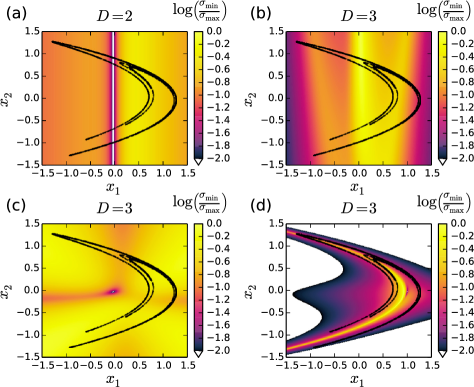
Figure 3: (Color online) Local observability of the filtered Hénon map (8)-(10). Logarithm of the (color coded) ratio of the smallest singular value $\sigma_{min}=\sigma_{M}$ ($M=2$) divided by largest singular value $\sigma_{max}=\sigma_{1}$ vs. coordinates $x_{1}$ and $x_{2}$ for $c=0.5$. (a) $D=2$ dimensional forward delay coordinates (II.1), (b) $D=3$ dimensional forward delay coordinates (II.1), (c) $D=3$ dimensional mixed delay coordinates (II.2) ($D_{-}=1=D_{+}$), and (d) $D=3$ dimensional backward delay coordinates (II.2).

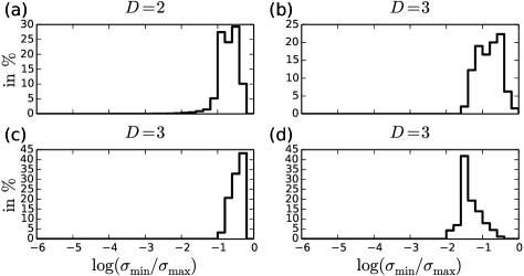
Figure 4: (Histograms of rations $\sigma_{min}/\sigma_{max}$ computed at $10^{6}$ points of the Hénon attractor with: (a) $D=2$ dimensional forward delay coordinates (II.1), (b) $D=3$ dimensional forward delay coordinates (II.1), (c) $D=3$ dimensional mixed delay coordinates (II.2) ($D_{-}=1=D_{+}$), and (d) $D=3$ dimensional backward delay coordinates (II.2). Compare corresponding diagrams in Fig. 3.

If the perturbations of the reconstructed state $\mathbf{y}$ are due to normally distributed measurement noise they can be described by a symmetric Gaussian distribution centered at $\mathbf{y}$

$$Q(\mathbf{\tilde{y}})=\frac{\exp\left[-\frac{1}{2}({\mathbf{\tilde{y}}}-{\mathbf{y}})^{tr}\Sigma_{y}^{-1}({\mathbf{\tilde{y}}}-{\mathbf{y}})\right]}{\sqrt{(2\pi)^{D}\det(\Sigma_{y})}}$$ (20)

where $\Sigma_{y}={\rm{diag}}(\rho^{2},\ldots,\rho^{2})=\rho^{2}I_{D}$ denotes the $D\times D$ covariance matrix ($I_{D}$ stands for the $D$-dimensional unit matrix) and the standard deviation $\rho$ quantifies the noise amplitude. For (infinitesimally) small perturbations $\mathbf{\Delta y}=\mathbf{\tilde{y}}-\mathbf{y}$ this distribution is mapped by the (pseudo) inverse of the delay coordinates map to the (non-symmetrical) distribution

$$P(\mathbf{\tilde{x}})=\frac{\exp\left[-\frac{1}{2}(\mathbf{\tilde{x}}-\mathbf{x})^{tr}\Sigma_{x}^{-1}(\mathbf{\tilde{x}}-\mathbf{x})\right]}{\sqrt{(2\pi)^{M}\det(\Sigma_{x})}}$$ (21)

centered at $\mathbf{x}$ with the inverse covariance matrix

$$\Sigma_{x}^{-1} = DG^{tr}\cdot\Sigma_{y}^{-1}\cdot DG=\frac{1}{\rho^{2}}DG^{tr}\cdot DG$$ (22)

$$= \frac{1}{\rho^{2}}V\cdot S^{2}\cdot V^{tr}.$$ (23)

The marginal distribution $P_{j}$ of a given state variable $\tilde{x}_{j}$ centered at $x_{j}$ is given by

$$P_{j}(\tilde{x}_{j})=\frac{1}{\rho_{j}\sqrt{2\pi}}\exp\left[-\frac{(\tilde{x}_{j}-x_{j})^{2}}{2\rho_{j}^{2}}\right]$$ (24)

where the standard deviation $\rho_{j}$ is given by the square root of the diagonal elements of the covariance matrix

$$\rho_{j}=\sqrt{\Sigma_{x,jj}}.$$ (25)

Using Eq. (22) the standard deviation of the marginal distribution $P_{j}$ can be written

$$\rho_{j}=\rho\sqrt{\left[DG^{tr}\cdot DG\right]^{-1}_{jj}}=\rho\sqrt{\left[V\cdot S^{-2}\cdot V^{tr}\right]_{jj}}$$ (26)

and we consider in the following the factor

$$\nu_{j}=\sqrt{\left[DG^{tr}\cdot DG\right]^{-1}_{jj}}=\sqrt{\left[V\cdot S^{-2}\cdot V^{tr}\right]_{jj}}$$ (27)

as our measure of uncertainty when estimating $x_{j}$, because it quantitatively describes how the initial standard deviation $\rho$ is amplified when estimating variable $x_{j}$ PSBL .

Figure 5 shows the uncertainties $\nu_{1}$ and $\nu_{2}$ vs. $(x_{1},x_{2})$ for different $D=3$ dimensional delay coordinates. In Fig. 4a,b results obtained with $D=3$ dimensional forward delay coordinates (II.1) are given. Large uncertainties occur mainly in a vertical stripe located near the singularity at $x_{1}^{s}$ (Eq. (14)) occurring for $D=2$. Figures 5c,d,e,f show uncertainties of $x_{1}$ and $x_{2}$ obtained with mixed delay coordinates ((c),(d)) and backward delay coordinates ((e), (f)). For mixed delay coordinates (Fig. 5c,d) areas with very high uncertainties occur near the origin, but along the attractor $\nu_{1}$ and $\nu_{2}$ take only relatively low values. This is also confirmed by the $\nu$-histograms on the attractor given in Fig. 6 for the same delay coordinates as used in Fig. 4. Again, the mixed delay coordinates turns out to be superior to the purely forward or backward coordinates. Furthermore, the dependance of the range of uncertainty values on the type of coordinates is different for different variables. While the uncertainty $\nu_{1}$ of $x_{1}$ increases when changing from forward to backward delay coordinates (Figs. 6a,e), the uncertainty of $x_{2}$ exhibits the opposite trend (Figs. 6b,f).

Figure 5: (Color online) Uncertainty (27) of the variables $x_{1}$ and $x_{2}$ of the Hénon map for $c=0.5$ and different $D=3$ dimensional delay coordinates. (a), (b) forward coordinates (II.1), (c), (d) mixed coordinates (II.2), and (e), (f) backward coordinates (II.2).

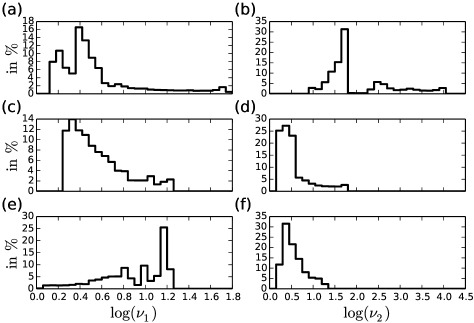
Figure 6: Histograms of uncertainties (27) of $x_{1}$ and $x_{2}$ on the Hénon attractor (computed at $10^{6}$ points) for $D=3$ and $c=0.5$ with (a), (b) forward, (c), (d) mixed, and (e), (f) backward delay coordinates (comp. Fig. 4).

II.4 State and parameter estimation

Until now only the state variables $x_{1}$ and $x_{2}$ are considered as unknowns to be estimated and the parameters $a$ and $b$ of the Hénon map and $c$ of the FIR filter are assumed to be known. We shall now consider the general case including unknown parameters $\mathbf{p}=(p_{1},\ldots,p_{P})\in\mathbb{R}^{P}$ of the dynamical system and unknown parameters $\mathbf{q}=(q_{1},\ldots,q_{Q})\in\mathbb{R}^{Q}$ of the measurement function $h(\mathbf{x},\mathbf{q})$. Let the dynamical model be a $M$-dimensional discrete

$$\mathbf{x}(n+1)={\mathbf{g}}(\mathbf{x}(n),\mathbf{p})$$ (28)

or a continuous

$$\dot{\mathbf{x}}={\mathbf{f}}({\mathbf{x}},\mathbf{p})$$ (29)

dynamical system generating a flow

$$\phi^{t}:\mathbb{R}^{M}\rightarrow\mathbb{R}^{M}$$ (30)

with discrete $t=n\in\mathbb{Z}$ or continuous $t\in\mathbb{R}$ time. Furthermore, let’s assume that a time series $\{s(n)\}$ of length $N$ is given observed via the measurement function

$$s(t)=h(\phi^{t}(\mathbf{x},\mathbf{p}),\mathbf{q})$$ (31)

from a trajectory starting at $\mathbf{x}$.

This provides the $D$-dimensional delay coordinates

$$\mathbf{y} = \left(s(-D_{-}\tau_{-}),\ldots,s(-\tau_{-}),s(0),s(\tau_{+}),\ldots,s(D_{+}\tau_{+})\right)$$ (32)

$$= G(\mathbf{x},\mathbf{p},\mathbf{q};D_{-},D_{+},\tau_{-},\tau_{+})\in\mathbb{R}^{D}$$

with $D=1+D_{-}+D_{+}$. Here the delay coordinates map $G$ is considered as a function of: (i) the state $\mathbf{x}$ and the parameters $\mathbf{p}$ of the underlying system, (ii) the parameters $\mathbf{q}$ of the measurement function, (iii) the dimension parameters $D_{-}$ and $D_{+}$, and (iv) the delay times $\tau_{-}$ and $\tau_{+}$ in backward and forward direction, respectively. The option to use different delay times, $\tau_{-}$ and $\tau_{+}$ for the backward and forward iterations is motivated by the fact that for dissipative systems backward solutions $\phi^{\tau_{-}}(\mathbf{x})$ quickly diverge and therefore a choice $\tau_{-}<\tau_{+}$ may be more appropriate. For the same reason $D_{-}$ has typically to be smaller than $D_{+}$. Since the reconstruction dimensions and the delay times are chosen a priori and are not part of the estimation problem they shall not be listed as arguments of $G$ to avoid clumsy notation. The Jacobian matrix $DG(\mathbf{x},\mathbf{p},\mathbf{q})$ of $G$ has the structure

$$DG(\mathbf{x},\mathbf{p},\mathbf{q})=(A,B,C)$$ (33)

where:

$$A=\left(\begin{array}[]{ccc}\frac{\partial h(\phi^{-D_{-}\tau_{-}}(\mathbf{x},\mathbf{p}),\mathbf{q})}{\partial x_{1}}&\ldots&\frac{\partial h(\phi^{-D_{-}\tau_{-}}(\mathbf{x},\mathbf{p}),\mathbf{q})}{\partial x_{M}}\\ \vdots&\vdots&\vdots\\ \frac{\partial h(\phi^{-\tau_{-}}(\mathbf{x},\mathbf{p}),\mathbf{q})}{\partial x_{1}}&\ldots&\frac{\partial h(\phi^{-\tau_{-}}(\mathbf{x},\mathbf{p}),\mathbf{q})}{\partial x_{M}}\\ \frac{\partial h(\mathbf{x},\mathbf{q})}{\partial x_{1}}&\ldots&\frac{\partial h(\mathbf{x},\mathbf{q})}{\partial x_{M}}\\ \frac{\partial h(\phi^{\tau_{+}}(\mathbf{x},\mathbf{p}),\mathbf{q})}{\partial x_{1}}&\ldots&\frac{\partial h(\phi^{\tau_{+}}(\mathbf{x},\mathbf{p}),\mathbf{q})}{\partial x_{M}}\\ \vdots&\vdots&\vdots\\ \frac{\partial h(\phi^{D_{+}\tau_{+}}(\mathbf{x},\mathbf{p}),\mathbf{q})}{\partial x_{1}}&\ldots&\frac{\partial h(\phi^{D_{+}\tau_{+}}(\mathbf{x},\mathbf{p}),\mathbf{q})}{\partial x_{M}}\\ \end{array}\right)$$

$$B=\left(\begin{array}[]{ccc}\frac{\partial h(\phi^{-D_{-}\tau_{-}}(\mathbf{x},\mathbf{p}),\mathbf{q})}{\partial p_{1}}&\ldots&\frac{\partial h(\phi^{-D_{-}\tau_{-}}(\mathbf{x},\mathbf{p}),\mathbf{q})}{\partial p_{P}}\\ \vdots&\vdots&\vdots\\ \frac{\partial h(\phi^{-\tau_{-}}(\mathbf{x},\mathbf{p}),\mathbf{q})}{\partial p_{1}}&\ldots&\frac{\partial h(\phi^{-\tau_{-}}(\mathbf{x},\mathbf{p}),\mathbf{q})}{\partial p_{P}}\\ 0&\ldots&0\\ \frac{\partial h(\phi^{\tau_{+}}(\mathbf{x},\mathbf{p}),\mathbf{q})}{\partial p_{1}}&\ldots&\frac{\partial h(\phi^{\tau_{+}}(\mathbf{x},\mathbf{p}),\mathbf{q})}{\partial p_{P}}\\ \vdots&\vdots&\vdots\\ \frac{\partial h(\phi^{D_{+}\tau_{+}}(\mathbf{x},\mathbf{p}),\mathbf{q})}{\partial p_{1}}&\ldots&\frac{\partial h(\phi^{D_{+}\tau_{+}}(\mathbf{x},\mathbf{p}),\mathbf{q})}{\partial p_{P}}\\ \end{array}\right)$$

$$C=\left(\begin{array}[]{ccc}\frac{\partial h(\phi^{-D_{-}\tau_{-}}(\mathbf{x},\mathbf{p}),\mathbf{q})}{\partial q_{1}}&\ldots&\frac{\partial h(\phi^{-D_{-}\tau_{-}}(\mathbf{x},\mathbf{p}),\mathbf{q})}{\partial q_{L}}\\ \vdots&\vdots&\vdots\\ \frac{\partial h(\phi^{-\tau_{-}}(\mathbf{x},\mathbf{p}),\mathbf{q})}{\partial q_{1}}&\ldots&\frac{\partial h(\phi^{-\tau_{-}}(\mathbf{x},\mathbf{p}),\mathbf{q})}{\partial q_{L}}\\ \frac{\partial h(\mathbf{x},\mathbf{q})}{\partial q_{1}}&\ldots&\frac{\partial h(\mathbf{x},\mathbf{q})}{\partial q_{L}}\\ \frac{\partial h(\phi^{\tau_{+}}(\mathbf{x},\mathbf{p}),\mathbf{q})}{\partial q_{1}}&\ldots&\frac{\partial h(\phi^{\tau_{+}}(\mathbf{x},\mathbf{p}),\mathbf{q})}{\partial q_{L}}\\ \vdots&\vdots&\vdots\\ \frac{\partial h(\phi^{D_{+}\tau_{+}}(\mathbf{x},\mathbf{p}),\mathbf{q})}{\partial q_{1}}&\ldots&\frac{\partial h(\phi^{D_{+}\tau_{+}}(\mathbf{x},\mathbf{p}),\mathbf{q})}{\partial q_{L}}\\ \end{array}\right).\\$$

and it can also be written as

$$DG=$$ (42)

$$\small{\left(\begin{array}[]{ccc}\nabla_{x}h(\phi^{-D_{-}\tau_{-}}(\mathbf{x},\mathbf{p}),\mathbf{q})\cdot D_{x}\phi^{-D_{-}\tau_{-}}(\mathbf{x},\mathbf{p})&\nabla_{x}h(\phi^{-D_{-}\tau_{-}}(\mathbf{x},\mathbf{p}),\mathbf{q})\cdot D_{p}\phi^{-D_{-}\tau_{-}}(\mathbf{x},\mathbf{p})&\nabla_{q}h(\phi^{-D_{-}\tau_{-}}(\mathbf{x},\mathbf{p}),\mathbf{q})\\ \vdots&\vdots&\vdots\\ \nabla_{x}h(\phi^{-\tau_{-}}(\mathbf{x},\mathbf{p}),\mathbf{q})\cdot D_{x}\phi^{-\tau_{-}}(\mathbf{x},\mathbf{p})&\nabla_{x}h(\phi^{-\tau_{-}}(\mathbf{x},\mathbf{p}),\mathbf{q}))\cdot D_{p}\phi^{-\tau_{-}}(\mathbf{x},\mathbf{p})&\nabla_{q}h(\phi^{-\tau_{-}}(\mathbf{x},\mathbf{p}),\mathbf{q})\\ \nabla_{x}h(\mathbf{x},\mathbf{q})&0&\nabla_{q}h(\mathbf{x},\mathbf{q})\\ \nabla_{x}h(\phi^{\tau}_{+}(\mathbf{x},\mathbf{p}),\mathbf{q})\cdot D_{x}\phi^{\tau}_{+}(\mathbf{x},\mathbf{p})&\nabla_{x}h(\phi^{\tau}_{+}(\mathbf{x},\mathbf{p}),\mathbf{q}))\cdot D_{p}\phi^{\tau}_{+}(\mathbf{x},\mathbf{p})&\nabla_{q}h(\phi^{\tau}_{+}(\mathbf{x},\mathbf{p}),\mathbf{q})\\ \vdots&\vdots&\vdots\\ \nabla_{x}h(\phi^{D_{+}\tau_{+}}(\mathbf{x},\mathbf{p}),\mathbf{q})\cdot D_{x}\phi^{D_{+}\tau_{+}}(\mathbf{x},\mathbf{p})&\nabla_{x}h(\phi^{D_{+}\tau_{+}}(\mathbf{x},\mathbf{p}),\mathbf{q})\cdot D_{p}\phi^{D_{+}\tau_{+}}(\mathbf{x},\mathbf{p})&\nabla_{q}h(\phi^{D_{+}\tau_{+}}(\mathbf{x},\mathbf{p}),\mathbf{q})\\ \end{array}\right)}$$

where

$$\nabla_{x}h(\mathbf{x},\mathbf{q}) = \left(\frac{\partial h}{\partial x_{1}},\ldots,\frac{\partial h}{\partial x_{M}}\right)(\mathbf{x},\mathbf{q})$$ (43)

$$\nabla_{q}h(\mathbf{x},\mathbf{q}) = \left(\frac{\partial h}{\partial q_{1}},\ldots,\frac{\partial h}{\partial q_{Q}}\right)(\mathbf{x},\mathbf{q})$$ (44)

and $D_{x}\phi^{t}(\mathbf{x},\mathbf{p})$ and $D_{p}\phi^{t}(\mathbf{x},\mathbf{p})$ denote the Jacobian matrices of the flow $\phi^{t}$ whose elements are derivatives with respect to the state variables $\mathbf{x}$ and the parameters $\mathbf{p}$, respectively. For discrete dynamical systems (28) the Jacobians $D_{x}\phi^{t}(\mathbf{x},\mathbf{p})$ and $D_{p}\phi^{t}(\mathbf{x},\mathbf{p})$ can be computed using the chain rule and the recursion schemes

$$D_{x}\phi^{t+1}(\mathbf{x},\mathbf{p}) = D_{x}g(\phi^{t}(\mathbf{x},\mathbf{p}),\mathbf{p})\cdot D_{x}\phi^{t}(\mathbf{x},\mathbf{p})$$ (45)

$$D_{p}\phi^{t+1}(\mathbf{x},\mathbf{p}) = D_{x}g(\phi^{t}(\mathbf{x},\mathbf{p}),\mathbf{p})\cdot D_{p}g(\phi^{t}(\mathbf{x},\mathbf{p}),\mathbf{p})$$ (46)

$$+D_{p}\phi^{t}(\mathbf{x},\mathbf{p})$$

with $D_{x}\phi^{0}(\mathbf{x},\mathbf{p})=I_{D}$ ($D\times D$ unit matrix and $D_{p}\phi^{0}(\mathbf{x},\mathbf{p})=0$. If backward iterations are required ($D_{-}>0$ and $\tau_{-}>0$) similar recursion schemes exist based on the inverse map $g^{-1}$ (providing $\phi^{-t}$) and its Jacobian matrice $D_{x}g^{-1}$ and $D_{p}g^{-1}$. Instead of recursion schemes one may also use symbolic or automatic differentiation AD . For continuous systems (29) the required Jacobians can be obtained by simultaneously solving linearized systems equations as will be discussed in Sec. II.6. Inverse maps ($D_{-}>0$ and $\tau_{-}>0$) may be computed via backward integration of the ODEs (at least for short periods of time before solutions diverge significantly). An extension for multivariate time series is straightforward.

II.5 Parameter estimation for the Hénon map

We shall now extend the discussion to include not only state estimation but also parameter estimation. For better readability only forward delay coordinates are considered in the following, but all steps can also be done with mixed or backward delay coordinates, of course. We first consider the case where $b$ and $c$ are assumed to be known and only $a$ has to be estimated. In this case, $M=2$ unknown variables and $P=1$ unknown system parameter exists (while $Q=0$). Therefore, delay coordinates with dimension $D=3$ or higher will be used. Figure 7 shows the ratio of singular values $\sigma_{min}/\sigma_{max}=\sigma_{3}/\sigma_{1}$ vs. $(x_{1},x_{2})$ in a plane in $\mathbb{R}^{3}$ given by $p_{1}=a=1.4$ (and fixed parameters $b=0.3$ and $c=0.5$). For reconstruction dimension $D=3$ the ration $\sigma_{min}/\sigma_{max}$ is very small for extended subsets $(\mathbf{x},\mathbf{p})=(x_{1},x_{2},p_{1})$ of the plane (white stripes in Fig. 7a). If the delay reconstruction dimension is increased to $D=4$ (Fig. 7b). these regions shrink or disappear. If the dimension $D$ is increased furthermore, the delay coordinates map is locally invertible in the full range of $x_{1}$ and $x_{2}$ values shown in Fig. 7 (results not shown here).

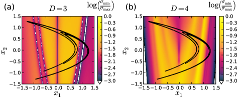
Figure 7: (Color online) Logarithm of ratio smallest singular value $\sigma_{min}=\sigma_{3}$ divided by largest singular value $\sigma_{max}=\sigma_{1}$ vs. $x_{1}$ and $x_{2}$ for the case of $M+P=3$ unknown $(x_{1},x_{2},p_{1}=a)$. The diagram shows the plane $p_{1}=a=1.4$ in the three dimensional estimation space. The other parameters are $b=0.3$ and $c=0.5$. Diagrams (a) and (b) show the results obtained with forward delay reconstruction dimensions $D=3$ and $D=4$, respectively.

Now we include $p_{2}=b$ in the list of quantities to be estimated. Figure 8 shows the ratio of singular values $\sigma_{min}/\sigma_{max}$ for reconstruction dimensions $D=4$ and $D=5$. For $D=4$ curves with very low singular value ratios $\sigma_{min}/\sigma_{max}$ exist crossing the Hénon attractor which disappear for $D=5$.

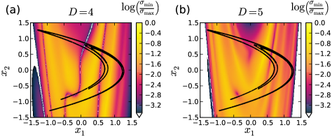
Figure 8: (Color online) Logarithm of the ratio of singular values $\sigma_{min}/\sigma_{max}=\sigma_{4}/\sigma_{1}$ vs. $x_{1}$ and $x_{2}$ for the case of $M+P=4$ unknown quantities $(x_{1},x_{2},p_{1}=a,p_{2}=b)$. The diagrams show the $x_{1}$-$x_{2}$ plane at fixed $p_{1}=a=1.4$ and $p_{2}=b=0.3$ in the four dimensional estimation space for $c=0.5$. Diagrams (a) and (b) show the results obtained with forward delay reconstruction dimensions $D=4$ and $D=5$, respectively.

Figure 9 shows the uncertainties $\nu_{1},\ldots,\nu_{4}$ (Eq. (27)) for $D=5$. As can be seen, the values of uncertainties vary strongly in the $x_{1}$-$x_{2}$ plane and still some islands with rather large uncertainties exist.

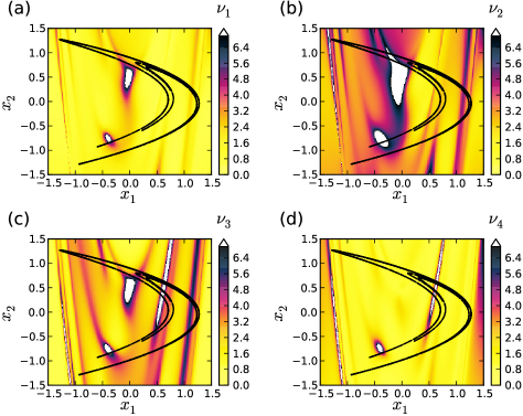
Figure 9: (Color online) Estimation of uncertainties $\nu_{j}$ ($j=1,\ldots,M=4)$) of variables $(x_{1},x_{2})$ and parameters $(p_{1}=a,p_{2}=b)$ of the Hénon map (8) obtained with $D=5$ dimensional forward delay coordinates .

Similar results are obtained if we include the remaining parameters $c$ in the estimation problem. Scanning the two-dimensional $x_{1}$-$x_{2}$ subspace (plane) of the $M+P=5$ dimensional estimation problem for $(\mathbf{x},\mathbf{p})=(x_{1},x_{2},p_{1},p_{2},q)$ with fixed $p_{1}=a=-1.4$, $p_{2}=b=0.3$, and $q=c=0.5$ indicates (almost) vanishing smallest singular values as long as $D\leq 8$. With $D=9$ dimensional delay coordinates the Jacobian matrix $DG(\mathbf{x},\mathbf{p})$ has clearly full rank almost everywhere within the chosen range $(x_{1},x_{2})\in[-1.,1.]\times[-1.,1.]$ as can be seen in Fig.. 10a. Figures 10b,c,d,e,f illustrate the uncertainties $\nu_{1},\ldots,\nu_{5}$ (Eq. (27)) of $x_{1},x_{2},p_{1},p_{2},q$, respectively.

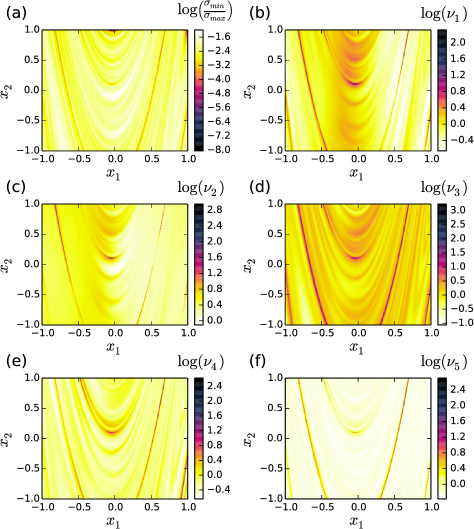
Figure 10: Estimation of all variables $\mathbf{x}=(x_{1},x_{2})$ and model parameters $\mathbf{p}=(p_{1},p_{2})=(a,b)$ of the Hénon map (8), and the measurement function parameter $q=c$ (FIR filter (10)). The output of the FIR filter is forward embedded in $D=9$ dimensions. (a) Ratio of smallest and largest singular value. (b)-(f) Uncertainties $\nu_{j}$ of state variables and parameters in the plane $\{(x_{1},x_{2},p_{1},p_{2},q):((x_{1},x_{2})\in[-1.,1.]\times[-1.,1.],p_{1}=a=1.4,p_{2}=b=0.3,q=c=0.5\}$.

.

II.6 Continuous dynamical systems

To compute the Jacobian matrix $DG({\mathbf{x}},\mathbf{p})$ (42) of the delay coordinates map $G$ we have to compute the gradients (43) and (44) of the observation function $s=h(\mathbf{x},\mathbf{q})$ and the Jacobian matrices $D_{x}\phi^{t}(\mathbf{x},\mathbf{p})$ and $D_{p}\phi^{t}(\mathbf{x},\mathbf{p})$ containing derivatives of the flow $\phi^{t}$ generated by the dynamical system (29) with respect to variables $x_{j}$ and parameters $p_{j}$, respectively. The $M\times M$-matrix $D_{x}\phi^{t}(\mathbf{x},\mathbf{p})$ can be computed by solving the linearized dynamical equations in terms of a matrix ODE

$$\frac{d}{dt}Y=D_{x}f(\phi^{t}(\mathbf{x},\mathbf{p}),\mathbf{p})\cdot Y$$ (47)

where $\phi^{t}(\mathbf{x},\mathbf{p})$ is a solution of Eq. (29) with initial value $\mathbf{x}$ and $Y$ is an $M\times M$ matrix that is initialized as $Y(0)=I_{M}$, where $I_{M}$ denotes the $M\times M$ identity matrix. Similarly, the $M\times P$-matrix $D_{p}\phi^{t}(\mathbf{x},\mathbf{p})$ is obtained as a solution of the matrix ODE Kawakami

$$\frac{d}{dt}Z=D_{x}f(\mathbf{x}(t),\mathbf{p})\cdot Z+D_{p}f(\mathbf{x}(t),\mathbf{p})$$ (48)

with $Z(0)=0$. Solving (47) and (48) simultaneously with the system ODEs (29) we can compute $D_{x}\phi^{\tau}(\mathbf{x})$, $D_{x}\phi^{2\tau}(\mathbf{x})$, etc. and use these matrices to obtain the Jacobian matrix $DG$ of the delay coordinates map $G$ (42). For mixed or backward delay coordinates the required components can be computed by integrating the system ODE and the linearized ODEs backward in time.

II.6.1 The Rössler system

To demonstrate the observability analysis for continuous systems we follow Aguirre and Letellier AL05 and consider the Rössler system

$$\dot{x}_{1} = -x_{2}-x_{3}$$

$$\dot{x}_{2} = x_{1}+ax_{2}$$ (49)

$$\dot{x}_{3} = b+x_{3}(x_{1}-c)$$

with $a=0.1$, $b=0.1$, and $c=14$.

Time series of different observables $x_{1}$, or $x_{2}$, or $x_{3}$ are considered, all of them consisting of $N=10000$ values sampled with $\Delta t=0.1$. Figure 11 shows the Rössler attractor where color indicates the uncertainty of estimating the variable $x_{1}$ (first column), or $x_{2}$ (second column), or $x_{3}$ (third column) using forward delay coordinates. The results in the first row are obtained when observing $x_{1}$, while the diagrams in the second and third row show results for $x_{2}$ or $x_{3}$ time series. The reconstruction dimension equals $D=7$ and the delay time is $\tau=0.5$. The bright yellow bullet indicates the state with the lowest uncertainty. This state and the $D-1=6$ following states plotted as thick red bullets underly the time series values that are used for the delay reconstruction. They span a window in time of length $(D-1)\tau=6\cdot 0.5=3$ which is about one half of the mean period of the chaotic oscillations $T\approx 6$. The lowest uncertainties are obtained for states whose reconstruction involves trajectory segments following the vertical $x_{3}$-excursion on the attractor. In contrast, trajectory segments starting from states with poor observability (large uncertainty) are located in the flat part of the Rössler attractor. Figures 11a and b show that using $x_{1}$ time series low values of $\nu_{1}$ occur on parts for the attractor where $\nu_{2}$ is high (and vice versa). Interestingly, this is not the case for delay reconstructions based on $x_{2}$ time series as can be seen in Figs. 11d and e, where low uncertainties of $x_{1}$ and $x_{2}$ occur in similar regions on the attractor.

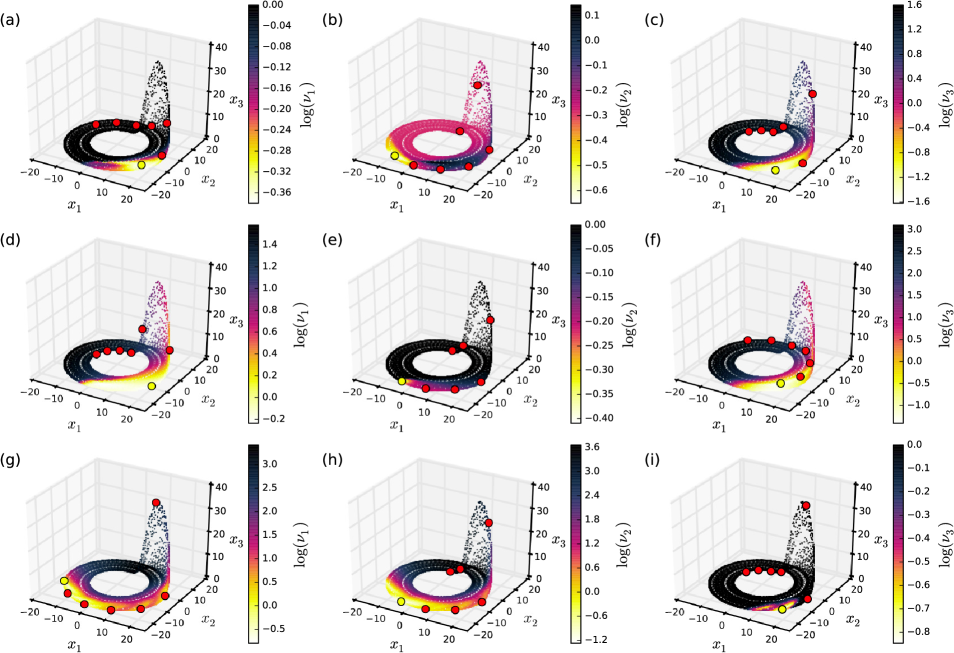
Figure 11: (color online) Color coded Rössler attractors where colors of points representing states are given by logarithms of uncertainty values $\nu_{1}$ in the first column, $\nu_{2}$ in the second column, and $\nu_{3}$ in the third column. All results are computed using forward delay coordinates. The diagrams in the first row show results obtained based on an reconstruction of a $x_{1}$ time series, the second row using $x_{2}$ as an observable, and the third row uncertainties of estimates from $x_{3}$ data. The reconstruction dimension is $D=7$ for all nine diagrams. The bright yellow bullet indicates the state with the lowest $\nu$-value (respectively). To estimate this state time series values at this state and at $D-1=6$ subsequent states indicated by dark (red) bullets are used for delay coordinates.

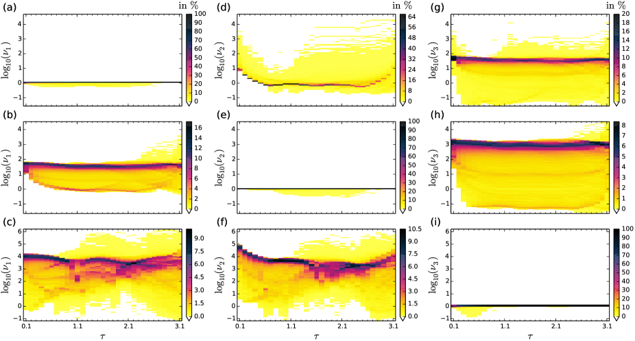
Figure 12: (Color online) Histograms of uncertainties $\nu_{j}$ of the Rössler system (49) vs. delay time $\tau$. All parameters are assumed to be known ($M=3$, $P=0$) and forward delay coordinates with dimension $D=4$ are used. In the first row a $x_{1}$ time series is given, in the second row $x_{2}$ data, and in the third row the delay reconstruction is based on $x_{3}$. The three columns show histograms of the (logarithm of the) uncertainties $\nu_{1}$, $\nu_{2}$, and $\nu_{3}$, respectively.

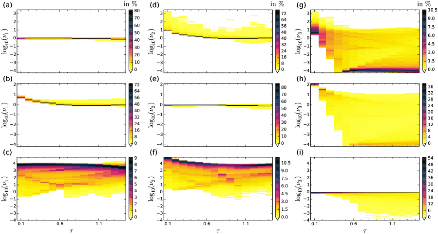
Figure 13: (Color online) Histograms of uncertainties $\nu_{j}$ of the Rössler system (49) vs. delay time $\tau$. All parameters are assumed to be known ($M=3$, $P=0$) and mixed delay coordinates with dimension $D=1+D_{-}+D_{+}=4$ are used ($D_{-}=1$, $D_{+}=2$). In the first row a $x_{1}$ time series is given, in the second row $x_{2}$ data, and in the third row the delay coordinates are based on $x_{3}$. The three columns show histograms of the (logarithm of the) uncertainties $\nu_{1}$, $\nu_{2}$, and $\nu_{3}$, respectively.

In Fig. 12 distributions of uncertainty values of the Rössler system are shown that were obtained along an orbit of $N=10000$ states sampled with $\Delta t=0.1$. The distributions are shown as color coded histograms, estimated from the relative frequency of occurrence of the corresponding $\nu_{j}$ (in %). All diagrams show the dependance of the histograms on the delay time $\tau$ chosen for forward delay coordinates (horizontal axis). The reconstruction dimension is for all cases $D=4$ and all three parameters are assumed to be known (and are not part of the estimation task, i.e. $P=0$). In the first row (Figs. 12a,d,g) estimations are based on a $x_{1}$ time series from the Rössler system, and in rows two and three, $x_{2}$ and $x_{3}$ time series are used, respectively. The uncertainties $\nu_{j}$ of the given observable $x_{j}$ (Figs. 12a,e,i) mostly equal one ($\log_{10}(\nu_{j})\approx 0$) or are smaller (due to the additional information provided by the delay coordinates). In general, lowest uncertainties for all variables are obtained when using $x_{1}$ time series (Figs. 12a,d,g) while $x_{3}$ data provide highest uncertainties (Figs. 12c,f,i).

Figure 13 shows the same diagrams but now computed using four dimensional mixed delay coordinates with $D_{-}=1$ and $D_{+}=2$. Similar to the results obtained with the Hénon map the uncertainties computed for mixed delay coordinates are typically smaller than those obtained with forward coordinates. Furthermore, the histograms shown in Fig. 13 suggest that for mixed delay coordinates using $x_{2}$ as measured variable provides the best results, followed by the $x_{1}$ time series. This is in contrast to forward coordinates (Fig. 12) where $x_{1}$ data yield the smallest uncertainties for the other variables ($x_{2}$ and $x_{3}$). Similar results have been obtained with three dimensional forward or mixed coordinates.

The fact that mixed delay coordinates provide the lowest uncertainties when using $x_{2}$ time series is consistent with results for derivative coordinates obtained by Letellier et al. LAM05 who found a ranking $x_{2}\rhd x_{1}\rhd x_{3}$ (for a different set of model parameters). For better comparison with their results we computed the (attractor) average

$$\bar{\gamma}=\frac{1}{T}\int_{0}^{T}\gamma(\mathbf{x}(t))dt$$ (50)

of the ratio

$$\gamma(\mathbf{x})=\frac{\sigma^{2}_{min}(DG(\mathbf{x}))}{\sigma^{2}_{max}(DG(\mathbf{x}))}$$ (51)

that provides the delay reconstruction analog $\bar{\gamma}$ of the observability index (4). Figure 14 shows $\bar{\gamma}$ vs. the delay time $\tau$ for different delay coordinates (rows) and different measured time series (columns). While for forward delay coordinates the largest values of the observability index occur if $x_{1}$ is measured (Fig. 14c), $x_{2}$ time series provide best observability if mixed delay coordinates are used (Fig. 14d). Note that in most cases high observability occurs for $\tau\approx 1$ which is very close to the first zero of the autocorrelation function (that is often used as preferred value for delay reconstruction).

Figure 14: Mean observability indices (50) of the Rössler system (49) vs. delay time $\tau$ based on three dimensional (dashed lines) and four dimensional (solid lines) delay coordinates. Left column ((a), (c), (e) forward delay coordinates. Right column ((b), (d), (f)) mixed delay coordinates with $D_{-}=1$ and $D_{+}=1$ (dashed lines) or $D_{+}=2$ (solid lines). The measured time series is in the first, second, and third row the variable $x_{1}$, $x_{2}$, and $x_{3}$, respectively.

Fig. 15 shows similar histograms but now for the full estimation problem ($M=3$ variables and $P=3$ parameters). Forward delay coordinates are used and the reconstruction dimension is increased to $D=13$ and an $x_{1}$ time series of length $N=10000$ is used (with sampling time $\Delta t=0.1$). For delay times $\tau$ that are an integer multiple of half of the mean period $T/2\approx 3$ relatively high uncertainties of occur, in particular for $\nu_{2}$, $\nu_{4}$, $\nu_{5}$, and $\nu_{6}$. This is due to the well known fact that for these delay times the attractor reconstruction results in points scattered near a straight (diagonal) line (an effect that also occurs when considering delay coordinates of a sinusoidal signal).

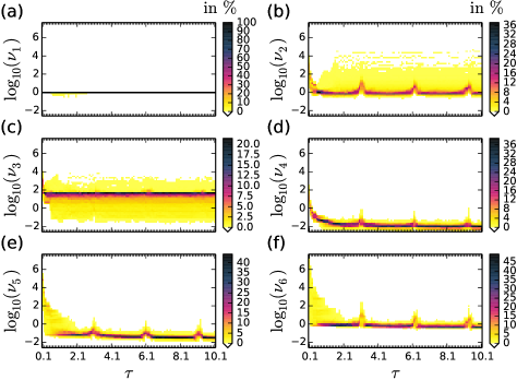
Figure 15: (color online) Histograms of uncertainties $\nu_{j}$ of the Rössler system (49) vs. delay time $\tau$. Both, all state variables ($M=3$) and all parameters ($P=3$) are assumed to be unknown and have to be estimated from a $x_{1}$ time series. Results are obtained using forward delay coordinates with $D=13$. The uncertainties $\nu_{1},\nu_{2},\nu_{3}$ correspond to state variables $x_{1}$, $x_{2}$, and $x_{3}$, while $\nu_{4},\nu_{5},\nu_{6}$ quantify uncertainties of estimated parameters $p_{1}$, $p_{2}$, and $p_{3}$.

III Conclusion

Starting from the question “Does some particular (measured) time series provide sufficient information for estimating a state variable or a model parameter of interest” we revisited the observability problem for nonlinear (chaotic) dynamical systems. In particular we considered delay coordinates and the ability to recover not measured state variables and parameters from delay vectors. This requires to “invert” the delay coordinates construction process which is at least locally possible, if the Jacobian matrix of the delay coordinates map has maximum (full) rank. Furthermore, we investigated how states near the delay vector are mapped back to the state and parameter space of the systems. In this way it is possible to quantify the amplification of small perturbations in delay reconstruction space in different directions of the state and parameter space. This reasoning gave rise to the concept of uncertainties of estimated variables and parameters. Both, observability and uncertainties may vary considerably in state space and on a given (chaotic) attractor. This feature was demonstrated with a discrete time system (filtered Hénon map) and a continuous system (Rössler system). Local observability and uncertainties also depend on the available measured variable (time series) and the type of delay coordinates. Best results were obtained with mixed delay coordinates, containing at least a one step backward in time.

The obtained information about (local) uncertainties in state and parameter estimation can be used in several ways for subsequent analysis. First of all, it may help to decide whether the planned estimation task is feasible at all or whether another observable has to be measured instead. For continuous time systems relevant time scales (delay times) can be identified where uncertainties are minimal.

The strong variations of local uncertainty values in state space (along a trajectory) occurring with the examples shown here are typical and should be taken into account by any estimation method. If the system is in a state where, for example, the uncertainty $\nu_{1}$ of the first variable is high then it might be better not to try to estimate this variable in this state or close to it, because the estimate might be poor and may spoil the overall results. Instead it makes more sense to wait until the trajectory enters a region of state space where $x_{1}$ can be estimated more reliably from the given time series.

The concrete implementation of such an adaptive approach depends on details of the estimation algorithm. For Newton-like algorithms, for example, it may consist of a simple strategy decreasing correction step sizes. Another potential application of uncertainty analysis is the identification of redundant parameters, i.e., parameter combinations that provide the same dynamical output.

- (1) H.U. Voss, J. Timmer, J. Kurths, Int. J. Bif. Chaos 14(6), 1905-1933 (2004).
- (2) A. Raue, V. Becker, U. Klingmüller, J. Timmer, Chaos 20, 045105 (2010).
- (3) H. Nijmeijer and I.M.Y. Mareels, IEEE Trans. Circuits Syst. I 44, 882-890 (1997).
- (4) H.J.C. Huijberts, T. Lilge, H. Nijmeijer, Int. J. Bif. Chaos 11(7), 1997-2006 (2001).
- (5) U. Parlitz, L. Junge and L. Kocarev, Phys. Rev. E 54, 6253-6529 (1996).
- (6) D. Ghosh and S. Banerjee, Phys. Rev. E 78, 056211 (2008).
- (7) H. D. I. Abarbanel, D.R. Creveling, J.M. Jeanne, Phys. Rev. E 77, 016208 (2008).
- (8) F. Sorrentino and E. Ott, Chaos 19, 033108 (2009).
- (9) I. G. Szendro, M. A. Rodríguez, and J. M. López, J. Geophys. Res. 114, D20109 (2009).
- (10) R. Konnur, Phys. Lett. A 346, 275-280 (2005).
- (11) U.S. Freitas, E.E.N. Macau, C. Grebogi, Phys. Rev.E 71, 047203 (2005).
- (12) M. Chen and J. Kurths, Phys. Rev. E 76, 027203 (2007).
- (13) R.E. Amritkar, Phys. Rev. E 80, 047202 (2009).
- (14) P.J. van Leeuwen, Q. J. R. Meteorol. Soc. 136, 1991-1999 (2010).
- (15) H.D.I. Abarbanel, Phys. Lett. A 373, 4044-4048 (2009).
- (16) J.C. Quinn, H.D.I. Abarbanel, Q. J. R. Meteorol. Soc. 136, 1855-1867 (2010).
- (17) D.R. Creveling, P.E. Gill, H. D. I. Abarbanel, Phys. Lett. A 372, 2640-2644 (2008).
- (18) J. Schumann-Bischoff and U. Parlitz, Phys. Rev. E 84, 056214 (2011).
- (19) J. Bröcker, Q. J. R. Meteorol. Soc. 136, 1906-1919 (2010).
- (20) E.D. Sontag, Mathematical Control Theory: Deterministic Finite Dimensional Systems, (Springer, New York,1998) 2nd ed.
- (21) H. Nijmeijer and A.J. van der Schaft, Nonlinear Dynamical Control Systems, (Springer,New York, 1990).
- (22) R. Hermann and A. J. Krener, IEEE Trans. Autom. Contr. AC-22(5), 728-740 (1977).
- (23) H. Nijmeijer, Int. J. Control 36(5), 867-874 (1982).
- (24) C. Letellier, L.A. Aguirre, and J. Maquet, Phys. Rev. E 71, 066213 (2005);
- (25) L. A. Aguirre and C.Letellier, J. Phys. A: Math. Gen. 38, 6311 - 6326 (2005).
- (26) C. Letellier, L.A. Aguirre, and J. Maquet, Comm. Nonl. Sci. Num. Sim. 11, 555-576 (2006).
- (27) C. Letellier and L.A. Aguirre, Phys. Rev. E 79, 066210 (2009).
- (28) M. Frunzete, J.-P. Barbot, and C. Letellier, Phys. Rev. E 86, 026205 (2012).
- (29) H. Kantz and T. Schreiber, Nonlinear Time Series Analysis, Cambridge Nonlinear Science Series 7, (Cambridge University Press, Cambridge, 1997).
- (30) H.D.I. Abarbanel, Analysis of Observed Chaotic Data, (Springer Verlag, 1997), 2nd ed.
- (31) T. Sauer, J.A. Yorke, and M. Casdagli J. of Stat. Phys. 65(3/4), 579-616 (1991).
- (32) D. Aeyels, SIAM J. Contr. Optimiz. 19(5), 595603 (1981).
- (33) F. Takens, Lect. Notes Math. 898, 366-381 (1981).
- (34) C. Letellier, L. A. Aguirre, and U. S. Freitas, Chaos 19, 023103, (2009).
- (35) U. Parlitz, J. Schumann-Bischoff, S. Luther, Phys. Rev. E 89, 050902(R), (2014).
- (36) J. Schumann-Bischoff, S. Luther, U. Parlitz, Commun. Nonlin. Sci. Num. Sim. 18(10) 2733 2742 (2013).
- (37) H. Kawakami, IEEE Trans. Circ. Syst. CAS-31(3), 248-260 (1984).