Estimation and uncertainty of reversible Markov models

Abstract

Reversibility is a key concept in Markov models and Master-equation models of molecular kinetics. The analysis and interpretation of the transition matrix encoding the kinetic properties of the model relies heavily on the reversibility property. The estimation of a reversible transition matrix from simulation data is therefore crucial to the successful application of the previously developed theory. In this work we discuss methods for the maximum likelihood estimation of transition matrices from finite simulation data and present a new algorithm for the estimation if reversibility with respect to a given stationary vector is desired. We also develop new methods for the Bayesian posterior inference of reversible transition matrices with and without given stationary vector taking into account the need for a suitable prior distribution preserving the meta-stable features of the observed process during posterior inference. All algorithms here are implemented in the PyEMMA software - http://pyemma.org - as of version 2.0.

I Introduction

Markov models, Markov state models (MSMs), or Master-equation models are a powerful framework to reduce the great complexity of bio-molecular dynamics to a simple kinetic description that represents the underlying transitions between distinct conformations Schütte et al. (1999); Swope, Pitera, and Suits (2004); Singhal, Snow, and Pande (2004); Schultheis et al. (2005); Noe et al. (2007); Pan and Roux (2008); Prinz et al. (2011). These models allow us to analyze the longest-living (metastable) sets of structures Deuflhard and Weber (2005), the effective transition rates between them Singhal and Pande (2005a); Noé et al. (2013), the kinetic relaxation processes and their relationship to equilibrium kinetics experiments Prinz et al. (2011); Noé et al. (2011); Zhuang et al. (2011); Keller, Prinz, and Noé (2012); Lindner et al. (2013), and the thermodynamics and kinetics over multiple thermodynamic states Sriraman, Kevrekidis, and Hummer (2005); Wu et al. (2014); Wu and Noé (2014); Rosta and Hummer (2015). A key advantage of MSMs is that they are estimated from conditional transition statistics between states, and they thus do not require the data to be in global equilibrium across all states. As a result, they are an excellent tool to integrate the data of multiple simulation trajectories that have been run independently and from different initial states into a single informative model Elmer, Park, and Pande (2005); Noé et al. (2009a); Buch, Giorgino, and De Fabritiis (2011).

A variety of complex molecular processes have been successfully described using MSMs. Examples include the folding of proteins into their native folded structure Noé et al. (2009a); Lane et al. (2011); Bowman, Voelz, and Pande (2011), the dynamics of natively unstructured proteins Perez-Hernandez et al. (2013a); Stanley, Esteban-Martin, and Fabritiis (2014), and the binding of a ligand to a target protein Held et al. (2011); Buch, Giorgino, and De Fabritiis (2011); Huang and Caflisch (2011); Silva et al. (2011); Bowman and Geissler (2012); Plattner and Noé (2015).

There are two key steps in the construction of a MSM. At first a suitable discretization of the continuous conformation space has to be obtained. In most cases no good a-priori discretization is known and the discretization has to be found based on the simulation data. The appropriate choice of discretization is a topic of ongoing research Chodera et al. (2007); Perez-Hernandez et al. (2013a); Schwantes and Pande (2013). The error incurred by the discretization and by the subsequent approximation of the jump-process as a Markov process can be systematically controlled and evaluated Sarich, Noé, and Schütte (2010); Prinz et al. (2011); Noé and Nüske (2013); Nüske et al. (2014).

In the second step one estimates the transition probabilities between pairs of states based on the transition statistics. The most common approach to estimating Markov models from data is by means of a Bayesian framework. One first harvests the transition counts, $c_{ij}(\tau)$ from the data, i.e. how often trajectories were found in discrete state $i$ at some time $t$ and in discrete state $j$ at some later time $t+\tau$. The parameter $\tau$ is called lag time and is crucial for the quality of the Markov model Sarich, Noé, and Schütte (2010); Prinz et al. (2011). Next, one computes the transition matrix either by maximizing the likelihood, i.e. the probability over all possible Markov model transition (or rate) matrices that may have generated the observed transition counts Buchete and Hummer (2008a); Bowman et al. (2009); Prinz et al. (2011); or by sampling Markov models from the posterior distribution Hinrichs and Pande (2007); Noé (2008); Chodera and Noé (2010); Schütte et al. (2011); Trendelkamp-Schroer and Noé (2013). A maximum likelihood estimate gives a single-point estimate, i.e. a single Markov model that is “most representative” given the data. However, if some transition events are rare compared to the total simulation length - and this is the typical case in molecular dynamics simulation - this maximum likelihood model might be very uncertain and thus far away from the model that the one would converge to by increasing amount of simulation data. The Bayesian posterior ensemble is a natural approach to quantify such statistical uncertainties and thus to make meaningful comparisons between a Markov models obtained from different sets of simulations, or to experimental data.

A key property of molecular dynamics at thermal equilibrium, and a necessary consequence of the second law of thermodynamics, is microscopic reversibility of the equations of motion. This property is ensured by many simulation procedures Van Gunsteren and Berendsen (1988); Tuckerman, Berne, and Martyna (1992) and carries over to detailed balance between discrete states, i.e. formally leads to a (time-) reversible Markov model. A reversible Markov model is not only physically desirable, it offers statistical advantages as it has only about half as many independent parameters compared to a nonreversible model, and it allows the equilibrium kinetics to be analyzed in a straightforward and meaningful manner. Furthermore imposing detailed balance with respect to a given stationary vector can be used to aid the efficient estimation of rare-event processes from MSMs Trendelkamp-Schroer and Noé (2014).

Algorithms imposing detailed balance during likelihood maximization have been discussed in Buchete and Hummer (2008b); Bowman et al. (2009); Prinz et al. (2011); Wu et al. (2014). First methods for the sampling the posterior distribution of reversible transition matrices have been suggested in Noé (2008) and later in Metzner, Noé, and Schütte (2009). A method working with natural priors for reversible chains was proposed in Bacallado, Chodera, and Pande (2009). The sampling of transition matrices reversible with respect to a fixed stationary distribution was also presented in Noé (2008), while a Gibbs sampling algorithm with a significantly improved convergence rate has been developed in Trendelkamp-Schroer and Noé (2013). Ref. Besag and Mondal (2013) discusses methods for goodness-of-fit tests for Markov chains.

This article is deliberately broad and presents new concepts, insights and algorithms for reversible Markov model estimation in general, maximum likelihood estimators and Bayesian estimators that mutually benefit from each other. For this reason we first give a survey of principles and consequences of reversible Markov models. We then extend the framework of maximum likelihood estimation of transition matrices by giving a simplified maximum likelihood estimator (MLE) for reversible transition matrices and a new estimator for reversible transition matrices with a fixed equilibrium distribution. The main part of the paper comprises new algorithms for the full Bayesian analysis of the posterior ensemble of reversible Markov models. As yet, three fundamental problems have not been satisfactorily solved: (i) How can one harvest statistically uncorrelated transition counts from trajectories in which subsequent transitions are correlated, so as to give rise to meaningful uncertainty intervals? (ii) Which prior should be used in a Bayesian analysis so as to get error intervals that envelop the true value even for Markov models with many states? (iii) How can we design efficient sampling algorithms for the reversible posterior ensemble, i.e. algorithms that allow to quickly compute reliable error bars for Markov models with many states? In this paper we discuss (i) give a rather complete treatment of problems (ii) and (iii). Efficient sampling algorithms are derived for reversible Markov models and reversible Markov models with fixed equilibrium distribution.

II Reversible Markov models

In this section we will show that microscopic reversibility carries over to the discretized situation and discuss the desirable properties of a reversible Markov state model.

II.1 From microscopic reversibility to discrete-state detailed balance

Let $\mu(x)$ denote the equilibrium distribution on the microscopic degrees of freedom $x\in\Omega$, e.g. all-atom coordinates of the system of interest, and let $p_{\tau}(x,y)$ denote the conditional transition density of the MD implementation. $p_{\tau}(x,y)$ is the probability that the system is found in state $y$ at time $t+\tau$ given that it has been in state $x$ at time $t$. The MD implementation fulfills microscopic reversibility if the following detailed balance equation

$$\mu(x)\,p_{\tau}(x,\,y)=\mu(y)\,p_{\tau}(y,\,x)$$ (1)

holds for all pairs of states $x,y\in\Omega$. Hence the terms “detailed balance” and “reversible” are equivalent in our context. Since $\mu(x)\,p_{\tau}(x,\,y)$ is the unconditional probability to find the transition $(x,\,t)\rightarrow(y,\,t+\tau)$, Eq (1) means that the system is on average time-reversible - the absolute number of transitions from $x$ to $y$ is equal to the reverse. Microscopic detailed balance is desirable to have in any MD implementation when the aim is to perform simulations in thermodynamic equilibrium. If the (1) would be violated, that would imply the existence of cycles $x\rightarrow y\rightarrow z\rightarrow x$ along which there is a net transport. Since such cycles could be used to generate work, their existence in a system that is driven by purely thermal energy would be inconsistent with the second law of thermodynamics.

Dynamical models that are commonly employed in MD implementations fulfill detailed balance. Brownian (overdamped Langevin) dynamics fulfills detailed balance. Hamiltonian and non-overdamped Langevin dynamics fulfill generalized detailed balance with respect to momentum inversion in phase space, but when integrating over the distribution of momenta they do fulfill ordinary detailed balance in position space Bittracher, Koltai, and Junge (Syst). In practice, some finite time-stepping integrators do not obey exact detailed balance with respect to the Boltzmann distribution, but we here consider that the MD implementation has been chosen such that detailed balance is at least approximately fulfilled.

Now suppose that the state space $\Omega$ is partitioned into non-overlapping subsets $S_{1},\,...,\,S_{n}$ that we shall call discrete states here. Each set has an equilibrium probability given by

$$\pi_{i}=\int_{S_{i}}\mathrm{d}x\,\mu(x)$$ (2)

and the transition density gives rise to a discrete state transition matrix $P(\tau)$ with entries

$$p_{ij}(\tau)=\frac{\int_{S_{i}}\mathrm{d}x\int_{S_{j}}\mathrm{d}y\,\mu(x)p_{\tau}(x,y)}{\int_{S_{i}}\mathrm{d}x\,\mu(x)}.$$ (3)

Using (2) and (3) and microscopic detailed balance, (1), it is straightforward to verify that

$$\pi_{i}p_{ij}(\tau)=\pi_{j}p_{ji}(\tau).$$ (4)

Note that (4) holds independently of the choice of the lag time $\tau$. Moreover, (4) implies that $\pi$ is the equilibrium probability vector of $P(\tau)$. By defining the diagonal matrix $\Pi=\mathrm{diag}(\pi_{1},\,...,\,\pi_{n})$, we can alternatively write (4) as a matrix equation:

$$\Pi P =(\Pi P)^{\top}$$ (5)

$$P =\Pi^{-1}P^{\top}\Pi$$ (6)

As a result, if the microscopic dynamics are reversible, the Markov model transition matrix must also be reversible. However, a direct estimate of $P$ from a finite amount of simulation data cannot be expected to fulfill (4) exactly. Thus, the principle validity of detailed balance motivates us to enforce (4) in the process of estimating $P$.

Enforcing detailed balance helps to reduce the statistical error of an estimator for $P$ because it reduces the number of independent variables roughly by approximately one half (see Table (1)). However, there are other consequences of having (4): Given detailed balance, we can compute the molecular equilibrium kinetics in a physically meaningful way and employ some useful analysis tools that are not defined for nonreversible Markov models. Moreover, we can employ more efficient and robust matrix algebra routines when exploiting that $P$ is a reversible matrix.

constraints	dof	$\approx$
none	$n(n-1)$	$n^{2}$
reversible	$\frac{1}{2}n(n-1)+n-1$	$\frac{1}{2}n^{2}$
reversible, fixed $\pi$	$\frac{1}{2}n(n-1)$	$\frac{1}{2}n^{2}$

Table 1: Number of independent variables (degrees of freedom, dof) and their approximated values for transition matrices depending on the constraints.

II.2 Eigenvalues and eigenvectors

Many methods to analyze the molecular kinetics based on a Markov model transition matrix rely on the eigenvalue decomposition of $P$. Using the diagonal eigenvalue matrix $\Lambda=\mathrm{diag}(\lambda_{1},\,...,\,\lambda_{n})$ we can formulate a right eigenvalue problem with right column eigenvectors $R=(r_{1},\,...,\,r_{n})$, $r_{i}\in\mathbb{R}^{n}$ and left row eigenvectors $L=(l_{1},\,...\,l_{n})^{\top}$:

$$PR =R\Lambda$$ (7)

$$LP =\Lambda L.$$ (8)

From (7), we can obtain a generalized eigenvalue problem:

$$\Pi PR=\Pi R\Lambda.$$

$\Pi$ is symmetric positive definite and as a result of detailed balance, $\Pi P$ is symmetric. Hence, all eigenvalues $\lambda_{1},\,...,\,\lambda_{n}$ are real, and the eigenvectors are orthogonal with respect to the equilibrium distribution Parlett (1998):

$$\langle r_{i},\,r_{j}\rangle_{\pi}\propto\delta_{ij},$$

where we have used the weighted scalar product $\langle u,v\rangle_{\pi}=\sum_{i}\pi_{i}u_{i}v_{i}$. We can make $R$ orthonormal by scaling an arbitrarily obtained eigenvector $r_{i}$ by $\langle r_{i},\,r_{i}\rangle_{\pi}^{-1/2}$.

Inserting the detailed balance formulation (6) into the decomposition (7) immediately gives:

$$P^{\top}\Pi R =\Pi R\Lambda$$

$$(\Pi R)^{\top}P =\Lambda(\Pi R)^{\top}$$

which is a left eigenvalue problem with the choice

$$L =(\Pi R)^{T}$$

$$l_{i}^{\top} =\Pi r_{i}.$$ (9)

Thus, detailed balance establishes a 1-to-1 relation between the left and the right eigenvectors. We can decompose the transition matrix into its spectral components by just using one set of eigenvectors and the equilibrium distribution, such as:

$$P=R\mbox{$\Lambda$}R^{\top}\Pi=\sum_{i=1}^{n}\lambda_{i}r_{i}r_{i}^{\top}\Pi.$$ (10)

Example 1:

Consider the following reversible $3\times 3$ transition matrix,

$$P=\left(\begin{array}[]{ccc}0.5&0.34&0.16\\ 0.28&0.5&0.22\\ 0.15&0.25&0.6\end{array}\right).$$ (11)

Suppose we generate a Markov chain of length $20$ starting from state 1, resulting in the count matrix at lag $\tau=1$:

$$C=\left(\begin{array}[]{ccc}4&3&0\\ 1&4&3\\ 1&1&2\end{array}\right).$$ (12)

Now we conduct a nonreversible and a reversible maximum likelihood estimation of the transition matrix given $C$. Eigenvalues for the exact transition matrix in (11) and both nonreversible and reversible estimates for the given count matrix in 12 are shown in Fig. 1.

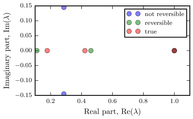
Figure 1: Eigenvalues of $3\times 3$ example system. The eigenvalues obtained from the reversible estimate (green) are a closer approximation to the true eigenvalues (red) than the eigenvalues obtained from the non-reversible estimate (blue). The unique eigenvalue $\lambda=1$ is faithfully reproduced by both estimates.

It is seen that the nonreversible estimate contains complex eigenvalues. These generally come in complex conjugate pairs. Fig. 1 shows a much higher accuracy of the reversible estimate compared to the nonreversible estimate. In order to explore the statistical significance of this observation, we run $N=1000$ chains of length $L=20$ using transition matrix (11). The reversible and nonreversible estimation results, together with the true eigenvalues, are reported below:

	$\lambda_{1}$	$\mathrm{Re}\{\lambda_{2}\}$	$\mathrm{Im}\{\lambda_{2}\}$	$\mathrm{Re}\{\lambda_{3}\}$	$\mathrm{Im}\{\lambda_{3}\}$
exact	1	0.42	0.0	0.18	0.0
rev	1	0.36$\pm$0.31	0.0	0.18$\pm$0.04	0.0
nonrev	1	0.32$\pm$0.29	-0.04$\pm$0.08	0.07$\pm$0.21	0.04$\pm$0.09

It is seen that the reversible estimates do not only have the correct real-valued structure, but can also have smaller uncertainties (here especially for $\lambda_{3}$). This is expected to be a general result due to the smaller number of degrees of freedom in the reversible estimate.

Example 2:

Fig. 2 shows the distribution of eigenvalues from nonreversible and reversible Markov models from simulation data for the alanine-dipeptide molecule (see Sec. V.2). The eigenvalues of the reversible estimate are purely real while the non-reversible estimate has eigenvalues with non-zero imaginary part.

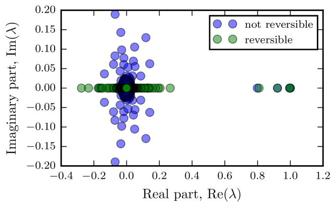
Figure 2: Eigenvalues for alanine dipeptide. The cluster of dominant eigenvalues indicates that the slowest processes are faithfully reproduced by the non-reversible (blue) as well as by the reversible (green) estimate. Only the eigenvalues of the reversible estimate are purely real.

II.3 Equilibrium kinetics analyses

Since detailed balance is a consequence of a system simulated at dynamical equilibrium, it is not surprising that detailed balance in the transition matrix $P$ is a prerequisite to analyze the equilibrium kinetics given $P$. Since kinetics are related to slow processes we will here only consider the $m$ largest eigenvalues $\lambda_{1},\,...\,\lambda_{m}$ and assume that they positive. Here are a few examples for equilibrium kinetics properties computed from reversible transition matrices:

1. The dominant relaxation rates of the molecular system are:

   $$\kappa_{i}=-\frac{1}{\tau}\ln\lambda_{i}$$ (13)

   where $i\geq 2$ ($i=1$ has a relaxation rate of zero and corresponds to the equilibrium distribution). The inverse quantities are the relaxation timescales $t_{i}=\kappa_{i}^{-1}$. These rates or timescales are of special interest because they are often detectable in kinetic experiments such as fluorescence time-correlation spectroscopy, two-dimensional IR spectroscopy or temperature jump experiments - see Noé et al. (2011) for a discussion.

2. The decomposition (10) can be used to write kinetic experimental observables in an illuminating form Noé et al. (2011); Keller, Prinz, and Noé (2012); Lindner et al. (2013). For example, the long-timescale part of the autocorrelation of a molecular observable $a\in\mathbb{R}^{n}$, e.g. containing the fluorescence values of every Markov state of a molecule, can be written as:

   $$\mathrm{acf}(a;\,\tau)\approx\langle a,\,\pi\rangle^{2}+\sum_{i=2}^{m}\langle a,\,r_{i}\rangle_{\pi}^{2}\mathrm{e}^{-\kappa_{i}\tau}$$ (14)

3. The PCCA+ method for seeking $m$ metastable sets of Markov states and its variants Deuflhard and Weber (2005); Röblitz and Weber (2013) assumes $m$ real-valued eigenvalues and eigenvectors. It is thus only reliably applicable to reversible transition matrices.

4. Discrete transition path theory Metzner, Schütte, and E. Vanden-Eijnden (2009); Noé et al. (2009b); Berezhkovskii, Hummer, and Szabo (2009) computes the statistics of transition pathways from a set of states $A$ to a set of states $B$ given a transition matrix. Discrete TPT can be used with nonreversible and reversible transition matrices. However, in the reversible case we get that the forward committor and the backward committor are complementary:

   $$q_{i}^{+}=1-q_{i}^{-}$$

   and the net fluxes, when ordering states such that $q_{i}^{+}\leq q_{j}^{+}$ are given by:

   $$f_{ij}^{+}=(q_{j}^{+}-q_{i}^{+})\pi_{i}p_{ij}$$

   which is analogous to an electric current $I=UG$ where $I=f_{ij}^{+}$, $U=(q_{j}^{+}-q_{i}^{+})$ is the potential difference and $\pi_{i}p_{ij}$ is the conductivity W. E and E. Vanden-Eijnden (2006).

III Likelihood, counting, and maximum likelihood estimation

We restate the transition matrix likelihood and formulate the maximum likelihood estimation problem for Markov model transition matrices. We present new estimation algorithms for reversible Markov models with known or unknown equilibrium distribution $\pi$.

III.1 Likelihood

Suppose we have a discrete sequence $S=\{s_{1},\,...,\,s_{N}\}$ with $s_{i}\in\{1,\,...,\,n\}$. If we assume that this sequence is the realization of a Markov chain with lag time $\tau=1$, the probability that a transition matrix $P$ has generated $X$ is proportional to the product of individual transition probabilities along the trajectory:

$$\mathbb{P}(S\mid P)\propto\prod_{t=1}^{N}p_{s_{t}s_{t+1}}$$ (15)

We have neglected the proportionality constant because we won’t need them in order to maximize or sample from (15). This is very handy because one component in this constant is the probability of generating the first state, $p_{s_{0}}$, which is often unknown, but is constant for a fixed data set $S$.

Suppose we have $c_{ij}$ transitions from $i$ to $j$. Then we can group all $p_{ij}$ terms together and get a factor $p_{ij}^{c_{ij}}$. Doing this for all pairs results in the equivalent likelihood formulation:

$$\mathbb{P}(C|P)\propto\prod_{i}\prod_{j}p_{ij}^{c_{ij}}$$ (16)

We can see that the count matrix $C\in\mathbb{R}^{n\times n}$ is a sufficient statistics for the Markov model likelihood $\mathbb{P}(S\mid P)$ - it generates the same likelihood although we have discarded the information in which sequence the transitions have occurred.

If multiple trajectories are available, their count matrices are simply added up.

III.2 Counting

How should we count transitions for longer lag times $\tau>1$, or if $S$ is not Markovian at lag time $\tau$? Regarding the first case, if $S$ is Markovian at lag time $\tau$, a safe approach seems to subsample the trajectory at time steps of $\tau$ and then treat the subsampled trajectory as above Singhal and Pande (2005a); Prinz et al. (2011). However this approach is statistically inefficient: If $S$ is also Markovian for shorter lag times than $\tau$, then we are using less information than we could. Even if $S$ only becomes Markovian at lag times of $\tau$ or longer, transitions such as $1\rightarrow\tau+1$ and $\tau/2\rightarrow\tau+\tau/2$ are usually only partially correlated, such that discarding the second transition is also not fully exploiting the data. In practical MD simulations, the lag times required such that a Markov model is a good approximation need to be quite long (often in the the range of nanoseconds), such that subsampling the data at $\tau$ will create severe problems with data and connectivity loss. Regarding the second case, if $S$ is not Markovian at lag time $\tau$ then treating every $c_{ij}$ as an independent count is incorrect.

Both cases can in principle be treated with the following formalism: We always obtain the count matrix $c_{ij}$ in a sliding window mode Prinz et al. (2011), i.e. we harvest all $N-\tau$ available transition counts from time pairs $(1\rightarrow\tau),\,(2\rightarrow\tau+1),\,...,\,(N-\tau\rightarrow N)$. Unless $S$ is Markovian at lag time 1, we will now harvest more transition counts than are statistically independent. We can formally correct for this by introducing a statistical inefficiency $I_{ij}(\tau)$ for every count at a given lag time, such that $c_{ij}^{\mathrm{eff}}(\tau)=I_{ij}(\tau)\,c_{ij}(\tau)$ is the effective number of counts, resulting in the likelihood

$$\mathbb{P}(C|P)\propto\prod_{i,\,j}p_{ij}^{c_{ij}^{\mathrm{eff}}}.$$ (17)

The determination of statistical inefficiencies for univariate signals is well established Janke (2002). Determining $I_{ij}(\tau)$ for transition count matrices is an open problem. A first approach that allows for the first time to estimate consistent, although somewhat too small uncertainty intervals for practical MD data is discussed in Noé (2015). Note that the validity of the estimation algorithms described in the present paper are independent of the choice of the count matrix, such that future methods for estimating the effective count matrix can be adopted without changing the estimation ablgorithms.

III.3 Maximum likelihood estimation

We will now assume that the effective counts are given. For better readability we will subsequently omit the superscript $\mathrm{eff}$ and just use $C=(c_{ij})$ to indicate counts. Now we ask the question what is the most likely transition matrix for the observation $C$, i.e. we seek the maximum likelihood estimate (MLE) that maximizes (15) over the set of transition matrices.

III.3.1 Non-reversible estimation

It is well known that the non-reversible MLE for the transition probability from state $i$ to state $j$ is simply given by the ratio of observed counts from $i$ to $j$ divided by the total number of outgoing transitions from state $i$ Anderson and Goodman (1957):

$$\hat{p}_{ij}^{\mathrm{nonrev}}=\frac{c_{ij}}{\sum_{k}c_{ik}}.$$ (18)

We use the hat in order to denote an estimator. The term non-reversible implies that reversibility has not been used as a constraint in the estimation of $\hat{P}^{\mathrm{nonrev}}$. Of course $\hat{P}^{\mathrm{nonrev}}$ can be coincidentally reversible and will be reversible if the count matrix $C$ is symmetric. For this reason, some early contributions in the field forced symmetry in $C$ by counting $S$ forward and backward. This practice is strongly discouraged as it will create a large bias unless the trajectories used are very long compared to the slowest timescales of the molecule.

III.3.2 Reversible estimation

Now we consider the problem of finding the reversible MLE $\hat{P}^{\mathrm{rev}}$ by enforcing detailed balance (4) with respect to an unknown equilibrium distribution $(\pi_{i})$ as constraint in the estimation procedure. Note that the count matrix used for this approach is not modified, i.e. it comes from a forward-only or nonreversible counting and is generally not symmetric. The constraints (4) can be more conveniently handled by defining the new set of variables

$$x_{ij}=\pi_{i}p_{ij}.$$ (19)

Note that

$$x_{i}=\sum_{j}x_{ij}=\pi_{i}.$$ (20)

We can thus recover the transition matrix from $X=(x_{ij})$ by:

$$p_{ij}=\frac{x_{ij}}{x_{i}}.$$ (21)

Inserting (21) into (16) and adding constraints for detailed balance and stochasticity leads to the reversible maximum likelihood problem:

$$\underset{X}{\text{maximize}} \sum_{i,j}c_{ij}\log\frac{x_{ij}}{\sum_{k}x_{ik}}$$ (22)

subject to $$X_{ij}=X_{ji}$$

$$\sum_{k}X_{ik}>0$$

$$X_{ij}\geq 0$$

Ignoring the inequality constraints the optimality conditions are

$$\frac{c_{ij}+c_{ji}}{x_{ij}}-\frac{c_{i}}{x_{i}}-\frac{c_{j}}{x_{j}}=0$$ (23)

with $c_{i}=\sum_{j}c_{ij}$ and $x_{i}=\sum_{j}x_{ij}$. There is no closed form solution when including the detailed balance constraint so that (22) has to be solved numerically. One option is to directly solve (23) for $x_{ij}$ and turn it into a fixed-point iteration, as first proposed in Bowman et al. (2009):

$$x_{ij}^{(k+1)}=\frac{c_{ij}+c_{ji}}{\frac{c_{i}}{x_{i}^{(k)}}+\frac{c_{j}}{x_{j}^{(k)}}}$$ (24)

where $k$ counts the iteration number in the algorithm. For a starting iterate $x_{ij}^{(0)}$ fulfilling the constraints in (22), for example $x_{ij}^{(0)}=(c_{ij}+c_{ji})/\sum_{i,j}(c_{ij}+c_{ji})$, the iterates will be symmetric and fulfill the inequality constraints for all $k>0$.

If we sum over $j$ on both sides of (24) and use (20), we can instead reduce the problem to iterative estimation of the equilibrium distribution:

$$\pi_{i}^{(k+1)}=\sum_{j=1}^{n}\frac{c_{ij}+c_{ji}}{\frac{c_{i}}{\pi_{i}^{(k)}}+\frac{c_{j}}{\pi_{j}^{(k)}}}$$ (25)

The iteration is terminated when $\lvert\lvert\pi^{(k+1)}-\pi^{(k)}|\rvert<\epsilon$ . The final estimate $\hat{\pi}$ is then inserted into (23) to recover the reversible transition matrix estimate:

$$\hat{p}_{ij}^{\mathrm{rev}}=\frac{(c_{ij}+c_{ji})\pi_{j}}{c_{i}\pi_{j}+c_{j}\pi_{i}}$$ (26)

Note that both the optimum sought by Eq. (25,26) exhibits $\hat{p}_{ij}=0$ if $c_{ij}+c_{ji}=0$. Thus, in both optimization algorithms, the sparsity structure of the matrix $\mathbf{C}+\mathbf{C}^{T}$ can be used in order to restrict all iterations to the elements that will result in a nonzero element $\hat{p}_{ij}>0$.

Furthermore, note that (25,26) are special cases of the transition-based reweighing analysis (TRAM) method - see Ref. Wu et al. (2014), Eqs (29-30) - for the special case of a single thermodynamic state. An example for the progress of the self-consistent iteration using an alanine dipeptide simulation is shown in Fig. 3.

A different method of iterative solution presented in Prinz et al. (2011) updates $x_{ij}$ with the exact solution to the quadratic problem arising from (23) while holding all other variables $x_{kl}$ fixed. As shown in Fig. 3, this approach can exhibit faster convergence properties than the fixed-point iteration (25).

Uniqueness of the estimator: The optimization problem (22) can be equivalently transformed into a convex optimization problem by replacing the decision variables $x_{ij}$ with $z_{ij}=\log(x_{ij})$ (see Wu and Noé (2014) for details), which implies the uniqueness of the maximum likelihood estimator.

a)

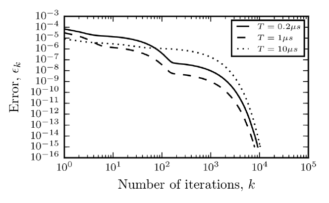
b)

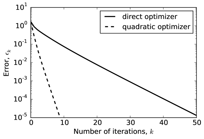
c)

Figure 3: Performance of algorithms for reversible maximum likelihood estimation. (a) Reversible transition matrix estimated using the fixed-point iteration (25) from an $n=228$ state count-matrix obtained from alanine-dipeptide simulation data. Convergence is shown for different total simulation lengths $T$. (b) Performance comparison of the direct fixed-point iteration (25) and the quadratic optimizer described in Ref. Prinz et al. (2011) for reversible transition matrix estimation given the count matrix $C=\left((5,\,2,\,0),\,(1,\,1,\,1),\,(2,\,5,\,20)\right)^{\top}$. Shown is the difference of the current likelihood to the optimal likelihood. (c) Same as b, but using the 1734$\times$1734 count matrix from Pin WW folding simulations used in Ref. Noé et al. (2009b).

III.3.3 Reversible estimation for given stationary vector

While unbiased MD simulations are useful to estimate state-to-state transition probabilities $p_{ij}$, enhanced sampling algorithms such as umbrella sampling and replica-exchange MD can be much more efficient in order to gain insight of the equilibrium distribution $\pi$. Ref. Trendelkamp-Schroer and Noé (2014) demonstrates how an uncertain estimate of $\pi$ can be combined with unbiased “downhill” trajectories in order to estimate rare event kinetics. A key in such a procedure is a way to estimate a reversible Markov model that is most likely given transition counts observed from MD simulations, but at the same time has a fixed equilibrium distribution $\pi$. Here we derive a new, efficient estimation algorithm for this task.

Enforcing reversibility with respect to a given stationary vector results in the following constrained optimization problem

$$\underset{P}{\text{maximize}} \sum_{i,j}c_{ij}\log p_{ij}$$ (27)

subject to $$\sum_{j}p_{ij}=1$$ (28)

$$p_{ij}\geq 0$$ (29)

$$\pi_{i}p_{ij}=\pi_{j}p_{ji}.$$ (30)

$\pi$ can only be the unique stationary distribution of $P$ if $P$ is irreducible. To ensure irreducibility, we restrict the state space to the largest (weakly) connected set of the undirected graph that is defined by the adjacency matrix $C+C^{T}$. For a system with $n$ states, Eqs (27,28,29,30) is a convex minimization problem in $\mathcal{\mathcal{{O}}}(n^{2})$ unknowns with $\mathcal{\mathcal{{O}}}(n^{2})$ equality and inequality constraints. Solving this with a standard interior-point method requires the solution of a linear system with $\mathcal{\mathcal{{O}}}(n^{2})$ unknowns to compute the search direction at each step. The resulting computational effort of $\mathcal{\mathcal{{O}}}(n^{6})$ operations for solving the linear system quickly becomes unfeasible for increasing $n$. Therefore we will propose a fixed-point iteration that is also feasible for large values of $n$.

To solve the maximization problem, we ignore the inequality constraint (29) at first. The row-stochasticity constraint (28) is enforced by introducing Lagrange multipliers $\lambda_{i}$ and adding penalty terms $\lambda_{i}\left(\sum_{j}p_{ij}-1\right)$ for all $i=1,\,...,\,n$ to the objective function. The detailed balance constraint (30) is included into the likelihood explicitly by the change of variables

$$p_{ij}^{\prime}=\begin{cases}p_{ij}&\text{if }i\leq j\\ \frac{\pi_{j}}{\pi_{i}}p_{ji}&\text{else}\end{cases}$$

These substitutions result in the Lagrange function:

$$\begin{split}F=\sum_{i}c_{ii}\log p_{ii}^{\prime}+\sum_{i<j}(c_{ij}+c_{ji})\log p_{ij}^{\prime}\\ -\sum_{i<j}p_{ij}^{\prime}\left(\lambda_{i}+\lambda_{j}\frac{\pi_{i}}{\pi_{j}}\right)-\sum_{i}\lambda_{i}p_{ii}^{\prime}+\sum_{i}\lambda_{i}+const\end{split}$$ (31)

that we seek to maximize. By setting the gradient of $F$ with respect to all $p_{ij}^{\prime}$ to zero and subsequently reversing the change of variables, we find the following expression for the maximum likelihood estimate

$$\hat{p}_{ij}=\frac{(c_{ij}+c_{ji})\pi_{j}}{\lambda_{i}\pi_{j}+\lambda_{j}\pi_{i}}$$ (32)

Note the similarity of this equation with the maximum likelihood result (26) where $\pi$ has been self-consistently computed from the counts. The row counts $c_{i}$ are here replaced by the yet unknown Lagrange multipliers $\lambda_{i}$. In order to find the Lagrange multipliers, we sum Eq. (32) over $j$:

$$\sum_{j}\frac{(c_{ij}+c_{ji})\pi_{j}}{\lambda_{i}\pi_{j}+\lambda_{j}\pi_{i}}=1$$ (33)

This doesn’t give a closed-form expression for $\lambda_{i}$. However, based on this equation, we propose the following fixed-point iteration for the Lagrange multipliers:

$$\lambda_{i}^{(n+1)}=\sum_{j,\ c_{ij}+c_{ji}>0}\frac{(c_{ij}+c_{ji})\lambda_{i}^{(n)}\pi_{j}}{\lambda_{j}^{(n)}\pi_{i}+\lambda_{i}^{(n)}\pi_{j}}.$$ (34)

Motivated by the analogy between Lagrange multipliers and row counts described above, we set the starting point to:

$$\lambda_{i}^{(0)}=\frac{1}{2}\sum_{j}(c_{ij}+c_{ji})$$ (35)

Taking the limit $\lambda_{i}\rightarrow 0^{+}$ in (34) still leads to a consistent solution. Choosing strictly positive starting parameters according to (35) results in valid iterates from (34). In analogy to the reversible case we iterate (34), (35) until $\left\|\lambda^{(k+1)}-\lambda^{(k)}\right\|<\epsilon$. An example for the progress of the self-consistent iteration using alanine dipeptide simulation data is shown in Fig. 4. Note that the converges is nearly three orders of magnitude faster compared to the estimation with unknown equilibrium distribution (Fig. 3).

Given converged Lagrange multipliers, we can exploit (32) to find the maximum likelihood transition matrix $\hat{P}$. For this algorithm the inequality constraints (29) are automatically fulfilled when $c_{ij}\geq 0$ for all $i,j$. Care must be taken in two situations: (i) $\lambda_{i}=\lambda_{j}=0$ - one can show that the simultaneous limit $\lambda_{i}\rightarrow 0^{+}$ and $\lambda_{j}\rightarrow 0^{+}$ can only occur for $c_{ij}+c_{ji}=0$, but then we know that $\hat{p}_{ij}=0$. (ii) A

diagonal element $c_{ii}$ is zero. Depending on the values of $\pi$, the solution $\lambda_{i}$ may take the value of zero such that equation (32) for $i=j$ becomes $\hat{p}_{ii}=c_{ii}/\lambda_{i}=0/0$ which is meaningless and is not the correct limit of $p_{ii}$ as $c_{ii}$ goes to zero. However this can be fixed easily by using $\hat{p}_{ii}=1-\sum_{j\neq i}\hat{p}_{ij}$. for the diagonal elements of $P$. In summary, we use the following equation for computing $\hat{P}$ from converged Lagrangian multipliers:

$$\hat{p}_{ij}=\begin{cases}\pi_{j}\frac{c_{ij}+c_{ji}}{\lambda_{i}\pi_{j}+\lambda_{j}\pi_{i}}&i\neq j,\>\lambda_{i}+\lambda_{j}\neq 0\\ 0&i\neq j,\>\lambda_{i}+\lambda_{j}=0\\ 1-\sum_{j\neq i}\hat{p}_{ij}&i=j\end{cases}$$ (36)

Uniqueness of the estimator: Since the above estimation algorithm is iterative, it is fair to ask whether the estimator $\hat{P}$ it converges to is unique, or whether there might be multiple local maxima that we could get stuck in. In this case, it is easy to show that the estimator is unique: Let $P^{*}$ be an optimal transition matrix. $p_{ij}^{*}=0$ exactly if $c_{ij}+c_{ji}=0$. Let $\Omega=\{p_{ij}|c_{ij}+c_{ji}>0\}$. Then, the function $f(P)=\sum_{i,j}c_{ij}\log p_{ij}$ is strictly convex on $\Omega$ and the constraints restrict the solution on a convex subset $\tilde{\Omega}\subset\Omega$. The minimization of a strictly convex function over a convex set has a unique solution.

Figure 4: Convergence of the reversible maximum likelihood estimation with fixed stationary vector. The transition matrix is estimated from an $n=228$ state count-matrix obtained from alanine-dipeptide simulation data. Convergence is shown for different total simulation lengths. The stationary distribution was obtained using the simple counting estimate, (83).

IV Bayesian estimation

We introduce new algorithms for sampling the full posterior probability distribution of Markov models, and in particular for estimating uncertainties of quantities of interest, such as relaxation timescales or mean first passage times. A key in these algorithms is the choice of a suitable prior which enforces the sampled matrices to have the same sparsity pattern as the transition count matrix, as this allows the credible intervals to lie around the true value even for large transition matrices. The relevance of the prior is first demonstrated for nonreversible Markov models, for which an efficient sampling algorithm is known. We then introduce new Gibbs sampling algorithms for reversible Markov models with and without constraints on the equilibrium distribution that vastly outperform previous algorithms for sampling reversible Markov models.

IV.1 Bayes theorem and Monte Carlo sampling

Bayes’ formula relates the likelihood of an observed effective count matrix $C$ given a probability model $P$ to the posterior probability of the model given the observation,

$$\underbrace{\mathbb{P}(P|C)}_{posterior}\propto\underbrace{\mathbb{P}(P)}_{prior}\underbrace{\mathbb{P}(C|P)}_{likelihood}.$$ (37)

The posterior accounts for the uncertainty coming from a finite observation. It incorporates a-priori knowledge about the quantity of interest using the prior probability $\mathbb{P}(P)$. We will see that a suitable choice of the prior is essential for the success of a Bayesian description for high-dimensional systems.

In general, if we are interested in an observable that is a function of a transition matrix, $f(P)$, we would like to compute its posterior moments, such as the mean and the variance,

$$\langle f\rangle =\int\mathrm{d}P\,\mathbb{P}(P|C)\,f(P),$$ (38)

$$\mathrm{Var}(f) =\int\mathrm{d}P\,\mathbb{P}(P|C)\,\left(f(P)-\langle f\rangle\right)^{2}.$$ (39)

While we usually use the maximum likelihood transition matrix $\hat{P}$ to provide “best” estimates, $f(\hat{P})$, the above integrals are of interest because $\sigma(f)=\sqrt{\mathrm{Var}(f)}$ gives us an estimate of the statistical uncertainty of $f$. Alternatively, we might be interested in the credible intervals which encompass the true value of $f$ with some probability, such as 0.683 ($1\sigma$ intervals) or 0.95 ($2\sigma$ intervals). As the integrals (38,39) are high-dimensional, we need to use Monte Carlo methods to approximate them.

In Monte Carlo methods we generate a sample of transition matrices $\{P^{(k)}\}_{k=1}^{N}$ distributed according to the posterior and evaluate $f$ at each element $P^{(k)}$ in the ensemble. We then approximate the posterior expectation value (38) and the posterior variance (39) by

$$m[f] =\frac{1}{N}\sum_{k=1}^{N}f(P^{(k)}).$$ (40)

$$s^{2}[f] =\frac{1}{N-1}\sum_{k=1}^{N}\left(f(P^{(k)})-m[f]\right)^{2}$$ (41)

Obtaining good and reliable samples of the posterior $\mathbb{P}(P|C)$ is very difficult. Previous approaches have suffered from some or all of the following difficulties, that are addressed here:

1. Choice of the prior: Given $n$ Markov states (typically 100s to 1000s), transition matrices have on the order of $n^{2}$ elements and are thus extremely high dimensional. Most priors used in the past allow to populate all these elements $p_{ij}$, including those for which no transition has been observed. Although the effect of the prior can be overcome by enough simulation data, for any practical amount of simulation data, such priors will lead to posterior distributions whose probability mass is far away from the $\hat{P}$ true model. This problem has been first addressed in Ref Noé et al. (2009a) by designing a prior that equates mean and MLE for nonreversible transition matrices, leading to credible intervals that nicely envelop the the true value. Here we design corresponding priors for reversible Markov models.

2. Uncorrelated transition counts $C$: As discussed in Sec. (III.2), the likelihood, and thus the posterior depends on how transition counts are harvested from the discrete trajectories which are generally time-correlated and not exactly Markovian at any particular lag time $\tau$. While the MLE is often not or little affected by the exact way of counting $C$, the uncertainties will be dramatically different if $C$ is e.g. counted in a sliding window mode (using transitions starting at all times $t=0,\,1,\,2,\,...$), or by subsampling the trajectory (using transitions starting at all times $t=0,\,\tau\,,2\tau$). Whereas the first approach underestimates the uncertainties, the second approach often overestimates them and is often not practical for large lagtimes $\tau$. Here we suggest to use the effective number of uncorrelated transition counts, $C=C^{\mathrm{eff}}$, and a first approach to compute them is described in Ref. Noé (2015).

3. Efficiency of the sampler: Finally, given a choice of prior and $C$, a sampling algorithm needs to explore the high-dimensional space of transition matrices in a reasonable time. This is especially problematic for reversible Markov models. The first Monte Carlo algorithm for sampling the reversible posterior, described in Ref. Noé (2008), suffers from poor mixing due to small acceptance probabilities of the individual steps. In Ref. Trendelkamp-Schroer and Noé (2013), an improved sampler was proposed. Here, we propose sampling algorithms for reversible Markov models with and without fixed equilibrium distribution whose efficiencies go far beyond previous approaches.

IV.2 Non-reversible sampling

Let us first illustrate the effect of prior choice on Bayesian estimation of nonreversible Markov models. A convenient functional form for the prior is the Dirichlet prior

$$\mathbb{P}(P)\propto\prod_{i}\prod_{j}p_{ij}^{b_{ij}}$$ (42)

where $B=(b_{ij})$ is a matrix of prior-counts. For this choice, the posterior is given by

$$\mathbb{P}(P|C)\propto\prod_{i}\left(\prod_{j}p_{ij}^{z_{ij}}\right).$$ (43)

$z_{ij}=c_{ij}+b_{ij}$ is the matrix of posterior pseudo-counts. In the non-reversible case we can generate independent samples from (43) by drawing rows of $P^{(k)}$ independently from Dirichlet distributions $\prod_{j}p_{ij}^{\alpha_{ij}-1}$ with Dirichlet parameters $\alpha_{ij}=z_{ij}+1=c_{ij}+b_{ij}+1$ Singhal and Pande (2005b).

Choosing a uniform prior, $b_{ij}=0$, assigns equal prior probability to all entries, $p_{ij}$, in the posterior ensemble. But this a-priori assumption can lead to serious problems when estimating quantities for meta-stable systems.

Consider for example the following transition matrix for a birth-death chain consisting of two meta-stable sets $A=\{1,\dotsc,m\}$, $B=\{m+2,\dotsc,n\}$, separated by a kinetic bottleneck in form of a single transition state,

$$P=\left(\begin{array}[]{ccccccccc}\frac{1}{2}&\frac{1}{2}&0\\ \frac{1}{2}&0&\frac{1}{2}\\ &\ddots&\ddots&\ddots\\ &&1-10^{-b}&0&10^{-b}\\ &&&\frac{1}{2}&0&\frac{1}{2}\\ &&&&10^{-b}&0&1-10^{-b}\\ &&&&&\ddots&\ddots&\ddots\\ &&&&&&\frac{1}{2}&0&\frac{1}{2}\\ &&&&&&&\frac{1}{2}&\frac{1}{2}\end{array}\right).$$ (44)

For barrier parameter $b=3$ and sets with $m=50$ and $n=101$ the expected time for hitting $B$ from state $x=1$ is $2\cdot 10^{5}$ steps. Now we are interested in the Bayesian estimator for a simulation of length $L=10^{7}$. The true distribution can be estimated with arbitrary precision by repeating the simulation many times. Here, $10^{3}$ repetitions led to an estimate of the 90% percentile for the mean first passage time of $[1.5,\,2.7]\cdot 10^{5}$ (see Table below).

In practice, we cannot afford to repeat the simulation many times but would like to approximate the true value and its statistical uncertainty from the given simulation data. Sampling the nonreversible posterior given expected counts for a single chain of length $L=10^{6}$ with a uniform prior, $b_{ij}=0$, results in non-zero transition probabilities for elements $p_{ij}$ which are zero in the true transition matrix. As a result artificial kinetic pathways circumventing the bottleneck are appearing in the posterior ensemble which lead to a dramatic underestimate of the mean first passage time. The Bayesian estimate with 90% credible interval obtained from $10^{3}$ posterior samples is $[1.9,\,2.0]\cdot 10^{3}$, and thus two orders of magnitude smaller than the true value $2\cdot 10^{5}$.

Using the prior $b_{ij}=-1$ suggested in Ref. Noé et al. (2009a) results in 90% credible intervals, $[1.5,2.7]\cdot 10^{5}$, which clearly cover the true value $2\cdot 10^{5}$. The choice $b_{ij}=-1$ leads to a posterior distribution in which sampled transition matrices $P$ have the same sparsity structure as the count matrix $C$, i.e. $p_{ij}=0$ if $c_{ij}=0$. As count matrices in the present context are generally sparse, we call this prior briefly sparse prior. Apparently the sparse prior leads to consistent credible intervals covering the true value.

method	estimate
true	$2.0_{1.5}^{2.7}\cdot 10^{5}$
uniform prior $b_{ij}=0$	$1.95_{1.9}^{2.0}\cdot 10^{3}$
sparse prior $b_{ij}=-1$	$2.0_{1.5}^{2.7}\cdot 10^{5}$

Fig. 5 shows the convergence of the 90% credible interval for the sparse and the uniform prior. The credible interval for the sparse prior envelopes the true value already given little data. To achieve consistency using the uniform prior requires simulations order of magnitudes longer than the timescale of the slowest process, thus rendering inference under this prior unpractical.

Note that our prior induces a fixed sparsity structure. This concept should not be confused with other sparsity inducing priors used i.e. in the context of Bayesian compressed sensing Ji, Xue, and Carin (2008), where the sparsity pattern is subject to uncertainty.

Figure 5: Convergence of the 90% credible interval for the sparse prior $b_{ij}=-1$ and the uniform prior $b_{ij}=0$. The dashed line indicates the true value. The credible interval for the improper prior covers the true value orders of magnitude before the credible interval for the uniform prior.

IV.3 A prior for reversible Markov models

Now we will present a new method for the sampling of reversible transition matrices. In our new approach we replace the Dirichlet prior (42) by a new prior for reversible sampling.

Similarly as in reversible maximum likelihood estimation, we define our reversible transition matrix sampler in the space of unconditional transition probabilities $x_{ij}$. For convenience we restrict ourselves to the independent set of variables with $i\leq j$ (remember that $x_{ij}=x_{ji}$ for reversible matrices), and keep them normalized to 1:

$$x_{ij} \propto\pi_{i}p_{ij}$$ (45)

$$\sum_{i\geq j}x_{ij} =1$$ (46)

Although $X$ is defined slightly different as in the maximum-likelihood case, the mapping from $X$ back to $P$ is still given by Eq. (21). We define a prior for reversible sampling on the set of $X$ matrices rather than on $P$: Choosing $x_{ij}$ as the set of independent variables has the advantage that obeying detailed balance amounts to sampling symmetric matrices, $X=X^{T}$.

$$\mathbb{P}(X)\propto\prod_{i\geq j}x_{ij}^{b_{ij}}.$$ (47)

The posterior for reversible sampling is then given by

$$\mathbb{P}(X|C)\propto\prod_{i\geq j}x_{ij}^{b_{ij}}\prod_{i,j}\left(\frac{x_{ij}}{\sum_{k}x_{ik}}\right)^{c_{ij}}$$ (48)

Below we will first consider how to sample from (48) using general prior counts $b_{ij}$. Then we will consider the specific choice $b_{ij}=-1$ for all $i\leq j$ and show that this choice has similar properties as the sparse prior in the nonreversible case.

IV.4 Sampling reversible transition matrices

There is no known method to generate independent samples from the posterior under the reversibility requirement. Instead we will use a a Markov chain Monte Carlo (MCMC) method to generate samples from the posterior ensuring that each sampled transition matrix fulfills the detailed balance condition (4). Our Markov chain will generate the ensemble $\{X^{(k)}\}_{k=1}^{N}$ via a set of updates advancing the chain from $X^{(k)}\rightarrow X^{(k+1)}$ starting from a valid initial state $X^{(0)}$. We can do a simple row-normalization of the $X$ matrices to obtain the desired ensemble $\{P^{(k)}\}_{k=1}^{N}$. Expectation values and variances will again be estimated using (40,41).

Similarly as in Noé (2008); Trendelkamp-Schroer and Noé (2013) we will construct our Markov chain using a Gibbs sampling procedure, where we sample a single element of $X$ in each step while leaving the other elements unchanged. We repeat this sampling procedure for every element of $X$, thus completing a Gibbs sweep. As detailed in the appendix, we can use the following general Gibbs step to sample the posterior (48):

1. Select an arbitrary element $x_{kl}$. Propose a new (unscaled) matrix $X\rightarrow X^{\prime}$ by sampling this element from the proposal density $q(x_{kl}^{\prime}|X)$:

   $$x_{ij}^{\prime}=\left\{\begin{array}[]{cc}\sim q(x_{kl}^{\prime}|X)&(i,j)=(k,l)\\ x_{ij}&\text{else}\end{array}\right.$$ (49)

   here $q(x_{kl}^{\prime}|X)$ is an arbitrary, scale-invariant density. Scale-invariance means that $q(x_{kl}^{\prime}|X)\propto q(cx_{kl}^{\prime}|cX)$ for any positive constant $c$.

2. Accept $\bar{X}^{\prime}$ as a new step in our Markov chain with probability $\min\{1,p_{acc}\}$ where

   $$p_{acc} =\left(1-x_{kl}+x_{kl}^{\prime}\right)^{-\frac{n(n+1)}{2}-b_{0}}\frac{q(x_{kl}|X^{\prime})}{q(x_{kl}^{\prime}|X)}\frac{\gamma(x_{kl}^{\prime}|X)}{\gamma(x_{kl}|X^{\prime})},$$

   where $b_{0}=\sum_{k\geq l}b_{kl}$ and $\gamma$ is the marginal density:

   $$\gamma(x_{kl}^{\prime}|X)\propto\left\{\begin{array}[]{ll}\frac{(x_{kk}^{\prime})^{c_{kk}+b_{kk}}}{(x_{k}-x_{kk}+x_{kk}^{\prime})^{c_{k}}},&k=l\\ \frac{(x_{kl}^{\prime})^{c_{kl}+c_{lk}+b_{kl}}}{(x_{k}-x_{kl}+x_{kl}^{\prime})^{c_{k}}(x_{l}-x_{kl}+x_{kl}^{\prime})^{c_{l}}},&k\neq l\end{array}\right.$$

3. Renormalize the matrix $X^{\prime}\rightarrow\bar{X}^{\prime}$ such that it fulfills (46):

   $$\bar{x}_{ij}^{\prime}=\frac{x_{ij}^{\prime}}{1-x_{kl}+x_{kl}^{\prime}}$$ (51)

While this approach will work for any choice of prior counts, we will now use the sparse prior $b_{ij}=-1$ for all $i,j$ with the hope to achieve similarly good results as in the nonreversible case. For this choice, $\gamma(x_{kl}^{\prime}|X)$ is scale-invariant, i.e. $\gamma(x_{kl}^{\prime}|X)=\gamma(cx_{kl}^{\prime}|cX)$, and the Jacobian pre-factor in (LABEL:eq:p_acc-reversible) is one. Thus we have:

$$p_{acc}=\frac{\gamma(x_{kl}^{\prime}|X)}{\gamma(x_{kl}|X^{\prime})}\frac{q(x_{kl}|X^{\prime})}{q(x_{kl}^{\prime}|X)}$$ (52)

Thus the ideal choice of the proposal density is $q\equiv\gamma$, which would guarantee that the acceptance probability is always $1$. This proposal density degenerates to a point probability at zero if $c_{kl}+c_{lk}=0$, which implies $b_{ij}=-1$ encodes a priori belief that any transition for which neither the forward direction nor the backward direction has ever been observed in the data has zero probability in the posterior ensemble. Thus, this prior enforces $P$ to have the same sparsity structure as the count matrix, like the choice $b_{ij}=-1$ for nonreversible sampling. Note that the reversible MLE has the same sparsity structure as can be seen from the update rule (24).

We will choose proposal densities $\gamma(x_{kl}^{\prime}|X)$ that are also scale-invariant. In this case the normalization step 3 above ($X^{\prime}\rightarrow\bar{X}^{\prime}$) can be omitted, i.e. if we accept $X^{\prime}$, we can directly set it as our new sample $X^{(k)}$ and obtain $P^{(k)}$ by row normalization. We will now outline how to design the proposal density $\gamma$ such that the acceptance probability is 1 or nearly 1. For $k=l$, sampling $x_{kk}^{\prime}\sim\gamma(x_{kk}^{\prime}|X)$ is equivalent to sampling the following transformed variable (see Appendix):

$$s^{\prime}=\frac{x_{kk}^{\prime}}{x_{k}-x_{kk}+x_{kk}^{\prime}}\sim\mathrm{Beta}(c_{kk},c_{k}-c_{kk})$$ (53)

So we can simply define $q(x_{kk}^{\prime}|X)\equiv\gamma(x_{kk}^{\prime}|X)$ and generate $x_{kk}^{\prime}$ by

$$s^{\prime} \sim \mathrm{Beta}(c_{kk},c_{k}-c_{kk})$$

$$x_{kk}^{\prime} = (x_{k}-x_{kk})\frac{s^{\prime}}{1-s^{\prime}}$$ (54)

For $k\neq l$, there is no known way to draw independent samples, but $\gamma(x_{kl}^{\prime}|X)$ can be well approximated by a Gamma distribution by matching the maximum point and the second derivative at the maximum. A Gamma distribution can be efficiently sampled and we use it as proposal density and accept the resulting $x_{kl}^{\prime}$ with probability $\min\{1,p_{acc}\}$. Specifically, our proposal step is:

$$x_{kl}^{\prime}\sim\gamma(x_{kl}^{\prime}|X)=\mathrm{Gamma}(x_{kl}^{\prime}|\alpha,\,\beta)$$ (55)

with the parameters

$$\alpha =-h\bar{v}$$ (56)

$$\beta =-h\bar{v}^{2}$$ (57)

using

$$\bar{v} =\frac{-b+\sqrt{b^{2}-4ac}}{2a}$$ (58)

$$h =\frac{c_{k}}{(\bar{v}+x_{k}-x_{kl})^{2}}+\frac{c_{l}}{(\bar{v}+x_{l}-x_{kl})^{2}}-\frac{c_{kl}+c_{lk}}{\bar{v}^{2}}$$ (59)

$$a =c_{k}+c_{l}-c_{kl}-c_{lk}$$ (60)

$$b =(c_{k}-c_{kl}-c_{lk})(x_{l}-x_{kl})+(c_{l}-c_{kl}-c_{lk})(x_{k}-x_{kl})$$ (61)

$$c =-(c_{kl}+c_{lk})(x_{k}-x_{kl})(x_{l}-x_{kl})$$ (62)

which matches the value and the first two derivatives of the true marginal density at the maximum (see Appendix for derivation), and leads to acceptance probabilities close to one for most values of $x_{kl}$. However, if the current value of $x_{kl}$ is in one of the heavy tails of the distribution $\gamma(x_{kl}^{\prime}|X)$, the acceptance probability can be much less than 1 and the Markov chain can get stuck. In order to avoid this problem, we utilize a second step to generate $x_{kl}^{\prime}$: After we sample $x_{kl}^{\prime}$ from the proposal density (55) we sample $x^{\prime}_{kl}$ according to:

$$\log x_{kl}^{\prime}\sim\mathcal{N}(\log x_{kl}^{\prime}|\log x_{kl},1)$$ (63)

where $\mathcal{N}(x|m,\,s)$ denotes the Normal distribution of $x$ with mean $m$ and standard deviation $s$. The proposal density defined by the above update is

$$\tilde{q}(x_{kl}^{\prime}|X)=\frac{1}{x_{kl}}\mathcal{N}(\log x_{kl}^{\prime}-\log x_{kl}|0,1),$$ (64)

and the corresponding acceptance probability is:

$$p_{acc}=\frac{\gamma(x_{kl}^{\prime}|X)}{\gamma(x_{kl}|X)}\frac{x_{kl}^{\prime}}{x_{kl}}$$ (65)

In summary, the proposed Algorithm 1 is a Metropolis within Gibbs MCMC algorithm with adapted proposal probabilities for each Gibbs sampling step. For efficiency reasons, transition matrix elements $(i,\,j)$ for which no forward- or backward transition counts have been observed, can be neglected in the sampling algorithm, in order to account for the effect of the sparse prior.

Input: $C$, $X^{(j)}$

Output: $X^{(j+1)}$

for all indexes $(k,\,l)$ with $k\leq l$ and $c_{kl}+c_{lk}>0$ do

     if $k=l$ then

           Sample $x_{kk}^{(j+1)}$ from (54)

          

           end if

          else

                Calculate $\alpha$ and $\beta$ by (56,57), and sample $x_{kl}^{\prime}$ from $\mathrm{Gamma}(\alpha,\,\beta)$.

               $p_{acc}=\frac{\gamma(x_{kl}^{\prime}|X)}{\gamma(x_{kl}|X)}\frac{\mathrm{Gamma}(x_{kl}|\alpha,\beta)}{\mathrm{Gamma}(x_{kl}^{\prime}|\alpha,\beta)}$

                Accept $x_{kl}^{\prime}$ as $x_{kl}^{(j+1)}$ with probability $\min\{1,p_{acc}\}$

                Sample $x_{kl}^{\prime}$ by $\log x_{kl}^{\prime}\sim\mathcal{N}(\log x_{kl},1)$.

               $p_{acc}=\frac{\gamma(x_{kl}^{\prime}|X)}{\gamma(x_{kl}|X)}\frac{x_{kl}^{\prime}}{x_{kl}}$

                Accept $x_{kl}^{\prime}$ as $x_{kl}^{(j+1)}$ with probability $\min\{1,p_{acc}\}$

                end if

               

                end for

Algorithm 1 Reversible sampling algorithm

IV.5 A prior for reversible Markov models with fixed equilibrium distribution

As before we will be working with variables $x_{ij}=\pi_{i}p_{ij}$ related to transition matrix entries $p_{ij}$ via (45). In contrast to the previous algorithm, $\pi$ is not a function of $P$ but fixed. Thus the single normalization condition (46) is replaced by a condition for each row:

$$\sum_{j}x_{ij}=\pi_{i},$$ (66)

in order to ensure reversibility with respect to the given $\pi$.

All $x_{kl}$ in the lower triangle ($k>l$) are used as independent variables. Given a valid $X$ matrix, an update that respects the constraints is given by

$$x_{kl} \rightarrow x^{\prime}_{kl}$$ (67a)

$$x_{kk} \rightarrow x_{kk}+(x^{\prime}_{kl}-x_{kl})$$ (67b)

$$x_{lk} \rightarrow x^{\prime}_{kl}$$ (67c)

$$x_{ll} \rightarrow x_{ll}+(x^{\prime}_{lk}-x_{lk}).$$ (67d)

(67b) and (67d) ensure that the normalization condition (66) holds for the new sample and will thus keep $$\pi P X x_{kl}^{\prime}$$ constant, while (67c) restores the symmetry and thus ensures reversibility of . We will again use the prior (47) defined on the set of matrices and sample from the posterior (48). The ideal proposal density of is

$$\gamma(x_{kl}^{\prime}\mid X)\propto (x_{kl}^{\prime})^{c_{kl}+c_{lk}+b_{kl}}\left(x_{kk}+x_{kl}-x_{kl}^{\prime}\right)^{c_{kk}+b_{kk}}$$

$$\left(x_{ll}+x_{kl}-x_{kl}^{\prime}\right)^{c_{ll}+b_{ll}}$$ (67e)

which is the conditional distribution density for given all off-diagonal elements of $$X x_{kl} \pi C$$ (except ), and the counts .

We have seen that a correct choice of prior parameters was essential in order to successfully apply the posterior sampling for meta-stable systems. As in the reversible case we will use $b_{kl}=-1$ for $k>l$ to enforce $x_{kl}=0$ whenever $c_{kl}+c_{lk}=0$.

However, the choice of prior counts for the diagonal elements $b_{kk}$ is less straightforward. According to our experience, a good choice is to determine the value of $b_{kk}$ based on the maximum likelihood estimate $\hat{p}_{kk}$ of the $k$-th diagonal element as

$$b_{kk}=\begin{cases}0&\>\>\>\>\>\hat{p}_{kk}>0,c_{kk}=0\\ -1&\>\>\>\>\>\mathrm{else}\end{cases}$$ (68)

which ensures that the posterior expectation of $p_{kk}$ is zero if and only if $\hat{p}_{kk}=0$, and the conditional expectation of (67e),

$$\mathbb{E}(x_{kl}^{\prime}\mid X)=\frac{c_{kl}+c_{lk}}{c_{kl}+c_{lk}+c_{ll}}(x_{ll}+x_{kl})$$ (69)

matches the MLE of the one-dimensional likelihood function for $x_{kl}$ given $X$ if $\hat{p}_{kk}>0$ and $c_{kk}=0$. (Note that for the MLE of $P$, there is at most one $k$ which satisfies $\hat{p}_{kk}>0$ and $c_{kk}=0$ - see proof in Appendix.)

However, in the case that $\hat{p}_{kk}=0$, the conditional (67e) would then degenerate so that $x_{kk}^{\prime}=0$ with probability one, and the $k$-th row and column of $X$ would remain fixed in the sampling process. This effect can break ergodicity in the sampled Markov chain and therefore prevent convergence of the algorithm. This problem is avoided by regularizing the prior choosing the prior parameter as $b_{kk}=-1+\epsilon$ for $\hat{p}_{kk}=0$ such that (67e) does not degenerate, where $\epsilon>0$ is a small number. In addition we need to ensure that the Markov chain is started from an initial state $X^{(0)}$ with $x_{kk}^{(0)}>0$. In summary, we select the prior of $X$ for reversible sampling with fixed $\pi$ as

$$b_{kk}=\begin{cases}0&\>\>\>\>\>\hat{p}_{kk}>0,c_{kk}=0\\ -1+\epsilon&\>\>\>\>\>\hat{p}_{kk}=0,c_{kk}=0\\ -1&\>\>\>\>\>c_{kk}>0\end{cases}$$ (70)

This choice of prior will again ensure that $c_{kl}+c_{lk}=0$ results in $p_{kl}=0$ and $p_{lk}=0$ for all $k<l$ and for all posterior samples, a property shared by the reversible MLE with fixed stationary vector. This ensures that the posterior mass is located around the maximum likelihood estimate $\hat{P}$ and again prevents the occurrence of artificial kinetic pathways in the posterior ensemble.

IV.6 Sampling reversible Markov models with fixed equilibrium distribution

We now investigate how to efficiently sample the conditional (67e). Here we assume without loss of generality that $x_{kk}<x_{ll}$ and transform $x_{kl}^{\prime}\in(0,\,x_{kk}+x_{kl})$ into a new variable $v^{\prime}\in(0,+\infty)$ via

$$v^{\prime}=\frac{x_{kl}^{\prime}}{x_{kk}+x_{kl}-x_{kl}^{\prime}}.$$ (71)

The ideal proposal density of $v^{\prime}$ is then

$$\gamma_{v}(v^{\prime}|X) \propto \left|\frac{\partial x_{kl}^{\prime}}{\partial v^{\prime}}\right|\gamma(x_{kl}^{\prime}|X)$$ (72)

$$= \left(v^{\prime}\right)^{c_{kl}+c_{lk}+b_{kl}}\left(\frac{s}{s-1}+v^{\prime}\right)^{c_{ll}+b_{ll}}$$

$$\cdot\left(1+v^{\prime}\right)^{-\left(c_{kl}+c_{lk}+c_{kk}+c_{ll}+b_{kl}+b_{kk}+b_{ll}+2\right)}$$

$$= \left(v^{\prime}\right)^{a_{1}}\left(\frac{s}{s-1}+v^{\prime}\right)^{a_{3}}\left(1+v^{\prime}\right)^{-\left(a_{1}+a_{2}+a_{3}\right)}$$

with

$$s = \frac{x_{ll}+x_{kl}}{x_{kk}+x_{kl}}$$

$$a_{1} = c_{kl}+c_{lk}+b_{kl}$$

$$a_{2} = c_{kk}+b_{kk}$$

$$a_{3} = c_{ll}+b_{ll}$$

Like in the previous algorithm, we can approximate the conditional of $v$ by a Gamma distribution as:

$$\gamma_{v}(v^{\prime}|X)\approx\mathrm{Gamma}(v^{\prime}|\alpha,\,\beta)$$ (73)

with

$$\alpha =-h\bar{v}$$ (74)

$$\beta =-h\bar{v}^{2}$$ (75)

and

$$\bar{v} =\frac{-b+\sqrt{b^{2}-4ac}}{2a}$$ (76)

$$h =-\frac{a_{1}}{\bar{v}^{2}}-\frac{a_{3}}{\left(\frac{s}{s-1}+\bar{v}\right)^{2}}+\frac{a_{2}}{\left(1+\bar{v}\right)^{2}}$$ (77)

$$a =a_{2}+1$$ (78)

$$b =a_{2}-a_{1}+\frac{a_{2}+a_{3}+1}{s-1}$$ (79)

$$c =\frac{s\left(a_{1}+1\right)}{1-s}$$ (80)

See Appendix for derivation. Then $v^{\prime}$ can be sampled by a Metropolis sampling step with the proposal density $\mathrm{Gamma}(v^{\prime}|\alpha,\beta)$ and the acceptance ratio

$$\min\{1,p_{acc}\}=\min\left\{1,\frac{\gamma_{v}(v^{\prime}|X)\mathrm{Gamma}(v|\alpha,\beta)}{\gamma_{v}(v|X)\mathrm{Gamma}(v^{\prime}|\alpha,\beta)}\right\}$$

where $v=x_{kl}/x_{kk}$ denotes the original value of $v$. In addition, in order to avoid the sampler from getting stuck at an extremely small or large value of $v$, we also utilize the same strategy as in Section IV.4 to generate $v^{\prime}$ by

$$\log v^{\prime}\sim\mathcal{N}(\log v^{\prime}|\log v,1)$$

.

The proposed Algorithm 2 for sampling of reversible transition matrices with fixed stationary vector can again be characterized as a Metropolis within Gibbs MCMC algorithm with adapted proposal probabilities.

Input: $C$, $\pi$, $X^{(j)}$

Output: $X^{(j+1)}$

for all indexes $(k,\,l)$ with $k<l$ and $c_{kl}+c_{lk}>0$ do

     if $x_{kk}<x_{ll}$ then

          $v=\frac{x_{kl}}{x_{kk}}$

          $s=\frac{x_{ll}+x_{kl}}{x_{kk}+x_{kl}}$

           $a_{1}=c_{kl}+c_{lk}+b_{kl}$

          $a_{2}=c_{kk}+b_{kk}$

          $a_{3}=c_{ll}+b_{ll}$

           end if

          else

               $v=\frac{x_{kl}}{x_{ll}}$

               $s=\frac{x_{kk}+x_{kl}}{x_{ll}+x_{kl}}$

               $a_{1}=c_{kl}+c_{lk}+b_{kl}$

               $a_{2}=c_{ll}+b_{ll}$

               $a_{3}=c_{kk}+b_{kk}$

                end if

               Calculate $\alpha$ and $\beta$ by (74) and (75)

                Sample $v^{\prime}$ from $\mathrm{Gamma}(\alpha,\beta)$.

               Let $x_{kl}^{\prime}=\min\{x_{kk}+x_{kl},x_{ll}+x_{kl}\}\cdot\frac{v}{1+v}$.

               $p_{acc}=\frac{\gamma_{v}(v^{\prime}|X)\mathrm{Gamma}(v|\alpha,\beta)}{\gamma_{v}(v|X)\mathrm{Gamma}(v^{\prime}|\alpha,\beta)}$ using (67a)-(67d)

               Accept $x_{kl}$ as $x_{kl}^{(j+1)}$ with probability $\min\{1,p_{acc}\}$

               Sample $v^{\prime}$ by by $\log v^{\prime}\sim\mathcal{N}(\log v,1)$.

               $p_{acc}=\frac{\gamma_{V}(v^{\prime}|X)v^{\prime}}{\gamma_{V}(x_{kl}|X)v}$

               Let $x_{kl}^{\prime}=\min\{x_{kk}+x_{kl},x_{ll}+x_{kl}\}\cdot\frac{v}{1+v}$.

                Accept $x_{kl}^{\prime}$ as $x_{kl}^{(j+1)}$ with probability $\min\{1,p_{acc}\}$

                end for

Algorithm 2 Reversible sampling algorithm with fixed stationary vector

V Results

V.1 Validation

We first demonstrate the validity of the reversible sampling algorithm for the following $2\times 2$ count-matrix,

$$C=\left(\begin{array}[]{cc}5&2\\ 3&10\end{array}\right).$$ (81)

In Fig. 6 we compare the sampled histograms using Algorithm 1 with analytical values for the non-reversible posterior with Dirichlet-prior-counts $b_{ij}=-1$. Any $2\times 2$ transition matrix automatically fulfills detailed balance, and therefore the analytical and sampled densities are expected to be equal. The histogram for samples of the reversible algorithm are indeed in agreement with the analytical posterior.

Figure 6: Sampled histogram frequency (a) and analytical probability density (b) of reversible posterior for $2\times 2$ count matrix. Sampled frequencies are in agreement with the analytical probabilities.

In Fig. 7 the sampled histogram for count matrix (81) with fixed stationary distribution $\pi=\left(0.25,\,0.75\right)^{\top}$ using Algorithm 2 is compared with the exact posterior distribution. The detailed balance relation (4) with fixed stationary vector enforces a linear dependency between the transition matrix element $p_{12}$ and $p_{21}$. The resulting posterior is therefore restricted to the line $\pi_{1}p_{12}=\pi_{2}p_{21}$ such that the projection on $p_{12}$ in Fig. 7 already contains the full information about the one-dimensional posterior. A comparison between histogram frequency and analytical density demonstrates the validity of the algorithm.

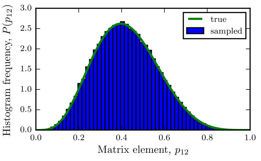
Figure 7: Sampled histograms and analytical probability density for reversible posterior with fixed stationary vector for $2\times 2$ count-matrix.

V.2 Applications

To demonstrate the usefulness of the proposed algorithms we apply them to molecular dynamics simulation data. Here, two systems are chosen to illustrate our methods: (1) The alanine-dipeptide molecule, and (2) the bovine pancreatic trypsin inhibitor molecule (BPTI).

We start by discussing the alanine dipeptide results. The system was simulated on GPU-hardware using the OpenMM simulation package Eastman et al. (2013) using the amber99sb-ildn forcefield Lindorff-Larsen et al. (2010) and the tip3p water model Jorgensen et al. (1983). The cubic box of length $2.7nm$ contained a total of $652$ solvent molecules. We used Langevin equations at $T=300K$ with a time-step of $2fs$. A total of $10\mu s$ of simulation data was generated. The $\phi$ and $\psi$ dihedral angles were discretized using a $20\times 20$ regular grid to obtain a matrix of transition counts $C=(c_{ij})$, here by sampling one count per lag time $\tau$. Below we will show histograms for two important observables, largest implied time-scales $t_{i}$ and expected hitting times, $\tau(A\rightarrow B)$, for pairs $A$, $B$ of meta-stable sets. We compute the posterior sample-mean and 90% credible intervals for $1\mu s$ of simulation data and show that the credible intervals nicely envelop a reference value obtained from the MLE transition matrix for the total simulation data, supporting the proposed prior as a ’good’ choice for reversible sampling in meta-stable systems.

V.2.1 Alanine dipeptide, reversible sampling

In Fig. 8 we show histograms of implied time-scales computed from a reversible posterior sample. The mean values estimated from the posterior sample are in good agreement with the reference values. Tables 2 and 3 compare the reference values with the sample mean $\mu$ and sample standard deviation $\sigma$ for each observable.

In order to gain a first impression of the efficiency of the sampling and the quality of our estimates, we compute the integrated autocorrelation time $t_{corr}$ for each quantity sampled (here implied timescales and hitting times). The error of the sample mean $m[f]$ compared to the true mean $\langle f\rangle$ can then be estimated as

$$\epsilon=\mathbb{E}[(m[f]-\langle f\rangle)^{2}]=\frac{\sigma^{2}[f]}{N_{\mathrm{eff}}}$$ (82)

where $N_{\mathrm{eff}}=N/(1+2t_{corr})$ is the effective number of samples with $N$ the total number of samples. See Ref. Geyer (1992) for a thorough discussion. $t_{corr}$ and $\epsilon$ are also reported in Table (2).

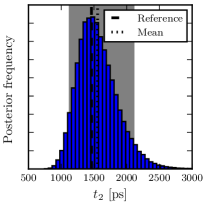
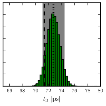
(a) (b) (c)

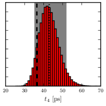
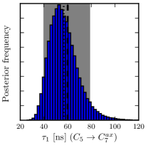
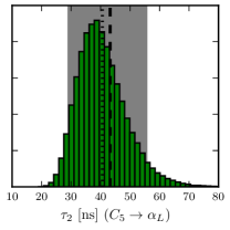
(d) (e) (f)

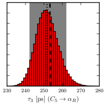
Figure 8: a)-c) Implied time-scales, $t_{i}$. Histograms obtained from reversible posterior sampling. Dashed lines indicate the reference value, $\hat{t}_{i}$, dotted lines indicate the posterior sample mean, $\mu(t_{i})$. MLE and posterior mean are in very good agreement for the proposed choice of prior. The 90% credible intervals are the shaded regions in gray. Expected hitting times, $\tau$, d)-f). Histograms obtained from reversible posterior sampling. Dashed lines indicate the reference value, $\hat{\tau}$, dotted lines indicate the posterior sample mean, $\mu(\tau)$. In all cases the reference value obtained from a long simulation is clearly compatible with the posterior sample (credible interval).

	$\hat{t}_{i}/ps$	$\mu/ps$	$\sigma/ps$	$\epsilon/ps$	$t_{corr}$
$t_{2}$	1462	1556	303	19.00	197
$t_{3}$	71	73	1	0.01	10
$t_{4}$	36	43	5	0.06	7

Table 2: Comparison of reference implied time-scales ($\hat{t}_{i}$) with mean $\mu$ and standard deviation $\sigma$ from the reversible posterior using $N=10^{5}$ samples. $\epsilon$ is the estimated error of the mean $\mu$ and $t_{\mathrm{corr}}$ is the autocorrelation time of the sampled quantity.

Fig. 8d-f) show histograms for expected hitting times for the three transitions $C_{5}\rightarrow C_{7}^{ax}$, $C_{5}\rightarrow\alpha_{L}$ and $C_{5}\rightarrow\alpha_{R}$ between meta-stable sets in the $\phi$ and $\psi$ dihedral angle plane. Again, mean values are in good agreement with the corresponding reference values. Table (3) summarizes the computed results. The table columns again contain the reference value $\hat{\tau}$ the mean value $\mu$, the standard deviation $\sigma$, the estimated correlation time $t_{corr}$ and the error of the mean value, $\epsilon$.

	$\hat{\tau}/ns$	$\mu/ns$	$\sigma/ns$	$\epsilon/ns$	$t_{corr}$
$\tau(C_{5}\rightarrow C_{7}^{ax})$	60.4	56.7	12.0	0.77	202
$\tau(C_{5}\rightarrow\alpha_{L})$	43.6	40.6	8.3	0.53	206
$\tau(C_{5}\rightarrow\alpha_{R})$	0.253	0.250	0.005	0.0004	218

Table 3: Expected hitting times computed from reversible posterior using $N=10^{5}$ samples. See Table 2 for definition of other symbols.

V.2.2 Alanine dipeptide, reversible sampling with fixed equilibrium distribution

Below we report results for sampling with fixed stationary distribution. The stationary distribution $\pi_{i}$ was, for sake of simplicity, computed using the relative frequencies of state occurrences,

$$\pi_{i}=\frac{\sum_{k}c_{ik}}{\sum_{j,k}c_{jk}}.$$ (83)

It should be noted that a more useful and independent source of $\pi$ are enhanced sampling simulations targeted at rapidly generating a good estimate of the equilibrium probabilities alone. See Ref. Trendelkamp-Schroer and Noé (2014) for methods and applications that combine MD simulations and enhanced sampling simulations in order to efficiently compute rare-event kinetics.

Results are shown in In Table 4 and Fig. 9. The sample mean is again in good agreement with the reference value. For the computatio of the reference value we use the MLE transition matrix of the full simulation data reversible with respect to the input stationary distribution for the posterior sampling. The additional constraint imposed by fixing the stationary distribution is clearly reflected in smaller standard deviations for all shown observables compared to the reversible case.

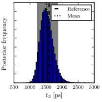
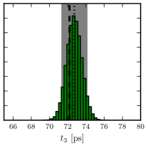
(a) (b) (c)

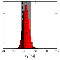
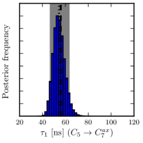
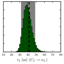
(d) (e) (f)

Figure 9: a)-c) Implied time-scales, $t_{i}$. Histograms obtained from reversible posterior sampling with fixed stationary vector. Dashed lines indicate the reference value, $\hat{t}_{i}$, dotted lines indicate the posterior sample mean, $\mu(t_{i})$. The 90% credible intervals are the shaded regions in gray. d)-f) Expected hitting times $\tau$. Histograms obtained from reversible posterior sampling with fixed stationary vector. Dashed lines indicate the reference value, $\hat{\tau}$, dotted lines indicate the posterior sample mean, $\mu(\tau)$. The reference value obtained from a long simulation is clearly compatible with the posterior sample (credible interval) in all cases except the .

	$\hat{t}_{i}/ps$	$\mu/ps$	$\sigma/ps$	$\epsilon/ps$	$t_{corr}$
$t_{2}$	1594	1520	196	0.6	1
$t_{3}$	72	73	1	0.003	1
$t_{4}$	38	41	3	0.01	1

Table 4: Comparison of reference implied time-scales , ($\hat{t}_{i}$), with mean $\mu$ and standard deviation $\sigma$ from the reversible posterior using a fixed equilibrium distribution and $N=10^{5}$ samples. $\epsilon$ is the estimated error of the mean $\mu$ and $t_{\mathrm{corr}}$ is the autocorrelation time of the sampled quantity.

Histograms for expected hitting times between meta-stable sets are shown in Fig. 9d-f). The sample mean is again in good agreement with the reference value. Again, we summarize our results, c.f. Table 5.

	$\hat{\tau}/ns$	$\mu/ns$	$\sigma/ns$	$t_{corr}$	$\epsilon/ns$
$\tau(C_{5}\rightarrow C_{7}^{ax})$	56.0	54.5	5.0	1	0.02
$\tau(C_{5}\rightarrow\alpha_{L})$	41.5	39.5	5.1	1	0.02
$\tau(C_{5}\rightarrow\alpha_{R})$	0.249	0.251	0.003	1	$9.7\cdot 10^{-6}$

Table 5: Expected hitting times computed from reversible sampling with fixed stationary vector using $N=10^{5}$ samples. See Table 4 for the definition of symbols.

V.2.3 Bovine pancreatic trypsin inhibitor, reversible sampling

For BPTI, we used the 1 ms simulation generated on the Anton supercomputer Shaw et al. (2010). Please refer to that paper for system setup and simulation details. We prepared data as follows: $C_{\alpha}$ atom positions were oriented to the mean structure and saved every 10 ns, resulting in about 100,000 configurations with 174 dimensions. Time-lagged independent component analysis (TICA) Perez-Hernandez et al. (2013b); Schwantes and Pande (2013) was applied to reduce this 174-dimensional space to the two dominant IC’s as a spectral gap was found after the second nontrivial eigenvalue. $k$-means clustering with $k=100$ was used to discretize this space.

Effective count matrices were obtained using the method described in Noé (2015) at a range of lag times up to 2 $\mu$s. Fig. 10 shows the implied relaxation timescales obtained from a maximum likelihood estimate with values comparable to the Hidden Markov model analysis in Ref. Noé et al. (2013). The figure also shows uncertainties computed from a reversible transition matrix sampling as described above with $N=1000$ samples. Only every $20$th transition matrix sample was used to compute timescales in order to reduce the computational effort to $50$ eigenvalue decompositions. It is seen that the MLE is nicely contained in the 2$\sigma$ (95%) credible interval. The entire transition matrix sampling for Fig. 10 took about 12.5 seconds on a 1.7 GHz Intel Core i7. Given that 8 lag times were used for $1000$ samples of $100\times 100$ matrices that contained about 40% non-zeros, about 2.56 million elements are sampled per second, and about 640 full transition matrix samples are generate per second. Below a more systematic analysis of the computational efficiency is made.

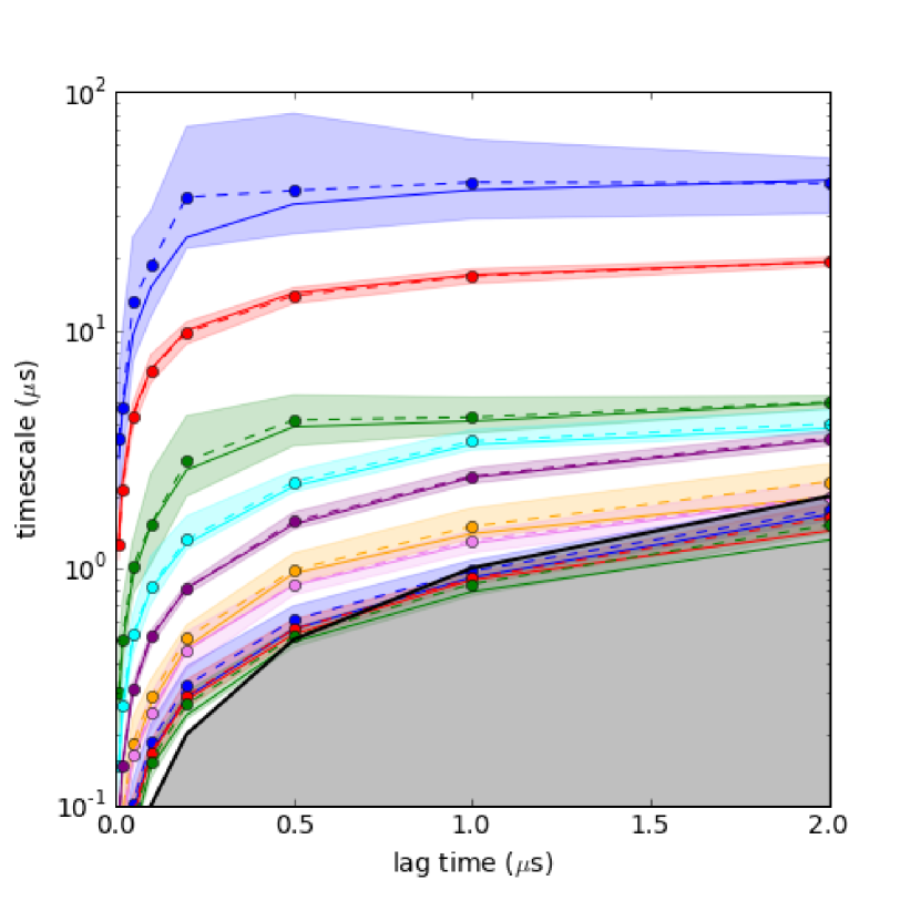
Figure 10: Implied timescales for a Markov model of bovine pancreatic trypsin inhibitor (BPTI). The error bars are 95% confidence intervals estimated using the reversible transition matrix sampling algorithm described here using transition counts as described in Ref. Noé (2015).

V.3 Efficiency

We compute acceptance probabilities of the Metropolis-Hastings steps and compare the statistical efficiency of the proposed sampling algorithm with the algorithm proposed in Ref. Noé (2008) that uses uniform proposal densities. Efficiency is measured in terms of achieved autocorrelation times for sampling of transition matrices with different sizes. As a representative observable we choose the largest relaxation time-scale $t_{2}$ for the alanine dipeptide molecule and compute autocorrelation functions and autocorrelation times from a large sample of size $N=10^{6}$. Two differently fine discretizations were used, resulting in $n\times n$-shaped transition matrices with $n=258$ and $n=1108$.

Fig. 11 shows autocorrelation functions for the second largest relaxation time-scale, $t_{2}$, for a reversible posterior ensemble. The autocorrelation function for the reversible sampling algorithm with posterior adapted proposals shows a much faster decay than the autocorrelation function for the algorithm in Ref. Noé (2008). Table 6 compares acceptance probabilities and autocorrelation times. The present proposal steps lead to very high acceptance probabilities, $p>0.99$, for the sampling off-diagonal entries. The main advance, however comes from the fact that the step for sampling diagonal transition matrix elements in Ref. Noé (2008) has suffered from a very poor acceptance probability. As that step was the only step that modified the equilibrium distribution, the sampler in Ref. Noé (2008) has very poor mixing properties. In contrast, our current algorithm generates independent samples for the diagonal elements, resulting in an acceptance probability of $p=1.0$.

The autocorrelation times for the new sampler are more than a factor 5 shorter for the small (233 state) matrix and more than a factor 13 shorter for the large (1108 state) matrix, indicating a much higher efficiency of the new approach. The autocorrelation time of the new algorithm increases only mildly for matrices of increased dimension, indicating that the present algorithm will be useful for very large Markov models.

(a)

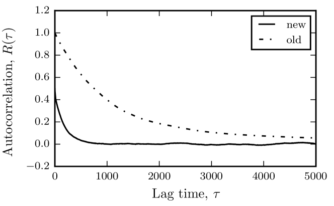
(b)

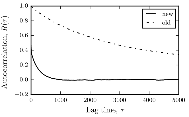
Figure 11: Autocorrelation function for reversible sampling. Sampling of transition matrices with $n=233$ states, a), and b) with $n=1108$ states. Increasing the dimension of the state space has only a small effect on the new sampling algorithm.

algorithm	$n$	$p_{\text{offdiag}}$	$p_{\text{diag}}$	$t_{\text{corr}}$
old	233	0.216	0.011	1088.1
	1108	0.271	0.005	3241.9
new	233	0.994	1.0	194.7
	1108	0.995	1.0	242.6

Table 6: Acceptance probability and autocorrelation times for old vs. new reversible sampling algorithm. $n$: number of states; $p_{\mathrm{offdiag}}$, $p_{\mathrm{diag}}$: acceptance probabilities for off-diagonal and diagonal elements, respectively. $t_{\mathrm{corr}}$: Autocorrelation time for the sampling of the slowest relaxation timescale, in number of transition matrix sampling steps.

Fig. 12 shows autocorrelation functions for reversible sampling with fixed stationary vector. The posterior adapted proposals in reversible sampling algorithm with fixed stationary distribution again result in a much faster decay of the autocorrelation function than the uniform proposals of the algorithm in Ref. Noé (2008). Table 7 compares acceptance probabilities and autocorrelation times for the two algorithms. For sampling with fixed stationary vector there is no sampling step for the diagonal elements. Although the average acceptance probabilities are only a factor of 3-4 better for our new algorithm, the autocorrelation times are decreased by a factor 35 for the small system (233 states) and over a factor 300 for the large system (1108 states). Again, there is only a mild increase in autocorrelation time when the dimension of the sampled space is increased.

(a)

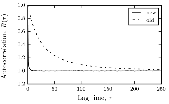
(b)

Figure 12: Autocorrelation function for reversible sampling with fixed stationary distribution. Sampling of transition matrices with $n=233$ states, a), and b) with $n=1108$ states. Increasing the dimension of the state space has only a small effect on the new sampling algorithm.

algorithm	$n$	$p_{\text{offdiag}}$	$t_{\text{corr}}$
old	233	0.175	72.096
	1108	0.230	$>1000$
new	233	0.752	2.893
	1108	0.706	3.157

Table 7: Acceptance probability and autocorrelation times for old vs. new reversible sampling algorithm with fixed stationary distribution. Symbols as in Table 6.

VI Conclusion

In this work we have described and significantly extended the state of the art in reversible Markov model estimation. Reversible Markov models are expected to naturally arise from molecular dynamics implementations that fulfill microscopic reversibility. Reversibility is an essential property in order to analyze the equilibrium kinetics of a molecule. However, in order to have reversibility in a Markov model, it needs to be enforced in the estimation procedure. When done correctly, reversible estimation does not bias the model but rather reduces statistical errors as a result of a smaller number of degrees of freedom.

We have presented minor improvements to an existing self-consistent estimation algorithm for reversible Markov models. Then we have presented a new and efficient algorithm to estimate reversible maximum likelihood Markov models given a fixed equilibrium distribution.

The main part of the presented work focuses on the long-standing problem of Bayesian estimation of the posterior ensemble of reversible transition matrices. Although several algorithms to sample reversible Markov models have been presented in the past, they have been hampered by three fundamental problems, two of which are addressed here: (i) Which prior should be chosen such that the posterior is located around the true value rather than completely elsewhere? (ii) How should transition counts be obtained when time series are correlated and not really Markovian at any given lag time $\tau$? (iii) How can the sampling algorithm be made efficient such that also large transition matrices can be sampled in reasonable time?

To address problem (i), we develop priors that ensure that reference values and sample mean are similar. The key property of these priors is that they make the a priori assumption that transitions between states that have not been sampled in the trajectory in either direction, have zero probability. This is a sparse prior, i.e. an improper prior enforcing that the sampled transition matrix has the same sparsity structure as the maximum likelihood estimate and as induced by the observation. In contrast to most other priors that have been previously suggested, these sparse priors achieve the desired property of creating errors bars that nicely envelop the reference estimates.

For problem (ii), we have described the principles of how it can be addressed. We suggest that effective count matrices are obtained using the concept of statistical inefficients. A separate preprint Noé (2015) suggests an initial solution towards this aim that is successfully applied on simulation data of the bovine pancreatic trypsin inhibitor in the present paper. The solution of problem (ii) is still in its infancy and needs further investigation..

For problem (iii), we present highly efficient Gibbs sampling algorithms for reversible transition matrices and reversible transition matrices with fixed equilibrium distribution. Both methods are demonstrated to have acceptance probabilities close to 1 in their individual update steps. Autocorrelation times from samples of the slowest relaxation timescale are one or two orders of magnitude shorter than with a previous Gibbs sampling algorithm, indicating a high statistical efficiency of our sampler.

Implementations of all algorithms described here are available in PyEMMA Scherer et al. (sion) as of version 2.0 or later - www.pyemma.org .

Appendix A Details for transition matrix sampling

A.1 Reversible transition matrix sampling: derivation of marginal densities

We first pick a single element $(k,\,l)$ of $X$ (diagonal or off-diagonal) and sample it from a proposal density $x_{kl}^{\prime}\sim q(x_{kl}^{\prime}|X)$ that is scale-invariant with $q(x_{kl}^{\prime}|X)\propto q(cx_{kl}^{\prime}|cX)$ for all $c>0$:

$$x_{ij}^{\prime}=\left\{\begin{array}[]{ll}\sim q(x_{kl}^{\prime}|X),&(i,j)=(k,l)\\ x_{ij},&\text{else}\end{array}\right.$$ (84)

and then renormalize the matrix such that it retains an element sum of 1:

$$\bar{x}_{ij}^{\prime}=\frac{x_{ij}}{1-x_{kl}+x_{kl}^{\prime}}$$ (85)

Since $q(x_{kl}^{\prime}|X)$ is a probability density function, we can obtain from its scale-invariance that

$$\int q(cx_{kl}^{\prime}|cX)\mathrm{d}x_{kl}^{\prime} = \frac{1}{c}\int q(cx_{kl}^{\prime}|cX)\mathrm{d}\left(cx_{kl}^{\prime}\right)=\frac{1}{c}$$

and

$$q(cx_{kl}^{\prime}|cX)=\frac{1}{c}q(x_{kl}^{\prime}|X)$$ (87)

According to Theorem 13.1 in Sawyer (2006), the posterior distribution $\mathbb{P}(X|C)$ is the invariant distribution of the proposed update step if we accept $\bar{X}^{\prime}$ as the new sample with probability $\min\{1,p_{acc}\}$ and

$$p_{acc}=\frac{\mathbb{P}(\bar{X}^{\prime})}{\mathbb{P}(X)}\cdot\frac{\mathbb{P}(C|\bar{X}^{\prime})}{\mathbb{P}(C|X)}\cdot\frac{q_{x}(x_{ij}|\bar{X}^{\prime})}{q_{x}(\bar{x}_{ij}^{\prime}|X)}\cdot\prod_{(i,j)\neq(k,l),(i^{\prime},j^{\prime})}\frac{\partial\bar{x}_{ij}^{\prime}}{\partial x_{ij}}$$ (88)

where $q_{x}(\bar{x}_{kl}^{\prime}|X)$ denotes the proposal density of $\bar{x}_{ij}^{\prime}$ given $X$. Note $X$ only contains $n(n+1)/2-1$ free variables. So we select $\{x_{ij}|i\geq j,(i,j)\neq(i^{\prime},j^{\prime})\}$ as the free variable set of $X$, where $x_{i^{\prime}j^{\prime}}$ is an arbitrary element of $X$ with $i^{\prime}\geq j^{\prime}$ and $(i^{\prime},j^{\prime})\neq(k,l)$. Let us consider each term on the right hand side of (88).

From the definition of $\bar{X}^{\prime}$, we have

$$\frac{\mathbb{P}(\bar{X}^{\prime})}{\mathbb{P}(X)} = \left(\frac{1}{1-x_{kl}+x_{kl}^{\prime}}\right)^{b_{0}}\left(\frac{y}{x_{kl}}\right)^{b_{kl}}$$ (89)

$$= \left(\frac{1-\bar{x}_{kl}^{\prime}}{1-x_{kl}}\right)^{b_{0}}\left(\frac{x_{kl}^{\prime}}{x_{kl}}\right)^{b_{kl}}$$

and

$$\frac{\mathbb{P}(C|\bar{X}^{\prime})}{\mathbb{P}(C|X)}=\left\{\begin{array}[]{ll}\frac{\left(x_{kk}^{\prime}\right)^{c_{kk}}(x_{k}-x_{kk}+x_{kk}^{\prime})^{-c_{k}}}{x_{kk}^{c_{kk}}(x_{k}-x_{kk}+x_{kk})^{-c_{k}}},&k=l\\ \frac{\left(x_{kl}^{\prime}\right)^{c_{kl}+c_{lk}}(x_{k}-x_{kl}+x_{kl}^{\prime})^{-c_{k}}}{x_{kl}^{c_{kl}+c_{lk}}(x_{k}-x_{kl}+x_{kl})^{-c_{k}}}\\ \times\frac{(x_{l}-x_{kl}+x_{kl}^{\prime})^{-c_{l}}}{(x_{l}-x_{kl}+x_{kl})^{-c_{l}}},&k\neq l\end{array}\right.$$ (90)

The proposal density of $\bar{x}_{kl}^{\prime}$ given $X$ can be expressed as

$$q_{x}(\bar{x}_{kl}^{\prime}|X) = \left(\frac{\partial\bar{x}_{kl}^{\prime}}{\partial x_{kl}^{\prime}}\right)^{-1}q(x_{kl}^{\prime}|X)$$ (91)

$$= \frac{1-x_{kl}}{(1-\bar{x}_{kl}^{\prime})^{2}}q(x_{kl}^{\prime}|X)$$

$$= \frac{1-x_{kl}}{(1-\bar{x}_{kl}^{\prime})^{2}}q\left(\frac{1-x_{kl}}{1-\bar{x}_{kl}^{\prime}}\cdot\bar{x}_{kl}^{\prime}|X\right)$$

Therefore,

$$q_{x}(x_{ij}|\bar{X}^{\prime}) = \frac{1-\bar{x}_{kl}^{\prime}}{(1-x_{kl})^{2}}q\left(\frac{1-\bar{x}_{kl}^{\prime}}{1-x_{kl}}\cdot x_{kl}|\bar{X}^{\prime}\right)$$ (92)

$$= \frac{1}{1-x_{kl}}q\left(x_{kl}|X^{\prime}\right)$$

and

$$\frac{q_{x}(x_{ij}|\bar{X}^{\prime})}{q_{x}(\bar{x}_{kl}^{\prime}|X)}=\left(\frac{1-x_{kl}}{1-\bar{x}_{kl}^{\prime}}\right)^{2}\frac{q(x_{kl}^{\prime}|X)}{q(x_{kl}|X^{\prime})}$$ (93)

The partitial derivatitive of $\bar{x}_{ij}^{\prime}$ with respect to $x_{ij}$ for $(i,j)\neq(k,l)$ can be calculated according to (85) as

$$\frac{\partial\bar{x}_{ij}^{\prime}}{\partial x_{ij}}=\frac{1}{1-x_{kl}+x_{kl}^{\prime}}=\frac{1-\bar{x}_{kl}^{\prime}}{1-x_{kl}}$$ (94)

Combining all the above results leads to

$$p_{acc}=\left(1-x_{kl}+x_{kl}^{\prime}\right)^{-\frac{n(n+1)}{2}-b_{0}}\frac{q(x_{kl}|X^{\prime})}{q(x_{kl}^{\prime}|X)}\frac{\gamma(x_{kl}^{\prime}|X)}{\gamma(x_{kl}|X)}$$ (95)

with

$$\gamma(x_{kl}^{\prime}|X)\propto\left\{\begin{array}[]{ll}\frac{\left(x_{kk}^{\prime}\right)^{c_{kk}+b_{kk}}}{(x_{k}-x_{kk}+x_{kk}^{\prime})^{c_{k}},}&k=l\\ \frac{\left(x_{kl}^{\prime}\right)^{c_{kl}+c_{lk}+b_{kl}}}{(x_{k}-x_{kl}+x_{kl}^{\prime})^{c_{k}}(x_{l}-x_{kl}+x_{kl}^{\prime})^{c_{l}},}&k\neq l\end{array}\right.$$ (96)

A.2 Reversible transition matrix sampling: Efficient proposal densities

Diagonals:

Let us define variable $s^{\prime}=\frac{x_{kk}^{\prime}}{x_{k}-x_{kk}+x_{kk}^{\prime}}$. If $x_{kk}^{\prime}$ is sampled from the proposal density $\gamma(x_{kk}^{\prime}|X)$, the corresponding proposal density of $s^{\prime}$ can be expressed as

$$s^{\prime}\sim\left|\frac{\partial x_{kk}^{\prime}}{\partial s^{\prime}}\right|\gamma(x_{kk}^{\prime}|X)$$ (97)

Note that

$$x_{kk}^{\prime}=(x_{k}-x_{kk})\frac{s^{\prime}}{1-s^{\prime}}$$ (98)

Therefore

$$\frac{\partial x_{kk}^{\prime}}{\partial s^{\prime}}=\left(x_{k}-x_{kk}\right)\left(1-s^{\prime}\right)^{-2}$$ (99)

and

$$s^{\prime} \sim (x_{k}-x_{kk})\left(1-s^{\prime}\right)^{-2}\cdot\left(x_{kk}^{\prime}\right)^{c_{kk}-1}\cdot(x_{k}-x_{kk}+x_{kk}^{\prime})^{-c_{k}}$$ (100)

$$\propto \left(1-s^{\prime}\right)^{-2}\cdot\left(\frac{s^{\prime}}{1-s^{\prime}}\right)^{c_{kk}-1}\cdot\left(1-s^{\prime}\right)^{c_{k}}$$

$$= \left(s^{\prime}\right)^{c_{kk}-1}\left(1-s^{\prime}\right)^{c_{k}-c_{kk}-1}$$

The above equation implies that $s^{\prime}$ follows the Beta distribution with parameters $c_{kk}$ and $c_{k}-c_{kk}$. So we can sample $s^{\prime}\sim\mathrm{Beta}(c_{kk},c_{k}-c_{kk})$ and get $x_{kk}^{\prime}$ by the back-transform.

Off-diagonals:

We consider how to approximate $\gamma(x_{kl}^{\prime}|X)$ with $k\neq l$ and $b_{kl}=-1$ by a gamma distribution density function. Define

$$\left(x_{kl}^{\prime}\right)^{c_{kl}+c_{lk}-1}(x_{k}-x_{kl}+x_{kl}^{\prime})^{-c_{k}}(x_{l}-x_{kl}+x_{kl}^{\prime})^{-c_{l}}$$ (101)

$$=\left(x_{kl}^{\prime}\right)^{-1}\exp f(x_{kl}^{\prime})$$ . (102)

The function $f(x_{kl}^{\prime})$ is then given by

$$f(x_{kl}^{\prime})=(c_{kl}+c_{lk})\log x_{kl}^{\prime}-c_{k}\log(x_{k}-x_{kl}+x_{kl}^{\prime})$$ (103)

$$-c_{l}\log(x_{l}-x_{kl}+x_{kl}^{\prime}).$$

We approximate $f$ using a three parameter family of functions

$$\hat{f}(x_{kl}^{\prime}|\alpha,\beta,f_{0})=\alpha\log x_{kl}^{\prime}-\beta x_{kl}^{\prime}+f_{0}$$ (104)

so that the corresponding approximate $\gamma(x_{kl}^{\prime}|X)$ is

$$\hat{\gamma}(x_{kl}^{\prime}|X)\propto\left(x_{kl}^{\prime}\right)^{-1}\exp\hat{f}(x_{kl}^{\prime}|\alpha,\beta,f_{0}).$$ (105)

(105) is a Gamma distribution with parameters $\alpha$, $\beta$ which can be efficiently sampled Devroye (1986).

The three parameters $\alpha$, $\beta$, $f_{0}$ are obtained matching $f$ and $\hat{f}$ up to second derivatives at the maximum point

$$\bar{v}=\arg\max f(x_{kl}^{\prime}).$$ (106)

This leads to the following linear system

$$\log\bar{v}\,\alpha+\bar{v}\beta+f_{0} =f(\bar{v})$$ (107a)

$$\frac{\alpha}{\bar{v}}-\beta =f^{\prime}(\bar{v})=0$$ (107b)

$$-\frac{\alpha}{\bar{v}^{2}} =f^{\prime\prime}(\bar{v})=h$$ (107c)

with solution

$$\alpha =-h\bar{v}^{2}$$ (107d)

$$\beta =-h\bar{v}$$ (107e)

$$f_{0} =f(\bar{v})+h\bar{v}^{2}(\log\bar{v}-1)$$ (107f)

and

$$h=f^{\prime\prime}(\bar{v})=\frac{c_{k}}{(x_{k}-x_{kl}+\bar{v})^{2}}+\frac{c_{l}}{(x_{l}-x_{kl}+\bar{v})^{2}}-\frac{c_{kl}+c_{lk}}{\bar{v}^{2}}$$

The maximum point can be computed as the root of a quadratic equation in the usual way,

$$\bar{v}=\frac{-b+\sqrt{b^{2}-4ac}}{2a}$$ (107g)

with parameters $a$, $b$, $c$ given by

$$a =c_{k}+c_{l}-c_{kl}-c_{lk}$$ (107h)

$$b =(c_{k}-c_{kl}-c_{lk})(x_{l}-x_{kl})$$ (107i)

$$\>\>\>+(c_{l}-c_{kl}-c_{lk})(x_{k}-x_{kl})$$ (107j)

$$c =-(c_{kl}+c_{lk})(x_{k}-x_{kl})(x_{l}-x_{kl})$$ (107k)

The second solution corresponding to (107g) with negative sign in front of the square root can be safely excluded since $\bar{y}$ is required to be non-negative.

A.3 Reversible sampling with fixed stationary distribution: efficient proposal densities

We first prove that there exists a maximum likelihood estimate $\hat{\mathbf{P}}=[\hat{p}_{ij}]$ of the transition matrix which satisfies $|\{k|\hat{p}_{kk}>0,c_{kk}=0\}|\leq 1$. Suppose that $\mathbf{X}^{\prime}=[x_{ij}^{\prime}]$ is a maximum likelihood estimate of $\mathbf{X}$ and there are two different indices $k,l$ which satisfy that $x_{ll}^{\prime}\geq x_{kk}^{\prime}>0$ and $c_{kk}=c_{ll}=0$. We can then construct a new matrix $\mathbf{X}^{\prime\prime}=[x_{ij}^{\prime\prime}]$ with

$$x_{kl}^{\prime\prime} =x_{kl}^{\prime}+x_{kk}^{\prime}$$

$$x_{kk}^{\prime\prime} =0$$

$$x_{kl}^{\prime\prime} =x_{kl}^{\prime}+x_{kk}^{\prime}$$

$$x_{ll}^{\prime\prime} =x_{ll}^{\prime}+x_{kl}^{\prime}-x_{kk}^{\prime}.$$

It can be verified that the likelihood of $\mathbf{X}^{\prime\prime}$ is larger than $\mathbf{X}^{\prime}$, which implies that $\mathbf{X}^{\prime\prime}$ is also a maximum lielihood estimate of $\mathbf{X}$. Repeat the above procedure, we can finally get an maximum likelihood estimate $\hat{\mathbf{X}}$ of $\mathbf{X}$ which has at most one $k$ with $\hat{x}_{kk}>0$ and $c_{kk}=0$, and the corresponding $\hat{\mathbf{P}}$ satisfies that $|\{k|\hat{p}_{kk}>0,c_{kk}=0\}|\leq 1$.

We will now investigate how to approximate the density

$$\gamma_{v}(v^{\prime}|X)\propto\left(v^{\prime}\right)^{a_{1}}\left(\frac{s}{s-1}+v^{\prime}\right)^{a_{3}}\bigg{(}1+v^{\prime}\bigg{)}^{-(a_{1}+a_{2}+a_{3}+2)}.$$ (108)

with $s>1$ by a Gamma distribution density.

As in the reversible case we will use the representation

$$\gamma_{v}(v^{\prime}|X)=\left(v^{\prime}\right)^{-1}\exp f(v^{\prime})$$ (109)

and approximate $f(v^{\prime})$ using the three parameter family, $\hat{f}(v^{\prime}|\alpha,\beta,f_{0})$, given in (104). The resulting approximate density, $\hat{\gamma}_{v}(v^{\prime}|X)$, has the same nice properties as the one from (105).

Parameters $\alpha$ $\beta$ and $f_{0}$ are given by (107d), (107e) and (107f). The maximum point $\bar{v}$ is given by (107g). The parameters $a$, $b$, $c$ are,

$$a =a_{2}+1$$ (110a)

$$b =a_{2}-a_{1}+\frac{a_{2}+a_{3}+1}{s-1}$$ (110b)

$$c =\frac{s(a_{1}+1)}{1-s}$$ (110c)