XMM-Newton observations of SGR 1806$-$20 over seven years following the 2004 Giant Flare

Abstract

We report on the study of 14 XMM-Newton observations of the magnetar SGR 1806$-$20 spread over a period of 8 years, starting in 2003 and extending to 2011. We find that in mid 2005, a year and a half after a giant flare (GF), the torques on the star increased to the largest value yet seen, with a long term average rate between 2005 and 2011 of $\lvert\dot{\nu}\rvert\approx 1.35\times 10^{-11}$ Hz s^-1, an order of magnitude larger than its historical level measured in 1995. The pulse morphology of the source is complex in the observations following the GF, while its pulsed-fraction remained constant at about $7\%$ in all observations. Spectrally, the combination of a black-body (BB) and power-law (PL) components is an excellent fit to all observations. The BB and PL fluxes increased by a factor of 2.5 and 4, respectively, while the spectra hardened, in concordance with the 2004 major outburst that preceded the GF. The fluxes decayed exponentially back to quiescence with a characteristic time-scale of $\tau\sim 1.5$ yrs, although they did not reach a constant value until at least 3.5 years later (2009). The long-term timing and spectral behavior of the source point to a decoupling between the mechanisms responsible for their respective behavior. We argue that low level seismic activity causing small twists in the open field lines can explain the long lasting large torques on the star, while the spectral behavior is due to a twist imparted onto closed field lines after the 2004 large outburst.

1. Introduction

Bursting activity in magnetars (neutron stars with X-ray emission powered by the decay of their strong internal magnetic fields) is usually accompanied by changes in the spectral and temporal properties of their persistent emission. During an active period, the X-ray flux of the source increases and can occasionally reach up to three orders of magnitude higher than its quiescence level (see Rea & Esposito 2011, for a review). This increase is usually accompanied by spectral hardening (Kaspi et al. 2003; Mereghetti et al. 2015), changes in the shape of the pulse profile and the pulsed fraction (e.g., Muno et al. 2007), and variation in the source timing properties, either in the form of a glitch (Dib et al. 2008; Archibald et al. 2013) or a more gradual change of the spin-down rate (Archibald et al. 2015). A direct connection between all these effects, however, is still not entirely clear (e.g., Woods et al. 1999, 2002; Ng et al. 2011; Dib & Kaspi 2014). These observations thus put tight constraints on any theoretical models attempting to explain the X-ray emission mechanism of magnetars.

SGR 1806$-$20, one of the most prolific bursters and the last one to emit a Giant Flare (GF, December 2004, Hurley et al. 2005; Gaensler et al. 2005), is a perfect example of a varying magnetar. Its quiescent X-ray emission shows one of the most erratic behaviors within the magnetar population, both in its timing and its spectral properties. The source power-law spectrum hardened gradually from an index of 2.2 in 1995 to 1.6 in 2003 (Mereghetti et al. 2005). The pulse profile, on the other hand, was consistently single pulsed during that time, and only changed to a double-peaked profile after the GF (Woods et al. 2007). The pulse frequency and frequency derivative history of the source changed dramatically in the last twenty years (see Figure 1 of Woods et al. 2007). The latter decreased monotonically starting in 1999, a few weeks after a small bursting activity episode, and reached a value below its 1993 historical level. It flattened out in 2002 and remained constant up to 2004 when strong bursting activity was recorded. However, a sudden and erratic change was seen with a hysteresis relative to that activity lasting up to a few months after the GF. In mid 2005, the period derivative increased back to the pre-2004 bursting-episode level (Woods et al. 2007).

Here, we revisit SGR 1806$-$20 with emphasis on the long-term temporal and spectral variations of the source persistent emission. We analyze all publicly available XMM-Newton observations that span eight years, from 2003 to 2011. Nine observations took place after the December 2004 GF spreading over 7.5 years. The observations and data reduction are summarized in Section 2; Section 3 shows the evolution of the source temporal and spectral properties, which are then discussed in Section 4.

2. Observations and data reduction

SGR 1806$-$20 was observed with XMM-Newton a total of 14 times over the span of 8 years, starting April 2003. Ten of these observations were performed after the December 2004 GF. In all observations, the EPIC-pn (Strüder et al. 2001) camera was operated in either Large Window (73-ms resolution) or small window (6-ms resolution) mode, using the thin or medium filter. All data products were obtained from the XMM-Newton Science Archive (XSA) and reduced using the Science Analysis System (SAS) version 13.5.0. Data are selected using event patterns 0–4, during only good X-ray events (“FLAG$=$0”). We applied the task epatplot to all observations. This task allows for a pile-up estimate through the direct comparison of the fraction of the event patterns in a given event file to model curves from a calibration file, e.g., EPN_QUANTUMEF_0016.CCF for PN data. The pattern fraction followed the model perfectly and we concluded that none were affected by pile-up. Most observations, however, showed intervals of high background. In such cases, we excluded time periods where the background level was higher than 5% of the source flux. We also excluded time intervals associated with bursts from the source (e.g., Mereghetti et al. 2005; Esposito et al. 2007). Finally, we excluded the MOS cameras from our analysis due to the poorer timing resolution and collecting area. Only one observation had both MOS1 and MOS2 operating in timing mode (1.75 ms resolution, 0164561101), 6 more observations had only MOS1 operating in timing mode (0164561301, 0164561401, 0406600301, 0406600301, 0502170301, 0502170401), while the rest were operated in either full-frame (2.6 s resolution, 0554600301, 0554600401, 0654230401) or large window (0.9 s resolution, 0148210101, 0148210401, 0205350101, 0604090201) modes. The log of the 14 XMM-Newton observations we analyzed is listed in Table 1.

XMM-Newton EPIC-pn source events for all observations were extracted from a circle with center and radius obtained by running the task eregionanalyse on the cleaned event files. This task calculates the optimum centroid of the counts distribution within a given source region, and the radius of a circular extraction region that maximizes the source signal to noise ratio. Background events are extracted from a source–free circle with the same radius as the source on the same CCD. We generated response matrix files using the SAS task rmfgen, while ancillary response files were generated using the SAS task arfgen. The EPIC spectra were created in the energy range 0.5–10 keV, and grouped to have a signal to noise ratio of 6 with a minimum of 30 counts per bin to allow the use of the $\chi^{2}$ statistic.

Table 1Log of the XMM-Newton observations along with their timing properties

Observation ID	Date	GTI Exposure	$\nu$ (error)	PF (error)a
		(ks)	(Hz)
0148210101b	2003-04-03	4.6	0.132784 (7)	0.05 (0.02)
0148210401b	2003-10-07	9.7	0.1326236 (4)	0.07 (0.02)
0205350101b	2004-09-06	43.0	0.1323468 (7)	0.08 (0.01)
0164561101b	2004-10-06	17.9	0.132325 (8)	0.06 (0.01)
0164561301c	2005-03-07	3.3	0.13228 (2)	0.03 (0.02)
0164561401d	2005-10-04	31.8	0.132156 (1)	0.07 (0.01)
0406600301d	2006-04-04	47.5	0.131909 (3)	0.06 (0.02)
0406600401e	2006-09-10	30.8	0.131771 (3)	0.06 (0.03)
0502170301	2007-09-26	30.5	0.131430 (3)	0.07 (0.03)
0502170401	2008-04-02	31.0	0.131038 (3)	0.07 (0.02)
0554600301	2008-09-05	35.0	0.130869 (3)	0.07 (0.03)
0554600401	2009-03-04	29.6	0.130633 (2)	0.06 (0.02)
0604090201	2009-09-08	29.0	0.130441 (2)	0.06 (0.03)
0654230401	2011-03-23	30.0	0.129838 (1)	0.07 (0.02)

• ^a RMS pulsed fraction in the 1.5$-$10 keV energy range. Observations also analyzed in: ^b Mereghetti et al. (2005), ^c Tiengo et al. (2005), ^d Mereghetti et al. (2007), and ^e Esposito et al. (2007).

We performed our spectral analysis using XSPEC (Arnaud 1996) version 12.8.1. The photo-electric cross-sections of Verner et al. (1996) and the abundances of Wilms et al. (2000) are used throughout to account for absorption by neutral gas. All quoted uncertainties are at the $1\sigma$ level, unless otherwise noted.

3. Results

3.1. Timing analysis

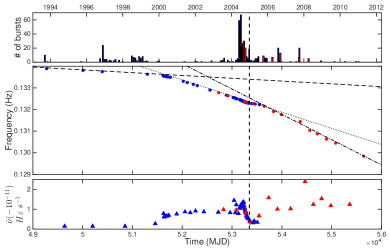
Figure 1.— Frequency and frequency derivative history of SGR 1806$-$20 from mid 1993 until mid 2011. Top panel. Number of bursts (per 30-day intervals). The blue bars represent data collected from Woods et al. (2007) up to 2005 June, and bursts reported in GCNs up to 2012. These represent bursts as seen with wide field-of-view instruments. We also included in red the bursts seen with XMM-Newton. Middle panel. Spin frequency history. Blue dots are collected from Woods et al. (2007) and red dots are our XMM-Newton measurements. The dashed and dotted lines are fits to the frequency derivative from 1993 to 2000 January ($\dot{\nu}=-1.48\times 10^{-12}$ Hz s^-1), and 2001 January to 2004 April ($\dot{\nu}=-8.69\times 10^{-12}$ Hz s^-1, Woods et al. 2007). The dot-dashed line is our best fit to frequency measurements from 2005 July up to the last XMM-Newton observation ($\dot{\nu}=-1.35\times 10^{-11}$ Hz s^-1). Bottom panel. Blue triangles represent instantaneous frequency derivative between two consecutive frequency measurements (excluding XMM-Newton data). Red triangles are the frequency derivative between two consecutive XMM-Newton observations. Note the increase in $\dot{\nu}$ after 2004 and the subsequent decrease around mid 2005. $\dot{\nu}$ remained more or less constant until the last XMM-Newton observation, with some variation around mid 2008.

We first applied a barycenter correction to the filtered pn event files. We then extracted a light curve (LC) for each of the 14 observations in the energy range 1.5$-$10 keV, at the 128-ms and 64-ms resolution for large window and small window mode observations, respectively. We ran the SAS task epiclccorr on these LCs to correct their count rates for background and for the events lost due to various mirror inefficiencies. We performed epoch-folding to derive an initial spin period for each of the observations. Then, we split each observation into 5 smaller intervals, and phase-connected those to achieve a better spin-period measurement and smaller error. The results of this analysis are summarized in Table 1.

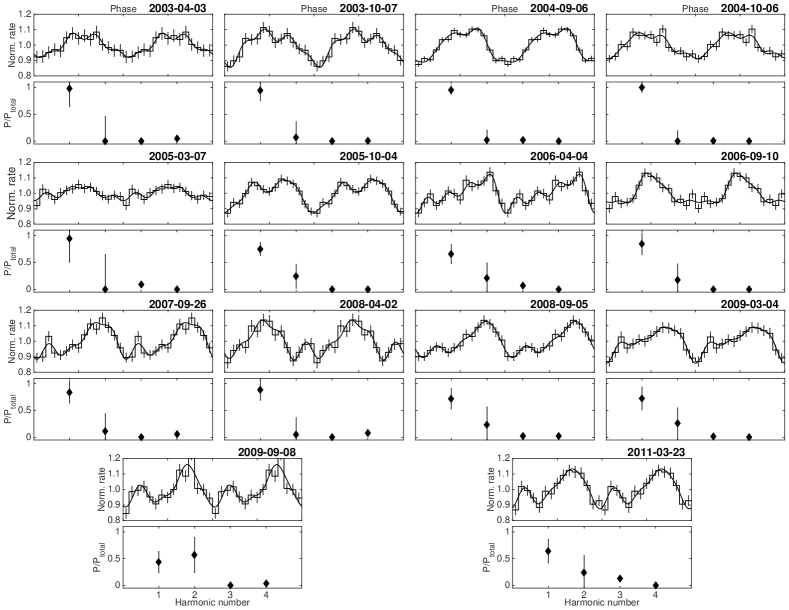
Figure 2.— The background subtracted PPs of all XMM-Newton observations in the 1.5-10 keV, along with their different harmonic contributions. Two cycles are shown for clarity. The pre-GF (prior to 2005) PP has a single broad-peak morphology. It becomes more complex afterwards with contribution from at least the second harmonic. For clarity purposes, we omitted the error bars on the power of harmonics 3 and 4 due to their large uncertainties.

We used our data to extend the work of Woods et al. (2007). In that paper, the authors built a comprehensive frequency and frequency derivative history of SGR 1806$-$20 from late 1993 up to early 2005, a few months after the GF. In Figure 1, we show the timing history of SGR 1806$-$20 extending to the last XMM-Newton observation (red dots), almost six and a half years after the GF. The blue triangles in the bottom panel of Figure 1 show the instantaneous frequency derivative calculated between two adjacent frequency data points, excluding the XMM-Newton data. The red triangles show the frequency derivative as derived from consecutive XMM-Newton observations.

The combined RXTE and XMM-Newton data show some interesting trends; the frequency derivative, almost one year after the GF decreased to the minimum pre-flare value (i.e., maximum spin-down rate; note the negative y-axis values), and remained at that level up to the last XMM-Newton observation. The dashed and dotted lines in Figure 1 are fits to the frequency measurements from 1993 to 2000 January, $\dot{\nu}=-1.48\times 10^{-12}$ Hz s^-1, and 2001 January to 2004 April, $\dot{\nu}=-8.69\times 10^{-12}$ Hz s^-1, respectively (Woods et al. 2007). The dot-dashed line is our best fit to frequency measurements from 2005 July up to the last XMM-Newton observation, $\dot{\nu}=-1.35\times 10^{-11}$ Hz s^-1. This latter $\dot{\nu}$ value is 1.6 times larger than the one observed between 2000 and 2004, and almost an order of magnitude larger than the historical level observed prior to 2000. Deviation from the average after 2005 is seen around 2008 when $\dot{\nu}$ decreased to its lowest value over the course of 8 years (i.e., spin-down rate attained a maximum level), but recovered during the subsequent observation. Unfortunately, the sparse XMM-Newton observations around that time did not allow for detailed modeling of this variation. It is interesting, however, that it happened following a modest bursting episode, as seems to be the case of the gradual change observed in 1999.

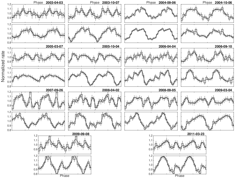
Figure 3.— The background-subtracted PP of all XMM-Newton observations in two energy bands. Two cycles are shown for clarity. The upper rows show the 1.5-4 keV range for each observation and the lower rows show the 4-10 keV range. See text for details.

For completeness, we added in the top panel of Figure 1 the number of bursts detected in each of the XMM-Newton observations (red bars) and the bursts reported in GCNs (Gamma-ray Coordinates Network) from 2005 up to April 2011 (these are mostly bursts identified with the InterPlanetary Network).

Using the spin periods of the different observations, we epoch-folded the data to compute the pulse profiles (PPs) in the 1.5$-$10 keV energy range (Figure 2). We fit the different PPs with a sine plus cosine function (e.g., Bildsten et al. 1997; Younes et al. 2015), including contribution from four harmonics. In Figure 2, we show the power of the different Fourier components relative to the total power in the signal. Similar to the findings of Göǧüş et al. (2002, see also ), we find that the PP prior to the December 2004 GF has a single broad-peak shape with negligible contribution from higher harmonics (Figure 2). During and after the sixth XMM-Newton  observation, i.e., 10 months after the GF, the PP became more complex, with contribution from the second harmonic, indicating a multi-peak structure, clearly seen in the PP (Figure 2).

We then derived the rms pulsed fraction (PF, e.g., Bildsten et al. 1997) of the different observations in the 1.5$-$10 keV energy range, and we estimated its error by simulating 1000 PPs. Despite the changes in PP morphology over the 8 years, we find a steady PF of $\sim$7%. This is consistent with the historical level measured with ASCA and BeppoSAX in 1995. The only change in PF was observed immediately after the GF, when it dropped to a minimum of 3% (observation ID 0164561301, 2005-03-07, see also Rea et al. 2005).

Finally, we looked at the PP morphology in two different energy bands, 1.5$-$4 keV and 4$-$10 keV (Figure 3). The two observations of September and October 2004, when the source flux was at a maximum, showed somewhat similar shapes and PFs in both bands, i.e., a single broad peak. In all other observations, the PPs differed between the two bands (the soft PP was more complex in general than the hard one), and the soft band PF was lower than that of the hard band. However, we note here that due to the low statistics of the data, the soft band rms PFs were not very well constrained and their $3\sigma$ upper limits are consistent with the hard band PFs.

3.2. Spectral analysis

We fit the pn spectra of all 14 observations simultaneously. We started with a simple absorbed PL model and left the PL indices and normalizations free to vary, while we linked the absorption between all spectra. We find an acceptable fit with a $\chi^{2}$ of 5402 for 5284 degrees of freedom (d.o.f.). The hydrogen column density is $N_{\rm H}=(9.7\pm 0.1)\times 10^{22}$ cm^-2. This simple model, however, resulted in strong residuals in the form of a wiggle in the spectrum. We then added a BB component to the model (e.g., Mereghetti et al. 2005). This more complicated spectral shape provided a better fit to the data with a $\chi^{2}$ of 5180 for 5256 d.o.f. According to an F-test, the improvement of the PL+BB model over the single PL has a chance occurrence of $5.3\times 10^{-32}$, hence, we conclude that the addition of the BB is highly significant. The spectra in $\nu{\rm F}_{\nu}$ space, are shown in Figure 4, while the spectral fit results are summarized in Table 2.

Table 2BB and PL spectral parameters

Observation ID	kT	R2,a	$\log F_{\rm BB}$	$\Gamma$	$\log F_{\rm PL}$
	(keV)	(km2)	(erg s-1 cm-2)		(erg s-1 cm-2)
0148210101	$0.6_{-0.2}^{+0.1}$	$1.2_{-0.9}^{+1.4}$	$-11.6_{-0.7}^{+0.3}$	$1.3\pm 0.2$	$-10.70_{-0.07}^{+0.06}$
0148210401	$0.5\pm 0.2$	$3.2_{-2.5}^{+5.7}$	$-11.8\pm 0.6$	$1.4_{-0.2}^{+0.1}$	$-10.63_{-0.06}^{+0.04}$
0205350101	$0.90\pm 0.05$	$0.7\pm 0.2$	$-11.23\pm 0.02$	$1.1\pm 0.1$	$-10.41\pm 0.02$
0164561101	$0.85\pm 0.06$	$0.9\pm 0.3$	$-11.28\pm 0.03$	$1.2\pm 0.1$	$-10.37\pm 0.02$
0164561301	$0.86\pm 0.06$	$1.1_{-0.5}^{+0.4}$	$-11.1\pm 0.2$	$1.0_{-0.3}^{+0.2}$	$-10.55\pm 0.08$
0164561401	$0.77\pm 0.04$	$1.1\pm 0.3$	$-11.34\pm 0.02$	$1.2\pm 0.1$	$-10.68\pm 0.03$
0406600301	$0.75\pm 0.03$	$1.2\pm 0.2$	$-11.28\pm 0.02$	$1.0_{-0.2}^{+0.1}$	$-10.83_{-0.04}^{+0.03}$
0406600401	$0.75\pm 0.08$	$0.5\pm 0.3$	$-11.29\pm 0.02$	$1.5\pm 0.1$	$-10.67\pm 0.03$
0502170301	$0.74\pm 0.04$	$0.9\pm 0.3$	$-11.48\pm 0.03$	$1.4_{-0.2}^{+0.1}$	$-10.83\pm 0.04$
0502170401	$0.69_{-0.04}^{+0.03}$	$1.4\pm 0.3$	$-11.45\pm 0.02$	$1.2\pm 0.2$	$-10.98\pm 0.05$
0554600301	$0.65_{-0.04}^{+0.03}$	$1.3\pm 0.3$	$-11.58\pm 0.03$	$1.4\pm 0.1$	$-10.93_{-0.04}^{+0.03}$
0554600401	$0.63\pm 0.04$	$1.3_{-0.3}^{+0.4}$	$-11.60\pm 0.03$	$1.4\pm 0.1$	$-10.99\pm 0.04$
0604090201	$0.61\pm 0.04$	$1.4_{-0.4}^{+0.5}$	$-11.65\pm 0.03$	$1.5\pm 0.1$	$-10.98\pm 0.04$
0654230401	$0.56\pm 0.04$	$2.0_{-0.5}^{+0.7}$	$-11.64_{-0.03}^{+0.04}$	$1.4\pm 0.1$	$-11.03\pm 0.04$

• ^aDerived by adopting an 8.7 kpc distance (Bibby et al. 2008). Fluxes are in the energy range 0.5-10 keV.

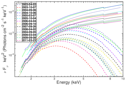
Figure 4.— $\nu F\nu$ best fit model of all XMM-Newton observations. The separate BB and PL components are shown in dashed and dotted lines, respectively. Notice the spectral evolution of the BB component with flux, i.e., the cooling trend with decreasing flux. See text for more details.

Figure 4 shows a clear spectral evolution between the different XMM-Newton observations, in both the PL and the BB components. We plotted the evolution of the different spectral (and temporal) parameters in Figure 5. The BB and PL fluxes increased by a factor of $\sim$2.5 and 4, respectively, compared to their quiescent level, following the onset of the 2004 bursting activity from the source (see panel (a) and, e.g., Mereghetti et al. 2005). This flux increase is clearly accompanied by spectral hardening in both the BB and the PL components (Figure 5).

The spectral parameters decayed back to quiescence levels quasi-exponentially. We fit the PL and the BB fluxes with a model of the form $F(t)\propto\exp^{-t/\tau}$ (black solid lines, panels (f) and (h), Figure 5), where $\tau$ is the characteristic decay time-scale representing a 63% decay of a given parameter back to quiescence. For the PL flux, we find a characteristic decay time-scale of $\tau=441_{-91}^{+104}$ days. The characteristic decay time-scale of the BB flux was much less constrained, with $\tau=990_{-533}^{+509}$ days. We find a similar decay time-scale for the BB temperature, $kT$ (panel (d), Figure 5). A power-law (PL) decay trend, $F(t)\propto t^{\alpha}$ for the above parameters results in a PL decay index $\alpha=-0.65\pm 0.1$ for the PL flux and $-0.4\pm 0.2$ for the BB flux. Finally, we derive the total energy emitted in each component since MJD 53126 (2004 May 01, i.e., the onset of the major bursting activity of 2004) assuming an exponential decay trend, and we find $E_{\rm tot,~{}PL}=3.3\times 10^{43}$ ergs and $E_{\rm tot,~{}BB}=0.7\times 10^{43}$ ergs for the PL and BB components, respectively. We find similar values when using the PL decay trend.

It is worth noting that the BB area increased during the outburst in tandem with the flux decrease from $R^{2}\approx 0.7$ km² to $R^{2}\approx 2.0$ km². Such a behavior has been seen before in a few magnetars (e.g., Woods et al. 2004; Israel et al. 2010). Moreover, the PL to BB flux ratio reached maximum during the beginning of the outburst ($(F_{\rm PL}/F_{\rm BB})\approx 7$), where the PL flux increased by a factor 1.6 more than the BB flux (panel (i), Figure 5). The ratio remained constant after the 2006 observation ($(F_{\rm PL}/F_{\rm BB})\approx 4.5$).

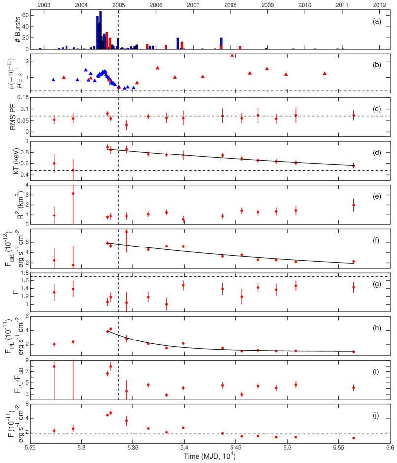
Figure 5.— Temporal and spectral histories of SGR 1806$-$20. Panel (a). Number of bursts in 30 days as seen from wide field-of-view instruments (blue bars), and bursts detected by XMM-Newton (red) bars. Panel (b). Frequency derivative from Woods et al. (2007) (blue triangles), and from XMM-Newton (red triangles). Panel (c). RMS PF. Panel (d). BB temperature, $kT$. Panel (e). BB area, $R^{2}$. Panel (f). BB flux, $F_{\rm BB}$. Panel (g). PL index, $\Gamma$. Panel (h). PL flux, $F_{\rm PL}$. Panel (i). PL to BB flux ratio. Panel (j). Total flux. In all panels, a dotted horizontal line represents the historical level of the given parameter measured with ASCA and/or BeppoSAX. The vertical dashed line is the GF epoch. Solid lines are exponential decay trends for given parameters following the 2004 outburst. See text for details.

Finally, we performed phase-resolved spectroscopy on all observations. We split each observation into 10 equally separated bins in phase space and fit them simultaneously. We linked the absorbing column between the different spectra, and let the BB and PL spectral parameters free to vary. The only clear trend we observe is in the 2004 September and October observations. We find that only the PL flux shows any phase variability (Mereghetti et al. 2005), possibly indicating that the PL component is responsible for most of the pulsed flux. In the remaining cases, unfortunately, the combination of worse statistics compared to the 2004 observations and the very low PF of the source hindered any meaningful conclusions.

4. Discussion

SGR 1806$-$20 is one of the most active magnetars, exhibiting continuous bursting activity, either as strong outbursts like the one detected in 2004, or in sporadic groups of few isolated bursts (Figures 1 and 5, upper panels). SGR 1806$-$20 also shows one of the most erratic behaviors in its timing properties (Figure 1, Woods et al. 2007). The very early observations of the source (Kouveliotou et al. 1998; Woods et al. 2000; Mereghetti et al. 2000) between 1993 and 1999 showed a steady spin-down, $\dot{\nu}=-1.48\times 10^{-12}$ Hz s^-1. From early 1999 to late 2000, the spin-down rate slowly increased to a new steady state, $\dot{\nu}=-8.69\times 10^{-12}$ Hz s^-1, that persisted up to the outburst emitted by the source starting roughly in mid 2004. Thereafter, the source exhibited an erratic behavior leading to another dramatic change in the $\dot{\nu}$ trend (Woods et al. 2007). Our follow-up analysis shows that the spin-down of the source increased again to new long-term average between July 2005 and March 2011 with a new value of $\dot{\nu}=-1.35\times 10^{-11}$ Hz s^-1.

The current SGR 1806$-$20 spin-down rate is an order of magnitude larger than its first historical value. Assuming that the spin-down rate is due to magnetic dipole radiation, the average surface dipole magnetic field strength of a magnetar is $B\approx 3.2\times 10^{19}(\dot{\nu}/\nu^{3})^{1/2}$, where $\nu=1/P$ and $P$ is the spin period of the source. An increase, therefore, of $\dot{\nu}$ by a factor of 10 in a span of 5.5 years would imply an increase of 3.2 in dipole magnetic field strength, which is rather unlikely. We explore below possible mechanisms that may have contributed to the torque increase on the star, hence increasing its spin-down rate.

Thompson et al. (2000, also see ) suggested that persistent luminosity of Alfven waves and particles could generate an additional torque (besides the magnetic dipole one) that would affect the spin-down rate of a magnetar. In this model, continuous low-level seismic activity in a slowly spinning highly-magnetized neutron star will excite magnetospheric Alfven modes and induce a relativistic particle outflow out to a large radius. This particle outflow will import extra torque on the star, increasing its spin-down rate. According to Thompson et al. (2000), the spin-down torque increases by a factor of $\sim(L_{\rm A}/L_{\rm MDR})^{1/2}$, where $L_{\rm A}$ is the persistent luminosity of Alfven waves and particles, and $L_{\rm MDR}$ is the magnetic dipole luminosity (the time-average X-ray output of the SGR in quiescence derived using its dipole field $B$ and spin period, Thompson & Duncan 1996). An order of magnitude increase in spin-down from 2000 to $\sim$mid 2005 would require an increase in the particle luminosity by a factor of 100 over $L_{\rm MDR}$ (considering the latter to correspond to the 2000 early X-ray observations). An obvious effect of such a strong particle output would be a luminous wind nebula (Thompson et al. 2000; Tong et al. 2013, see also Younes et al. 2012). At the 8.7 kpc distance of SGR 1806$-$20, the angular extent of such a wind nebula would be of the order of tens of arcseconds when considering relativistic speeds for the particle outflow, which could possibly be observed with Chandra. Such a wind nebula is, however, not detected in SGR 1806$-$20 (Viganò et al. 2014).

A twisted magnetosphere could also impart excess torque on a magnetar. Magnetic stresses inside the star will cause motion to the footprints of the surface magnetic field lines, causing these external fields to twist (Thompson et al. 2002; Beloborodov 2009). Such a twisted configuration causes a slower decrease in the dipole magnetic field with increasing distance from the neutron star (compared to the case where no twist exists), resulting in a stronger $B$ value at the light cylinder. This excess magnetic energy is then dissipated through an increase in the spin-down rate (Thompson et al. 2002). However, if the affected twisted fields are closed field lines, this temporal variation should also be accompanied by variation in the persistent X-ray spectrum, since a twisted closed field line will have an increase in the optical depth to resonant scattering (Thompson et al. 2002; Beloborodov 2009). On the other hand, if the magnetic flux is dissipated through open field lines, it would affect the torques on the star at large radii without having any effect on the persistent X-ray spectrum (e.g., SGR J1745$-$2900, Kaspi et al. 2014). The spin-down should return to its pure dipole value as the twist angle decreases. The time-scale for the twist energy dissipation could be shorter than the spin period of the source, if the twist is large enough that most of the energy is dissipated through a large magnetic reconnection event, or, more interestingly, for small twist angles, the twist decay time-scale could be as long as a few years (Parfrey et al. 2013, 2012; Beloborodov & Thompson 2007). This model could explain the continuous large spin-down rate of SGR 1806$-$20 up to mid 2011.

We now discuss the long-term spectral evolution of the SGR 1806$-$20 X-ray emission after its 2004 major bursting episode. SGR 1806$-$20, similar to many other magnetar sources, has a 1-10 keV spectrum well fit with the combination of a thermal (BB), and a non-thermal (PL) component. In the magnetar model, the BB component is due to internal heating from the decay of the strong magnetic field, while the non-thermal component is due to resonant cyclotron scattering of these thermal photons by the plasma in the magnetosphere (e.g., Thompson et al. 2002). After the 2004 bursting episode, the flux of the BB and PL increased, while showing spectral hardening (BB temperature increased and PL index, $\Gamma$, decreased). Such a flux-hardness relation is a prediction of the model presented in Thompson et al. (2002) and a very common phenomenon among magnetar sources (e.g., Gavriil & Kaspi 2004; Scholz & Kaspi 2011).

One of the models usually invoked to explain the outburst evolution of a magnetar is of external magnetospheric origin (Beloborodov 2009). In this model, a twist in the magnetosphere, if acting on a bundle of closed field lines, would increase their particle charge density. Returning currents from these field lines would hit their surface footprints, covering a certain area $A$ on the surface, heating it and causing radiation of thermal photons. These thermal photons, in turn, are Compton scattered to higher energies by the plasma in the bundle. As the twist relaxes back to its original untwisted configuration, the bundle disappears gradually, and both the thermal and non-thermal components decrease back to their quiescent level. The relaxation time-scale of the bundle, $t\approx 10^{7}\mu_{32}\Phi_{10}^{-1}A_{11.5}$ s, depends primarily on the footprint size $A_{11.5}=(A/10^{11.5})$ cm², the magnetic dipole moment $\mu_{32}=(\mu/10^{32})$ G cm³, and the electric voltage sustaining its plasma density, $\Phi_{10}=(\Phi/10^{10})$ V (Beloborodov 2009; Mori et al. 2013). Considering a large dipole field $B=10^{15}$ G, a voltage $\Phi=10^{9}$ V, and the area of the BB component $A=4\pi R^{2}$ with $R^{2}\approx 1$ km² (Table 2), one can roughly reconcile the long relaxation time for SGR 1806$-$20, $\sim 10^{8}$ s, with the one predicted by this model. However, the model also predicts that $A$ decreases with decreasing flux, which we do not observe in the data (Figure 5). Moreover, the PL flux increased by a factor of $\sim 1.6$ more than the BB after the onset of the outburst (the 2004 observations), compared to the following observations (after October 2005) where their ratio was more or less constant - a behavior that does not seem to agree with the twisted magnetospheric model.

Heating of the crust from re-arragement of the internal magnetic field, e.g., due to a sudden crack of the crust, is also used to reproduce the relaxation light curve of magnetars (e.g., Lyubarsky et al. 2002; Kouveliotou et al. 2003; Pons & Rea 2012). In this picture, a total energy of the order of $\sim 10^{43}$ ergs is suddenly deposited into the crust, and re-radiated gradually in the form of thermal photons. The total energy emitted from SGR 1806$-$20 throughout the outburst supports these numbers. However, the decay time-scale for such models is expected to be much shorter (of the order of $\sim 100$ days) than the years time-scale we calculate for SGR 1806$-$20 (see discussion in Coti Zelati et al. 2015).

It is remarkable that the PF of SGR 1806$-$20 has remained at a constant value of about 7% from 1994 to 2011 (it only changed for a short period of time immediately after the GF, Rea et al. 2005), while all its other properties changed drastically. This could be an indication that the geometry (and location, e.g., close to the magnetic poles) of the emitting region has remained essentially the same for the last two decades.

Finally, we note that there has been attempts to link the intrinsic properties of magnetars (e.g., $\dot{\nu}$, $B$) with their observed X-ray properties (Marsden & White 2001; Kaspi & Boydstun 2010; An et al. 2012). Such correlations assume that the measured intrinsic properties of these sources outside of bursting episodes are their “true” values (assuming a dipole configuration). It is clear from our analysis of SGR 1806$-$20 (see also Woods et al. 2007) that such assumption is not necessarily correct. The spin-down rate we measure for the late XMM-Newton observations - clearly outside of major bursting episodes - represents an order of magnitude variation in about six years. Hence, the “true” $\dot{\nu}$, and by extrapolation $B$, are currently unknown for SGR 1806$-$20. This could also be true for other magnetars. The above mentioned correlations need to take such possibilities into account.

References

- An et al. (2012) An, H., Kaspi, V. M., Tomsick, J. A., et al. 2012, ApJ, 757, 68
- Archibald et al. (2013) Archibald, R. F., Kaspi, V. M., Ng, C.-Y., et al. 2013, Nature, 497, 591
- Archibald et al. (2015) Archibald, R. F., Kaspi, V. M., Ng, C.-Y., et al. 2015, ApJ, 800, 33
- Arnaud (1996) Arnaud, K. A. 1996, in ASP Conf. Ser. 101: Astronomical Data Analysis Software and Systems V, 17
- Beloborodov (2009) Beloborodov, A. M. 2009, ApJ, 703, 1044
- Beloborodov & Thompson (2007) Beloborodov, A. M. & Thompson, C. 2007, ApJ, 657, 967
- Bibby et al. (2008) Bibby, J. L., Crowther, P. A., Furness, J. P., & Clark, J. S. 2008, MNRAS, 386, L23
- Bildsten et al. (1997) Bildsten, L., Chakrabarty, D., Chiu, J., et al. 1997, ApJS, 113, 367
- Coti Zelati et al. (2015) Coti Zelati, F., Rea, N., Papitto, A., et al. 2015, MNRAS, 449, 2685
- Dib & Kaspi (2014) Dib, R. & Kaspi, V. M. 2014, ApJ, 784, 37
- Dib et al. (2008) Dib, R., Kaspi, V. M., & Gavriil, F. P. 2008, ApJ, 673, 1044
- Esposito et al. (2007) Esposito, P., Mereghetti, S., Tiengo, A., et al. 2007, A&A, 476, 321
- Gaensler et al. (2005) Gaensler, B. M., Kouveliotou, C., Gelfand, J. D., et al. 2005, Nature, 434, 1104
- Gavriil & Kaspi (2004) Gavriil, F. P. & Kaspi, V. M. 2004, ApJ, 609, L67
- Göǧüş et al. (2002) Göǧüş, E., Kouveliotou, C., Woods, P. M., Finger, M. H., & van der Klis, M. 2002, ApJ, 577, 929
- Harding et al. (1999) Harding, A. K., Contopoulos, I., & Kazanas, D. 1999, ApJ, 525, L125
- Hurley et al. (2005) Hurley, K., Boggs, S. E., Smith, D. M., et al. 2005, Nature, 434, 1098
- Israel et al. (2010) Israel, G. L., Esposito, P., Rea, N., et al. 2010, MNRAS, 408, 1387
- Kaspi et al. (2014) Kaspi, V. M., Archibald, R. F., Bhalerao, V., et al. 2014, ApJ, 786, 84
- Kaspi & Boydstun (2010) Kaspi, V. M. & Boydstun, K. 2010, ApJ, 710, L115
- Kaspi et al. (2003) Kaspi, V. M., Gavriil, F. P., Woods, P. M., et al. 2003, ApJ, 588, L93
- Kouveliotou et al. (1998) Kouveliotou, C., Dieters, S., Strohmayer, T., et al. 1998, Nature, 393, 235
- Kouveliotou et al. (2003) Kouveliotou, C., Eichler, D., Woods, P. M., et al. 2003, ApJ, 596, L79
- Lyubarsky et al. (2002) Lyubarsky, Y., Eichler, D., & Thompson, C. 2002, ApJ, 580, L69
- Marsden & White (2001) Marsden, D. & White, N. E. 2001, ApJ, 551, L155
- Mereghetti et al. (2000) Mereghetti, S., Cremonesi, D., Feroci, M., & Tavani, M. 2000, A&A, 361, 240
- Mereghetti et al. (2007) Mereghetti, S., Esposito, P., & Tiengo, A. 2007, Ap&SS, 308, 13
- Mereghetti et al. (2015) Mereghetti, S., Pons, J. A., & Melatos, A. 2015, Space Sci. Rev.
- Mereghetti et al. (2005) Mereghetti, S., Tiengo, A., Esposito, P., et al. 2005, ApJ, 628, 938
- Mori et al. (2013) Mori, K., Gotthelf, E. V., Zhang, S., et al. 2013, ApJ, 770, L23
- Muno et al. (2007) Muno, M. P., Gaensler, B. M., Clark, J. S., et al. 2007, MNRAS, 378, L44
- Ng et al. (2011) Ng, C.-Y., Kaspi, V. M., Dib, R., et al. 2011, ApJ, 729, 131
- Parfrey et al. (2012) Parfrey, K., Beloborodov, A. M., & Hui, L. 2012, ApJ, 754, L12
- Parfrey et al. (2013) Parfrey, K., Beloborodov, A. M., & Hui, L. 2013, ApJ, 774, 92
- Pons & Rea (2012) Pons, J. A. & Rea, N. 2012, ApJ, 750, L6
- Rea & Esposito (2011) Rea, N. & Esposito, P. 2011, in High-Energy Emission from Pulsars and their Systems, ed. D. F. Torres & N. Rea, 247
- Rea et al. (2005) Rea, N., Tiengo, A., Mereghetti, S., et al. 2005, ApJ, 627, L133
- Scholz & Kaspi (2011) Scholz, P. & Kaspi, V. M. 2011, ApJ, 739, 94
- Strüder et al. (2001) Strüder, L., Briel, U., Dennerl, K., et al. 2001, A&A, 365, L18
- Thompson & Blaes (1998) Thompson, C. & Blaes, O. 1998, Phys. Rev. D, 57, 3219
- Thompson & Duncan (1996) Thompson, C. & Duncan, R. C. 1996, ApJ, 473, 322
- Thompson et al. (2000) Thompson, C., Duncan, R. C., Woods, P. M., et al. 2000, ApJ, 543, 340
- Thompson et al. (2002) Thompson, C., Lyutikov, M., & Kulkarni, S. R. 2002, ApJ, 574, 332
- Tiengo et al. (2005) Tiengo, A., Esposito, P., Mereghetti, S., et al. 2005, A&A, 440, L63
- Tong et al. (2013) Tong, H., Xu, R. X., Song, L. M., & Qiao, G. J. 2013, ApJ, 768, 144
- Verner et al. (1996) Verner, D. A., Ferland, G. J., Korista, K. T., & Yakovlev, D. G. 1996, ApJ, 465, 487
- Viganò et al. (2014) Viganò, D., Rea, N., Esposito, P., et al. 2014, Journal of High Energy Astrophysics, 3, 41
- Wilms et al. (2000) Wilms, J., Allen, A., & McCray, R. 2000, ApJ, 542, 914
- Woods et al. (2004) Woods, P. M., Kaspi, V. M., Thompson, C., et al. 2004, ApJ, 605, 378
- Woods et al. (2000) Woods, P. M., Kouveliotou, C., Finger, M. H., et al. 2000, ApJ, 535, L55
- Woods et al. (2007) Woods, P. M., Kouveliotou, C., Finger, M. H., et al. 2007, ApJ, 654, 470
- Woods et al. (2002) Woods, P. M., Kouveliotou, C., Göǧüş, E., et al. 2002, ApJ, 576, 381
- Woods et al. (1999) Woods, P. M., Kouveliotou, C., van Paradijs, J., et al. 1999, ApJ, 524, L55
- Younes et al. (2015) Younes, G., Kouveliotou, C., Grefenstette, B. W., et al. 2015, ApJ, 804, 43
- Younes et al. (2012) Younes, G., Kouveliotou, C., Kargaltsev, O., et al. 2012, ApJ, 757, 39