High degrees in random recursive trees

Abstract.

For $n\geq 1$, let $T_{n}$ be a random recursive tree (RRT) on the vertex set $[n]=\{1,\ldots,n\}$. Let $\deg_{T_{n}}(v)$ be the degree of vertex $v$ in $T_{n}$, that is, the number of children of $v$ in $T_{n}$. Devroye and Lu [6] showed that the maximum degree $\Delta_{n}$ of $T_{n}$ satisfies $\Delta_{n}/\lfloor\log_{2}n\rfloor\to 1$ almost surely; Goh and Schmutz [7] showed distributional convergence of $\Delta_{n}-\lfloor\log_{2}n\rfloor$ along suitable subsequences. In this work we show how a version of Kingman’s coalescent can be used to access much finer properties of the degree distribution in $T_{n}$.

For any $i\in\mathbb{Z}$, let $X_{i}^{(n)}=|\{v\in[n]:\deg_{T_{n}}(v)=\lfloor\log n\rfloor+i\}|$. Also, let $\mathcal{P}$ be a Poisson point process on $\mathbb{R}$ with rate function $\lambda(x)=2^{-x}\cdot\ln 2$. We show that, up to lattice effects, the vectors $(X_{i}^{(n)},\,i\in\mathbb{Z})$ converge weakly in distribution to $(\mathcal{P}[i,i+1),\,i\in\mathbb{Z})$. We also prove asymptotic normality of $X_{i}^{(n)}$ when $i=i(n)\to-\infty$ slowly, and obtain precise asymptotics for ${\mathbf{P}}\left(\Delta_{n}-\log_{2}n>i\right)$ when $i(n)\to\infty$ and $i(n)/\log n$ is not too large. Our results recover and extends the previous distributional convergence results on maximal and near-maximal degrees in random recursive trees.

1. Statement of results

The process of random recursive trees $(T_{n},\,n\geq 1)$ is defined as follows. $T_{1}$ has a single node with label 1, which its root. The tree $T_{n+1}$ is obtained from $T_{n}$ by directing an edge from a new vertex $n+1$ to $v\in[n]$; the choice of $v$ is uniformly random and independent for each $n\in\mathbb{N}$. We call $T_{n}$ a random recursive tree (RRT) of size $n$.

As a consequence of the construction, vertex-labels in $T_{n}$ increase along root-to-leaf paths. Rooted labelled trees with such property are called increasing trees. It is not difficult to see that, in fact, $T_{n}$ is uniformly chosen among the set $\mathcal{I}_{n}$ of increasing trees with vertex set $[n]$.

We write $\deg_{T_{n}}(v)$ to denote the number of children of $v$ in $T_{n}$. The degree distribution of $T_{n}$ is encoded by the variables $Z_{i}^{(n)}=|\{v\in[n]:\deg_{T_{n}}(v)=i\}|$, for $i\geq 0$. In fact, the study of RRT’s started with a paper by Na and Rapoport [13] in which they obtained, for any fixed $i\geq 0$, the convergence $\mathbb{E}(Z_{i}^{(n)})/n\to 2^{-i-1}$ as $n\to\infty$; this result was extended to convergence in probability by Meir and Moon in [12]. Mahmoud and Smythe [11] derived the asymptotic joint normality of $Z_{i}^{(n)}$ for $i\in\{0,1,2\}$; and finally, Janson [8] extended the joint normality to $Z_{i}^{(n)}$ for $i\geq 0$ and gave explicit formulae for the covariance matrix.

The above results concern typical degrees; the focus in this work is large degree vertices, and in particular the maximum degree in $T_{n}$, which we denote $\Delta_{n}=\max_{v\in[n]}\deg_{T_{n}}(v)$. For the rest of the paper we write $\log$ to denote logarithms with base 2, and $\ln$ to denote natural logarithms. For $n\in\mathbb{N}$ let $\varepsilon_{n}=\log n-\lfloor\log n\rfloor$.

A heuristic to find the order of $\Delta_{n}$ is that, if $\mathbb{E}(Z_{i}^{(n)})\approx n2^{-i-1}$ were to hold for all $i$, as it does when $i$ is fixed, then we would have $\mathbb{E}(Z_{\lfloor\log n\rfloor}^{(n)})\approx n2^{-\lfloor\log n\rfloor-1}=2^{-1+\varepsilon_{n}}$. This heuristic suggests that $\Delta_{n}$ is of order $\log n$. This is indeed the case: Szymanski [15] proved that ${\mathbf{E}}\left[\Delta_{n}\right]/\log n\to 1$ as $n\to\infty$, and Devroye and Lu [6] later established that $\Delta_{n}/\log n\to 1$ a.s.. Finally, Goh and Schmutz [7] showed that $\Delta_{n}-\lfloor\log n\rfloor$ converges in distribution along suitable subsequences, and identified the possible limiting laws.

Since we focus on maximal degrees, it is useful to let

$$X_{i}^{(n)}=Z_{i+\lfloor\log n\rfloor}^{(n)}=|\{v\in[n]:\deg_{T_{n}}(v)=\lfloor\log n\rfloor+i\}|,$$

for $n\in\mathbb{N}$ and $i\geq-\lfloor\log n\rfloor$. The following is a simplified version of one of our main results.

Theorem 1.1.

Fix $\varepsilon\in[0,1]$. Let $(n_{l})_{l\geq 1}$ be an increasing sequence of integers satisfying $\varepsilon_{n_{l}}\to\varepsilon$ as $l\to\infty$. Then, as $l\to\infty$

$$(X_{i}^{(n_{l})},\,i\in\mathbb{Z})\stackrel{{\scriptstyle\mathrm{d}}}{{\longrightarrow}}(P^{\varepsilon}_{i},\,i\in\mathbb{Z})$$

jointly for all $i\in\mathbb{Z}$ where the $P^{\varepsilon}_{i}$ are independent Poisson r.v.’s with mean $2^{-i-1+\varepsilon}$.

The random variables $X_{i}^{(n)}$ do not converge in distribution as $n\to\infty$ without taking subsequences; this is essentially a lattice effect caused by the floor $\lfloor\log n\rfloor$ in the definition of $X^{(n)}_{i}$.

Theorem 1.1 can be stated in terms of weak convergence of point processes (which is equivalent to convergence of finite dimensional distributions (FDD’s); see Theorem 11.1.VII in [4]). In fact, we will also prove convergence (along subsequences) of

$$X_{\geq i}^{(n)}=\sum_{k\geq i}X_{k}^{(n)}=|\{v\in[n]:\deg_{T_{n}}(v)\geq\lfloor\log n\rfloor+i\}|.$$

This is useful as it yields information about $\Delta_{n}$ which cannot be derived from Theorem 1.1. We formulate this result as a statement about convergence of point processes, and now provide the relevant definitions. Let $\mathbb{Z}^{*}=\mathbb{Z}\cup\{\infty\}$. Endow $\mathbb{Z}^{*}$ with the metric defined by $\mathrm{d}(i,j)=|2^{-j}-2^{-i}|$ and $\mathrm{d}(i,\infty)=2^{-i}$ for $i,j\in\mathbb{Z}$. Let $\mathcal{M}_{\mathbb{Z}^{*}}^{\#}$ be the space of boundedly finite measures of $\mathbb{Z}^{*}$.

Let $\mathcal{P}$ be a Poisson point process on $\mathbb{R}$ with rate function $\lambda(x)=2^{-x}\cdot\ln 2$. For each $\varepsilon\in[0,1]$ let $\mathcal{P}^{\varepsilon}$ be the point process on $\mathbb{Z}^{*}$ given by

$$\mathcal{P}^{\varepsilon}=\sum_{x\in\mathcal{P}}\delta_{\lfloor x+\varepsilon\rfloor}.$$

Similarly, for all $n\in\mathbb{N}$ let

$$\mathcal{P}^{(n)}=\sum_{v\in[n]}\delta_{\deg_{T_{n}}(v)-\lfloor\log n\rfloor}.$$

Then, for each $i\in\mathbb{Z}$ we have that

$$\mathcal{P}^{\varepsilon}(\{i\}):=|\{x\in\mathcal{P}:\lfloor x+\varepsilon\rfloor=i\}|=|\{x\in\mathcal{P}:x\in[i-\varepsilon,i+1-\varepsilon)\}|$$

has distribution $\mathrm{Poi}(2^{-i-1+\varepsilon})$; also $\mathcal{P}^{(n)}(\{i\})=X_{i}^{(n)}$. We abuse notation by writing, e.g., $\mathcal{P}^{(n)}(i)=\mathcal{P}^{(n)}(\{i\})$.

It is clear that $\mathcal{P}^{(n)}$ and $\mathcal{P}^{\varepsilon}$ are elements of $\mathcal{M}_{\mathbb{Z}^{*}}^{\#}$. The advantage of working on the state space to $\mathbb{Z}^{*}$ is that intervals $[k,\infty]$ are compact. In particular, the convergence of FDD’s of $\mathcal{P}^{(n_{l})}$ implies the convergence in distribution of $X_{\geq i}^{(n_{l})}=\mathcal{P}^{(n_{l})}[i,\infty)$.

Theorem 1.2.

Fix $\varepsilon\in[0,1]$. Let $(n_{l})_{l\geq 1}$ be an increasing sequence of integers satisfying $\varepsilon_{n_{l}}\to\varepsilon$ as $l\to\infty$. Then in $\mathcal{M}_{\mathbb{Z}^{*}}^{\#}$, $\mathcal{P}^{(n_{l})}$ converges weakly to $\mathcal{P}^{\varepsilon}$ as $l\to\infty$. Equivalently, for any $i<i^{\prime}\in\mathbb{Z}$, jointly as $l\to\infty$

$$(X_{i}^{(n_{l})},\ldots,X_{i^{\prime}-1}^{(n_{l})},X_{\geq i}^{(n_{l})})\stackrel{{\scriptstyle\mathrm{d}}}{{\longrightarrow}}(\mathcal{P}^{\varepsilon}(i),\ldots,\mathcal{P}^{\varepsilon}(i^{\prime}-1),\mathcal{P}^{\varepsilon}[i^{\prime},\infty)).$$

Note that Theorem 1.1 follows from Theorem 1.2. We finish this section stating two additional results. The first is an extension of the main theorem from [7], that result being essentially the case $i=O(1)$.

Theorem 1.3.

For any $i=i(n)$ with $i+\log n<2\ln n$ and $\liminf_{n\to\infty}i(n)>-\infty$,

$$\mathbf{P}(\Delta_{n}\geq\lfloor\log n\rfloor+i)=(1-\exp\{-2^{-i+\varepsilon_{n}}\})(1+o(1)).$$

When $i=O(1)$, the assertion of Theorem 1.3 is a straight-forward consequence of Theorem 1.2. For the case that $i(n)\to\infty$ we use estimates for the first and second moments of $X_{\geq i}^{(n)}$; note that $\{\Delta_{n}<\lfloor\log n\rfloor+i\}=\{X_{\geq i}^{(n)}=0\}$.

Finally, we also obtain the asymptotic normality for $X_{i}^{(n)}$ when $i$ tends to $-\infty$ slowly enough.

Theorem 1.4.

If $i=i(n)\to-\infty$ and $i=o(\ln n)$, then as $n\to\infty$

$$\frac{X_{i}^{(n)}-2^{-i-1+\varepsilon_{n}}}{\sqrt{2^{-i-1+\varepsilon_{n}}}}\stackrel{{\scriptstyle\mathrm{d}}}{{\to}}N(0,1).$$

Remark 1.5.

Up to lattice effects, Theorems 1.2 and 1.4 extend the range of $i=i(n)$ for which the heuristic that $Z_{i}^{(n)}\approx n2^{-i-1}$ holds.

A key novelty of our approach is that for each $n$ we use Kingman’s coalescent to generate a tree $T^{(n)}$ whose vertex degrees $\{\deg_{T^{(n)}}(v)\}_{v\in[n]}$ are exchangeable but otherwise have the same law as degrees in $T_{n}$. (See [2], Chapter 2 for a description of Kingman’s coalescent, and [1], Section 2.2 for a description of the connection with random recursive trees which we exploit in this paper.) By this we mean that if $\sigma:[n]\to[n]$ is a uniformly random permutation then the following distributional identiy holds:

(1) $$(\deg_{T^{(n)}}(v),\,v\in[n])\stackrel{{\scriptstyle\mathrm{d}}}{{=}}(\deg_{T_{n}}(\sigma(v)),\,v\in[n]).$$

We describe the trees $T^{(n)}$, $n\in\mathbb{N}$ in Section 3.

An essentially equivalent construction was used by Devroye [5] to study union-find trees. In [14], Pittel related the results of [5] on union-find trees to the height of RRT’s. It is worth mentioning that both Kingman’s coalescent and the union-find trees can be equivalently represented as binary trees or, as we will see in Section 3, as RRT’s. Aside from the works [5] and [14], it seems that the use of Kingman’s coalescent or of union-find trees to study RRT’s is rare. However, it turns out to provide just the right perspective for studying high degree vertices.

2. Outline

In this section we sketch the approach used in the paper. The proofs of the theorems relay on the computation of the moments of the FDD’s of $\mathcal{P}^{(n)}$; these estimates are given in Proposition 2.1. In particular, the proofs of Theorems 1.2 and 1.4 use the method of moments (e.g., see [9] Section 6.1, and [3] Section 1.5).

Any FDD of $\mathcal{P}^{(n)}$ can be recovered from suitable marginals of the joint distribution of $(X_{i}^{(n_{l})},\ldots,X_{i^{\prime}-1}^{(n_{l})},X_{\geq i^{\prime}}^{(n_{l})})$ for some $i<i^{\prime}\in\mathbb{Z}$. For simplicity, we focus for the moment on collections of variables $X_{i}^{(n)},\ldots,X_{i^{\prime}}^{(n)}$ for $i\leq i^{\prime}$. For $r\in\mathbb{R}$ and $a\in\mathbb{N}$ write $(r)_{a}=r(r-1)\cdots(r-a+1)$, also let $(r)_{0}=1$. We will prove that for any non-negative integers $a_{i},\ldots,a_{i^{\prime}}$, as $n\to\infty$, we have

(2) $${\mathbf{E}}\left[\prod_{i\leq k\leq i^{\prime}}(X_{k}^{(n)})_{a_{k}}\right]-\prod_{i\leq k\leq i^{\prime}}\left(2^{-(k+1)+\varepsilon_{n}}\right)^{a_{k}}\to 0.$$

This immediately yields Theorem 1.1.

By the linearity of expectation, proving (2) reduces to understanding the probabilities

(3) $${\mathbf{P}}\left(\deg_{T_{n}}(v_{k})=\lfloor\log n\rfloor+i_{k},\,k\in[K]\right)$$

for all $i_{1},\ldots i_{K}\in\mathbb{N}$ and $v_{1},\ldots v_{K}\in[n]$, $K\in\mathbb{N}$; see Section 5 for more details.

In the standard model for RRT’s described at the beginning, $\deg_{T_{n}}(v)$ is a sum of Bernoulli variables:

$$\deg_{T_{n}}(v)=\sum_{v<u\leq n}\mathbf{1}_{\{u\to v\}}.$$

The lack of symmetry of the degrees $\{\deg_{T_{n}}(v)\}_{v\in[n]}$ complicates the analysis of (3). In proving that $\Delta_{n}/\log n\stackrel{{\scriptstyle\mathrm{a.s.}}}{{\rightarrow}}1$, Devroye and Lu [6] used that $\{\deg_{T_{n}}(v)\}_{v\in[n]}$ are negatively orthant dependent (see [10] for a definition), which in particular means that for all $S\subset[n]$ and $m_{1},\ldots,m_{n}\in\mathbb{N}$

(4) $${\mathbf{P}}\left(\deg_{T_{n}}(v)\geq m_{v},\,v\in S\right)\leq\prod_{v\in S}{\mathbf{P}}\left(\deg_{T_{n}}(v)\geq m_{v}\right)$$

and then obtained upper bounds for ${\mathbf{P}}\left(deg_{T_{n}}(v)\geq c\ln n\right)$ for each $v\in[n]$.

One approach to studying high degrees in $T_{n}$ would be to obtain matching lower bounds for ${\mathbf{P}}\left(\deg_{T_{n}}(v)\geq m_{v},\,v\in S\right)$, with uniform error terms even when $m_{v}$ is large. Instead, we study trees $T^{(n)}$, mentioned in (1), above, for which we can obtain precise asymptotics for the analogous probabilities

(5) $${\mathbf{P}}\left(\deg_{T^{(n)}}(v)\geq m_{v},\,v\in[K]\right).$$

The core of the paper lies in Proposition 4.2, which gives precise estimates of (5) for $m_{1},\ldots,m_{K}$ in a suitable range. Broadly speaking, $\deg_{T^{(n)}}(v)$ depends on a set of random selection times ${\mathcal{S}}_{v}$ and the first streak of heads in a sequence of $|{\mathcal{S}}_{v}|$ fair coin flips. As mentioned in the previous section, the degrees of $T^{(n)}$ have the same distribution as the degrees in $T_{n}$. Consequently, our estimation of (5) allows us to obtain the following moments estimate.

Proposition 2.1.

For all $c\in(0,2)$ and $K\in\mathbb{N}$ there is $\alpha=\alpha(c,K)>0$ such that the following holds. Fix any integers $i,i^{\prime}$ with $0<i+\log_{n}<i^{\prime}+\log_{n}<c\ln n$. Then for any non-negative integers $a_{i},\ldots,a_{i^{\prime}}$ with $a_{i}+\ldots+a_{i^{\prime}}=K$, we have

$${\mathbf{E}}\left[(X_{\geq i^{\prime}}^{(n)})_{a_{i^{\prime}}}\prod_{i\leq k<i^{\prime}}(X_{k}^{(n)})_{a_{k}}\right] =\left(2^{-i^{\prime}+\varepsilon_{n}}\right)^{a_{i^{\prime}}}\prod_{i\leq k<i^{\prime}}\left(2^{-(k+1)+\varepsilon_{n}}\right)^{a_{k}}(1+o(n^{-\alpha})).$$

Equipped with Proposition 2.1, the proofs of the theorems are straightforward. The rest of the paper is organized as follows. In Section 3, we explain how to define the trees $T^{(n)}$ using Kingman’s coalescent and establish the distributional relation between $T^{(n)}$ and the RRT; see Corollary 3.4. In Section 4, we define the random sets $({\mathcal{S}}_{v},v\in T^{(n)})$ and explain their relation with degrees in $T^{(n)}$. The proof of Proposition 4.2, which is our estimate of (5), is then presented using a decoupling of the events in (5) and the concentration of the random variables $|{\mathcal{S}}_{v}|$. Finally, the proof of Proposition 2.1 is given in Section 5 and the proof of Theorems 1.2-1.4 are in Section 6.

3. Random Recursive Trees and Kingman’s coalescent

In this section we give a representation of Kingman’s coalescent in terms of labelled forests, and relate it to RRT’s. All trees in the remainder of the paper are rooted, and we write $r(t)$ for the root of tree $t$. By convention, edges of a tree are directed towards the root of the tree and we write $uv$ to denote an edge directed from $u$ to $v$. A forest $f$ is a set of trees whose vertex sets are pairwise disjoint. The vertex set of a forest, denoted $V(f)$, is the union of the vertex sets of its trees. Similarly, $E(f)$ denotes the set of edges in the trees of $f$. For $n\geq 1$, let

$$\mathcal{F}_{n}=\{f:V(f)=[n]\}$$

be the set of forests with vertex set $[n]$.

A sequence $C=(f_{1},\ldots,f_{n})$ of elements of $\mathcal{F}_{n}$ is an $n$-chain if $f_{1}$ is the forest in $\mathcal{F}_{n}$ with $n$ one-vertex trees and, for $1\leq i<n$, $f_{i+1}$ is obtained from $f_{i}$ by adding a directed edge between the roots of some pair of trees in $f_{i}$. If $(f_{1},\ldots,f_{n})$ is an $n$-chain then for $1\leq i\leq n$, the forest $f_{i}$ consists of $n+1-i$ trees, and in this case we list its elements in increasing order of their smallest-labelled vertex as $t_{1}^{(i)},\ldots,t_{n+1-i}^{(i)}$.

Definition 3.1.

Kingman’s $n$-coalescent is the random $n$-chain $\mathbf{C}=(F_{1},\ldots,F_{n})$ built as follows. Independently for each $1\leq i\leq n-1$ let $\{a_{i},b_{i}\}$ be a random pair uniformly chosen from $\{\{a,b\}:1\leq a<b\leq n+1-i\}$ and let $\xi_{i}$ be independent with $\mathrm{Bernoulli}(1/2)$ distribution.

For $1\leq i<n$, construct $F_{i+1}$ from $F_{i}$ as follows. If $\xi_{i}=1$ then add an edge from $r(T_{b_{i}}^{(i)})$ to $r(T_{a_{i}}^{(i)})$ and if $\xi_{i}=0$ then add an edge from $r(T_{a_{i}}^{(i)})$ to $r(T_{b_{i}}^{(i)})$. The forest $F_{i+1}$ consists of the new tree and the remaining $n-1-i$ unaltered trees from $F_{i}$.

For an example of the process see Figure 1.

Figure 1. An example of Kingman’s $n$-coalescent $\mathbf{C}=(F_{1},\ldots,F_{n})$ for $n=6$. For $1\leq i<n$, $F_{i}$ has, in dotted line, the edge in $E(F_{i+1})\setminus E(F_{i})$. Edges are marked with their time of addition; this is the function $L^{-}_{\mathbf{C}}$ defined after Lemma 3.2. In this instance, $\xi_{1}=\xi_{3}=\xi_{4}=1$, $\xi_{2}=\xi_{5}=0$ and $\{a_{1},b_{1}\}=\{2,5\},$ $\;\{a_{2},b_{2}\}=\{1,5\},\;\{a_{3},b_{3}\}=\{1,4\},\;\{a_{4},b_{4}\}=\{2,3\},\;\{a_{5},b_{5}\}=\{1,2\}$.

Lemma 3.2.

Let $\mathcal{CF}_{n}$ be the set of $n$-chains of elements in $\mathcal{F}_{n}$. Then $|\mathcal{CF}_{n}|=n!(n-1)!$ and Kingman’s $n$-coalescent is a uniformly random element of $\mathcal{CF}_{n}$.

Proof.

Fix an $n$-chain $(f_{1},\ldots,f_{n})\in\mathcal{CF}_{n}$. Then

$${\mathbf{P}}\left((F_{1},\ldots,F_{n})=(f_{1},\ldots,f_{n})\right)=\prod_{k=1}^{n-1}{\mathbf{P}}\left(F_{k+1}=f_{k+1}|F_{j}=f_{j},\,1\leq j\leq k\right).$$

Among the $(n+1-k)(n-k)$ possible oriented edges between roots of $f_{k}$, there is exactly one whose addition yields $f_{k+1}$. It follows that the $k$-th term in the above product is $\left((n+1-k)(n-k)\right)^{-1}$, so ${\mathbf{P}}\left((F_{1},\ldots,F_{n})=(f_{1},\ldots,f_{n})\right)=\left[n!(n-1)!\right]^{-1}$. The result follows since this expression does not depend on $(f_{1},\ldots,f_{n})\in\mathcal{CF}_{n}$. ∎

Recall that $\mathcal{I}_{n}$ is the set of increasing trees with vertex set $[n]$. It is not difficult to see that $|\mathcal{I}_{n}|=(n-1)!$ and that a RRT is a uniformly random element of $\mathcal{I}_{n}$.

There is a natural mapping $\phi$ between $n$-chains and increasing trees. Given an $n$-chain $C=(f_{1},\ldots,f_{n})$, write $t^{(n)}:=t_{1}^{(n)}$ for the unique tree in $f_{n}$. Let $L^{-}_{C}:E(t^{(n)})\to[n-1]$ be defined as follows. For each $e\in E(t^{(n)})$, let

$$L^{-}_{C}(e)=\max\{i\in[n-1]:\,e\notin E(t^{(i)})\}.$$

We think of $L^{-}_{C}$ as a function that keeps track of the time of addition of the edges along the $n$-chain $C$. Now, we define a vertex labelling $L_{C}:V(t^{(n)})\to[n]$ as follows. Let $L_{C}(r(t^{(n)}))=1$ and for each $uv\in E(t^{(n)})$, let

$$L_{C}(u)=n+1-L^{-}_{C}(uv);$$

then $L_{C}(u)$ is the number of trees in the forest just before $uv$ is added.

Note that for each $i\in[n-1]$, the new edge in $f_{i+1}$ joins the roots of two trees in $f_{i}$ and is directed towards the root of the resulting tree. Thus, the labels $\{L^{-}_{C}(e),\,e\in E(t^{(n)})\}$ increase along all paths in $t^{(n)}$ towards the root $r(t^{(n)})$ and consequently, the labels $\{L_{C}(v),\,v\in V(t^{(n)})\}$ increase along root-to-leaf paths in $t^{(n)}$. This shows that relabelling the vertices of $t^{(n)}$ with $L_{C}$ yields an increasing tree (specifically, an element of $\mathcal{I}_{n}$). See Figure 2 for an example.

Figure 2. On the left a tree $t^{(n)}$; edges are marked with $L^{-}_{C}$, from which the $n$-chain $C=(f_{1},\ldots,f_{n})$ can be recovered. On the right, the increasing tree $\phi(f_{1},\ldots,f_{n})$; it has the shape of $t^{(n)}$ and the vertex labels $\{L_{C}(v),\,v\in V(t^{(n)})\}$.

Proposition 3.3.

Let $\phi:\mathcal{CF}\to\mathcal{I}_{n}$ be defined as follows. For an $n$-chain $C=(f_{1},\ldots,f_{n})$ let $\phi(C)$ be the tree obtained from $t^{(n)}$ by relabelling its vertices with $L_{C}$. Then $\phi(\mathbf{C})$, the push-forward of Kingman’s $n$-coalescent by $\phi$, has the law of a RRT of size $n$.

Proof.

First, we prove that $\phi$ is onto. Fix an increasing tree $t\in\mathcal{I}_{n}$. For each $j\in V(t)\setminus\{1\}$, let $v_{j}\in V(t)$ be such that $jv_{j}\in E(t)$, recall that edges are directed toward the root of $t$, thus $v_{j}$ is uniquely defined. For each $1<j\leq n$, let $e_{n-j+1}=ju_{j}$.

Now construct an $n$-chain $C$ as follows. Let $f_{1}$ be the forest with $n$ one-vertex trees. For each $1<i\leq n$ construct $f_{i}$ from $f_{i-1}$ by adding the edge $e_{i-1}$. In other words, for each $1\leq i<n$, $L^{-}_{C}(e_{i})=i$ and so $L_{C}(n+1-i)=n+1-L^{-}_{C}(e_{i})=n+1-i$; also since $r(t)=1$, we have $L_{C}(1)=1$. Consequently, $\phi(C)=t$.

We claim that $|\phi^{-1}(t)|\geq n!$ for any $t\in\mathcal{I}_{n}$. To see this, consider an $n$-chain $C$ and a permutation $\sigma:[n]\to[n]$. Let $C_{\sigma}$ be the $n$-chain obtained from $C$ by permuting the vertices in each forest of $C$ by $\sigma$. Since $L_{C}(v)$ depends only on the time of addition of its outgoing edge (if any), it follows that $\phi(C)=\phi(C_{\sigma})$ for all permutations $\sigma$. By Lemma 3.2, this shows that $\phi$ is $n!$-to-1 and that $\phi(\mathbf{C})$ is a uniform element in $\mathcal{I}_{n}$. ∎

Since $\phi(\mathbf{C})$ preserves the shape of $T^{(n)}$ and only relabels its vertices, the degrees in $T^{(n)}$ and $\phi(\mathbf{C})$ are equal as multisets: $\{deg_{T^{(n)}}(v)\}_{v\in[n]}=\{deg_{\phi(\mathbf{C})}(v)\}_{v\in[n]}$. This immediately gives the following key corollary of Proposition 3.3, on which the rest of the paper relies.

Corollary 3.4.

For all $n\in\mathbb{N}$, we have the following equality in distribution holds jointly for all $i\in\mathbb{Z}$,

$$X_{i}^{(n)}\stackrel{{\scriptstyle\mathrm{d}}}{{=}}|\{v\in[n]:\deg_{T^{(n)}}(v)=\lfloor\log n\rfloor+i\}|.$$

We now proceed to the study of the joint distribution of the vertex degrees in $T^{(n)}$.

4. Degree distribution: Selection sets and coin flips

By construction, the vertex degrees $\{\deg_{T^{(n)}}(v)\}_{v\in[n]}$ are exchangeable. Our next goal is to explain how to approximate (5); that is, for any fixed $k\in\mathbb{N}$ and integers $m_{1},\ldots,m_{k}<2\ln n$, to obtain estimates for ${\mathbf{P}}\left(\deg_{T^{(n)}}(v)\geq m_{v},\,v\in[k]\right)$.

The key to analyse the degrees in $T^{(n)}$ is to understand how the degrees of a vertex $v\in[n]$ change in Kingman’s coalescent $\mathbf{C}=(F_{1},\ldots,F_{n})$. For any vertex $v$ and $1\leq i\leq n$, denote $\deg_{F_{i}}(v)$ the number of children of $v$ in $F_{i}$. Also, we will simply write $\deg(v)=\deg_{F_{n}}(v)=\deg_{T^{(n)}}(v)$. For each $1\leq i<n$, if $\xi_{i}=1$ we say that $\xi_{i}$ favours the vertices of $T_{a_{i}}^{(i)}$, and otherwise that it favours the vertices of $T_{b_{i}}^{(i)}$. For $v\in[n]$, let

$${\mathcal{S}}_{v}=\{i\in[n-1]:v\in T_{a_{i}}^{(i)}\cup T_{b_{i}}^{(i)}\}.$$

For any vertex $v$, and $1\leq i<n$, $\deg_{F_{i+1}}(v)$ increases by one only if $v$ is a root in $F_{i}$, $i\in{\mathcal{S}}_{v}$ and $\xi_{i}$ favours $v$; see Figure 3. Conversely, let $p_{v}=\min\{i\in{\mathcal{S}}_{v},\,\xi_{i}\text{ does not favour }v\}$, then the first $F_{i+1}$ in which $v$ is not a root is exactly $i=p_{v}$. In this case, in $F_{p_{v}+1}$ there is an outgoing edge from $v$, and $v$ is not a root of any subsequent forests. As a consequence, $\deg_{F_{j}}(v)=\deg_{F_{p_{v}}}(v)$ for $p_{v}<j\leq n$.

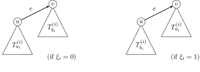
Figure 3. If $v$ is a root in $T_{a_{i}}^{(i)}\cup T_{b_{i}}^{(i)}$ and $\xi_{i}$ favours $v$, then $v$ increases its degree and remains a root in $F_{i+1}$.

Fact 4.1.

For $v\in[n]$, $\deg(v)=\deg_{F_{p_{v}}}(v)=|{\mathcal{S}}_{v}\cap[p_{v}-1]|$.

In other words, $\deg(v)$ depends only on its first streak of favourable random variables $\xi_{i}$ with $i\in{\mathcal{S}}_{v}$. More precisely, given $|{\mathcal{S}}_{v}|$, the degree $\deg(v)$ is distributed as $\min\{|{\mathcal{S}}_{v}|,G\}$, where $G$ is a $\mathrm{Geometric}(1/2)$ r.v. independent of ${\mathcal{S}}_{v}$.

Thus, it is relevant to observe that $|{\mathcal{S}}_{v}|$ is distributed as an sum of independent (though not identically distributed) Bernoulli random variables and so it is concentrated around its mean ${\mathbf{E}}\left[|{\mathcal{S}}_{v}|\right]=2\ln n+O(1)$; a more precise statement can be found in Proposition 4.5 below. Since $|{\mathcal{S}}_{v}|\to\infty$ in probability as $n\to\infty$, it follows easily that $\deg(v)$ is asymptotically geometric for any fixed node $v$. More strongly, the following proposition shows that for any fixed $k$, the random variables $\{\deg_{T^{(n)}}(v)\}_{v\in[k]}$ asymptotically behave like independent Geometric random variables, even if they are conditioned to be quite large.

Proposition 4.2.

Fix $c\in(0,2)$ and $k\in\mathbb{N}$. There exists $\alpha=\alpha(c,k)>0$ such that uniformly over positive integers $m_{1},\ldots,m_{k}<c\ln n$,

$${\mathbf{P}}\left(\deg_{T^{(n)}}(v)\geq m_{v},\,v\in[k]\right)=2^{-\sum_{v}m_{v}}(1+o(n^{-\alpha})).$$

We now explain how the events in the proposition above can be decoupled into a product of two probabilities, one of them corresponding to tail bounds for the random variables $|{\mathcal{S}}_{v}|$. We start with an upper bound for Proposition 4.2.

Lemma 4.3.

For any $k\in\mathbb{N}$ and positive integers $m_{1},\ldots,m_{k}<n$,

$${\mathbf{P}}\left(\deg(v)\geq m_{v},\,v\in[k]\right)\leq 2^{-\sum_{v}m_{v}}\,{\mathbf{P}}\left(|{\mathcal{S}}_{v}|\geq m_{v},\,v\in[k]\right).$$

Equality holds for $k=1$.

Proof.

For each $v\in[k]$ list ${\mathcal{S}}_{v}$ in increasing order as $(i_{v,j},\,1\leq j\leq|{\mathcal{S}}_{v}|)$. Let $\mathcal{A}$ be the set of sequences $A=(A_{1},\ldots,A_{k})$ satisfying $A_{v}\subset[n-1]$ and $|A_{v}|=m_{v}$ for all $v\in[k]$. For every $A\in\mathcal{A}$, let $D_{A}$ be the event that $|{\mathcal{S}}_{v}|\geq m_{v}$ and $\{i_{v,1},\ldots,i_{v,m_{v}}\}=A_{v}$, for all $v\in[k]$. By Fact 4.1, if $\deg(v)\geq m_{v}$ then necessarily $|{\mathcal{S}}_{v}|\geq m_{v}$ so

$$\{\deg(v)\geq m_{v},\,v\in[k]\}\cap D_{A}=\{\xi_{i_{v,j}}\text{ favours $v$ for all }j\in[m_{v}],\,v\in[k]\}\cap D_{A}.$$

Now, $\xi_{i}$ are i.i.d Bernoulli(1/2) r.v.’s. Thus, if $D_{A}$ has positive probability then

$${\mathbf{P}}\left(\xi_{i_{v,j}}\text{ favours $v$ for all }j\in[m_{v}],\,v\in[k]|D_{A}\right)=\begin{cases}2^{-\sum_{v}m_{v}}&\text{ if $|A_{u}\cap A_{v}|=0,\,\forall u\neq v\in[k]$}\\ 0&\text{ o.w.}\end{cases}$$

The second case follows from the fact that if $i\in{\mathcal{S}}_{u}\cap{\mathcal{S}}_{v}$ for some $u\neq v$, then $\xi_{i}$ cannot favour both $u$ and $v$. The events $(D_{A},\,A\in\mathcal{A})$ are pairwise disjoint, and if $\deg(v)\geq m_{v}$ for all $v\in[k]$ then one of the events $D_{A}$ must occur. It follows that

$${\mathbf{P}}\left(\deg(v)\geq m_{v},\,v\in[k]\right)= \sum_{A\in\mathcal{A}}{\mathbf{P}}\left(D_{A},\,\deg(v)\geq m_{v},\,v\in[k]\right)$$

$$\leq \sum_{A\in\mathcal{A}}2^{-\sum_{v}m_{v}}\,{\mathbf{P}}\left(D_{A}\right)$$

$$= 2^{-\sum_{v}m_{v}}\,{\mathbf{P}}\left(|S_{v}|\geq m_{v},\,v\in[k]\right).$$

Finally, the second line holds with equality when $k=1$. ∎

For the lower bound we restrict to events $D_{A}$ where the sets $A_{v}$ are already disjoint. To do so, we consider instead the vertex degrees in $F_{I}$ for some $I<n$. For $k\geq 2$ let

$$\tau_{k}=\min\{i\in[n-1]:\{a_{i},b_{i}\}\subset[k]\}.$$

Since $F_{i}\subset F_{j}$ for all $i\leq j\in[n]$ we have that for any $I<n$

$${\mathbf{P}}\left(\deg(v)\geq m_{v},\,v\in[k]\right) \geq{\mathbf{P}}\left(\deg_{F_{I+1}}(v)\geq m_{v},\,v\in[k]\right)$$

(6) $$\geq{\mathbf{P}}\left(I<\tau_{k},\,\deg_{F_{I+1}}(v)\geq m_{v},\,v\in[k]\right).$$

Recall that trees in $F_{i}$ are listed in increasing order of their least elements; this implies that indices of the trees of vertices $1,\ldots,k$ do not change until two trees indexed by $a,b\leq k$ are merged. Therefore, for all $v\in[k]$, $v\in T_{v}^{(i)}$ for $i\leq\tau_{k}$. This implies the sets $\{{\mathcal{S}}_{v}\cap[\tau_{k}-1],\,v\in[k]\}$ are pairwise disjoint. These observations allow us to obtain a lower bound analogous to Lemma 4.3.

Lemma 4.4.

For any positive integers $k\geq 2$ and $m_{1},\ldots,m_{k},I<n$,

$${\mathbf{P}}\left(\deg(v)\geq m_{v},\,v\in[k]\right)\geq 2^{-\sum_{v}m_{v}}{\mathbf{P}}\left(I<\tau_{k},|S_{v}\cap[I]|\geq m_{v},v\in[k]\right).$$

Proof.

By (4), it suffices to bound ${\mathbf{P}}\left(I<\tau_{k},\,\deg_{F_{I+1}}(v)\geq m_{v},\,v\in[k]\right)$.

Let $\mathcal{A}^{*}$ be the set of sequences $A=(A_{1},\ldots,A_{k})$ of pairwise disjoint subsets of $[I]$ satisfying $|A_{v}|=m_{v}$ for all $v\in[k]$. For each $A\in\mathcal{A}^{*}$, let $D_{A}$ be the event that for all $v\in[k]$, $\{i_{v,j},\ldots,i_{v,m_{v}}\}=A_{v}$ (and so $|{\mathcal{S}}_{v}\cap[I]|\geq m_{v}$).

As in the proof of Lemma 4.3, we have that

$$\{\deg_{F_{I+1}}(v)\geq m_{v},\,v\in[k]\}\cap D_{A}=\{\xi_{i_{v,j}}\text{ favours $v$ for all }j\in[m_{v}],\,v\in[k]\}\cap D_{A}.$$

In this case, the sets $A_{v}$ are pairwise disjoint. If ${\mathbf{P}}\left(D_{A}\right)>0$ then

$${\mathbf{P}}\left(\xi_{i_{v,j}}\text{ favours $v$ for all }j\in[m_{v}],\,v\in[k]|D_{A}\right)=2^{-\sum_{v}m_{v}}.$$

Recall that $I<\tau_{k}$ if and only if the sets $\{S_{v}\cap[I],\,v\in[k]\}$ are pairwise disjoint; that is, if one of the events $D_{A}$ occur. We then have

$${\mathbf{P}}\left(I<\tau_{k},\,\deg_{F_{I+1}}(v)\geq m_{v},\,v\in[k]\right)= \sum_{A\in\mathcal{A}^{*}}{\mathbf{P}}\left(D_{A},\,\deg_{F_{I+1}}(v)\geq m_{v},\,v\in[k]\right)$$

$$= \sum_{A\in\mathcal{A}^{*}}2^{-\sum_{v}m_{v}}\,{\mathbf{P}}\left(D_{A}\right)$$

$$= 2^{-\sum_{v}m_{v}}\,{\mathbf{P}}\left(I<\tau_{k},\,|S_{v}\cap[I]|\geq m_{v},\,v\in[k]\right).$$

∎

To use Lemma 4.4 we need tail bounds for $|{\mathcal{S}}_{v}\cap[I]|$ for some suitable $I<n$; these are provided by the following proposition.

Proposition 4.5.

Fix $\varepsilon\in(0,1)$ and $c\in(0,2(1-\varepsilon))$. Then there exists $\beta=\beta(c,\varepsilon)>0$ such that for any vertex $v$,

$${\mathbf{P}}\left(|{\mathcal{S}}_{v}\cap[n-\lceil n^{\varepsilon}\rceil]|<c\ln n\right)=o(n^{-\beta}).$$

Proof.

Fix $\varepsilon\in(0,1)$ and $c\in(0,2(1-\varepsilon))$. Let $\{B_{i},\,i\in\mathbb{N}\}$ be a collection of independent Bernoulli r.v.’s, with ${\mathbf{E}}\left[B_{i}\right]=\frac{2}{i}$. Recall the definition of ${\mathcal{S}}_{v}$ at the beginning of the section.

For any fixed vertex $v\in[n]$, and each $i\in[n-1]$, the probability of the event $\{v\in T_{a_{i}}^{(i)}\cup T_{b_{i}}^{(i)}\}$ is $2/(n-i+1)$; this is because, in the forest $F_{i}$, there are $n-i+1$ trees and the trees $T_{a_{i}}^{(i)},\,T_{b_{i}}^{(i)}$ are chosen uniformly at random among them. Since each of these events are independent we have $|{\mathcal{S}}_{v}|\stackrel{{\scriptstyle\mathrm{d}}}{{=}}\sum_{i=2}^{n}B_{i}$. Moreover, writing $W_{n,\varepsilon}=\sum_{i=n-\lceil n^{\varepsilon}\rceil}^{n}B_{i}$, we also have

$$W_{n,\varepsilon}\stackrel{{\scriptstyle\mathrm{d}}}{{=}}|{\mathcal{S}}_{v}\cap[n-\lceil n^{\varepsilon}\rceil]|.$$

We now apply Bernstein’s inequality (see, e.g., [9], Theorem 2.8) to obtain that for any $t>0$,

$${\mathbf{P}}\left(W_{n,\varepsilon}\leq{\mathbf{E}}\left[W_{n,\varepsilon}\right]-t\right)\leq\exp\left\{-\frac{t^{2}}{2{\mathbf{E}}\left[W_{n,\varepsilon}\right]}\right\}.$$

We take $t={\mathbf{E}}\left[W_{n,\varepsilon}\right]-c\ln n$. Since

$${\mathbf{E}}\left[W_{n,\varepsilon}\right]=\sum_{i=n-\lceil n^{\varepsilon}\rceil}^{n}\frac{2}{i}=2(1-\varepsilon)\ln n+O(1),$$

setting $\delta=2(1-\varepsilon)-c>0$ we have $t=\delta\ln n+O(1)$, so

$${\mathbf{P}}\left(|{\mathcal{S}}_{v}\cap[n-\lceil n^{\varepsilon}\rceil]|<c\ln n\right)={\mathbf{P}}\left(W_{n,\varepsilon}\leq{\mathbf{E}}\left[W_{n,\varepsilon}\right]-t\right)=O(1)\cdot n^{-\delta^{2}/(4(1-\varepsilon))}.$$

Choosing $0<\beta<\delta^{2}/4(1-\varepsilon)$, the result follows. ∎

The following lemma is the last ingredient for Proposition 4.2.

Lemma 4.6.

Fix an integer $k\geq 2$ and let $\varepsilon\in(0,1)$. Then, for $n$ large enough,

$${\mathbf{P}}\left(\tau_{k}\leq n-\lceil n^{\varepsilon}\rceil\right)\leq\frac{2k^{2}}{\lceil n^{\varepsilon}\rceil-1}.$$

Proof.

By the definition of $\tau_{k}$, if $\tau_{k}>n-\lceil n^{\varepsilon}\rceil$ then $\{a_{i},b_{i}\}\not\subset[k]$ for all $1\leq i\leq n-\lceil n^{\varepsilon}\rceil$. The events that $\{a_{i},b_{i}\}\not\subset[k]$ are independent for distinct $i$ and ${\mathbf{P}}\left(\{a_{i},b_{i}\}\subset[k]\right)=\frac{k(k-1)}{(n+1-i)(n-i)}$, so we have that

$${\mathbf{P}}\left(\tau_{k}>n-\lceil n^{\varepsilon}\rceil\right)=\prod_{i=1}^{n-\lceil n^{\varepsilon}\rceil}\left(1-\frac{k(k-1)}{(n+1-i)(n-i)}\right)\geq 1-\sum_{i=1}^{n-\lceil n^{\varepsilon}\rceil}\frac{2k^{2}}{(n-i)^{2}}$$

The last inequality holds for $n$ large enough. Since $\sum_{j=m}^{\infty}j^{-2}\leq\int_{m-1}^{\infty}x^{-2}dx=(m-1)^{-1}$, we get

$${\mathbf{P}}\left(\tau_{k}\leq n-\lceil n^{\varepsilon}\rceil\right)\leq\sum_{i=1}^{n-\lceil n^{\varepsilon}\rceil}\frac{2k^{2}}{(n-i)^{2}}\leq\sum_{j=\lceil n^{\varepsilon}\rceil}^{\infty}\frac{2k^{2}}{j^{2}}=\frac{2k^{2}}{\lceil n^{\varepsilon}\rceil-1}.\qed$$

We finish this section with the proof of Proposition 4.2.

Proof of Proposition 4.2.

Fix $c\in(0,2)$, $k\in\mathbb{N}$ and let $m_{1},\ldots,m_{k}<c\ln n$ be positive integers. Let $\varepsilon=(2-c)/4$ so that Proposition 4.5 holds for some $\beta(c)=\beta(c,\varepsilon)>0$. For $k=1$, the result follows from the equality in Lemma 4.3 and Proposition 4.5 since

$${\mathbf{P}}\left(|{\mathcal{S}}_{1}|<m_{1}\right)\leq{\mathbf{P}}\left(|{\mathcal{S}}_{1}\cap[n-\lceil n^{\varepsilon}\rceil]|<c\ln n\right)=o(n^{-\beta}).$$

For $k\geq 2$, the upper bound is likewise established immediately by Lemma 4.3. For the lower bound, letting $I=n-\lceil n^{\varepsilon}\rceil$, by Lemma 4.6 and Proposition 4.5 we have

$${\mathbf{P}}\left(I<\tau_{k},|{\mathcal{S}}_{v}\cap[I]|\geq m_{v},v\in[k]\right)\geq 1-{\mathbf{P}}\left(I\geq\tau_{k}\right)-\sum_{v\in[k]}{\mathbf{P}}\left(|{\mathcal{S}}_{v}\cap[I]|<m_{v}\right)\geq 1-o(n^{-\alpha}),$$

where $\alpha<\min\{\beta,\varepsilon\}$. By Lemma 4.4, it follows that

$${\mathbf{P}}\left(\deg(v)\geq m_{v},\,v\in[k]\right)=2^{-\sum_{v}m_{v}}(1+o(n^{-\alpha})),$$

as required. ∎

5. Proof of Proposition 2.1

By Corollary 3.4 we can study vertex degrees in $T^{(n)}$ and derive conclusions about the variables $X_{i}^{(n)},X_{\geq i}^{(n)}$, $i\in\mathbb{Z}$. Recall that we write $\deg(v)=\deg_{T^{(n)}}(v)$, for $v\in[n]$.

Lemma 5.1.

For any $k\in\mathbb{N}$ and integers $m_{1},\ldots,m_{k}$,

$${\mathbf{P}}\left(\deg(u)=m_{u},\,u\in[k]\right)=\sum_{j=0}^{k}\sum_{\stackrel{{\scriptstyle S\subset[k]}}{{|S|=j}}}(-1)^{j}{\mathbf{P}}\left(\deg(u)\geq m_{u}+{\mathbf{1}}_{[u\in S]},\,u\in[k]\right).$$

Furthermore, for $k^{\prime}\in\mathbb{N}$ and integers $m_{k+1},\ldots m_{k+k^{\prime}}$,

$${\mathbf{P}}\left(\deg(u)=m_{u},\,\deg(v)\geq m_{v},\,1\leq u\leq k<v\leq k+k^{\prime}\right)$$

$$= \sum_{j=0}^{k}\sum_{\stackrel{{\scriptstyle S\subset[k]}}{{|S|=j}}}(-1)^{j}{\mathbf{P}}\left(\deg(v)\geq m_{v}+{\mathbf{1}}_{[v\in S]},\,v\in[k+k^{\prime}]\right).$$

Proof.

The second equation follows by intersecting the event $\{\deg(v)\geq m_{v},\,k<v\leq k+k^{\prime}\}$ along all probabilities in the first equation. The first is straightforwardly proved using the inclusion-exclusion principle. ∎

We are now ready to prove Proposition 2.1.

Proof of Proposition 2.1.

Let $c\in(0,2)$ and $K\in\mathbb{N}$. Let $i<i^{\prime}$ be integers such that $0<i+\log_{n}<i^{\prime}+\log_{n}<c\ln n$ and let $a_{j}$, $i\leq j\leq i^{\prime}$ be non-negative integers with $a_{i}+\cdots a_{i^{\prime}}=K$. We are interested in the factorial moments ${\mathbf{E}}\left[(X_{\geq i^{\prime}}^{(n)})_{a_{i^{\prime}}}\prod_{i\leq k<i^{\prime}}(X_{k}^{(n)})_{a_{k}}\right]$.

For $i\leq k\leq i^{\prime}$, for each $v$ with $\sum_{l=i}^{k-1}a_{l}<v\leq\sum_{l=i}^{k}a_{l}$ let $m_{v}=\lfloor\log n\rfloor+k$. Let $K^{\prime}=K-a_{i^{\prime}}$, by Corollary 3.4 and the exchangeability of the vertex degrees of $T^{(n)}$,

$${\mathbf{E}}\left[(X_{\geq i^{\prime}}^{(n)})_{a_{i^{\prime}}}\prod_{i\leq k<i^{\prime}}(X_{k}^{(n)})_{a_{k}}\right] =(n)_{K}{\mathbf{P}}\left(\deg(u)=m_{u},\,\deg(v)\geq m_{v},\,1\leq u\leq K^{\prime}<v\leq K\right)$$

$$=(n)_{K}\sum_{l=0}^{K^{\prime}}\sum_{\stackrel{{\scriptstyle S\subset[K^{\prime}]}}{{|S|=l}}}(-1)^{l}{\mathbf{P}}\left(\deg(v)\geq m_{v}+{\mathbf{1}}_{[v\in S]},\,v\in[K]\right),$$

the last equality by Lemma 5.1. At this point we can apply Proposition 4.2 to each of the terms. Since $m_{v}\leq c\ln n$ for $v\in[K]$, there is $\alpha^{\prime}=\alpha^{\prime}(c,K)>0$ such that

$$\sum_{l=0}^{K^{\prime}}\sum_{\stackrel{{\scriptstyle S\subset[K^{\prime}]}}{{|S|=l}}}(-1)^{l}{\mathbf{P}}\left(\deg(v)\geq m_{v}+{\mathbf{1}}_{[v\in S]},\,v\in[K]\right)$$

$$= \sum_{l=0}^{K^{\prime}}\sum_{\stackrel{{\scriptstyle S\subset[K^{\prime}]}}{{|S|=l}}}(-1)^{l}2^{-l-\sum_{v}m_{v}}(1+o(n^{-\alpha^{\prime}}))$$

$$= 2^{-\sum_{v}m_{v}}(1+o(n^{-\alpha^{\prime}}))\sum_{l=0}^{K^{\prime}}\sum_{\stackrel{{\scriptstyle S\subset[K^{\prime}]}}{{|S|=l}}}(-1)^{l}2^{-l}$$

$$= 2^{-K^{\prime}-\sum_{v}m_{v}}(1+o(n^{-\alpha^{\prime}})).$$

Using that $(n)_{K}=n^{K}(1+o(n^{-1}))$, we get

$${\mathbf{E}}\left[(X_{\geq i^{\prime}}^{(n)})_{a_{i^{\prime}}}\prod_{i\leq k<i^{\prime}}(X_{k}^{(n)})_{a_{k}}\right]=2^{K\log n-K^{\prime}-\sum_{v=1}^{K}m_{v}}(1+o(n^{-\alpha}));$$

where $\alpha=\min\{\alpha^{\prime},1\}$. Finally, to complete the proof, note that

$$K\log n-K^{\prime}-\sum_{v=1}^{K}m_{v} =\sum_{v=K^{\prime}+1}^{K}(\log n-m_{v})+\sum_{v=1}^{K^{\prime}}(\log n-1-m_{v})$$

$$=(-i^{\prime}+\varepsilon_{n})a_{i^{\prime}}+\sum_{k=i}^{i^{\prime}-1}(-k-1+\varepsilon_{n})a_{k}.$$

∎

6. Proofs of the main theorems

Proof of Theorem 1.2.

By Theorem 11.1.VII of [4], weak convergence in $\mathcal{M}_{\mathbb{Z}^{*}}^{\#}$ is equivalent to convergence of FDD’s, that is, convergence of every finite family of bounded continuity sets; see Definition 11.1.IV of [4]. For any point process $\xi$ on $\mathbb{Z}$ and any $i\in\mathbb{Z}$, we have that $\mathbb{Z}\cap[i,\infty)$ is a bounded stochastic continuity set for the underlying measure of $\xi$ in $\mathcal{M}_{\mathbb{Z}^{*}}^{\#}$. Thus, any FDD of $\xi$ can be recovered from suitable marginals of the joint distribution of $(\xi(i),\ldots,\xi(i-1^{\prime}),\xi[i,\infty))$ for some $i<i^{\prime}\in\mathbb{Z}$.

Let $\varepsilon\in[0,1]$ and $(n_{l})_{l\geq 1}$ be an increasing sequence with $\varepsilon_{n_{l}}\to\varepsilon$. The goal then is to prove that, for any integers $i<i^{\prime}$, the joint distribution of

$$X_{i}^{(n_{l})},\ldots,X_{i^{\prime}-1}^{(n_{l})},X_{\geq i^{\prime}}^{(n_{l})}$$

converges to the joint distribution of

$$\mathcal{P}^{\varepsilon}(i),\ldots,\mathcal{P}^{\varepsilon}(i^{\prime}-1),\mathcal{P}^{\varepsilon}[i^{\prime},\infty),$$

that is, to the law of independent Poisson r.v.’s with parameters $2^{-i-1+\varepsilon},\ldots,2^{-i^{\prime}-2+\varepsilon},2^{-i^{\prime}+\varepsilon}$.

We compute the limit of the factorial moments of $X_{i}^{(n_{l})},\ldots,X_{i^{\prime}-1}^{(n_{l})},X_{\geq i^{\prime}}^{(n_{l})}$. For any non-negative integers $a_{i},\ldots,a_{i^{\prime}}$, by Proposition 2.1,

$${\mathbf{E}}\left[(X_{\geq i^{\prime}}^{(n)})_{a_{i^{\prime}}}\prod_{i\leq k<i^{\prime}}(X_{k}^{(n)})_{a_{k}}\right] =\left(2^{-i^{\prime}+\varepsilon_{n}}\right)^{a_{i^{\prime}}}\prod_{i\leq k<i^{\prime}}\left(2^{-(k+1)+\varepsilon_{n}}\right)^{a_{k}}(1+o(n^{-\alpha}))$$

$$\to\left(2^{-i^{\prime}+\varepsilon}\right)^{a_{i^{\prime}}}\prod_{i\leq k<i^{\prime}}\left(2^{-(k+1)+\varepsilon}\right)^{a_{k}},$$

as $n_{l}\to\infty$. The limit correspond to the factorial moment

$${\mathbf{E}}\left[(\mathcal{P}^{\varepsilon}[i^{\prime},\infty))_{a_{i}^{\prime}}\prod_{i\leq k<i^{\prime}}(\mathcal{P}^{\varepsilon}(k))_{a_{k}}\right].$$

The result follows (by, e.g. Theorem 6.10 of [9]). ∎

Proof of Theorem 1.3.

Since $\{\Delta_{n}\geq\lfloor\log n\rfloor+i\}=\{X_{\geq i}^{(n)}>0\}$, we need only to estimate ${\mathbf{P}}\left(X_{\geq i}^{(n)}>0\right)$. If $i=O(1)$, then $\exp\{-2^{-i+\varepsilon_{n}}\}=O(1)$ and so it suffices to prove that

$${\mathbf{P}}\left(X_{\geq i}^{(n)}=0\right)-\exp\{-2^{-i+\varepsilon_{n}}\})\to 0,$$

as $n\to\infty$. This follows from Theorem 1.2 and the subsubsequence principle. Suppose that there exists $\delta>0$ and a subsequence $n_{k}$ for which $|{\mathbf{P}}\left(X_{\geq i}^{(n_{k})}=0\right)-\exp\{-2^{-i+\varepsilon_{n_{k}}}\}|>\delta$. Since $\{\varepsilon_{n_{k}}\}_{k\geq 1}$ is a bounded set there is a subsubsequence $n_{k_{l}}$ such that $\varepsilon_{n_{k_{l}}}\to\varepsilon$ for some $\varepsilon\in[0,1]$. By Theorem 1.2, ${\mathbf{P}}\left(X_{\geq i}^{(n_{k_{l}})}=0\right)\to\exp\{-2^{-i+\varepsilon}\}$; this contradicts our assumption on the subsequence $n_{k}$.

Now consider the case $i\to\infty$ with $i+\log_{n}<2\ln n$. By a standard inclusion-exclusion argument (see, e.g., [3] Corollary 1.11),

(7) $${\mathbf{P}}\left(X_{\geq i}^{(n)}=0\right)=\sum_{r=0}^{n}(-1)^{r}\frac{{\mathbf{E}}\left[(X_{\geq i}^{(n)})_{r}\right]}{r!},$$

and this sum has the so called alternating inequalities property; this means that partial sums alternatively serve as upper and lower bounds for ${\mathbf{P}}\left(X_{\geq i}^{(n)}=0\right)$. Consequently ,

(8) $${\mathbf{E}}\left[X_{\geq i}^{(n)}\right]-\frac{1}{2}{\mathbf{E}}\left[(X_{\geq i}^{(n)})_{2}\right]\leq{\mathbf{P}}\left(X_{\geq i}^{(n)}>0\right)\leq{\mathbf{E}}\left[X_{\geq i}^{(n)}\right].$$

Using Proposition 2.1 and the fact that $i\to\infty$, we have that ${\mathbf{E}}\left[X_{\geq i}^{(n)}\right]=2^{-i+\varepsilon_{n}}(1+o(1))$ and

$${\mathbf{E}}\left[X_{\geq i}^{(n)}\right]-\frac{1}{2}{\mathbf{E}}\left[(X_{\geq i}^{(n)})_{2}\right]=2^{-i+\varepsilon_{n}}(1+o(1))=(1-\exp\{-2^{-i+\varepsilon_{n}}\})(1+o(1)).$$

The result follows. ∎

Proof of Theorem 1.4.

We again use the method of moments. By Theorem 1.24 of [3], it suffices to prove that, as $n\to\infty$

(9) $${\mathbf{E}}\left[(X_{i}^{(n)})_{a}\right]-(2^{-i-1+\varepsilon_{n}})^{a}=o(2^{-(i+1-\varepsilon_{n})b}),$$

for all fixed $1\leq a\leq b$. Since $i=o(\ln n)$, we have that $2^{-i-1+\varepsilon_{n}}=n^{o(1)}$. On the other hand, by Proposition 2.1 there is $\alpha>0$ such that

$${\mathbf{E}}\left[(X_{i}^{(n)})_{a}\right]-(2^{-i-1+\varepsilon_{n}})^{a}=o(n^{-\alpha}2^{-(i+\varepsilon_{n})a})=n^{-\alpha+o(1)}=o(n^{o(1)}).$$

Therefore, condition (9) is satisfied and the proof is complete. ∎

Acknowledgements. Laura Eslava would like to thank Henning Sulzbach for some very helpful discussions.

References

Addario-Berry [2015]
Louigi Addario-Berry.
Partition functions of discrete coalescents: from Cayley’s formula
to Frieze’s limit theorem.
In XI Symposium on Probability and Stochastic Processes,
volume 68 of Progress in Probability, Basel, 2015. Birkhauser.
Berestycki [2009]
Nathanaël Berestycki.
Recent progress in coalescent theory, volume 16 of
Ensaios Matemáticos [Mathematical Surveys].
Sociedade Brasileira de Matemática, Rio de Janeiro, 2009.
ISBN 978-85-85818-40-1.
Bollobás [2001]
Béla Bollobás.
Random graphs, volume 73 of Cambridge Studies in
Advanced Mathematics.
Cambridge University Press, Cambridge, second edition, 2001.
ISBN 0-521-80920-7; 0-521-79722-5.
doi: 10.1017/CBO9780511814068.
URL http://dx.doi.org/10.1017/CBO9780511814068.
Daley and Vere-Jones [2008]
D. J. Daley and D. Vere-Jones.
An introduction to the theory of point processes. Vol. II.
Probability and its Applications (New York). Springer, New York,
second edition, 2008.
ISBN 978-0-387-21337-8.
doi: 10.1007/978-0-387-49835-5.
URL http://dx.doi.org/10.1007/978-0-387-49835-5.
General theory and structure.
Devroye [1987]
L. Devroye.
Branching processes in the analysis of the heights of trees.
Acta Inform., 24(3):277–298, 1987.
ISSN 0001-5903.
doi: 10.1007/BF00265991.
URL http://dx.doi.org/10.1007/BF00265991.
Devroye and Lu [1995]
Luc Devroye and Jiang Lu.
The strong convergence of maximal degrees in uniform random recursive
trees and dags.
Random Structures Algorithms, 7(1):1–14,
1995.
ISSN 1042-9832.
doi: 10.1002/rsa.3240070102.
URL http://dx.doi.org/10.1002/rsa.3240070102.
Goh and Schmutz [2002]
William Goh and Eric Schmutz.
Limit distribution for the maximum degree of a random recursive tree.
J. Comput. Appl. Math., 142(1):61–82,
2002.
ISSN 0377-0427.
doi: 10.1016/S0377-0427(01)00460-5.
URL http://dx.doi.org/10.1016/S0377-0427(01)00460-5.
Probabilistic methods in combinatorics and combinatorial
optimization.
Janson [2005]
Svante Janson.
Asymptotic degree distribution in random recursive trees.
Random Structures Algorithms, 26(1-2):69–83, 2005.
ISSN 1042-9832.
doi: 10.1002/rsa.20046.
URL http://dx.doi.org/10.1002/rsa.20046.
Janson et al. [2000]
Svante Janson, Tomasz Łuczak, and Andrzej Rucinski.
Random graphs.
Wiley-Interscience Series in Discrete Mathematics and Optimization.
Wiley-Interscience, New York, 2000.
ISBN 0-471-17541-2.
doi: 10.1002/9781118032718.
URL http://dx.doi.org/10.1002/9781118032718.
Joag-Dev and Proschan [1983]
Kumar Joag-Dev and Frank Proschan.
Negative association of random variables, with applications.
Ann. Statist., 11(1):286–295, 1983.
ISSN 0090-5364.
doi: 10.1214/aos/1176346079.
URL http://dx.doi.org/10.1214/aos/1176346079.
Mahmoud and Smythe [1992]
Hosam M. Mahmoud and R. T. Smythe.
Asymptotic joint normality of outdegrees of nodes in random recursive
trees.
Random Structures Algorithms, 3(3):255–266, 1992.
ISSN 1042-9832.
doi: 10.1002/rsa.3240030305.
URL http://dx.doi.org/10.1002/rsa.3240030305.
Meir and Moon [1988]
A. Meir and J. W. Moon.
Recursive trees with no nodes of out-degree one.
Congr. Numerantium 66: 49–62,1988.
Na and Rapoport [1970]
Hwa Sung Na and Anatol Rapoport.
Distribution of nodes of a tree by degree.
Math. Biosci., 6:313–329, 1970.
ISSN 0025-5564.
Pittel [1994]
Boris Pittel.
Note on the heights of random recursive trees and random -ary
search trees.
Random Structures Algorithms, 5(2):337–347, 1994.
ISSN 1042-9832.
doi: 10.1002/rsa.3240050207.
URL http://dx.doi.org/10.1002/rsa.3240050207.
Szymański [1990]
Jerzy Szymański.
On the maximum degree and the height of a random recursive tree.
In Random graphs ’87 (Poznań, 1987), pages 313–324.
Wiley, Chichester, 1990.