Kernel convolution model for decoding sounds from time-varying neural responses

Abstract

In this study we present a kernel based convolution model to characterize neural responses to natural sounds by decoding their time-varying acoustic features. The model allows to decode natural sounds from high-dimensional neural recordings, such as magnetoencephalography (MEG), that track timing and location of human cortical signalling noninvasively across multiple channels. We used the MEG responses recorded from subjects listening to acoustically different environmental sounds. By decoding the stimulus frequencies from the responses, our model was able to accurately distinguish between two different sounds that it had never encountered before with 70% accuracy. Convolution models typically decode frequencies that appear at a certain time point in the sound signal by using neural responses from that time point until a certain fixed duration of the response. Using our model, we evaluated several fixed durations (time-lags) of the neural responses and observed auditory MEG responses to be most sensitive to spectral content of the sounds at time-lags of 250 ms to 500 ms. The proposed model should be useful for determining what aspects of natural sounds are represented by high-dimensional neural responses and may reveal novel properties of neural signals.

I Introduction

The way our brain represents periodic signals in different sensory modalities has been a subject of several studies. For example, spiking of movement-sensitive neurons in response to periodic signals was successfully encoded using the convolution model [1] which is a linear mapping from time-varying neural responses to time-varying representation of the incoming stimuli. The model has been subsequently employed in many studies e.g. to investigate how the primary auditory cortex neurons encode spectro-temporal features in invasive recordings of ferrets [2] and humans [3], to study the robustness and the extent to which perceptual aspects are coded in the cortical representation [4], and to characterizing stimulus-response function of auditory neurons [5].

Earlier studies addressing the spectro-temporal encoding in the human auditory system have typically used invasive intracortical recordings with limited spatial coverage. For studying the spatio-temporal response across the entire cortex one can utilize MEG which can track the timings and location of cortical responses at high resolution. However, direct application of the convolution model to MEG data is computationally challenging, as the complexity of the model is directly proportional to the spatial dimensionality of the neural response data, which is usually very high in MEG. In this study we propose the kernel convolution model, which is a dual representation of a sparse convolution model and has an efficient parameter estimation scheme that is independent of the spatial dimensionality of neural responses. We first show that the presented methodology using time-varying acoustic features of sound stimuli, here spectrogram, is able to decode new sounds with high accuracy. We then evaluate different time-lags of the MEG responses in decoding the spectrogram of test sounds in a cross-validation setting.

II Convolution based predictive modelling

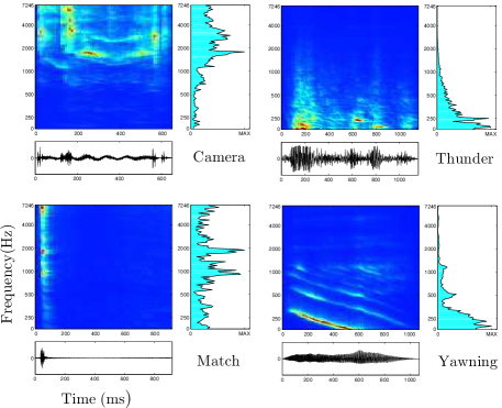
Figure 1: Spectrograms and fourier transforms of four sample sounds. The amplitude waveform of the sound is depicted below each spectrogram.

II-A Convolution model

The convolution model [1, 2, 3] is a linear mapping between the response of a population of neurons and a time-varying representation of the original stimulus, here spectrogram $s(t,f)$, sampled at times $t=1,...,T$ (see Fig. 1 for the spectrograms of four example sounds used in the study). The mapping is performed via a convolution of the neural responses evoked by the sound $r(t,x)$ with unknown spatio-temporal response functions $g(\tau,f,x)$

$$\hat{s}(t,f)=\sum_{x}\sum_{\tau}g(\tau,f,x)r(t-\tau,x)+\epsilon,$$ (1)

where $x$ indexes the MEG vertices (here sensors), $f$ represent the frequency channels, $\tau$ indicates the fixed duration (also referred to as the temporal lag above), and $\epsilon$ is an additive zero mean Gaussian random variable. In this model, the reconstruction for each frequency channel $\hat{s}_{f}$ is treated independently of the other channels. If we consider the reconstruction of one channel, it can be written as

$$\hat{s}_{f}(t)=\sum_{x}\sum_{\tau}g_{f}(\tau,x)r(t-\tau,x)+\epsilon.$$ (2)

To simplify the description of the inference algorithm used in this study, we transform the model in a linear algebraic form. First we define the response matrix $R\in\mathbb{R}^{NT\times\tau x}$, such that each row $r_{n}(t)$ contains the MEG response profile to sound $n$ across the entire set of sensors $x$ at time $t$ and the subsequent $\tau$ time bins:

$$R=$$

$$\begin{bmatrix}r_{1}(1,1)&r_{1}(1,2)&\cdots&r_{1}(1,x)&\cdots&r_{1}(1-\tau,x)\\ r_{1}(2,1)&r_{1}(2,2)&\cdots&r_{1}(2,x)&\cdots&r_{1}(2-\tau,x)\\ \vdots&\vdots&\ddots&\vdots\\ r_{1}(T,1)&r_{1}(T,2)&\cdots&r_{1}(T,x)&\cdots&r_{1}(T-\tau,x)\\ \vdots&\vdots&\vdots\\ r_{N}(T,1)&r_{N}(T,2)&\cdots&r_{N}(T,x)&\cdots&r_{N}(T-\tau,x)\\ \end{bmatrix}$$

$$G_{f}=\begin{bmatrix}g_{f}(1,1)&g_{f}(1,2)&\cdots&g_{f}(1,x)&\cdots&g_{f}(\tau,x)\end{bmatrix}^{\top}\\$$

and

$$S_{f}=\begin{bmatrix}s_{f}(1,1)&s_{f}(1,2)&\cdots&s_{f}(1,T)&\cdots&s_{f}(N,T)\end{bmatrix}^{\top}$$

Using the matrix notation, Eq 2 becomes: $S_{f}=RG_{f}+\epsilon$, which is similar to multiple linear regression with weights $G_{f}$. Given a pre-defined lag, the function $G_{f}$ is estimated by minimizing the mean-squared error between the actual and the predicted stimuli: $\mathop{\arg\min}_{G_{f}}\sum_{n,t}\{s_{f}(n,t)-\hat{s}_{f}(n,t)\}^{2}$. Solving this results in a maximum likelihood (ML) estimate:

$$\hat{G_{f}}=(R^{\top}R)^{-1}R^{\top}S_{f}.$$ (3)

The estimate requires an inversion of the inner product $R^{\top}R$ that has a dimension $d\times d$, where $d=\tau x$ is the dimension of the MEG response data. In neuroimaging, particularly in MEG, the value of $d$ is typically large. This is primarily due to the high spatial resolution of MEG where the data is sampled from hundreds to thousands vertices, $x$, depending on whether the data is represented at the sensor- or source-level. Further, the different sources can be highly correlated in MEG which makes the inversion ill-conditioned, i.e., the resulting inverse may not be possible to compute or it may be very sensitive to slight variation in the data.

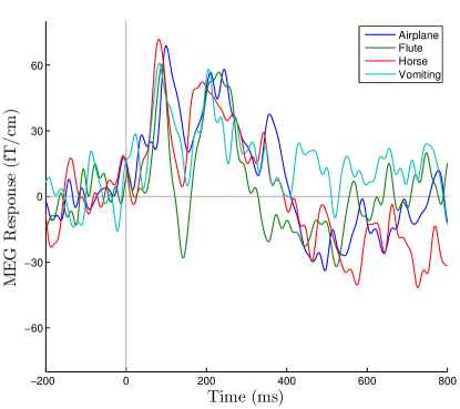
Figure 2: Event-related responses in one subject (averaged over 20 repetitions of the sound) at an MEG sensor located over the left hemisphere.

II-B Kernel convolution model

By applying similar developments for linear regression [6], we reformulate the classical convolution model in terms of its kernel or dual representation and add suitable regularization. In this representation, we use a sparse prior on the response function $G_{f}:G_{f}\sim N(0,\lambda_{f}^{-1}\mathrm{I})$, where $\lambda_{f}\geq 0$ is the regularization parameter and $\mathrm{I}$ is an identity matrix. The function can be determined by maximizing the log-posterior distribution of $G_{f}$ which is equivalent to minimizing the regularized sum-of-squares error function given by

$$\mathop{\arg\min}_{G_{f}}\sum_{n,t}\{s_{f}(n,t)-\hat{s}_{f}(n,t)\}^{2}+\lambda_{f}\sum_{x,\tau}g_{f}(\tau,x)^{2}.$$ (4)

Solving this yields a maximum a posteriori (MAP) estimate:

$$\hat{G_{f}}= (R^{\top}R+\lambda_{f}\mathrm{I})^{-1}R^{\top}S_{f}.$$ (5)

The addition of the regularization term stabilizes the estimation of the inverse. Following the derivation of kernel ridge regression [7], the MAP estimate can be obtained using the dual form of the sparse convolution model:

$$\hat{G_{f}}= R^{\top}(RR^{\top}+\lambda_{f}\mathrm{I})^{-1}S_{f}.$$ (6)

Unlike the original form (Eq. 5 or the non-sparse version: Eq. 3) that required the inversion of $R^{\top}R\in\mathbb{R}^{(\tau x)\times(\tau x)}$, the dual form requires inversion of the Gram matrix $K=RR^{\top}\in\mathbb{R}^{(NT)\times(NT)}$. This is very useful for neuroimaging studies where the number of conditions, $N$, is typically very low compared to the number of neural sources $x$ while $\tau$ and $T$ are of the same order. To estimate $\lambda_{f}$, we follow [8] and use an efficient computational technique [9], which avoids the inversion $(RR^{\top}+\lambda_{f}\mathrm{I})^{-1}$ for each value of $\lambda_{f}$ and uses a fast scoring measure to estimate leave-one-out error for different values of the regularization parameter.

The entire reconstruction of the sound spectrogram can be described as the collection of convolution functions for each frequency channel; $\hat{G}=[\hat{G_{1}}\hat{G_{2}}\cdots\hat{G_{F}}]$. Then, given an MEG response to a test sound, we take the lagged representation of the response, $r_{\text{new}}\in\mathbb{R}^{T\times(\tau x)}$, and obtain a prediction of its spectrogram $\hat{S}_{\text{new}}\in\mathbb{R}^{T\times F}$ as follows:

$$\hat{S}_{\text{new}}=r_{\text{new}}\hat{G}=r_{\text{new}}R^{\top}(RR^{\top}+\lambda_{f}\mathrm{I})^{-1}S.$$ (7)

The dual formulation can be obtained by noticing that the prediction in Eq. 7 operates on the feature space and only involves inner products. These inner products can be replaced with a kernel function $k(r_{n},r_{m})=\mathbf{\phi}(r_{n})^{\top}\mathbf{\phi}(r_{m})=\sum_{i}\phi_{i}(r_{n})\phi_{i}(r_{m})$, where $\phi_{i}(r)$ are the basis functions. If we substitute the kernel functions for the inner-products we obtain the following prediction of the spectrogram: $\hat{S}_{\text{new}}=\text{k}(r_{\text{new}})(K+\lambda_{f}\mathrm{I})^{-1}S$, where we have defined the matrix $\text{k}(r_{\text{new}})$ with column-wise concatenation of submatrices $k(r_{\text{new}},r_{n})$. Similarly, the submatrices of $K$ are defined using the kernel function $k(r_{n},r_{m})$. Thus, the dual formulation implicitly allows to use feature spaces of very high, even infinite, dimensions.

II-C Model evaluation

We performed a leave-two-out cross-validation where, in each fold, we used all but two randomly picked sounds as training data. To label the held-out sounds without using any training examples for those sounds, we followed a two-stage prediction procedure, similar to [10]. In the first stage, we applied the learned functions to predict the spectrograms for the test sound pair and concatenated the temporal dimension to form vectors for both predicted and original spectrograms. In the second stage, we quantified the predictive accuracy by computing the correlation between the reconstructed and the original spectrogram of the two test sounds. If the two predictions are represented as $p_{1}$ and $p_{2}$ and the original spectrograms are $s_{1}$ and $s_{2}$, then the labelling assigned by the model was considered correct if:

$$\mbox{corr}(s_{1},p_{1})+\mbox{corr}(s_{2},p_{2})>\mbox{corr}(s_{1},p_{2})+\mbox{corr}(s_{2},p_{1})$$ (8)

This process is repeated for all possible combinations of leave-two-out sounds. Under this evaluation, the expected performance of a random model is $50\%$. Since the sounds are of different durations, to evaluate Eq. 8, we truncated the predicted and original spectrogram to the length of the shorter sound in each test sound pair.

To evaluate how well the spectrogram features were predicted, we use the following score:

$$\mbox{score}_{f,t}=1-\frac{\sum(s_{f,t}-\hat{s}_{f,t})^{2}}{\sum(s_{f,t}-\bar{s}_{f,t})^{2}},$$ (9)

where $s_{f,t}$ is the original value of the spectrogram frequency $f$ at time $t$, $\hat{s}_{f,t}$ is the predicted value by the model, and $\bar{s}_{f,t}$ is the mean value across all pairs in the cross-validation combinations. The summations in Eq. 9 are computed over all pairs of cross-validation samples. The feature score thus measures percent of variation explained in each feature.

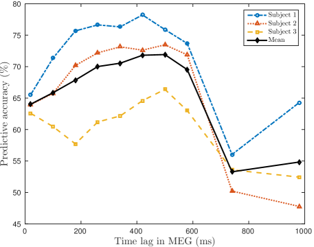
Figure 3: Performance of kernel convolution model as a function of time-lag. Each point is an average over 946 cross-validation tests. Chance accuracy is 50%. Solid line is average accuracy across the three subjects.

III Experiments

III-A MEG recordings

The data consisted of event-related MEG responses from three subjects listening to common environmental sounds ($44$ items). The sounds included sets of $6-8$ items from five pre-selected categories (vehicles, music, human, animal and tool) and $8$ uncategorized sounds. Each sound was presented $20$ times.

Magnetic fields associated with neural current flow were recorded with a $306$-channel whole-head neuromagnetometer (Elekta Oy, Helsinki) in the Aalto NeuroImaging MEG Core. The MEG signals were band-pass filtered between $0.03$ and $330$ Hz and sampled at $1000$ Hz. During the recordings subjects listened to a pseudo-randomly shuffled sequence of sounds and were asked to respond by finger lift when two consecutive sounds referred to the same item. Response trials were excluded from analysis. The event-related responses to the $20$ repetitions of each stimulus were averaged from $300$ ms before to $2000$ ms after the stimulus onset, rejecting trials contaminated by eye movements. On average $19.2\pm 1.1$ (mean $\pm$ standard deviation) artifact-free epochs (repetitions) per subject were gathered for each item. The averaged MEG responses were baseline-corrected to the $200$ ms interval immediately preceding the stimulus onset and down-sampled to $10$ ms intervals. Data analysis was restricted to $56$ planar gradiometers above the auditory cortex. Example responses are depicted in Fig. 2.

III-B Stimulus spectrogram representation

The auditory spectrogram representation was binned at $10$ ms and calculated based on the auditory filter bank with $128$ overlapping bandpass filter channels mimicking the auditory periphery [11]. Filters had logarithmically spaced central frequencies ranging from $180$ to $7246$ Hz (Fig. 1).

III-C Prediction of sound spectrograms from MEG responses

Prior to the analysis, both spectrogram and MEG data were standardized to zero mean and unit variance. We used causal response functions ($\tau\leq 0$; [4]), which means that the model decoded spectrograms of sounds at time $t$ using neural responses at time $t,t+1,t+2,...,t-\tau$ ms. To evaluate the sensitivity of MEG neural responses to the frequencies in the stimulus spectrogram, we evaluated the mean predictive accuracy across all possible leave-two-out combinations of $44$ sounds ($C_{2}^{44}=946$ combinations) for different time-lags $-\tau$ = $20$, $100$, $180$, $260$, $340$, $420$, $500$, $580$, $740$ and $980$ ms. Results, shown in Fig. 3, indicate that it was possible to discriminate between two previously unencountered test sounds with $\sim 70\%$ accuracy (Mean value $70.0$ to $71.9$ at time-lag $250$ to $500$ ms) even when neither sound was used in the training data. Next, to evaluate which spectrogram features were best predicted, we considered the time-lag of $500$ ms that gave the optimal predictions and computed the mean score (Eq 9) across the three subjects for each spectrogram feature. The top $15$ scoring features represent high stimulus frequencies (above $3.8$ kHz) with scores ranging from $0.12$ to $0.21$. Further, we computed item-wise mean predictive accuracy over the cross-validation folds. The five best predicted sounds were camera $(95.3\%)$, helicopter $(88.4\%)$, lighting a match $(84.5\%)$, motorsaw $(83.7\%)$, and door $(82.9\%)$, while five least accurately predicted sounds were trumpet $(59.7\%)$, laughter $(58.9\%)$, yawning $(56.6\%)$, zipper $(55.0\%)$, and thunder $(54.3\%)$. The best predicted sounds typically contained higher frequencies compared to the less accurately predicted sounds (see Fig. 1).

IV Discussion and Conclusion

Our results demonstrate that the kernel convolution model provides an efficient method for predicting spectrograms of new sounds. Predictions are made by decoding neural information in high-dimensional MEG responses to common environmental sounds. Therefore, the extracted neural information can be regarded as being based on neural mechanisms that generalize across a variety of sounds. We evaluated different time-lags in the MEG response data to predict spectrograms of unencountered sounds, and observed that the responses are most sensitive for a duration of around $250-500$ ms from the input stimulus. The auditory evoked responses used in the analysis are most prominent at $50-500$ ms after the stimulus onset despite the stimulus duration (see Fig. 2). Thus, at the longest time-lags ($>500$ ms) the MEG data is noisier compared to shorter lags, as the decaying MEG responses start to show large inter-response variability. Neurophysiological interpretation and evaluation of significance of the results are natural extensions of the study. The decoding problem studied here is an example of an underdetermined systems for which regularization and Bayesian inference have provided reasonable answers.

Classical linear regression has been used earlier to decode neural responses, but most studies have either been limited to non-time-varying stimulus representations [8] or neuroimaging recordings [10] [12]. The proposed method will be useful for analyzing brain’s ability to understand sounds in an acoustic environment, particularly when neural responses are recorded at high spatio-temporal resolution.

References

- [1] W. Bialek, F. Rieke, R. van Steveninck, and D. Warland, “Reading a neural code,” Science, vol. 252, pp. 1854–1857, 1991.
- [2] N. Mesgarani, S. David, J. Fritz, and S. Shamma, “Influence of context and behavior on stimulus reconstruction from neural activity in primary auditory cortex,” Journal of Neurophysiology, vol. 102, pp. 3329–3339, 2009.
- [3] B. Pasley et al., “Reconstructing speech from human auditory cortex,” PLoS Bio., vol. 10, no. 1, p. e1001251, 2012.
- [4] N. Mesgarani and E. Chang, “Selective cortical representation of attended speaker in multi-talker speech perception,” Nature, vol. 485, pp. 233–236, 2012.
- [5] A. Calabrese, J. Schumacher, D. Schneider, L. Paninski, and S. Woolley, “A generalized linear model for estimating spectrotemporal receptive fields from responses to natural sounds,” PLoS One, vol. 6, p. e16104, 2011.
- [6] T. Hastie, R. Tibshirani, and J. Friedman, The elements of statistical learning. Springer, 2001.
- [7] C. Bishop, Pattern recognition and machine learning. Springer, 2006.
- [8] G. Sudre et al., “Tracking neural coding of perceptual and semantic features of concrete nouns,” NeuroImage, vol. 62, pp. 451–463, 2012.
- [9] I. Guyon, “Kernel ridge regression tutorial,” Notes on Kernel Ridge Regression. ClopiNet, Tech. Rep., 2005.
- [10] T. Mitchell et al., “Predicting human brain activity associated with the meanings of nouns,” Science, vol. 320, pp. 1191–1195, 2008.
- [11] T. Chi, P. Ru, and S. Shamma, “Multiresolution spectrotemporal analysis of complex sounds,” The Journal of the Acoustical Society of America, vol. 118, pp. 887–906, 2005.
- [12] R. Santoro et al., “Encoding of natural sounds at multiple spectral and temporal resolutions in the human auditory cortex,” PLoS Comp. Bio., vol. 10, p. e1003412, 2014.