Creating an Artificial World with a New Kind of Cellular Automaton

Abstract

This paper describes a new concept of cellular automaton (CA). XCA consists of a set of arcs (edges) that correspond to cells in CA. At a particular time, the arcs are connected to a directed graph. With each time step, the arcs exchange their neighbors (adjacent arcs) according to rules that depend on the statuses of the adjacent arcs.

An XCA can be used to simulate an artificial world beginning with a Big Bang. In contrast to an CA, an XCA does not require a grid. However, it can create one, just as the real universe after the Big Bang generated its own space, which had not excisted previously. Examples using different rules reveal the manifold nature of the XCA concept. Similar to John Conway’s well-known The Game of Life simulates birth, survival, and death, this game can simulate a system that begins from a singularity, and evolves into a complex space.

Keywords: Big Bang, cellular automaton, The Game of Life, mathematical games, complex systems, graph theory, dynamical graph, graph drawing, space time, digital physics, cosmology

Contents

1. 1 Introduction
2. 2 CA
3. 3 XCA
   1. 3.1 Cellular Rules
   2. 3.2 Transition Rules
   3. 3.3 Decision and Constraint Rules
   4. 3.4 Connectivity
4. 4 Turing Machine
5. 5 XCA Rule Examples
   1. 5.1 Rule Example 1
   2. 5.2 Rule Example 2
      1. 5.2.1 Configuration 1:
      2. 5.2.2 Configuration 2:
      3. 5.2.3 Configuration 3:
   3. 5.3 Rule Example 3
   4. 5.4 Rule Example 4
   5. 5.5 Rule Example 5
   6. 5.6 Rule Example 6
      1. 5.6.1 Configuration of AND/OR Gate:
      2. 5.6.2 Configuration of NOT Gate
   7. 5.7 Rule Example 7 - Copy Machine/Oscillator
      1. 5.7.1 Copy Machine
      2. 5.7.2 Oscillator
   8. 5.8 Rule Example 8
6. 6 Signals, Information Arcs, ad Information Pulses
7. 7 Visualization
8. 8 Artificial World
   1. 8.1 Space/Grid
   2. 8.2 Attraction/Repulsion
   3. 8.3 Virtual Dimension
   4. 8.4 Time Aspects
      1. 8.4.1 Step-based Time
      2. 8.4.2 Event Time
      3. 8.4.3 Space Time
   5. 8.5 Elementary Particles
9. 9 Conclusion
10. 10 Acknowledgement
11. A Appendix
    1. A.1 Cellular Automaton
    2. A.2 Adjacency Matrix, Incidence Matrix, Incidence List
    3. A.3 PSEUDO CODES OF THE BIG BANG GAME
       1. A.3.1 BIG BANG GAME
       2. A.3.2 Transition
       3. A.3.3 CONVERT INCIDENCE LIST TO ADJACENCY MATRIX
       4. A.3.4 CONVERT ADJACENCY MATRIX TO INCIDENCE MATRIX
       5. A.3.5 CONVERT INCIDENTS MATRIX TO INCIDENCE LIST

Weil im Schoenbuch

1 Introduction

This paper describes a new concept of cellular automaton (CA), the extended CA (XCA), which leads to two paradigm shifts: 1) a more generalized definition of cell, and 2) different roles for the nodes and arcs of a network.

Definition-of-Cell:

In general, a cell is understood as the face of a two-dimensional grid, or more generally, as the n-dimensional solid of an n-dimensional grid. An XCA requires a more generalized definition of a cell as follows: 1) a cell is surrounded by borders 2) any two neighboring cells have a common border. - With this definition. not only the fields of a grid, but also the nodes and arcs (edges) of a graph can be considered to be cells.

Nodes-and-Arcs:

Normally, the nodes of a graph represent objects, and the arcs are seen as connections between objects. With our XCA view, in contrast to the standard view, the arcs are seen as objects, which are connected at nodes. With this concept, the number of arcs remains constant, while the number of nodes may change with each step of evolution.

In addition to the classical concept of CA, there are other concepts of CA in which nodes are considered cells. Two neighboring nodes have an arc as a common border. In contrast to this concept for the arc-based XCA, two neighboring arcs have a node as a common border.

For each time step, the value of each cell changes according to the values of the neighboring cells and according to some transition rules. This is true for both concepts. However, in contrast to a CA, an XCA can exchange the neighbors (adjacent arcs) according to rules that depend on the statuses of adjacent arcs.

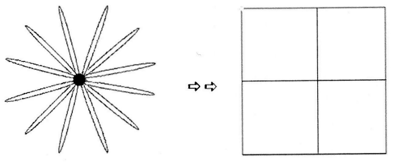
The new model might help to explain physical phenomena. At the beginning of the universe, all arcs are connected with both ends to a single node. With the next discrete time steps, the graph alters its structure, while the arcs maintain their identities (Figure 1). According to this hypothesis, all phenomena are represented by different configurations and evolutions of arcs. However, not only matter, particles, and interactions, but also space itself, are represented by arcs.

Figure 1: Big Bang Model

2 CA

In 1970 John H. Conway published “The Game of Life” [1], which soon gained much popularity. This "game" is the best-known example of a CA[2]. “The Game of Life (or simply Life) is not a game in the conventional sense. There are no players, and no winning or losing. Once the ‘pieces’ are placed in the starting position, the rules determine everything that happens later” [3]. The ‘game’ is a zero-player game, meaning that its evolution is determined by its initial state, requiring no further input from humans. One interacts with The Game of Life by creating an initial configuration and observing how it evolves.” [4]

Life is an example of self-organization [5].

A CA consists of an n-dimensional grid, whose cells are assigned specific values at particular times. For each time step, the value of each cell changes according to the values of the neighboring cells (usually including the cell itself) and according to some transition rules. Different examples of a CA show how chaos can evolve into a structured organization.

For some examples, visit http://www.collidoscope.com/modernca/ [6]. You can find an introduction to the general concept of CA in Appendix A.1.

Inspired by the idea of CA, I developed an XCA with which an artificial world can be simulated beginning with a Big Bang. In contrast to a CA, an XCA does not require a grid. However, it can create one, just as the real universe after the Big Bang generated its own space, which had not existed previously.

3 XCA

The arcs of an XCA correspond to the cells in CA. At a particular time, the arcs are connected to a directed graph. Arcs that are connected to a node are neighbors. Just as values are assigned to cells of a CA, particular values can be assigned to the endpoints of an arc. With each time step, the arcs exchange their neighbors (adjacent arcs) according to rules that depend on the statuses of adjacent arcs.

Let us denote the start point (head) and end point (tail) of arc $A$ by $A_{1}$ and $A_{0}$, respectively. The values $V(A_{0})$ and $V(A_{1})$ can be assigned to the start and end points, respectively, and $V(A)$ to the arc itself. At a particular time, two arcs $A$ and $B$ meet at a node with their start and end points $A_{1}$ and $B_{0}$, respectively. The state of the node is then denoted as $\left\{A_{1},\,B_{0}\right\}$, or alternatively, as $A_{1}B_{0}$.

An XCA game is described using four types of rules:

• Cellular rules

• Transition rules

• Decision and constraint rules

• Connectivity

3.1 Cellular Rules

Cellular rules apply to the values $V(x)$ and correspond to the transition rules applied to the cell values of a conventional CA. Consider the dual graph of a rectangular grid. XCA and CA are then equivalent in the following conditions:

• The grid does not change its topology in discrete time steps.

• The nodes in the dual graph correspond to cells, and arcs designate neighbors of the CA.

• If the arcs $a$, $b$, $c$, and $d$ meet at node {$a_{1},b_{0},c_{0},d_{1}\}$, then $V(a_{1})=V(b_{0})=V(c_{0})=V(d_{1})$.

3.2 Transition Rules

Two arcs can be linked to a node in four possible manners: $A_{1}B_{0}$, $A_{0}B_{1}$, $A_{1}B_{1}$, and $A_{0}B_{0}$.

For $A_{1}B_{1}$, for example, there are four possible transition rules regarding how the links can change with the next time step:

• • $A_{1}B_{1}->A_{1}B_{1}$(no change) $\Rightarrow$ -----$A$--->.<---$B$-----

    $A_{1}B_{1}->A_{1}B_{0}$ $\Rightarrow$ -----$A$--->.-----$B$---->

    $A_{1}B_{1}->A_{0}B_{1}$ $\Rightarrow$ <----$A$----.<----$B$-----

    $A_{1}B_{1}->A_{0}B_{0}$ $\Rightarrow$ <----$A$----.-----$B$---->

The two arcs can also be linked together at both sides (multiple arcs) at the same time, for instance, at $A_{1}B_{1}$ and $A_{0}B_{0}$ to produce a state denoted as $A_{1}B_{1}/A_{0}B_{0}$. Figures 2 and 3 show the states $A_{1}B_{1}/A_{0}B_{0}$ and $A_{1}B_{0}/A_{0}B_{1}$, respectively.

Figure 2:

Figure 3:

An arc can also be linked to itself with node $\left\{A_{1}A_{0}\right\}$ by building a circle (loop). The end points $A_{1}$ and $A_{0}$ can connect and disconnect from step to step. If the loop of $A$ is linked to the arc $B$, then the following transition is possible:
$\left\{A_{i},\,A_{k},\,B_{i}\right\}\Rightarrow\left\{A_{i},\,B_{i}\right\}/\left\{A_{k}\right\}$ (the loop opens)

In general, the following transition rules are possible for state $A_{i}B_{k}$, where $i$ and $k$ are either zero or one, and $i$ is not $k$:

$A_{i}B_{k\,}$$\Rightarrow$ $A_{i}B_{k}$ (no change)

$A_{i}B_{k\,}$$\Rightarrow$ $A_{i}B_{i}$

$A_{i}B_{k}$ $\Rightarrow$ $A_{k}B_{k}$

$A_{i}B_{i}$ $\Rightarrow$ $A_{i}B_{i}$ (no change)

$A_{i}B_{i}$ $\Rightarrow$ $A_{i}B_{k}$

$A_{i}B_{i}$ $\Rightarrow$ $A_{k}B_{i}$

3.3 Decision and Constraint Rules

Consider the transition rule $A_{1}B_{1}$$\Rightarrow$$A_{1}B_{0}$ being applied to the arcs $a$, $b$, and $c$, meeting at point ${a_{1},b_{1},c_{1}}$. Arc $a$ can interact with either $b$ or $c$, indvidually or with both $b$ and $c$ at the same time. If $a$ interacts with $b$, then there are two possible manners in which the arcs can interact with the next time step:

$a_{1}b_{1}$ $\Rightarrow$ $a_{1}b_{0}$

$b_{1}a1$ $\Rightarrow$ $b_{1}a_{0}$

This example above shows why decision rules are necessary.

Examples of Decision Rules:

1. The arcs interact by chance with preferences.

2. The transition is controlled by the statuses of neighboring arcs.

3. The status of time step t must not be equal to that of time step t +2. Otherwise, the arcs interact by chance.

4. Each arc is identified by a number. At even time step t, the lower numbered arc has priority. At odd time step t +1, the higher numbered arc has priority.

5. The transition is controlled by cellular rules.

6. Consider the arcs $a$, $b$, $c$, and $d$ are connected at the nodes $d_{1}c_{0}$, $c_{1}b_{0}$, $b_{1}a_{0}$. By the transition rules $d_{1}c_{0}$ $\Rightarrow$ $d_{1}c_{1}$, $c_{1}b_{0}$ $\Rightarrow$ $c_{1}b_{1}$, and $b_{1}a_{0}$ $\Rightarrow$ $b_{1}a_{1}$ the arcs will meet at node ${d_{1},c_{1},b_{1},a_{1}}$. Now the arc $c$ becomes a neighbor of $a$. The fact that $d$ is a new neighbor of $a$ can be understood as $d$ being ranked lower than $b$ and $c$. This ranking can also be a criterion for a decision rule.

Examples of Constraints:

1. Transitions cannot allow multiple arcs (two arcs being connected at both ends, see Figures 2 and 3 above).

2. Transitions cannot allow circles (self loops).

3. Transitions cannot allow reversing, meaning that the status of two arcs at time step t +1 cannot be the same as at time step t -1.

4. Transitions cannot allow multiple interactions, meaning that an arc cannot interact with more than one other arc at the same time step.

5. Any two linked arcs must change their status at every time.

3.4 Connectivity

An XCA graph must not be disconnected at any time step. For a connected graph, this condition is always true as long as no transition rule causes a disconnection. If a node $A_{i}B_{k}$ exists, then no transition is allowed that disconnects A and B, with one exception:

Let us assume that the three arcs $A$, $B$, and $C$ are connected together with one of their end points. The arc $A$ can then move to the other end of $B$, thus disconnecting $A$ from $C$. In this case, the transition $AC\Rightarrow 0$ is allowed.

4 Turing Machine

A Turing machine models the operation of a computer in a particularly simple and mathematically analyzable manner.

The machine consists of a tape with an endless sequence of symbols. At each time step, a tape head reads a single symbol on the tape. Depending on this symbol, the status of the tape head, and a set of instructions, the tape head overwrites the symbol with a new one. Then, it moves to the next symbol either to the left or to the right.

An XCA configuration can emulate a Turing machine. A chain of arcs whose start points are all in the same direction, represents the tape. The arcs represent symbols of the tape and do not interact with each other. A different arc behaves in a manner similar to that of the tape head that meets the start point of an arc of the chain. Depending on the value of the symbol arc, the status of the tape head arc, and a set of instructions, the value of the symbol arc is replaced by a new one. Then the tape head arc moves either to the left or to the right of the symbol arc.

In general, any three arcs of a node in an XCA system can be seen as a type of Turing machine. Two of the arcs correspond to neighboring symbols of the machine. The third arc corresponds to the tape head. This type of machine is valid for only a limited time. After this time, the roles of the arcs can be interchanged. One of the former symbol arcs becomes the tape head arc and the previous tape head arc becomes a symbol arc.

Finally, each arc of an XCA can resemble a computer, processing its neighbors.

5 XCA Rule Examples

I like to believe, that XCAs will make it possible to simulate the physical world, provided that appropriate rules are found. This is not yet the case, but the following examples will show how multifold this system is.

5.1 Rule Example 1

The arcs interact by chance.

There are no constraints.

The graph must not be disconnected at any time step.

Start Configuration:

At the beginning, all arcs are connected with both ends to a single node.

Figure 4: Big Bang Model

Because any arc with both ends connected to a single node is adjacent to any other arc, the arbitrary transitions can result in any possible configuration. In Figure 4, the initial graph with 12 arcs evolves into a rectangular grid with 12 arcs by chance. With the same probability, any other configuration is possible, provided that the number of arcs remains constant, and the graph is not disconnected.

5.2 Rule Example 2

Consider the following transition rules:

$A_{1}B_{1}$ $\Rightarrow$ $A_{0}B_{1}$;

$A_{0}B_{1}$ $\Rightarrow$ $A_{0}B_{0}$;

$A_{0}B_{0}$ $\Rightarrow$ $A_{1}B_{0}$;

$A_{1}B_{0}$ $\Rightarrow$ $A_{1}B_{1}$;

As constraints, the transitions do not allow the following:

1. multiple arcs (two arcs being connected at both ends, see Figures2 and 3above)

2. circles

3. reversing (the status of two arcs at time step t +1 being the same as at time step t -1)

4. multiple interactions (an arc interacting with more than one other arc at the same time step)

We can apply these rules to different configurations as follows.

5.2.1 Configuration 1:

The two arcs $a$ and $b$ meet at point $a_{1}b_{0}$ at the first time step. Figure 5 shows steps 0 through 3 (step 4 is equal to step 0).

Figure 5:

The following figures show how the graphs of consecutive time steps evolve through intermediate steps being inserted. In Figure 6, for instance, two intermediate steps are inserted. The two arcs $a$ and $b$ meet at point $a_{1}b_{0}$ at the first time step. Figure 6 shows how the start point of arc $a$ (vertical) moves from the end point $b_{0}$ to the start point $b_{1}$, passing the two intermediate points between $b_{0}$ and $b_{1}$.

Figure 6:

5.2.2 Configuration 2:

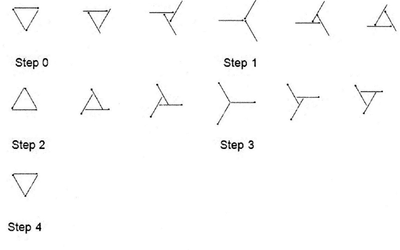
At the first time-step, the three arcs a, b, and c form a triangle with the nodes a1b0, b1c0, and c1a0. In Figure 7 four steps are displayed. Intermediate steps show the movements from step to step.

Figure 7:

5.2.3 Configuration 3:

The initial graph consists of the nodes $\{b_{0},a_{1}\},\{a_{0},c_{0},d_{1}\},\{d_{0},e_{1}\},\{f_{1},e_{0}\},\{b_{1},c_{1},f_{0}\}$ as shown in Figure 8,

Figure 8:

The pairs of arcs change their relations according to the following transition rules:

$a_{0}c_{0}$$\Rightarrow$ $c_{1}a_{0}$

$c_{0}d_{1}$$\Rightarrow$$d_{0}c_{0}$

$d_{1}a_{0}$$\Rightarrow$$a_{1}d_{1}$

$b_{1}f_{0}$$\Rightarrow$$f_{1}b_{1}$

$f_{0}c_{1}$$\Rightarrow$$c_{0}f_{0}$

$c_{1}b_{1}$$\Rightarrow$$b_{0}c_{1}$

$b_{0}a_{1}$$\Rightarrow$$a_{0}b_{0}$

$e_{0}f_{1}$$\Rightarrow$$f_{0}e_{0}$

$d_{0}e_{1}$$\Rightarrow$$e_{0}d_{0}$

$f_{1}e_{0}$$\Rightarrow$$e_{0}f_{0}$

From the new pairs, the following nodes will result:

$\{b_{0},a_{0},c_{1}\},\{b_{1},f_{1}\},\{a_{1},d_{1}\},\{f_{0}$, c₀, d₀, e${}_{0}\}$

The new graph, shown in Figure 9, is the dual graph of the initial graph.

Figure 9:

In Figure 10, four steps are displayed. Intermediate steps show the movements from step to step.

With this rule, planar graphs remain planar after all transitions. Nonplanar graphs become planar.

Figure 10:

5.3 Rule Example 3

The graph consists of colored arcs with the colors $a$, $b$, and $c$.

The following rules apply for links between arcs of the same color:

$B_{a1}A_{a1}\Rightarrow A_{a0}B_{a1}\Rightarrow B_{a0}A_{a2}\Rightarrow A_{a1}B_{a0}\Rightarrow B_{a1}A_{a1}$

$A_{a1}B_{a1}\Rightarrow B_{a0}A_{a1}\Rightarrow A_{a0}B_{a0}\Rightarrow B_{a0}A_{a1}\Rightarrow A_{a1}B_{a1}$

$B_{b1}A_{b1}\Rightarrow A_{b0}B_{b1}\Rightarrow B_{b0}A_{b0}\Rightarrow A_{b1}B_{b0}\Rightarrow B_{b1}A_{b1}$

$A_{b1}B_{b1}\Rightarrow B_{b0}A_{b1}\Rightarrow A_{b0}B_{b0}\Rightarrow B_{b0}Ab1\Rightarrow A_{b1}B_{b1}$

Between arcs of color $c$, there is no interaction.

Between arcs of the colors $c$ and $a$, the following transition rule applies:

$A_{a1}B_{c1}\Rightarrow A_{a1}B_{c0}\Rightarrow A_{a1}B_{c1}$

Between arcs of the colors $c$ and $b$, the following transition rule applies:

$A_{b1}B_{c1}\Rightarrow A_{b0}B_{c1}\Rightarrow A_{b1}B_{c1}$

Arcs of the same color other than c can interact with higher priority; otherwise, the arcs interact with their neighbors by chance.

Configuration:

According to color, the graph can consist of four arcs, which meet at a central node.

$a_{a1},b_{a1},c_{a1},d_{a1}$

$e_{b1},f_{b1},g_{b1},h_{b1}$

$i_{c1},j_{c1},k_{c1},l_{c1}$

Figure 11:

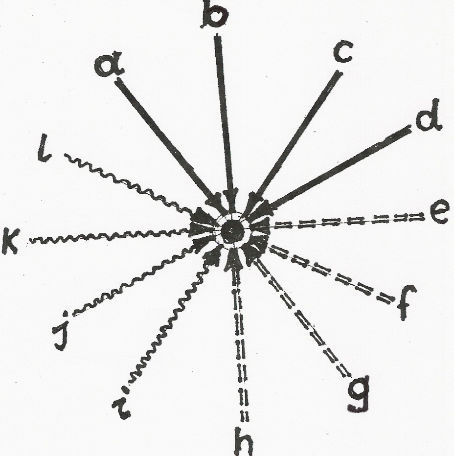
According to the transition rules, for example, the following configurations can evolve:

$a_{a1}b_{a1}\Rightarrow a_{a1}b_{a0}$

$b_{a1}c_{a1}\Rightarrow b_{a1}c_{a0}$

$c_{a1}d_{a1}\Rightarrow c_{a1}d_{a0}$

$d_{a1}a_{a1}\Rightarrow d_{a1}a_{a0}$

$a_{a1}i_{c1}\Rightarrow a_{a1}i_{c0}$

$b_{a1}j_{c1}\Rightarrow b_{a1}j_{c0}$

$c_{a1}k_{c1}\Rightarrow c_{a1}k_{c0}$

$d_{a1}l_{c1}\Rightarrow d_{a1}l_{c0}$

$e_{b1}f_{b1}\Rightarrow e_{b1}f_{b0}$

$f_{b1}g_{b1}\Rightarrow f_{b1}g_{b0}$

$g_{b1}h_{b1}\Rightarrow g_{b1}h_{b0}$

$h_{b1}e_{b1}\Rightarrow h_{b1}e_{b0}$

$f_{b1}l_{c1}\Rightarrow f_{b0}l_{c1}$

$g_{b1}k_{c1}\Rightarrow g_{b0}k_{c1}$

$h_{b1}j_{c1}\Rightarrow h_{b0}j_{c1}$

$e_{b1}i_{c1}\Rightarrow e_{b0}i_{c1}$

The resulting nodes are as follows:

$$\{a_{1},b_{0},i\},\{b_{1},c_{0},j_{0}\},\{c_{1},d_{0},k_{0}\},\{d_{1},a_{0},l_{0}\},$$

$$\{e_{1},f_{0},l_{1}\},\{f_{1},g_{0},k_{1}\},\{g_{1},h_{0},j_{1}\},\{h_{1},e_{0},i_{1}\}$$

Figure 12:

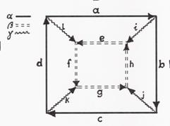
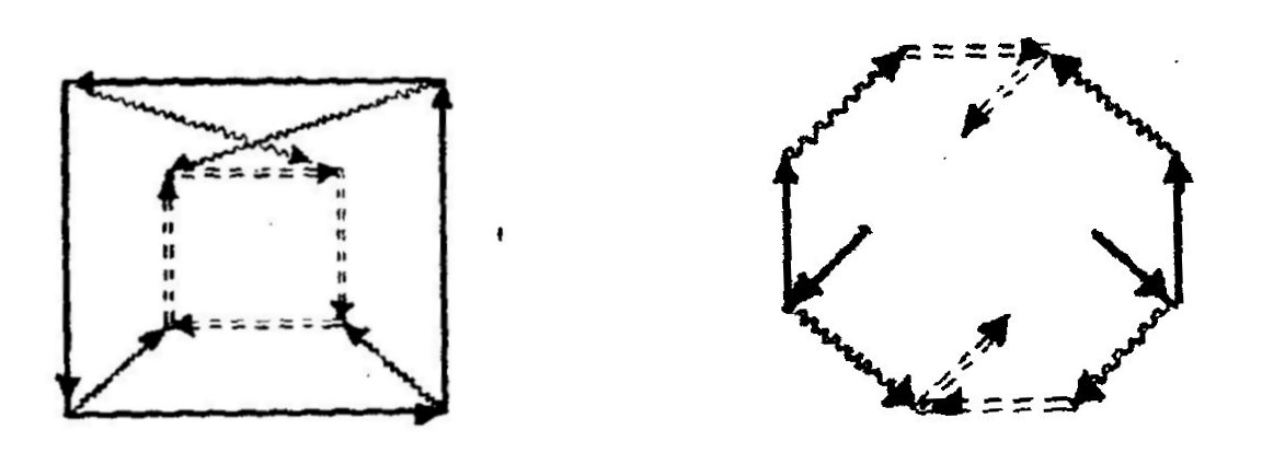
In Figure 13, step 0 is topologically equivalent to that in Figure 11 and step 1 is equivalent to that in Figure 12. Figure 13 shows the two steps. Intermediate steps show the movements from step to step.

Figure 13:

If the arcs interact by chance with their neighbors, independent of color, results such as those shown in Figure 14 are possible:

Figure 14:

5.4 Rule Example 4

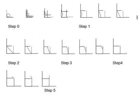
With this example, it can be shown, that a square grid can be created starting with a set of arcs. The set consists of paired arcs $P$ and normal arcs $N$. A pair $P_{x}$ consists of two arcs, $P_{xa}$ and $P_{xb}$, which are connected at a midpoint $P_{x0}$ (the connection of $P_{xa0}$ and $P_{xb0}$) and the end points $P_{xa1}$ and $P_{xb1}$. There is no interaction between the two arcs. If the midpoints of two pairs meet at the same point, one midpoint $P_{x0}$ moves to one of the end points of the other pair. Which pair moves to which end point of the other pair, is arbitrary. A normal arc interacts with the arcs of a pair as follows:

• A normal arc $N_{a}$ interacts alternately with the arcs of a pair $P_{x}$. When the one end of the arc $N_{a}$ interacts, the other end is inactive, and vice versa.

• If the active end point of $N_{a}$ coincides with the midpoint of the pair $P_{x}$, then this end point will move to one of the end points of the pair $P_{x}$.

• If the active end point of $N_{a}$ coincides with the end point of the pair $P_{x}$ and the midpoint of another pair $P_{y}$, then this active point will move to one of the end points of the new pair $P_{y}$.

• If the active point coincides with an end point of a pair, and this point is not connected with another pair, then the end point of the pair will move to the other point of the normal arc $N_{a}$.

The transition rules between two normal arcs might not be relevant for this example.

Configuration:

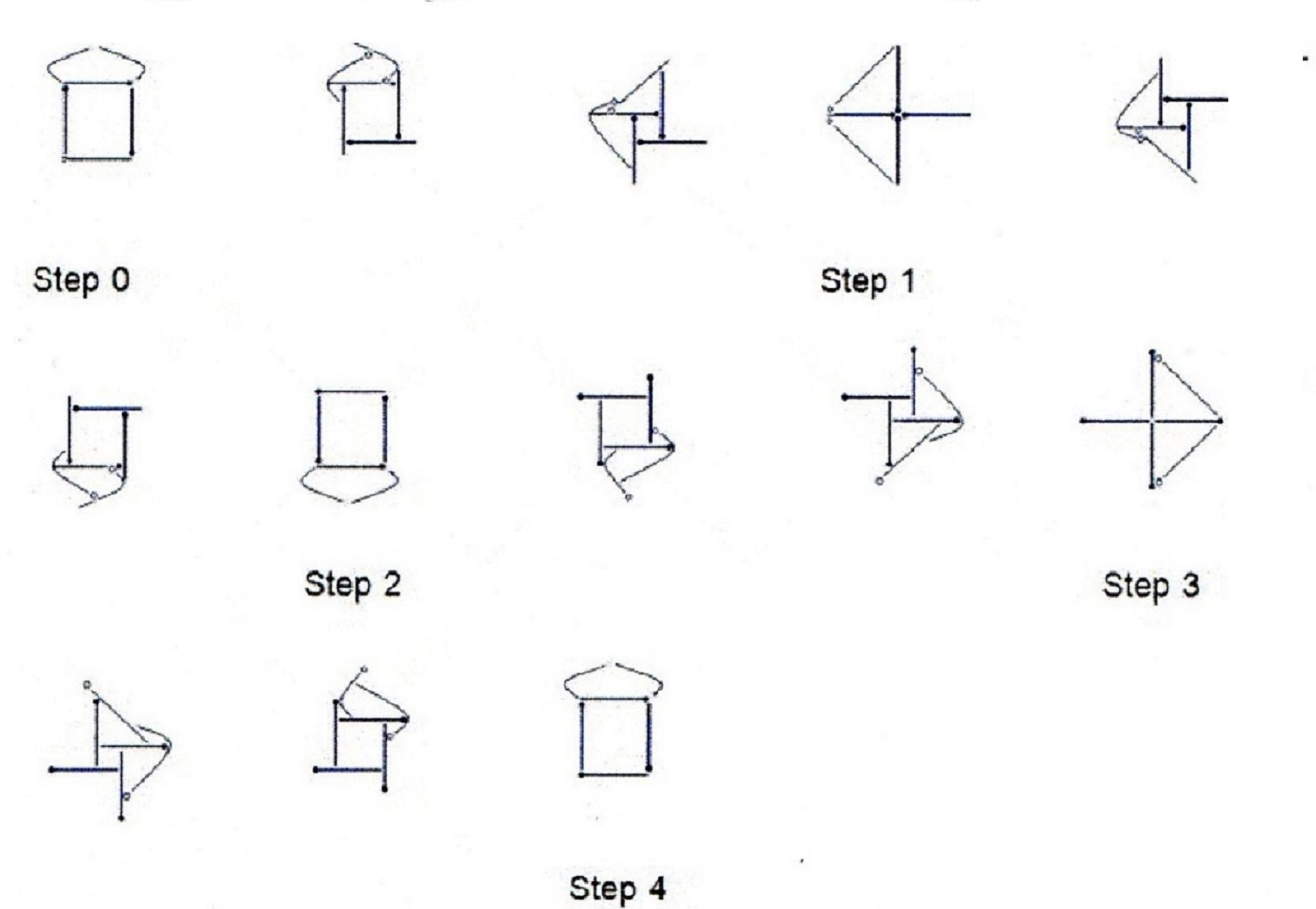
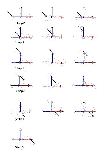
A set of paired arcs and normal arcs meet at a central node. The evolution to a square grid cell is shown in the series of Fgure 15, steps zero through five.

Figure 15:

5.5 Rule Example 5

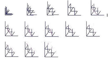
With this example, it will be proved that the creation of a cubic grid starting with a set of arcs is possible. This example is analogues to Example 4. The set consists of triple arcs $T$ and normal arcs $N$.

A triple $T_{x}$ consists of three arcs $T_{xa}$, $T_{xb}$, and $T_{xc}$, which are connected at a midpoint $T_{x0}$, and the end points $T_{xa1}$, $T_{xb1}$, and $T_{xc1}$. There is no interaction between the three arcs. If the midpoints of two triplets meet at the same point, then one midpoint $T_{x0}$ moves to one of the end points of the other triplet. Which triplet moves to which end point of the other triplet is arbitrary. The rules regarding how a normal arc interacts with an arc of a triplet are the same as those in Example 4.

Configuration:

The elements of a set of triple and normal arcs meet at a central node. The evolution to a cubic grid cell is shown in Figure 16.

Figure 16:

5.6 Rule Example 6

It is possible to construct logic gates, such as AND, OR, and NOT, using an XCA. The information TRUE or FALSE is represented by arcs. A logic gate consists of three types of arcs:

• Information arcs representing information (black)

• Conductor arcs for transport of information arcs (blue)

• Filter arcs representing filters (red)
  

If the start point of an information arc is connected to a conductor arc, then the information is assumed to be TRUE. If the end point of an information arc is connected to a conductor arc, then the information is assumed to be FALSE.

Rules:

1. There is no interaction between conductor arcs.

2. An information arc moves from the end point to the start point of a conductor arc.

3. If the start point of a conductor arc encounters an information arc, but is not connected to any other arc, then the point moves to the end of the information arc. At the next time step, the information arc moves back to the end point of the conductor arc.

4. If two information arcs meet at a conductor arc, a TRUE arc moves to the start point of a FALSE arc.

5. If two TRUE arcs meet at a conductor arc, one TRUE arc moves to the end point of the other arc.

6. If two FALSE arcs meet at a conductor arc, one FALSE arc moves to the end point of the other arc.

7. If one information arc has moved to the other end of the other information arc, it moves back.

8. If the arc that moved back meets a filter arc, the information arc moves to the start point of the filter arc.
   

5.6.1 Configuration of AND/OR Gate:

Figure 17 shows the configuration of the AND/OR gate. It consists of the conductor arcs $a$, $b$, $c$, $d$, and $e$; the filter arc $f$; and the information arcs $i$ and $k$.
The time steps evolve as follows:

1. The information arcs $i$ and $k$ enter the end points of the conductor arcs $a$ and $b$.

2. The arcs $i$ and $k$ move to the start points of a and $b$ (rule 2). Both arcs meet the end point of arc $c$.

3. The FALSE arc moves to the start point of arc $c$ (rule 2). The TRUE arc moves to the start point of the FALSE arc (rule 4). If both arcs are FALSE or TRUE, one arc moves to the other end of the other arc (rules 5 and 6).

4. The FALSE arc moves to the start point of arc $d$ meeting the endpoints of $e$ and $f$. The TRUE arc moves back to the end point of the FALSE arc (rule 7) and also meets $e$ and $f$.

5. The TRUE arc moves to the start point of the filter arc $f$ (rule 8). The FALSE arc moves to the start point of $e$ (rule 2).
   

Figure 18 demonstrates the logic operations with the input FALSE AND/OR TRUE (at step 0) and the output at step 4 with TRUE for the OR operation and FALSE for the AND operation.

Figure 17:

Figure 18:

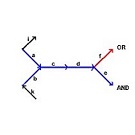
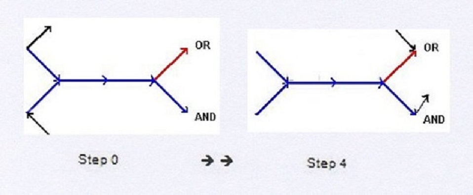
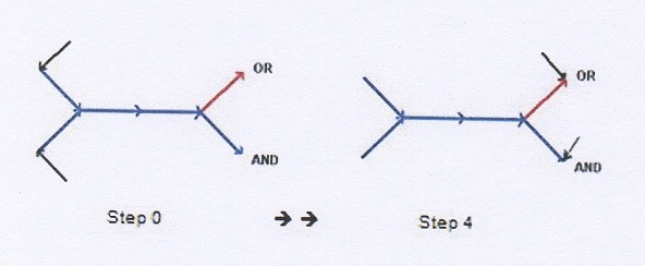
Figure 19 demonstrates the logic operations with the input TRUE AND/OR TRUE (at step 0) and the output at step 4 with the result TRUE for both OR and AND operations. The intermediate steps behave similarly to the corresponding steps of Figure 18.

Figure 19:

5.6.2 Configuration of NOT Gate

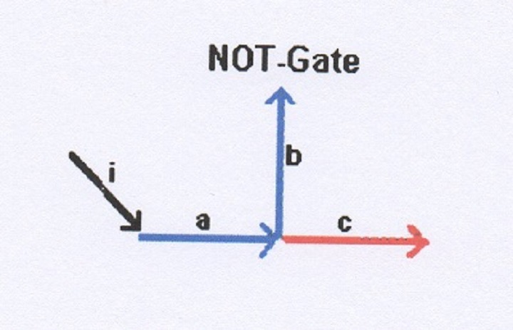
Figure 20 shows the configuration of a NOT gate. It consists of the conductor arcs $a$ and $b$, the filter arc $c$, and the information arc $i$.
The time steps evolve as follows (see Figure 21):

1. The information arc $i$ enters the end point of the conductor arc $a$.

2. Arc $i$ moves to the start point of $a$ (rule 2). The arc also meets the end points of $b$ and $c$.

3. Arc $i$ moves to the start point of arc $b$ (rule 2).

4. The start point of arc $b$ moves to the opposite point of arc $i$ (rule 3).

5. Arc $i$ moves back to the end point of $b$ and encounters the end point of the filter arc $c$ (rule 8).

Figure 20: Not-Gate

Figure 21:

5.7 Rule Example 7 - Copy Machine/Oscillator

The graph consists of three types of arcs:

• Several Type A arcs to be copied. These arcs have different properties and do not interact whith each other, except that the arcs are connected by an arc of Type C .

• A receiver arc of Type B .

• A transmitter arc of Type C .

5.7.1 Copy Machine

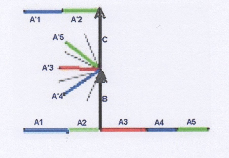
The foot of the Type B arc passes over a path consisting of Type A arcs to be copied (see Figure 22). The head of the Type B arc is connected to the foot of the Type C arc and a set of Type A arcs with different properties. The head of the Type C arc is connected to a path of Type A arcs already copied. If the foot of the Type B arc passes over a Type A arc to be copied, it transmits the properties of this arc to its head and activates an adjacent arc of Type A that has the same properties as that of the arc to be copied. The activated arc is transmitted from the foot of the Type C arc to its head. The path of the already copied arcs moves to the other end of the activated arc.

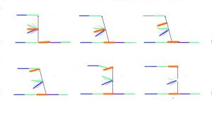
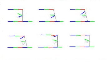
In Figure 23 at step 1, a red arc ($A_{3}$) is copied ($A\text{\textquoteright}_{3}$); at step 2 (Figure 24), a blue arc ($A_{4}$) is copied; and at step 3, a green arc ($A_{5}$) is copied. Intermediate steps show the movements from step to step.

Figure 22:

Figure 23: Step 1

Figure 24: Step2

5.7.2 Oscillator

The chain of type A arcs can build a loop. The result is then a chain of copied arcs, which repeate periodically.

5.8 Rule Example 8

The graph consists of four types of arcs:

• conductor arcs for transport of Type A, B, or C arcs (black)

• ABC arcsof Type A (red)

• ABC arcsof Type B (blue)

• ABC arcsof Type C (green)

Rules:

1. There is no interaction between arcs of the same type.

2. IF: The start point $ABC_{1}$ of an arc of type ABC is connected to a single conductor arc point $L_{i}$ that has no other conductor arc as neighbor
   THEN: With the next step, that start point $ABC_{1}$ will move to point $L_{k}$, which is the opposite of $L_{i}$ .

3. IF: The start point $ABC_{1}$ of an arc of type ABC is connected to two conductor arc points $L_{k}$ and $R_{l}$
   and if $ABC_{1}$ was previously connected to the conductor arc point $L_{i}$
   THEN: With the next step, that start point $ABC_{1}$ will move to point $R_{m}$, which is the opposite of $R_{l}$.

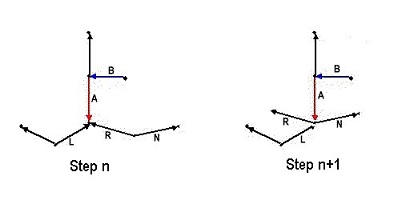
4. Attraction (see Figure 25)
   IF: The start point $A_{1}$ of the arc of type A was previously connected to the conductor arc point $L_{i}$ and is now connected to the opposite point $L_{k}$ and its neighbor $R_{m}$, and the end point $A_{0}$ of the arc of type A is connected to the start point $B_{1}$ of an arc of type B.
   THEN: With the next step, the start point $A_{1}$ will be connected to the points $L_{k}$ ,$R_{l}$ , and $N_{m}$, where $R_{l}$ is the opposite of $R_{m}$, and $N_{m}$ was previously connected to $R_{l}$ .

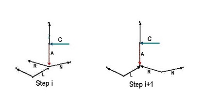
5. Repulsion (see Figure 26)
   IF: The start point $A_{1}$ of the arc of type A was previously connected to the conductor arc point $L_{i}$ and is now connected to the opposite point $L_{k}$ and its neighbors $R_{l}$ and $N_{m}$, and the end point $A_{0}$ of the arc of type A is connected to the start point $C_{1}$ of an arc of type C
   THEN: With the next step, the start point $A_{1}$ will be connected to the points $L_{k}$, and $R_{m}$ where $R_{m}$ is the opposite of $R_{l}$.

6. The rules regarding the arc types A, B, and C are also valid if either A is replaced by B, B is replaced by C, and C is replaced by A, or A is replaced by C, C is replaced by B, and B is replaced by A

Figure 25:

Figure 26:

Configuration 1

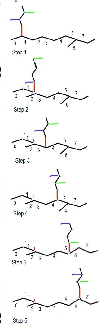
The graph shown in Figure 27 has two chains of conductor arcs:

• A horizontal chain of eight arcs with numbers from 0 to 7

• A vertical chain whose lowest arc is linked to the end point $A_{0}$ of an arc of type A

Step

1: The start point $A_{1}$ is linked to the arcs 0 and 1 at the left side of the horizontal chain. With the following steps, $A_{1}$ moves to the next arcs of the horizontal chains from left to right. The start points $B_{1}$ of an arc of type B and $C{}_{1}$ of an arc of type C are linked to arcs of the vertical chain, as shown in Figure 27.

Step

2: $A_{1}$ moves to the right. $C_{1}$ moves up to the end of the vertical chain. $B_{1}$ moves down to the bottom of the vertical chain and is now linked to the end point $A_{0}$ . Owing to this configuration, rule 4 is applicable. $A_{1}$ is then linked to the arcs 1, 2, and 3.

Step

3: $A_{1}$ moves to the right from arc 3 to arc 4. $B_{1}$ moves up and $C_{1}$ moves down according to rule 2.

Step

4: $A_{1}$ moves to the right from arc 4 to arc 5. $B_{1}$ moves up, and $C_{1}$ moves down according to rule 3.

Step

5: $A_{1}$ moves to the right from arc 5 to arc 6. $B_{1}$ moves up, and $C_{1}$ moves down according to rule 3. $B_{1}$ moves up to the end of the vertical chain. $C_{1}$ moves down to the bottom of the vertical chain and is now linked to the end point $A_{1}$. Owing to this configuration, rule 5 is applicable. $A_{1}$ is then linked to arcs 5 and 6.

Figure 27:

Configuration 2

The vertical chain of conductor arcs shown in Figure 27 consists of only three arcs. This chain can be extended by any number of conductor arcs.

Configuration 3

The configurations can be extended using additional chains in combination with ABC arcs. The end point $B_{0}$ (blue arc), for instance, can also be linked to a chain of conductor arcs. The start points of two arcs of types A and C are then connected to this chain. In this way, a nested system of conductor arcs and ABC arcs can be constructed.

Configuration 4

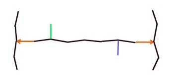
In Figure 27, the upper end of the vertical chain is not connected to any arc. In Figure 28, the horizontal chain with type A, B, and C arcs is terminated by type A arcs at both ends. Therefore, this chain will move on both sides along the vertical chains of conductor arcs at the same time. The type B and C arcs travel back and forth between the ends of the horizontal chain. The frequency of this commuting depends on the chain length.

Figure 28:

6 Signals, Information Arcs, ad Information Pulses

In Rule Example 6, the information TRUE or FALSE is represented as an information arc. As an alternative, the values $V(A_{0})/V(A_{1})$ can be used for transmitting an information pulse [the values $V(A_{0})$ and $V(A_{1})$ are assigned to the start and end points, respectively].

Let us consider the sequence of arcs $a$, $b$, and $c$, where $a_{1}$ meets $b_{0}$ and $b_{1}$ meets $c_{0}$. A signal (information pulse) starts at $a_{0}$ and propagates to $a_{1}=b_{0}$, then to $b_{1}=c_{0}$, and then to $c_{1}$ from step to step. According to cellular rules, the signal can change from step to step. With information pulses instead of information arcs, the configurations of the AND/OR gates (Example 6), and the Copy Machine (Example 7) can be constructed more simply.

The AND gate performs a logical AND operation on two logic inputs and produces a single logic output. The end points of the two conductor arcs $a$ and $b$ receive information pulses at $a_{0}$ and $b_{0}$. These pulses are propagated to their start points $a_{1}$ and $b_{1}$. The start points meet at the end point $c_{0}$ of the filter arc $c$. If both information values at the node {$a_{1},b_{1},c_{0}$} are TRUE, then a signal for TRUE is transmitted from the end point $c_{0}$ to the start point $c_{1}$. If one of the information values is FALSE, then a signal for FALSE is transmitted.

The Copy Machine copies the properties of the nodes of a chain with the arcs $a,b,c,d...$ to the nodes of a parallel chain with the arcs $a^{\prime}$, $b^{\prime},c^{\prime},d^{\prime}...$ In the start, a copier arc is linked to the endpoints $a_{0}$ and $a^{\prime}_{0}$, and transmits the value $V(a_{0})$ to $V(a^{\prime}_{0})$. Then, the copier arc moves to the start points of $a$ and $a^{\prime}$ and copies $V(a_{1})$ to $V(a^{\prime}_{1})$. With the next step, the copier arc moves to $b_{1}$ and $a^{\prime}_{1}$, and so forth. The abovementioned examples describe how information pulses can travel through a graph without changing the graph structure. Even more interesting, but also more complex, are systems in which the interaction of arcs can produce information pulses, which then trigger the interaction of arcs again.

7 Visualization

The pularity of CAs might be a consequence of the following facts:

• CA is often used to simulate natural or mathematical phenomena that can be mapped on a plane or space.

• The grid can be mapped onto any medium, such as paper, computer memory, or monitors.

• The grid has a uniform pattern, and the neighbors of a cell do not change their positions.

• The rules can be executed easily for each cell.

Visualizing XCA games is not as easy as visiualizing CA games, because the neighbors repeatedly change and their graphs are difficult to visualize. All graphs shown above are drawn manually in such a way that the graphs look rather intelligible. However, drawing very large graphs manually is nearly impossible. In general, there is no unique procedure for drawing a graph, nor is there a unique algorithm for visualizing a graph. For example, you can draw a graph by assigning to each vertex any arbitrary coordinate within a given frame. The result can then look rather chaotic. Drawing the graph more meaningfully requires adequate algorithms. An Internet search for “graph drawing” returns nearly one million matches, including many algorithms for graph visualization. For drawing the graph of the first time step of an XCA game, force-based algorithms (also known as force directed placement, or force directed layout algorithms) appeare to be the best choice [9].

Animations of the examples, shown above, are designed manually in such a way as to show how the graphs of consecutive time steps evolve. This is achieved by inserting intermediate steps, as was explained in Rule Example 2 using Figure 6.

8 Artificial World

Using an XCA, an artificial world can be simulated, beginning with a Big Bang.

According to the Big Bang theory, our universe began with a singularity. All energy was concentrated in one singular point. Space did not exist from the beginning. Since physical theories presupposes the existence of space, time, and matter, physical theories were not valid before the creation of space. How was space created after the Big Bang and what happened between the starting time and the time when space came into existence? Nobody knows, and imagining what happened is difficult.

There are many approaches to solving this mystery. The existence of Plank’s length and time indicates that space has a granular structure, rather than being a continuum. Some authors, such as Zirek[13] and Ostoma and Trushyk[12], have attempted to explain the Big Bang and the universe as a CA consisting of a huge array of cells capable of storing numeric information. They might be able to explain physical phenomena using CA. However, this approach presupposes the existence of a grid from the very beginning, and a grid is not a singularity.

Stephen Wolfram believes that space is a giant network of nodes[10][11]. It could work similarly to a so-called substitution system by which some node or substructure of the network could be replaced at each time step by another structure according to some fixed rule. The substitution system requires the neighborhood of the replaced structure, and the substitution remains unchanged.

With this assumption, the creation of a grid can be explained, starting from a singular node. However, only a planar grid can evolve in this system, and the network will grow endlessly.

I follow up on the idea that space is a giant network. However, I am considering the XCA model with which I am trying to explain the start of the universe and the creation of space by the evolution of a dynamic graph.

Many people, including me, believe that the universe is a giant computer system. The subject of this belief is known as digital physics.

Many different worlds can be created with the many possible XCA rules.

I am tempted to believe, that with XCA, it will be possible to simulate the physical world, provided that appropriate rules are found. This is not yet the case.

8.1 Space/Grid

Stephen Wolfram believes “that what is by far the most likely is that the lowest level space is a giant network of nodes”[10][11]. I also believe that a giant XCA graph (network) with appropriate rules and configuration can create its own space.

Graphs have properties similar to those of space, but unlike space, graphs are never continua. However, grid graphs (lattice graphs, tilings, tessellations) can be considered as a substitude for space. In contrast to CAs, an XCA does not require a grid, but it can create one, just as the real universe after the Big Bang generated its own space, which had not existed previously. Rule Examples 4 and 5 above demonstrate that the creation of grid graphs is possible. The grid can be a square grid or a cubic grid, but it can also be an irregular (or unstructured) grid. A planar graph can be considered as a two-dimensional irregular grid graph. In general, d-dimensional irregular grid graphs consist of d-dimensional cells bounded by (d -1)-dimensional faces. The cells and faces must not be intersected by any object.

8.2 Attraction/Repulsion

In the real world, the distance between objects can decrease or increase as a result of forces.

Let us consider an arc $a$ that is connected to the start points of the arcs $b$ and $c$. The distance between the end points of the arcs $b$ and $c$ is either two, if all arcs are neighbored, or three, if $b$ and $c$ are not neighbored. Transition from the constellation with a distance of two to the other constellation can be seen as repulsion, whereas the transition from distance three to distance two can be seen as attraction.

Figure 25 of Rule Example 5.8 demonstrates how attraction might work.

Figure 26 demonstrates how repulsion might work. The chain of conductor arcs with L and N is enlarged by the arc R. If the third arc R does not exist, then there is no enlargement. Normally, the balance between attraction and repulsion might be retained. However, if in some cases, the enlargement does not occur, then attraction will outweigh repulsion.

In reality, attraction outweighs repulsion through the gravitational force. The counter force of gravitation is the centrifugal force.

In the XCA world, the centrifugal force might be caused by a restriction rule to the effect that transitions must not allow reversing, which means that the status of two arcs at time step t +1 is the same as that time step t -1.

8.3 Virtual Dimension

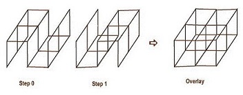
The considerations above apply to grids of a discrete time step. If we observe the evolution, over two or more steps, we might find that the dimension of a grid is higher than that of the grid per step. Example 1: We know that a complete graph with five nodes is not planar. If we discard one of the 10 arcs, then the graph is planar. Let us assume that with a next time step, another arc is removed from the complete graph. The graphs of both steps are planar. However, if we overlay the steps, the graphs look as if they are complete.

Example 2: The graphs of steps 0 and 1 In Figure 29 are planar, while the overlay of both graphs is a cubic grid.

Figure 29: Virtual Dimension

8.4 Time Aspects

8.4.1 Step-based Time

With an XCA, time can be measured by the number of steps, provided that the time between two steps is the same for all arcs, i.e., all arcs interact in a synchronized manner. However, what might happen if the arcs are not synchronized? Let us consider two neighboring arcs with different time steps. The arcs might then interact, for instance, according tothe following rule examples:

• The faster arc must wait until the slower one is ready.

• The active arc predicts the time of interaction.

• The arcs interact only when a signal arrives.

8.4.2 Event Time

If we compare two areas of a graph at a particular time span (number of steps), then we might find that one area has fewer transactions than the other. This could be interpreted such that the time in the first area is slower than that in the other one. In an extreme case, where no changes occur in the first area, time stands still.

8.4.3 Space Time

The length between two nodes can be measured by the number of arcs that build the path. However, this number changes from step to step. A better measurement of the distance between two nodes might be the shortest time that an arc or signal requires to travel from one node to the other one. Note, that with this definition, the distance measured from node $A$ to node $B$ is not necessarily identical with that measured from node $B$ to node $A$. Let us assume two nodes $A$ and $B$. Many different paths connect the nodes. At the start, many signals are spread from node $A$ over the system. The signals move randomly through any path, and some might arrive at node $B$ earlier or later. The first signal that arrives at B has then traversed the shortest path between $A$ and $B$ and determines the distance between $A$ and $B$. The shortest path of the next time step is not necessarily the same as that of the previous one.

8.5 Elementary Particles

The crucial statement of this hypothesis is that all phenomena, succh as space, radiation, and particles, originate from the different configurations and evolutions of subgraphs.

• Empty space, that is, an area free of radiation and particles, nevertheless, contains arcs. Because arcs are considered to have energy units, empty space aldo contains energy.

• A photon, emitted by a particle, moves with the highest speed to another particle, by which it is absorbed. The chains with type A, B and C arcs, as described in Chapter 5.8, might serve as a model of a hypothetical photon. The length of the chain defines the frequency. Both ends of the chain can move to different destinations.

• Elementary particles are more complex and have long lives. Interactions with the environment cannot destroy their identity. A hypothetical particle might consist of a kernel surrounded by a planar surface. Arcs of the surface are connected with arcs of the environment. However, there are no direct connections between the environment and the kernel. While the environment is a three-dimensional grid, the kernel is more complex and can consist of higher dimensions.

9 Conclusion

The examples with different rules show how manifold the concept of XCA is. However, in addition to the promising results, there are still open problems. Just as the Game of Life simulates birth, survival, and death, an XCA game can simulate a system that starts from a singularity, and evolves into a complex space. Although an example proves that this is possible, that example is not comparable with the versatility of the Life Game. No example of this article is shown with more than 16 arcs and 6 steps. Obtaining more meaningful results, requires more cells (arcs) over many time steps. This is true for both CAs and XCAs. As stated in Chapter 7, drawing very large graphs manually is nearly impossible. To explore the behavior of very large XCA systems over a huge number of steps, we need adequate programs, that calculate and visualize the consecutive steps. I would not have published this article before having such programs. However, I am more than 80 years (*1933) old, and I do not have much time left to come to a reasonable end. Now, it might be your turn to continue the game.

10 Acknowledgement

The author would like to thank Journal Prep (www.journalprep.com) for a peer review, and to thank Enago (www.enago.com) for the English language review.

Appendix A Appendix

A.1 Cellular Automaton

In 1970 John H. Conway published “The Game of Life” [1] that became soon very popular. This “game” is the best-known example of a cellular automaton [2] (CA). ‘The Game of Life (or simply Life) is not a game in the conventional sense. There are no players, and no winning or losing. Once the "pieces" are placed in the starting position, the rules determine everything that happens later’ [3]. ‘The "game" is a zero-player game, meaning that its evolution is determined by its initial state, requiring no further input from humans. One interacts with the Game of Life by creating an initial configuration and observing how it evolves.’ [4]

Life is an example of self-organization [5].

The different examples of the cellular automaton show how chaos may evolve into a structured organization.

See some examples on the site: http://www.collidoscope.com/modernca/ [6]. Before going into details, I am introducing the general concept of cellular automaton.

A CA consists of an n-dimensional grid, to the cells of which certain values are assigned at a definite time. For each next time step, the value of each cell changes according to the values of the neighboring cells (usually including the cell itself) and according to some transition rules.

As an example, the Game of Life acts on a two-dimensional rectangular grid. Each cell can be in one of two states; live or dead (represented by the values zero and one). A square cell has eight adjacent neighbors, four orthogonal and four diagonal cells. At each time step the following transitions occur simultaneously to every cell:

• A dead cell with exactly three live neighbors becomes a live cell (birth)

• A live cell with two or three live neighbors stays alive (survival)

• In all other cases, a cell dies or remains dead (overcrowding or loneliness)
  

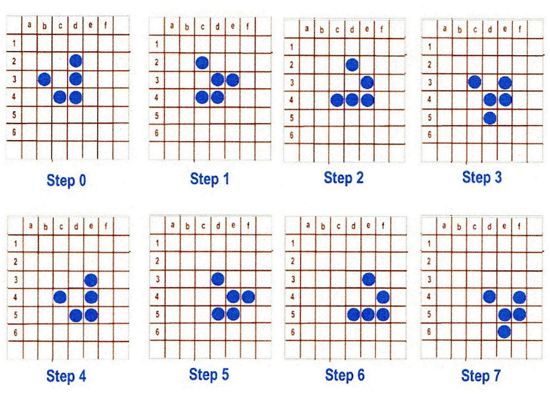
Figure 30 shows a so-called Glider. After every fourth step, the patterns are repeating. However, this patterns are shifted by one row and column, thus gliding diagonal from top left to bottom right. Let us see how the starting configuration of step 0 evolves to step 1.

1. All cells in 1st row: these cells have no three live cells; therefor remain dead

2. All cells in 1st column: these cells have no three live neighbors; therefor remain dead

3. Live cell on 2nd column (b), 3rd row (3): this cell has neither two nor three live neighbors; therefor gets dead

4. All dead cells in 2nd column remain dead because they have no three live neighbors

5. Dead cell on 3rd column (c), 2nd row (2): this cell has three neighbors; therefor gets alive

6. Dead cell on 3rd column (c), 3rd row (3): this cell has five neighbors; therefor remains dead

7. Live cell on 3rd column (c), 4th row (4): this cell has three live neighbors; therefor remains alive

8. Live cell on 4th column (d), 3rd row (3): this cell has only one neighbor; therefor gets dead

9. Live cell on 4th column (d), 4th row (4): this cell has two live neighbors; therefor remains alive

10. Dead cell on 5th column (e), 3rd row (3): this cell has three live neighbors; therefor gets alive

11. All remaining dead cells remain dead because they have no three live neighbors

Figure 30: Glider

You may find many sites about CA and the Game of Life on the World Wide Web [8].

Even if the game starts with chaotic condtitions, after a number of time steps different types of patterns may be seen:

• ‘still lives’ are patterns that do not change

• ‘oscillators’ repeat their status

• Sometimes patterns appear that seem to replicate themselves. The ‘glider’ shown in Figure3 is such a pattern

A.2 Adjacency Matrix, Incidence Matrix, Incidence List

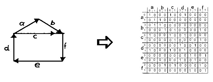
A graph can be described by an Adjacency Matrix. Normally, with the classical view, this matrix shows how the nodes are connected; when the entry at row, column is 1 in the matrix, the nodes are connected. With the XCA view, where arcs are seen as objects, the adjacency matrix represents which end points of arcs are adjacent to which other endpoints of arcs. The adjacency matrix on $n$ arcs is then a $2n\times 2n$ matrix, (or a $n\times n$ matrix, the elements of which are $2\times 2$ sub matrices). If the end point $a_{i}$ of arc $a$ meets the end point $b_{j}$ of arc $b$, then the entry of $a_{i}b_{j}$ is 1 else the entry is 0.

In Figure 31, for instance, the entry of $e_{1}d{}_{0}$ is 1.

Figure 31: Adjacency Matrix

Another matrix representation for a graph is the incidence matrix. This matrix is the same for both views.

The incidence matrix assigns each row to a node and each column to an edge. For a standard incidence matrix a 1 appears wherever a row’s node is incident on the column’s arc. The elements are zero otherwise.

The incidence matrix can be compressed to the incidents’ list: to each arc, the source and target node is assigned.

A.3 PSEUDO CODES OF THE BIG BANG GAME

The following pseudo codes do not reflect the performance problems. Since the matrix elements are ones and zeros, these values can be packed within bytes and may be considered as 2 x 2 sub matrices. The bits in a sub matrix can then be addressed as binary numbers.

For instance, the bit in the 2 x 2 sub matrix S[0][1] can be represented by the decimal number 0 x 1 + 1 x 2 + 0 x 4 + 0 x 8 = 2,

or S[1][0] by 0 x 1 + 0 x 2 + 1 x 4 + 0 x 8 = 4

A.3.1 BIG BANG GAME

⬇

//

//

//Input: Incidents List L, number of arcs n, number of nodes m,

// Property List P with properties assigned to arcs

// Rules R

// number of time steps nt

begin

read L,n,m,P,nt

for each step from 0 to nt

//Convert incidence list to adjacency matrix

call Incidence2Adjacency(L,A,n,m)

//Apply transition rules on adjacency matrix

call Transition(A,B,n,P,R)

//Convert adjacency matrix to incidence matrix

call Adjacency2Incidence(A,n)

//Convert incidents matrix to incidence list

call IncidentsMatrix2List(A,L,n,m)

Visualise the graph

end for

end

A.3.2 Transition

⬇

procedure Transition(A,B,n,P,R)

//Input: Adjacency Matrix A with n Arcs //first row and column are starting with index = 1

//Output: Matrix B

begin //1

row = 1

column = 2

for each row from 1 to n //2

for each column from 2 to n //3

calculate new value B[row][column]

according to the transition rules dependent on A[row][column]

end for //3 - column

end for //2 - row

return matrix B

end //1

A.3.3 CONVERT INCIDENCE LIST TO ADJACENCY MATRIX

⬇

procedure Incidence2Adjacency(L,A,n,m)

//Input:Incidents List with n arcs and m nodes

//first arc and node are starting with index = 1

//Output:Adjacency Matrix A.

Incidents List L(arc,source,target)

Incidents Matrix A

Node List NodeList[n][m]

SourceList[m][n]

TargetList[m][n]

begin //1

node = 0

for each arc in L from 1 to n //2

GetIncidentsList(arc,source,target)

SourceList[source][arc] = 1

TargetList[target][arc] = 1

end for //2

Create new matrix A[2][2][n][n]

for each node from 1 to m //3

arcsource = 0

arctarget = 0

for each arc from 1 to n //4

if SourceList[node][arc] is TRUE //5

then

if arcsource is 0

then

arcsource = arc

end if

end if //5

if TargetList[node][arc] is TRUE //6

then

if arctarget is 0

then

arctarget = arc

end if

end if //6

if arcsource < arctarget //7

then

arc_node = arcsource

sub_node = 0

else

arc_node = arctarget

sub_node = 1

end if

end for //7

//

if sub_node = 0

then

sub_alt = 1

else

sub_alt = 0

end for

for each arc from 1 to n //8

if SourceList[node][arc] is TRUE

then

SetAdj(A,n,sub_node,0,arc_node,arc,TRUE)

SetAdj(A,n,sub_alt, 1,arc,arc_node,TRUE)

end if

if TargetList[node][arc] is TRUE

then

SetAdj(A,n,sub_node,1,arc_node,arc,TRUE)

SetAdj(A,n,sub_alt ,0,arc,arc_node,TRUE)

end ifCONVERT INCIDENCE LIST TO ADJACENCY MATRIX

end for //8

end for //3

//Completion of the adjacency matrix

//If arc i is adjacent to j and arc arc j is adjacent to k

//then arc i is also adjacent to k

for each row from 1 to n //9

for each column from 1 to n //10

for each subrow from 0 to 1 //11

for each subcolumn from 0 to 1 //12

//

if GetAdj(A,n,subrow,subcolumn,row,column) is TRUE //13

then

for each row1 from 1 to n //14

for each subrow1 from 0 to 1 //15

if GetAdj(A,n,subrow1,subcolumn,row1,column) is TRUE //16

then

for each column1 from 1 to n //17

if GetAdj(A,n,subrow1,subcolumn,row1,column) is TRUE //18

then

SetAdj(A,n,subrow, subcolumn,row, column1,TRUE)

end if //18

end for //17 - column1

end if //16

end for //15 - subrow1

end for //14 - row1

end if //13 - GetAdj

//

end for //12

end for //11

end for //10

end for //9

end //1

A.3.4 CONVERT ADJACENCY MATRIX TO INCIDENCE MATRIX

⬇

procedure Adjacency2Incidence(A,n)

//Input: Ajacency Matrix A with n Arcs //first row and column are starting with index = 1

//Matrix A, converted to Incidents Matrix. Some of the 2 x n nodes are isolated

//Output: Incidence List: source and target nodes assigned to arc

//Enumerate subrows from 1 to 2 x n

//Enumerate subcolumns from 1 to n

//Assign adjacent end points to the next non empty subrow

//If A and B are adjacent and B and C are adjacent, then A is also adjacent to C, subsequently C is indirect adjacent to A

//Discard indirect adjacencies

//Because the matrix is symetric, matrix entries above the diagonal are processed only,

begin //1

row = 1

column = 2

for each row from 1 to n //2

for each column from 2 to n //3

for each subrow from 0 to 1 //4

for each subcolumn from 0 to 1 //5

if GetAdj(A,n,subrow,subcolumn,row,column) is TRUE //6

then

for each row1 from 1 to n //7

for each subrow1 from 0 to 1 //8

if GetAdj(A,n,subrow1,subcolumn,row1,column) is TRUE //9

then

for each column1 from 1 to n //10

if GetAdj(A,n,subrow1,subcolumn,row1,column) is TRUE //11

then

SetAdj(A,n,subrow1,subcolumn,row1,column1,FALSE)

//SetAdj(A,n,subrow, subcolumn,row, column1,TRUE)

end if //11

end for //10 - column1

end if //9

end for //8 - subrow1

end for //7 - row1

end if //6

end for //5 - subcolumn

end for //4 - subrow

end for //3 - column

end for //2 - row

return Incidence List

end //1

A.3.5 CONVERT INCIDENTS MATRIX TO INCIDENCE LIST

⬇

procedure IncidentsMatrix2List(A,L,n,m)

//Input: Incidents Matrix A with n Arcs and 2 x n nodes //first row and column are starting //with index = 1

//Output: Incidents List L(arc,source,target)

begin //1

NewNode = 0

//The two old nodes of arc y are 2 x y and 2 x y +1

//For getting the new nodes the non empty subrows are counted only

//In the NodeList(OldNode,NewNode,degree), OldNode is 2x(row-1)+subrow+1

//

//Count the degree of each OldNode

for each row from 1 to n //2

SetAdj(A,n,0,0,row,row,FALSE)

SetAdj(A,n,1,1,row,row,FALSE)

for each subrow from 0 to 1 //3

OldNode = 2x(row-1)+subrow+1

degree = 0

for each column from 1 to n //4

for each subcolumn from 0 to 1 //5

if GetAdj(A,n,subrow,subcolumn,row,column) is TRUE

then increment degree

end for //5

end for //4

end for //3

if degree > 0 //6

then

increment NewNode

SetNodeList[OldNode,NewNode,degree]

if degree is equal to 1 //7

then

SetAdj(A,n,0,0,row,row,TRUE)

SetAdj(A,n,1,1,row,row,TRUE)

end if //7

else

SetNodeList[OldNode,0,0]

end if //6

end if //2

//Build the Incidents List

OldNode = 0

for each column from 1 to n //11

source = 0

target = 0

for each row from 1 to n //12

for each subrow from 0 to 1 //13

increment OldNode

for each subcolumn from 0 to 2 //14

if GetAdj(A,n,subrow,subcolumn,row,column) is TRUE //15

then

node = GetNodeList(OldNode,NewNode)

if subcolumn is equal 0

then source = node

else target = node

end if //15

end for //14

end for //13

end for //12

if source > 0 and column > 0 //16

then

SetIncidentsList(column,source,target)

end if //16

end for //11

end //1