Online Metric-Weighted Linear Representations for Robust Visual Tracking
Abstract
In this paper, we propose a visual tracker based on a metric-weighted linear representation of appearance. In order to capture the interdependence of different feature dimensions, we develop two online distance metric learning methods using proximity comparison information and structured output learning. The learned metric is then incorporated into a linear representation of appearance. We show that online distance metric learning significantly improves the robustness of the tracker, especially on those sequences exhibiting drastic appearance changes. In order to bound growth in the number of training samples, we design a time-weighted reservoir sampling method.
Moreover, we enable our tracker to automatically perform object identification during the process of object tracking, by introducing a collection of static template samples belonging to several object classes of interest. Object identification results for an entire video sequence are achieved by systematically combining the tracking information and visual recognition at each frame. Experimental results on challenging video sequences demonstrate the effectiveness of the method for both inter-frame tracking and object identification.
Index Terms:
Visual tracking, linear representation, structured metric learning, reservoir samplingI Introduction
Visual tracking is an important and challenging problem in computer vision, with widespread application domains. Its goal is to consistently locate an object of interest in multiple images captured at successive time steps. Despite great progress in recent years, visual tracking remains a challenging problem because of the complicated appearance changes caused by factors including illumination variation, shape deformation, occlusion, pose variation, background clutter, sophisticated object motion, and scene blurring. To address these factors, a variety of tracking approaches have been proposed to improve the robustness, speed, or accuracy of visual tracking. In order to effectively capture the dynamic spatio-temporal information on object appearance, these tracking approaches aim to learn generative or discriminative appearance models using a variety of statistical learning techniques, including hidden Markov model [1], mixture models [2], subspace learning [3, 4, 5], linear regression [6, 7, 5, 8], covariance learning [9], compressive tracking [10], SVMs [11, 12, 13, 14], boosting [15, 16], random forest [17], spatial attention learning [18], metric learning [19, 20], and tracking-learning-detection [21].
Linear representations, in which the object is represented as a linear combination of basis samples, are often used to build such appearance models. Suppose that we have a set of basis samples denoted as: . Using these basis samples, a new sample y can be approximated by the following linear combination: , where is a coefficient vector. This gives rise to the following reconstruction error norm: . In this case, the smaller is, the more likely y is generated from the subspace spanned by . During visual tracking, the subspace is likely to vary dynamically as new data arrive, so should be accordingly adjusted to the new data. In addition, the feature representation for each sample is typically extracted from local image patches, whose appearance is often correlated because of their spatial proximity. Therefore, the elements of the feature representation in different dimensions often contain intrinsic spatial correlation information. In general, such correlation information is stable in the case of complicated appearance changes (e.g., partial occlusion, illumination variation, and shape deformation), and thus plays an important role in robust visual tracking. However, most existing linear representation-based trackers (e.g., [6, 7]) build linear regressors that treat feature dimensions independently and ignore the correlation between them.
Therefore, we address the following three key issues for tracking robustness and efficiency: i) how to capture the intrinsic correlation between different feature dimensions; ii) how to maintain and update a limited-sized basis sample buffer that effectively adapts during tracking; and iii) given this correlation information and a dynamically changing basis , how to efficiently compute the optimal coefficient vector c at each frame.
The core of our approach to these problems is online metric learning, which learns and updates a distance metric matrix over time. Within this framework, the three issues listed above are solved as follows. For i), inter-dimensional correlation is captured by the learned Mahalanobis distance metric matrix such that , where projects the feature vector to a more discriminative feature space. In other words, online metric learning aims to find a linear mapping (i.e., a set of linear combinations over the correlated feature elements from different feature dimensions), which projects the original samples to a more discriminative feature space for robust visual tracking. We compare two different metric learning methods, one of which uses structured learning while the other is based only on pairwise sample proximity. For ii), we design a time-weighted reservoir sampling method to maintain and update limited-sized sample buffers in the metric learning procedure. In addition, we prove that metric learning based on our reservoir sampling method is statistically close to metric learning using all observed training samples. For iii), we pose the calculation of c as a least-square optimization problem, which admits an extremely simple and efficient closed-form solution. We also demonstrate that, with the emergence of new data, the solution can be efficiently updated by a sequence of simple matrix operations.
Therefore, the main contributions of this work are two-fold: 1) We propose a novel online metric-weighted linear representation for visual tracking. The linear representation is associated with a metric-weighted least-square optimization problem, which admits an extremely simple and efficient closed-form solution. The metric used in the linear representation is updated online in a max-margin optimization framework using proximity comparison or structured learning. Different from the similarity metric learning developed in [22], our work is formulated as a max-margin optimization problem for learning a Mahalanobis distance metric. Furthermore, we introduce the idea of structured learning to the online metric learning process, which is also novel in the visual tracking literature. 2) We design a time-weighted reservoir sampling method to maintain and update limited-sized sample buffers in the linear representation. The method is able to effectively maintain sample buffers that not only retain some old samples to avoid tracker drift, but also adapt to recent changes. In addition, we theoretically prove that metric learning based on our reservoir sampling method is statistically close to metric learning using all available training samples. This is the first time that reservoir sampling is used in an online metric learning setting that is tailored for robust visual tracking.
We note that, if the template samples all represent the same object, this same procedure can be used to identify the object in the presence of multiple objects. The goal of object identification is naturally achieved by combining the tracking information and the linear regression-based visual recognition together. We obtain promising results of pedestrian identification on multi-view video sequences.
Compared to previous systems, we fully exploit the linear representation of object appearance in a consistent and principled manner. By using online metric learning, our similarity measure is better maintained despite changing conditions. Reservoir sampling allows us to represent object appearance over time as a linear combination of samples. Our incremental solution update allows rapid update of object appearance coefficients, either for object tracking or identification.
II Related work
Our work builds on recent progress in several related fields: i) linear representations; ii) distance metric learning; iii) reservoir sampling; and iv) structured tracking. We give a brief overview of the most relevant work in each of these areas.
Linear representations Mei and Ling [6] propose a tracker based on a sparse linear representation obtained by solving an -regularized minimization problem. With the sparsity constraint, this tracker can adaptively select a small number of relevant templates to optimally approximate the given test samples. The main limitation is its computational expense due to solving an -norm convex problem. To speed up the tracking, Bao et al. [23] take advantage of a fast numerical solver called accelerated proximal gradient, which solves the -regularized minimization problem with guaranteed quadratic convergence. An alternative is to solve the -regularized minimization problem in an approximate way. For example, Li et al. [7] propose to approximately solve the sparse optimization problem using orthogonal matching pursuit (OMP). Recently, research has revealed that the -norm induced sparsity does not necessarily help improve the accuracy of image classification; and non-sparse representations are typically orders of magnitude faster to compute than their sparse counterparts, with competitive accuracy [24, 25]. Subsequently, Li et al. [26] propose a 3D discrete cosine transform based multilinear representation for visual tracking. The representation models the spatio-temporal properties of object appearance from the perspective of signal compression and reconstruction. However, the above trackers construct linear regressors that are defined on independent feature dimensions (mutually independent raw pixels in both [6] and [7]). In other words, the correlation information between different feature dimensions is not exploited. Such correlation information can play an important role in robust visual tracking.
Distance metric learning The goal of distance metric learning is to seek an effective and discriminative metric space, where both intra-class compactness and inter-class separability are maximized. In general, distance metric learning [27, 28, 29, 30] is a popular and powerful tool for many applications. For example, in [27], a Mahalanobis distance metric is learned using positive semidefinite programming. Chechik et al. [22] propose a cosine similarity metric learning method using proximity comparison for large-scale image retrieval. Discriminative metric learning has also been successfully applied to visual tracking [19, 31, 20]. These works learn a distance metric mainly for object matching across adjacent frames, and the tracking is not carried out in the framework of linear representations. In addition, Hong et al. [32] learn a discriminative distance metric in a max-margin framework, where the average inter-class distance is maximized while minimizing the average intra-class distance. The distance metric learning approach is implemented in a batch mode learning scheme, which does not allow for online updating required for visual tracking.
Reservoir sampling Visual tracking is a time-varying process which deals with a dynamic stream data in an online manner. Due to memory limitations, it is often impractical for trackers to store all the video stream data. To address this issue, reservoir sampling is a means of maintaining and updating limited-sized data buffers. However, the conventional reservoir sampling in [33, 34] can only accomplish the task of uniform random sampling, which assumes all samples are equally important. Due to temporal coherence, visual tracking in the current frame usually relies more on recently received samples than old samples. Hence, time-weighted reservoir sampling is required for robust visual tracking.
Structured tracking The objective of structured tracking is to utilize the intrinsic structural information on object appearance for robust object tracking. For instance, Jia et al. [35] construct a structured sparse appearance model, which performs alignment pooling on the sparse coefficient vectors for local patches within the object. Similar to [35], Zhong et al. [36] also propose a structured appearance model that carries out average pooling on the sparse coefficient vectors for local image patches within the object. Likewise, Li et al. [37] present a local block-division appearance model that comprises a set of block-specific SVM classification models. The Dempster-Shafer evidence theory is further used to fuse the block-specific SVM discriminative information for object localization. In addition, structured output learning (e.g., structured SVM [13]) is applied to visual tracking. Its key idea is to learn a classification model in a max-margin optimization framework, which involves an infinite number of constraints containing structured information (e.g., VOC overlap score [13]).
Tracking and identification Recent studies have demonstrated the effectiveness of combining object identification and tracking together. For example, Edwards et al. [38] present an adaptive framework that improves the performance of face tracking and recognition by adaptively combining the motion information from the video sequence. Following this work, Zhou et al. [39] study the problem of simultaneous tracking and recognizing human faces in a particle filter framework. Moreover, Mei and Ling [6] formulate simultaneous vehicle tracking and identification as a -regularized sparse representation problem.
Compared with the previous work on appearance modeling, the advantages of this work are as follows. First, this work constructs a simple but effective appearance model based on a metric-weighted linear regression problem, which admits an extremely simple and efficient closed-form solution with online updating. Second, this work naturally embeds useful discriminative information within the process of appearance modeling using online metric learning, which finds an effective metric space (obtained by discriminative linear mappings) for metric-weighted linear regression. Third, this work effectively maintains limited-sized sample buffers for online metric learning by time-weighted reservoir sampling. The maintained buffers can not only retain some old samples with a long lifespan for avoiding the tracker drift, but also adapt to recent appearance changes. A preliminary conference version of this work appears in [40].
III The proposed visual tracking algorithm
III-A Particle filtering for tracking
At the top level, visual tracking is posed as a sequential object state estimation problem, which is often solved in a particle filtering framework [41]. The particle filter can be divided into prediction and update steps:
where are observation variables, and denotes the motion parameters including translation, translation, and scaling. The key distributions are denoting the observation model, and representing the state transition model. Usually, the motion between two consecutive frames is assumed to conform to a Gaussian distribution: , where denotes a diagonal covariance matrix with diagonal elements: , , and . For each state , there is a corresponding image region that is normalized by image scaling. The optimal object state at time can be determined by solving the following maximum a posterior (MAP) problem: . Therefore, efficiently constructing an effective observation model plays a critical role in robust visual tracking. Motivated by this observation, we design a metric-weighted linear representation that captures the intrinsic object appearance properties in a discriminative distance metric space.
III-B Problem formulation
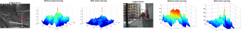
Modeling the observed appearance of an object is more complex than modelling its motion. This is often posed as a problem of linear representation and reconstruction, which corresponds to a -norm regularized least-square optimization problem (e.g., solved in [6, 7]). These optimization problems usually ignore the relative importance of individual feature dimensions as well as the correlation between feature dimensions. During tracking, such information plays a critical role in robust object/non-object classification with complicated appearance variations. Motivated by this observation, we propose a metric-weighted linear representation that is capable of capturing the varying correlation information between feature dimensions. As shown in Fig. 1, metric learning results in a linear representation that is more discriminative for object/non-object classification.
Metric-weighted linear representation. More specifically, given a set of basis samples and a test sample , we aim to discover a linear combination of to optimally approximate the test sample by solving the following optimization problem:
| (1) |
where and is a symmetric distance metric matrix that can be decomposed as . In principle, the idea of the metric-weighted linear representation is to linearly reconstruct the given test sample using the basis samples within a distance metric space (characterized by the Mahalanobis metric matrix ). The aforementioned linear regression problem is equivalent to the following form: . In other words, we perform the linear reconstruction task on the transformed sample with respect to the transformed basis samples . When is an identity matrix, our metric-weighted regression problem degenerates to a standard least square regression problem.
The optimization problem (1) has an analytical solution that can be computed as:
| (2) |
If is a singular matrix, we use its pseudoinverse to compute .
Tracking application. During tracking, we typically want to classify a candidate sample as either foreground or background. We are therefore interested in the relative similarity of the sample to a set of foreground and background samples. To address this problem, we obtain the foreground and background linear regression solutions as follows: and , where and are foreground and background basis samples, respectively.
Thus, we can define a discriminative criterion for measuring the similarity of the test sample to the foreground class:
| (3) |
where and are two scaling factors, = , , is a trade-off control factor, and is the sigmoid function. Here, the term reflects the reconstruction similarity relative to the foreground class, while determines the similarity with the background class. Greater with a smaller indicates a stronger confidence for foreground prediction.
During tracking, the similarity score is associated with the observation model of the particle filter such that .
Implementing this framework involves three main challenges: i) maintaining a representative pool of foreground and background samples; ii) efficiently updating the solution when foreground or background samples are updated; iii) learning and updating the metric matrix . These are addressed in the following four sections.
Input:
The current distance metric matrix , the basis samples , any test sample .
Output:
The optimal linear representation solution of sample .
-
1.
Build the optimization problem in Equ. (1):
-
2.
Compute the optimal solution . If samples are added to or removed from , can be efficiently updated in an online manner:
-
3.
Return the optimal solution .
III-C Online solution update
The main computational time of Equ. (2) is spent on the calculation of . For computational efficiency, we need to incrementally or decrementally update the inverse when a sample is added to or removed from , for a fixed metric . Motivated by this observation, we design an online update scheme that deals with the following three cases: 1) the basis sample matrix is incrementally expanded by one column such that ; 2) the basis sample matrix is decrementally reduced by one column such that is the reduced matrix after removing the -th column of ; and 3) one column of is replaced by a new sample.
Incremental case. Let denote the expanded matrix of . Clearly, the following relation holds:
For simplicity, let , , and . Since is a symmetric matrix, . The inverse of can be computed as [42]:
| (4) |
Decremental case. Let denote the reduced matrix of after removing the -th column such that . Based on [42], the inverse of can be computed as:
| (5) |
where stands for the index set except .
Replacement case. For adapting to object appearance changes, it is necessary for trackers to replace an old sample from the buffer with a new sample. Sample replacement is implemented in two stages: 1) old sample removal; and 2) new sample addition, corresponding to the decremental and incremental cases described above.
The complete optimization procedure including online sample update is summarized in Algorithm 1.
Input:
The current distance metric matrix and a new triplet .
Output:
The updated distance metric matrix .
-
1.
Calculate and
-
2.
Compute the optimal step length with .
-
3.
.
Input:
The current distance metric matrix , the current tracking bounding box and its associated feature vector .
Output:
The updated distance metric matrix .
-
1.
Most violated constraint set
-
2.
Sample a number of bounding boxes around to construct a constraint set for the optimization problem (14).
-
3.
Compute the most violated constraint as shown in Equ. (15).
-
4.
Add to the most violated constraint set such that .
-
5.
Solve the optimization problem (18) to obtain the optimal step length vector .
-
6.
Compute the updated metric matrix according to Sec. III-D.
-
7.
Repeat Steps 3–6 until convergence (restricted by a maximum iteration number).
-
8.
Return .
III-D Online proximity based metric learning
Having introduced the metric-weighted linear representation in Sec. III-B, we now address the key issue of calculating the metric matrix . should ideally be learned from the visual data, and should be dynamically updated as conditions change throughout a video sequence.
III-D1 Triplet-based ranking loss
Suppose that we have a set of sample triplets with . These triplets encode the proximity comparison information. In each triplet, the distance between and should be smaller than the distance between and .
The Mahalanobis distance under metric is defined as:
| (6) |
Clearly, must be a symmetric and positive semidefinite matrix. It is equivalent to learn a projection matrix such that . In practice, we generate the triplets set as: and belong to the same class and and belong to different classes. So we want the constraints to be satisfied as well as possible. By putting it into a large-margin learning framework, and using the soft-margin hinge loss, the loss function for each triplet is:
| (7) |
III-D2 Large-margin metric learning
To obtain the optimal distance metric matrix , we need to minimize the global loss that takes the sum of hinge losses (7) over all possible triplets from the training set:
| (8) |
where is the triplet set. To sequentially optimize the above objective function in an online fashion, we design an iterative algorithm to solve the following convex problem:
| (9) |
where denotes the Frobenius norm, is a slack variable, and is a positive factor controlling the trade-off between the smoothness term and the loss term . Following the passive-aggressive mechanism used in [22, 43], we only update the metric matrix when .
III-D3 Optimization of
We optimize the function in Equ. (9) with Lagrangian regularization:
| (10) |
where and are Lagrange multipliers. The optimization procedure is carried out in the following two alternating steps.
-
•
Update . By setting , we arrive at the update rule
(11) where and , .
-
•
Update . Subsequently, we take the derivative of the Lagrangian (10) w.r.t. and set it to zero, leading to the update rule:
(12)
The full derivation of each step can be found in the supplementary file (as shown in Sec. VII). The complete procedure of online distance metric learning is summarized in Algorithm 2.
III-D4 Online matrix inverse update
When updated according to Algorithm 2, is modified by rank-one additions such that where and are two vectors (defined in Equ. (11)) for triplet construction, and is a step-size factor (defined in Equ. (12)). As a result, the original becomes . When is modified by a rank-one addition, the inverse of can be updated according to the theory of [44, 45]:
| (13) |
Here, , (or ), and (or ).
III-E Online structured metric learning
Metric learning based on sample proximity comparisons leads to an efficient online learning algorithm, but requires pre-defined sets of positive and negative samples. In tracking, these usually correspond to target/non-target image patches. The boundary between these classes typically occurs where sample overlap with the target drops below a threshold, but this can be difficult to evaluate exactly and thus introduces some noise into the algorithm.
In this Section, we replace the proximity based metric learning module with an online structured metric learning method for learning . The main advantage of this method is that it directly learns the metric from measured sample overlap, and therefore does not require the separation of samples into positive and negative classes.
Structured ranking Let and denote two feature vectors extracted from two image patches, which are respectively associated with two bounding boxes and from frame . Without loss of generality, let us assume that corresponds to the bounding box obtained by the current tracker while is associated with a bounding box from the area surrounding . As in [13], the structural affinity relationship between and is captured by the following overlap function: As a result, we define the following optimization problem for structured metric learning:
| (14) |
where and . Clearly, the number of constraints in the optimization problem (14) is exponentially large or even infinite, making it difficult to optimize. Our approach to this optimization problem differs from [13] in four main aspects: i) our approach aims to learn a distance metric while [13] seeks a SVM classifier; ii) we optimize an online max-margin objective function while [13] solves a batch-mode optimization problem; iii) our optimization problem involves nonlinear constraints on triplet-based Mahalanobis distance differences, while the optimization problem in [13] comprises linear constraints on doublet-based SVM classification score differences; and iv) our approach directly solves the primal optimization problem while [13] optimizes the dual problem.
Structured optimization Inspired by the cutting-plane method, we iteratively construct a constraint set (denoted as ) containing the most violated constraints for the optimization problem (14). In our case, the most violated constraint is selected according to the following criterion:
| (15) |
For notational simplicity, let denote the loss term . Note that the violated constraints generated from (15) are used if and only if is greater than zero. Subsequently, we add the most violated constraint to the optimization problem (14) in an iterative manner, that is, . The corresponding Lagrangian is formulated as:
| (16) |
where and are Lagrange multipliers. The optimization procedure is once again carried out in two alternating steps:
-
•
Update . By setting to zero, we obtain an updated defined as:
(17) where , and denotes .
-
•
Update . To obtain the optimal solution for all Lagrange multipliers , we set for all , leading to the following optimization problem:
(18) where where , with being , and with being .
As before, the optimal is updated as a sequence of rank-one additions: . As a result, the original becomes . When is modified by a rank-one addition, the inverse of can again be updated according to the theory of [44, 45].
Algorithm 3 outlines the procedure of online structured metric learning. The complete derivation of these results is given in the supplementary file (as shown in Sec. VIII).
III-F Time-weighted reservoir sampling
In order to construct a metric-weighted linear representation (referred to in Equ. (1)) for visual tracking, we need to learn a discriminative Mahalanobis metric matrix by minimizing the total ranking losses (referred to in Equ. (8)) over a set of training triplets , which are generated from the training data (collected incrementally frame by frame) by proximity comparison. As tracking proceeds, the amount of collected training data increases, which leads to an exponential growth of the triplet set size (i.e., ). As a result, the optimization required for metric learning (referred to in Equ. (8)) becomes computationally intractable. To address this issue, a practical solution is to maintain a limited-sized buffer to store only selected training triplets. However, using the training triplets from the limited-sized buffer (instead of all training data) for metric learning usually leads to discriminative information loss. Therefore, how to effectively reduce such information loss is our focus in this work.
Inspired by the idea of reservoir sampling [33, 34, 46, 47] (i.e., sequential random sampling for statistical learning), we propose a sampling scheme to maintain and update the limited-sized buffer while preserving the discriminative information on the ranking losses as much as possible. Moreover, since the training data for tracking have to be collected frame by frame, the limited-sized buffer needs to be updated sequentially. Therefore, we seek a sequential sampling mechanism to online maintain and update the buffer, in such a way that the ranking losses for metric learning is as close as possible to those using all the received training samples. Reservoir sampling is one approach to this problem.
The classical version of reservoir sampling simulates the process of uniform random sampling [33, 34] from a large population of sequential samples. However, this is inappropriate for visual tracking because the samples are dynamically distributed as time progresses. Usually, recent samples should have a greater influence on the current tracking process than those appearing a long time ago. Therefore, larger weights should be assigned to recent samples while smaller weights should be attached to old samples. Based on weighted reservoir sampling [46, 47], our sample scheme further takes into account the time-varying properties of visual tracking, by incorporating time-related weight information into the weighted reservoir sampling process.
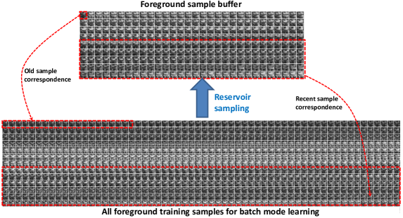
More specifically, we design a time-weighted reservoir sampling (TWRS) method for randomly drawing samples according to their time-varying properties, as listed in Algorithm 4. In the algorithm, each new sample is associated with a time-related weight with being the frame index number corresponding to and being fixed. Using this time-related weight, a random key for indexing the new sample is generated by with . After that, a weighted sampling procedure [47] is adopted to update the existing foreground or background sample buffer. Fig. 2 gives an intuitive illustration of the way that TWRS retains useful old samples while keeping sample adaptability to recent changes. Note that it is the first time that time-weighted reservoir sampling is used for visual tracking.
As described in the supplementary file, Theorem IX.1 states the relationship between the ranking losses respectively from the reservoir sampling-based buffer and all training data seen to date. This theorem shows that the sum of the ranking losses over the foreground and background buffers is probabilistically close to the sum of the empirical ranking losses over all the received training data.
Therefore, statistical learning based on our reservoir sampling method with limited-sized sample buffers can effectively approximate statistical learning using all the received training samples. In our case, reservoir sampling is used to maintain and update the foreground and background basis samples for discriminative distance metric learning. Hence, the TWRS method extends the reservoir sampling method [47] to cope with the online metric learning problem using two sample buffers. It is a version of reservoir sampling tailored for online triplet-based metric learning during visual tracking.
The key benefit of TWRS is to effectively generate and maintain the limited-sized sample buffers, which encourage the recent samples and meanwhile retain some old samples with a long lifespan. In this way, online metric learning using the limited-sized sample buffers approximates that of batch-mode learning (i.e., retaining all the samples during tracking), which balances the effectiveness and efficiency. The key difference from other online approaches (e.g., using forgetting factors) is that the total learning costs for TWRS are derived from the sequentially generated limited-sized sample buffers (retaining the old and recent samples simultaneously). In contrast, the online learning approaches using forgetting factors only store the recent samples and discard the previously generated samples. The costs of using the previously generated samples decay recursively using a forgetting factor. As a result, the online learning approaches using forgetting factors may suffer from the model drift problem.
Input:
Current buffers and together with their corresponding keys, a new training sample , maximum buffer size , time-weighted factor .
Output:
Updated buffers and together with their corresponding keys.
-
1.
Obtain the samples and with the smallest keys and from and , respectively.
-
2.
Compute the time-related weight with being the corresponding frame index number of .
-
3.
Calculate a key where .
-
4.
Case: foreground. If , ; otherwise, is replaced with when .
Case: background. If , ; otherwise, is replaced with when . -
5.
Return and together with their corresponding keys.
IV Experimental evaluation of our baseline tracker
IV-A Experimental configurations
1) Implementation details. For the sake of computational efficiency, we simply consider the object state information in 2D translation and scaling in the particle filtering module, where the corresponding variance parameters are set to (10, 10, 0.1). The number of particles is set to 200. In practice, the video sequences used for experiments consists of the targets with relatively slow motion and progressive scale variation in most cases. As a result, such settings for particle number and translational variances are adequate for robust visual tracking. Of course, in the case of fast motion or drastic object motion the parameter settings with larger variance parameters or more particles should be adopted. For each particle, there is a corresponding image region represented as a HOG feature descriptor ([48]) with cells (each cell is represented by a 9-dimensional histogram vector) in the five spatial block-division modes ( [49]), resulting in a 405-dimensional feature vector for the image region. The number of triplets used for online metric learning is chosen as 500. The maximum buffer size and time-weighted factor in Algorithm 4 is set as 300 and 1.6, respectively. Similarly to [16], we take a spatial distance-based strategy for training sample selection. The scaling factors and in Equ. (3) are chosen as 1. The trade-off control factor in Equ. (3) is set as 0.1. Note that the aforementioned parameters are fixed throughout all the experiments. If the proposed tracker is implemented in Matlab on a workstation with an Intel Core 2 Duo 2.66GHz processor and 3.24G RAM, the average running time of the proposed tracker is about 0.55 second per frame (because of the slow for-loop operations in Matlab). In contrast, if the proposed tracker is carried out in C++ with multi-thread parallel computation (for greatly speeding up the for-loop operations), the running time will be greatly reduced (for about 0.08 second per frame).


(a) (b) (c) (d)
2) Datasets and evaluation criteria A set of experiments are conducted on eighteen challenging video sequences, which consist of 8-bit grayscale images. These video sequences are captured from different scenes, and contain different types of object motion events (e.g., human walking and car running), which are illustrated in the supplementary file. For quantitative performance comparison, two popular evaluation criteria are introduced, namely, center location error (CLE) and VOC overlap ratio (VOR) between the predicted bounding box and ground truth bounding box such that . If the VOC overlap ratio is larger than , then tracking is considered successful in that frame.
IV-B Empirical analysis of parameter settings
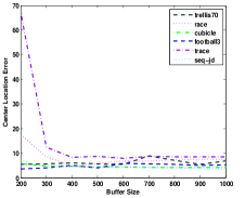
1) Sample buffer size. To test the effect of buffer size on reservoir sampling, we compute the average CLE and VOR for each video sequence using nine different sample buffer sizes. Figs. 3 (a) and (b) show the quantitative CLE and VOR performance on five video sequences. It is clear that the average CLE (VOR) decreases (increases) as the buffer size increases, and plateaus with approximately more than 300 samples.
2) Number of particles. In general, more particles enable visual trackers to locate the object more accurately, but lead to a higher computational cost. Thus, it is crucial for visual trackers to keep a good balance between accuracy and efficiency using a moderate number of particles. Fig. 3 (c) shows the average VOC success rates (i.e., ) of the proposed tracking algorithm on three video sequences. From Fig. 3 (c), we can see that the success rate rapidly grows with increasing particle number and then converges at approximately 200-300 particles for each sequence. Fig. 3 (d) displays the average CPU time (spent by the proposed tracking algorithm in each frame) with different particle numbers. It is observed from Fig. 3 (d) that the average CPU time slowly increase.
3) Comparison of different linear representations. The objective of this task is to evaluate the performance of four linear representations: our linear representation with metric learning, our linear representation without metric learning, compressive sensing linear representation [7], and -regularized linear representation [6]. For a fair comparison, we utilize the raw pixel features as in [7, 6]. Tab. I shows the average performance of these four linear representations in CLE, VOR, and success rate on four video sequences. Clearly, our linear representation with metric learning consistently achieves better tracking results than the three other linear representations. Please see the supplementary file for the details of the frame-by-frame tracking results (i.e., CLE, VOR, success rate).
4) Evaluation of different sampling methods. Here, we examine the performance of two sampling methods: uniform [33] and time-weighted [47] reservoir sampling. Tab. II shows the experimental results of the two sampling methods in CLE, VOR, and success rate on five video sequences. From Tab. II, we can see that weighted reservoir sampling performs better than ordinary reservoir sampling. More results of these two sampling methods can be found in the supplementary file.


| CLE | VOR | Success Rate | ||||||||||||||||
|---|---|---|---|---|---|---|---|---|---|---|---|---|---|---|---|---|---|---|
| trellis70 | race | cubicle | football3 | trace | seq-jd | trellis70 | race | cubicle | football3 | trace | seq-jd | trellis70 | race | cubicle | football3 | trace | seq-jd | |
| Ours+pixels with metric | 20.91 | 5.18 | 21.12 | 9.47 | 22.88 | 8.67 | 0.49 | 0.79 | 0.54 | 0.55 | 0.37 | 0.58 | 0.53 | 0.99 | 0.69 | 0.55 | 0.28 | 0.70 |
| Ours+pixels without metric | 66.32 | 7.91 | 40.48 | 14.83 | 139.30 | 20.59 | 0.27 | 0.67 | 0.18 | 0.46 | 0.07 | 0.51 | 0.30 | 0.89 | 0.25 | 0.28 | 0.08 | 0.62 |
| CS+pixels | 68.45 | 5.51 | 31.00 | 53.56 | 78.98 | 39.75 | 0.19 | 0.68 | 0.37 | 0.22 | 0.17 | 0.17 | 0.19 | 0.90 | 0.47 | 0.24 | 0.09 | 0.11 |
| L1+pixels | 27.64 | 160.79 | 24.26 | 64.07 | 108.64 | 12.76 | 0.28 | 0.08 | 0.41 | 0.16 | 0.09 | 0.52 | 0.34 | 0.10 | 0.49 | 0.16 | 0.06 | 0.61 |
| CLE | VOR | Success Rate | ||||||||||||||||
|---|---|---|---|---|---|---|---|---|---|---|---|---|---|---|---|---|---|---|
| trellis70 | race | cubicle | football3 | trace | seq-jd | trellis70 | race | cubicle | football3 | trace | seq-jd | trellis70 | race | cubicle | football3 | trace | seq-jd | |
| Ours with weighted sampling | 5.62 | 8.52 | 4.31 | 3.92 | 8.65 | 4.30 | 0.78 | 0.80 | 0.74 | 0.69 | 0.70 | 0.72 | 0.98 | 0.99 | 0.98 | 0.97 | 0.89 | 0.94 |
| Ours without weighted sampling | 8.58 | 13.92 | 4.31 | 4.67 | 15.52 | 5.21 | 0.70 | 0.75 | 0.74 | 0.67 | 0.61 | 0.68 | 0.90 | 0.99 | 0.98 | 0.93 | 0.58 | 0.88 |
5) Performance with and without metric learning. To justify the effect of different metric learning mechanisms, we design several experiments on five video sequences. Tab. VII shows the corresponding experimental results of different metric learning mechanisms in CLE, VOR, and success rate. From Tab. VII, we can see that the performance of metric learning is better than that of no metric learning. In addition, the performance of metric learning with no eigendecomposition is close to that of metric learning with step-by-step eigendecomposition, and better than that of metric learning with final eigendecomposition. Therefore, the obtained results are consistent with those in [22]. Besides, metric learning with step-by-step eigendecomposition is much slower than that with no eigendecomposition which is adopted by the proposed tracking algorithm.
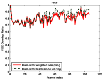
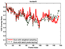
6) Evaluation of weighted reservoir sampling and batch mode learning. To balance effectiveness and efficiency, weighted reservoir sampling aims to maintain limited-sized foreground and background sample buffers used for learning a metric-weighted linear representation. In contrast, batch mode learning requires storing all the foreground and background samples during tracking, which leads to expensive computation and high memory usage. Therefore, we conduct a quantitative comparison experiment between weighted reservoir sampling and batch mode learning on three video sequences, as shown in Fig. 4. From Fig. 4, we observe that the tracking performance with weighted reservoir sampling is able to well approximate that of batch mode learning.
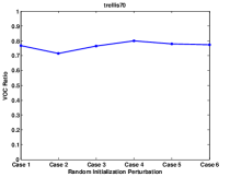
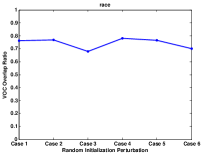
7) Effect of random initialization perturbation. Here, we aim to investigate the tracking performance of the proposed tracker with different initialization configurations, which are generated by moderate random perturbation (i.e., relatively small center location offset) on the original bounding box after manual initialization. Fig. 5 shows the average VOR tracking performance on three video sequences in different initialization cases. It is clearly seen from Fig. 5 that the proposed tracker achieves the mutually close tracking results, and is not sensitive to different initialization settings.
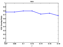
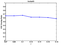
8) Investigation of the trade-off control factor . To evaluate the effect of the discriminative metric-weighted reconstruction information from foreground and background buffers, we make a quantitative empirical study of the proposed tracker with different configurations of (referred to in Equ. (3)). Fig. 6 displays the quantitative average VOR tracking results on three video sequences using different configurations of such that . Apparently, the proposed tracker is not very sensitive to the configuration of within a moderate range.
| CLE | VOR | Success Rate | ||||||||||||||||
|---|---|---|---|---|---|---|---|---|---|---|---|---|---|---|---|---|---|---|
| trellis70 | race | cubicle | football3 | trace | seq-jd | trellis70 | race | cubicle | football3 | trace | seq-jd | trellis70 | race | cubicle | football3 | trace | seq-jd | |
| ML w/o eigen | 5.62 | 8.52 | 4.31 | 3.92 | 8.65 | 4.30 | 0.78 | 0.80 | 0.74 | 0.69 | 0.70 | 0.72 | 0.98 | 0.99 | 0.98 | 0.97 | 0.89 | 0.94 |
| ML with final eigen | 8.46 | 10.17 | 5.95 | 7.80 | 18.38 | 7.06 | 0.70 | 0.69 | 0.67 | 0.54 | 0.52 | 0.63 | 0.94 | 0.99 | 0.94 | 0.55 | 0.57 | 0.82 |
| ML with step-by-step eigen | 4.56 | 6.23 | 2.16 | 3.84 | 7.46 | 3.12 | 0.83 | 0.75 | 0.78 | 0.74 | 0.75 | 0.76 | 0.99 | 0.99 | 0.98 | 0.98 | 0.98 | 0.97 |
| No metric learning | 8.82 | 16.80 | 5.29 | 5.07 | 16.94 | 6.09 | 0.68 | 0.65 | 0.67 | 0.63 | 0.51 | 0.64 | 0.92 | 0.97 | 0.88 | 0.91 | 0.40 | 0.85 |
IV-C Comparison with the state-of-the-art trackers
To demonstrate the effectiveness of the proposed tracking algorithm, we make a qualitative and quantitative comparison with several state-of-the-art trackers, referred to as FragT (Fragment-based tracker [50]), MILT (multiple instance boosting-based tracker [16]), VTD (visual tracking decomposition [4]), OAB (online AdaBoost [15]), IPCA (incremental PCA [3]), L1T ( minimization tracker [6]), CT (compressive tracker [10]), Struck (structured learning tracker [13]), DML (discriminative metric learning tracker [19]), TLD (tracking-learning-detection [51]), ASLA (adaptive structural local sparse model [52]), and SCM (sparsity-based collaborative model [53]). Moreover, the proposed tracking algorithm has two versions that are unstructured and structured (respectively referred to as Ours and Ours+S).


In the experiments, the following trackers are implemented using their publicly available source code: FragT, MILT, VTD, OAB, CT, Struck IPCA, L1T, TLD, ASLA, and SCM. For OAB, there are two different versions (namely, OAB1 and OAB5), which are based on two different configurations (i.e., the search scale and as in [16]).
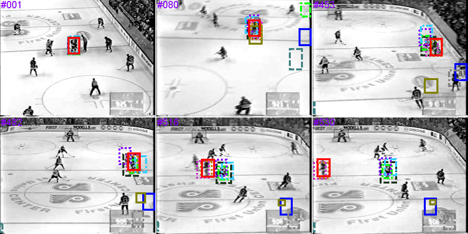
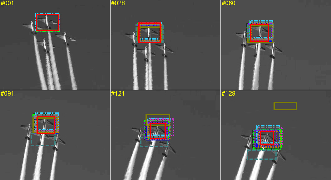
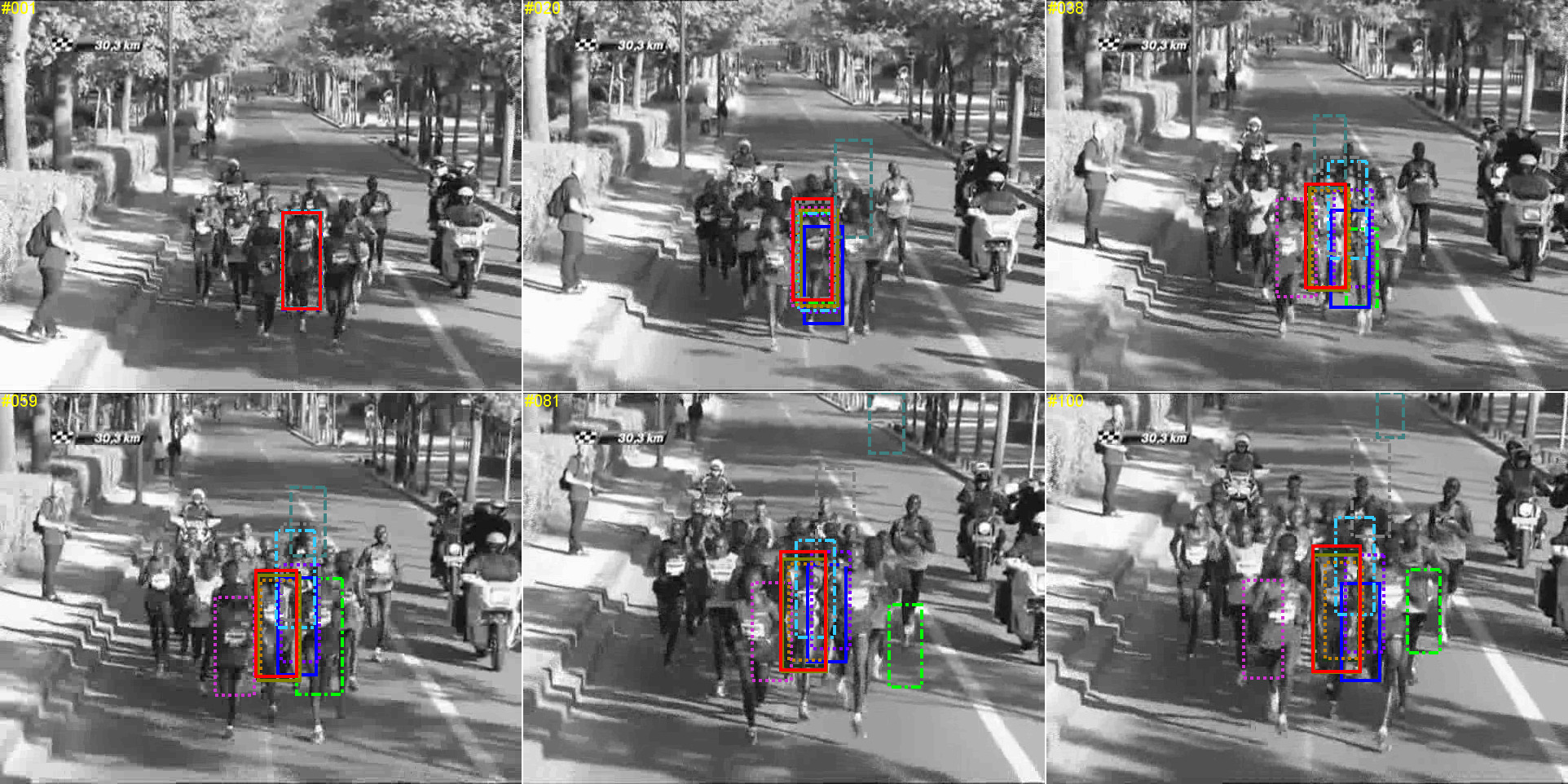
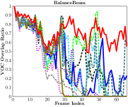
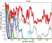
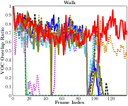
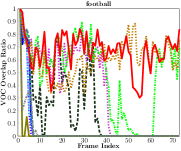
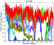
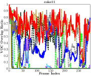
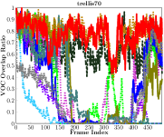
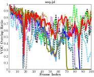
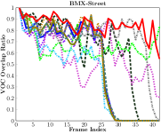
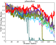
Figs. 35-41 show the qualitative tracking results of the eleven trackers on several sample frames on six video sequences. Fig. 33 and Tab. IV report the quantitative tracking results of the eleven trackers (in CLE, VOR, and success rate) over several video sequences. The complete tracking results and quantitative comparisons for all the eighteen video sequences can be found in the supplementary file. From Fig. 33 and Tab. IV, we observe that the proposed tracking algorithm achieves the best tracking performance by all measures on most video sequences. In the experiments, the TLD tracker (using the default parameter settings) produces the incomplete tracking results over some video sequences because of its particular tracking-learning-detection properties (i.e., tracking reliability analysis by simultaneously performing object detection and optical flow-based verification). Therefore, we only show the video sequences in which the TLD tracker can always achieve stable tracking performances for all the frames. The reasons for the incomplete tracking results are briefly analyzed as follows. In principle, the TLD tracker takes a tracking-by-detection strategy that needs to simultaneously perform object detection as well as optical flow-based tracking verification across successive frames. In the case of severe occlusions (or drastic pose changes or tiny objects or strong background clutters), it adaptively evaluates the tracking reliability by performing optical flow-based tracking verification or object classification (whose classification score may be very low), and is likely to remove the unreliable tracking results, leading to the tracking unavailability over several frames. With the emergence of the visually feasible tracked objects, the detection component of the TLD tracker is automatically activated to localize the tracked objects.
Subsequently, we briefly analyze the reasons why our tracker works well in some challenging situations. In essence, the foreground samples stored in the buffer approximately constitute an object manifold that contains the intrinsic structural information on object appearance. After distance metric learning, the object manifold encodes more discriminative information on object/non-object classification. If test samples are contaminated by some complicated factors (e.g., shape deformation, noisy corruption, and illumination variation), the intrinsic manifold structural properties of object appearance are very helpful to recover these test samples from contamination by manifold embedding (i.e., metric-weighted linear regression). Moreover, time-weighted reservoir sampling is able to ensure that the sample buffer retains useful old samples with a long lifespan and meanwhile adapts to recent appearance changes. Therefore, metric-weighted linear regression on such a sample buffer can not only alleviate the tracker drift problem but also adapt to complicated appearance changes. Besides, metric-weighted linear regression on the background buffer can generate the discriminative information to help the tracker reject several false foreground samples (caused by occlusion, out-of-plane rotation, and pose variation). Finally, the used features during tracking are extracted in a block-division manner. Therefore, they are capable of encoding the local geometrical information on object appearance, leading to the robustness to complicated scenarios (e.g., partial occlusion). Of course, when the appearance distinction between the foreground and background samples (especially for background clutter) is small, discriminative distance metric learning cannot improve the performance of metric-weighted linear regression. In this case, our tracker is incapable of accurately capturing the target location (e.g., the “coke11” sequence shown in Tab. IV) or even failing to track.
| B-Beam | Lola | trace | Walk | football | iceball | coke11 | trellis70 | dograce | football3 | cubicle | seq-jd | girl | B-Street | planeshow | race | CamSeq01 | car11 | ||
|---|---|---|---|---|---|---|---|---|---|---|---|---|---|---|---|---|---|---|---|
| CLE | Ours+S | 3.52 | 10.67 | 6.23 | 5.91 | 2.88 | 2.75 | 5.13 | 4.22 | 3.12 | 5.63 | 3.10 | 3.02 | 7.35 | 3.11 | 2.89 | 6.96 | 2.87 | 2.62 |
| Ours | 4.68 | 11.08 | 8.65 | 6.08 | 3.14 | 3.03 | 5.76 | 5.62 | 3.54 | 3.92 | 4.31 | 4.30 | 7.72 | 3.31 | 3.00 | 8.52 | 3.00 | 2.74 | |
| DML | 22.03 | 102.62 | 91.42 | 30.23 | 65.34 | 15.94 | 30.83 | 9.10 | 10.57 | 89.66 | 5.02 | 5.47 | 20.26 | 22.10 | 3.28 | 7.29 | 3.74 | 3.79 | |
| FragT | 46.61 | 141.00 | 19.70 | 92.46 | 31.95 | 13.86 | 59.54 | 39.86 | 8.43 | 28.52 | 25.54 | 5.83 | 20.92 | 15.29 | 10.04 | 45.28 | 9.20 | 65.31 | |
| VTD | 15.82 | 142.69 | 110.25 | 103.31 | 9.81 | 14.35 | 45.66 | 51.68 | 24.56 | 32.88 | 46.11 | 4.88 | 10.97 | 7.27 | 3.64 | 65.38 | 7.09 | 32.18 | |
| MILT | 19.08 | 138.97 | 68.00 | 37.08 | 103.59 | 76.09 | 17.71 | 60.41 | 7.97 | 9.23 | 43.53 | 16.24 | 39.96 | 41.16 | 4.99 | 25.55 | 13.26 | 44.79 | |
| OAB1 | 31.10 | 146.08 | 65.14 | 36.47 | 76.53 | 24.64 | 57.90 | 68.58 | 8.51 | 6.78 | 41.66 | 20.42 | 51.51 | 43.32 | 4.18 | 33.44 | 8.21 | 24.73 | |
| OAB5 | 24.15 | 67.16 | 66.31 | 36.74 | 97.16 | 37.00 | 64.97 | 126.36 | 18.56 | 14.87 | 37.06 | 11.71 | 67.13 | 47.71 | 11.30 | 42.18 | 5.85 | 9.85 | |
| IPCA | 41.64 | 127.88 | 80.60 | 37.33 | 133.67 | 41.60 | 56.60 | 46.13 | 6.70 | 31.99 | 33.61 | 24.16 | 20.90 | 41.69 | 28.02 | 5.26 | 21.22 | 2.42 | |
| L1T | 22.60 | 139.89 | 108.64 | 124.09 | 103.08 | 119.69 | 64.70 | 27.64 | 5.28 | 64.07 | 24.26 | 12.76 | 44.12 | 46.98 | 32.27 | 160.79 | 37.40 | 25.46 | |
| Struck | 28.62 | 139.90 | 24.15 | 10.83 | 3.24 | 3.76 | 5.50 | 4.82 | 4.54 | 4.32 | 22.61 | 3.32 | 7.38 | 42.06 | 5.77 | 7.71 | 6.54 | 2.09 | |
| CT | 37.22 | 23.04 | 41.59 | 35.94 | 106.72 | 29.97 | 15.83 | 50.97 | 8.98 | 13.50 | 45.78 | 22.06 | 34.10 | 9.33 | 6.61 | 76.20 | 11.34 | 29.43 | |
| ALSA | 15.73 | 30.50 | 23.11 | 28.14 | 3.99 | 3.17 | 12.98 | 4.99 | 11.20 | 31.23 | 25.34 | 20.19 | 36.87 | 6.44 | 3.19 | 35.41 | 10.38 | 2.05 | |
| SCM | 16.98 | 22.94 | 20.35 | 31.81 | 26.60 | 3.56 | 94.74 | 12.30 | 8.68 | 36.85 | 23.04 | 11.66 | 7.47 | 8.25 | 5.18 | 33.12 | 7.17 | 1.92 | |
| TLD | - | - | - | - | - | - | 9.73 | 13.11 | - | - | 19.58 | - | 19.15 | - | - | - | 9.10 | - | |
| VOR | Ours+S | 0.78 | 0.67 | 0.74 | 0.73 | 0.69 | 0.71 | 0.65 | 0.83 | 0.67 | 0.72 | 0.78 | 0.76 | 0.78 | 0.86 | 0.80 | 0.82 | 0.83 | 0.77 |
| Ours | 0.72 | 0.66 | 0.70 | 0.72 | 0.67 | 0.69 | 0.65 | 0.78 | 0.66 | 0.72 | 0.74 | 0.72 | 0.78 | 0.85 | 0.79 | 0.80 | 0.82 | 0.76 | |
| DML | 0.43 | 0.18 | 0.20 | 0.54 | 0.21 | 0.47 | 0.36 | 0.65 | 0.54 | 0.36 | 0.68 | 0.68 | 0.60 | 0.63 | 0.68 | 0.78 | 0.79 | 0.69 | |
| FragT | 0.24 | 0.13 | 0.51 | 0.09 | 0.36 | 0.44 | 0.05 | 0.34 | 0.54 | 0.30 | 0.35 | 0.67 | 0.64 | 0.57 | 0.64 | 0.23 | 0.65 | 0.08 | |
| VTD | 0.49 | 0.06 | 0.12 | 0.09 | 0.50 | 0.52 | 0.11 | 0.33 | 0.38 | 0.32 | 0.20 | 0.70 | 0.73 | 0.67 | 0.66 | 0.16 | 0.74 | 0.37 | |
| MILT | 0.41 | 0.03 | 0.34 | 0.50 | 0.06 | 0.13 | 0.35 | 0.29 | 0.59 | 0.55 | 0.18 | 0.53 | 0.39 | 0.50 | 0.71 | 0.34 | 0.63 | 0.15 | |
| OAB1 | 0.34 | 0.04 | 0.35 | 0.46 | 0.05 | 0.26 | 0.04 | 0.16 | 0.57 | 0.63 | 0.21 | 0.47 | 0.34 | 0.47 | 0.73 | 0.28 | 0.64 | 0.37 | |
| OAB5 | 0.40 | 0.13 | 0.36 | 0.45 | 0.05 | 0.21 | 0.04 | 0.06 | 0.35 | 0.40 | 0.24 | 0.46 | 0.24 | 0.39 | 0.58 | 0.36 | 0.74 | 0.43 | |
| IPCA | 0.30 | 0.05 | 0.26 | 0.46 | 0.02 | 0.19 | 0.03 | 0.36 | 0.65 | 0.23 | 0.30 | 0.45 | 0.62 | 0.50 | 0.51 | 0.79 | 0.49 | 0.78 | |
| L1T | 0.41 | 0.07 | 0.09 | 0.09 | 0.06 | 0.07 | 0.03 | 0.28 | 0.67 | 0.16 | 0.41 | 0.52 | 0.46 | 0.50 | 0.33 | 0.08 | 0.27 | 0.43 | |
| Struck | 0.35 | 0.11 | 0.43 | 0.65 | 0.60 | 0.68 | 0.66 | 0.80 | 0.64 | 0.72 | 0.41 | 0.76 | 0.78 | 0.52 | 0.73 | 0.66 | 0.68 | 0.79 | |
| CT | 0.25 | 0.30 | 0.33 | 0.45 | 0.03 | 0.47 | 0.41 | 0.22 | 0.57 | 0.43 | 0.17 | 0.45 | 0.45 | 0.75 | 0.69 | 0.26 | 0.63 | 0.29 | |
| ALSA | 0.47 | 0.39 | 0.40 | 0.51 | 0.57 | 0.60 | 0.42 | 0.78 | 0.55 | 0.30 | 0.24 | 0.46 | 0.39 | 0.76 | 0.60 | 0.18 | 0.66 | 0.79 | |
| SCM | 0.36 | 0.42 | 0.43 | 0.50 | 0.27 | 0.61 | 0.11 | 0.70 | 0.57 | 0.29 | 0.45 | 0.48 | 0.76 | 0.71 | 0.65 | 0.23 | 0.71 | 0.77 | |
| TLD | - | - | - | - | - | - | 0.56 | 0.69 | - | - | 0.48 | - | 0.66 | - | - | - | 0.70 | - | |
| Success Rate | Ours+S | 0.95 | 0.81 | 0.98 | 0.99 | 0.90 | 0.94 | 0.88 | 0.99 | 0.98 | 0.97 | 0.98 | 0.96 | 0.99 | 0.98 | 0.99 | 0.99 | 0.99 | 1.00 |
| Ours | 0.94 | 0.80 | 0.89 | 0.98 | 0.88 | 0.93 | 0.87 | 0.98 | 0.97 | 0.97 | 0.98 | 0.95 | 0.99 | 0.97 | 0.98 | 0.99 | 0.99 | 1.00 | |
| DML | 0.43 | 0.18 | 0.12 | 0.67 | 0.20 | 0.59 | 0.37 | 0.90 | 0.60 | 0.46 | 0.82 | 0.85 | 0.79 | 0.74 | 0.86 | 0.99 | 0.99 | 0.92 | |
| FragT | 0.25 | 0.11 | 0.63 | 0.09 | 0.47 | 0.52 | 0.05 | 0.40 | 0.49 | 0.32 | 0.37 | 0.88 | 0.79 | 0.51 | 0.71 | 0.22 | 0.90 | 0.08 | |
| VTD | 0.57 | 0.07 | 0.11 | 0.11 | 0.62 | 0.70 | 0.10 | 0.37 | 0.47 | 0.31 | 0.20 | 0.79 | 0.92 | 0.98 | 0.78 | 0.20 | 0.99 | 0.43 | |
| MILT | 0.37 | 0.03 | 0.42 | 0.64 | 0.07 | 0.16 | 0.28 | 0.34 | 0.67 | 0.61 | 0.22 | 0.61 | 0.19 | 0.58 | 0.89 | 0.18 | 0.87 | 0.08 | |
| OAB1 | 0.37 | 0.01 | 0.40 | 0.62 | 0.05 | 0.14 | 0.04 | 0.13 | 0.67 | 0.87 | 0.22 | 0.58 | 0.18 | 0.58 | 0.88 | 0.19 | 0.80 | 0.39 | |
| OAB5 | 0.43 | 0.08 | 0.42 | 0.67 | 0.05 | 0.12 | 0.04 | 0.03 | 0.23 | 0.24 | 0.22 | 0.38 | 0.14 | 0.53 | 0.69 | 0.25 | 0.91 | 0.33 | |
| IPCA | 0.34 | 0.06 | 0.31 | 0.62 | 0.01 | 0.09 | 0.03 | 0.38 | 0.87 | 0.22 | 0.25 | 0.45 | 0.80 | 0.58 | 0.74 | 0.99 | 0.60 | 1.00 | |
| L1T | 0.43 | 0.07 | 0.06 | 0.11 | 0.07 | 0.08 | 0.04 | 0.34 | 0.87 | 0.16 | 0.49 | 0.61 | 0.57 | 0.58 | 0.45 | 0.10 | 0.28 | 0.59 | |
| Struck | 0.40 | 0.13 | 0.37 | 0.83 | 0.74 | 0.95 | 0.93 | 0.96 | 0.83 | 0.96 | 0.47 | 0.97 | 0.99 | 0.58 | 0.89 | 0.88 | 0.93 | 1.00 | |
| CT | 0.27 | 0.15 | 0.29 | 0.64 | 0.01 | 0.67 | 0.35 | 0.12 | 0.60 | 0.27 | 0.22 | 0.47 | 0.37 | 0.88 | 0.83 | 0.20 | 0.89 | 0.17 | |
| ALSA | 0.46 | 0.31 | 0.41 | 0.68 | 0.65 | 0.73 | 0.40 | 0.95 | 0.58 | 0.31 | 0.20 | 0.48 | 0.37 | 0.93 | 0.70 | 0.20 | 0.96 | 1.00 | |
| SCM | 0.30 | 0.53 | 0.42 | 0.66 | 0.32 | 0.78 | 0.12 | 0.84 | 0.61 | 0.30 | 0.63 | 0.49 | 0.99 | 0.91 | 0.83 | 0.23 | 0.94 | 1.00 | |
| TLD | - | - | - | - | - | - | 0.70 | 0.81 | - | - | 0.63 | - | 0.90 | - | - | - | 0.96 | - |
Moreover, time weighted reservoir sampling can alleviate error accumulation during tracking. Although some false foreground/background samples may be added to the buffers because of tracking errors, the old samples with a long lifespan can effectively reduce the influence of the false foreground/background samples on metric-weighted least square regression, leading to robust tracking results. In other words, the metric-weighted least square regression problem has two types of reconstruction costs. One is based on the old samples with a long lifespan, and the other relies on the recent samples. Actually, the regression cost for the old samples with a long lifespan works as a regularizer that can resist tracker drift. In addition, metric-weighted linear regression on the background buffer can generate the discriminative information to help the tracker reject false foreground samples (caused by occlusion, out-of-plane rotation, and pose variation). For instance, some false foreground training samples are included into the foreground sample buffer at the 18th frame of the “seq-jd” video sequence because of partial occlusions, as shown in the supplementary demo video files. After the 19th frame (without occlusions), our tracker is still able to accurately localize the head target with the help of discriminative metric-weighted linear regression on the foreground and background sample suffers.


Fig. 14 shows a failure case for our method during the “coke11” video sequence. As shown in Fig. 14(a), the appearance difference between the tracked object and its surrounding background is relatively small (i.e., they appear to be visually edgeless or textureless). As a result, the foreground and background metric-weighted linear reconstruction costs for these regions with respect to a set of foreground or background basis samples are mutually close, resulting in a low confidence score for discriminative object/non-object classification with several false detection hypotheses. Based on structured SVM learning for optimizing the structural localization measure, Struck is capable of encoding the joint feature-location contextual information on object appearance, leading to a relatively stable tracking result. As shown in Fig. 14(b), a severe occlusion event leads to the almost complete disappearance of the tracked object. Consequently, both of the trackers fail to track in this scenario.
Potentially, the further performance improvement can be made in the following two respects: 1) the current versions of the trackers are still based on several hand-crafted visual features (e.g., HOG and Haar), which are weak in adaptively capturing the intrinsic discriminative appearance properties of the tracked objects in various scenarios. Therefore, adaptive online feature learning is a potential solution to this issue. 2) the integration of tracking reliability analysis could handle some abnormal events like severe occlusions. If and only if the tracking results are very reliable, then the detectors or classifiers can be updated.
The most competitive method to ours is Struck [13], which achieves a comparable or better tracking performance on five of the eighteen sequences. Struck is based on structured learning, and directly optimizes the VOC overlap criterion using a structured SVM formulation. In the following section, we extend our framework to optimize this same criterion and re-evaluate against Struck.
IV-D Empirical evaluation of structured metric learning
| CLE | VOR | Success Rate | ||||||||||||||||
|---|---|---|---|---|---|---|---|---|---|---|---|---|---|---|---|---|---|---|
| trellis70 | race | cubicle | football3 | trace | seq-jd | trellis70 | race | cubicle | football3 | trace | seq-jd | trellis70 | race | cubicle | football3 | trace | seq-jd | |
| Struck | 4.82 | 7.71 | 22.61 | 4.32 | 24.15 | 3.32 | 0.80 | 0.66 | 0.41 | 0.72 | 0.43 | 0.76 | 0.96 | 0.88 | 0.47 | 0.96 | 0.37 | 0.97 |
| Non-structured metric learning | 5.62 | 8.52 | 4.31 | 3.92 | 8.65 | 4.30 | 0.78 | 0.80 | 0.74 | 0.72 | 0.70 | 0.72 | 0.98 | 0.99 | 0.98 | 0.97 | 0.89 | 0.95 |
| Structured metric learning | 4.22 | 6.96 | 3.10 | 5.63 | 6.23 | 3.02 | 0.83 | 0.82 | 0.78 | 0.72 | 0.74 | 0.76 | 0.99 | 0.99 | 0.98 | 0.97 | 0.98 | 0.96 |
| No metric learning | 7.80 | 15.86 | 4.43 | 4.01 | 15.75 | 5.16 | 0.73 | 0.69 | 0.70 | 0.68 | 0.56 | 0.68 | 0.93 | 0.99 | 0.96 | 0.95 | 0.62 | 0.94 |
To evaluate the effect of structured metric learning, we compare its tracking performance to our previous method on eight video sequences. For computational efficiency, the structured metric learning method takes a uniform sampling strategy to randomly generate a collection of bounding boxes around the current tracker bounding box. Using these bounding boxes, we construct a set of triplet-based structural constraints (referred to in Equ. (14)) for online structured metric learning.
Tab. V reports their average frame-by-frame VORs, CLEs, and success rates on the four video sequences. Clearly, it is seen from Tab. V that the structured metric learning method outperforms both the non-structured metric learning method and the method without metric learning.
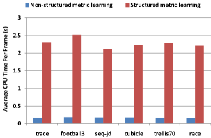
In addition, Fig. 15 shows the average runtime performance of the tracking approach using non-structured or structured metric learning on the eight video sequences. It is clearly seen from Fig. 15 that structured metric learning is about 20 times slower than non-structured metric learning. From Tab. V, we see that non-structured metric learning achieves a reasonably close tracking performance to structured metric learning. However, the computational efficiency of non-structured metric learning is much better than that of structured metric learning. Therefore, in the applications presented in the next Section, we use non-structured metric learning.
The Struck tracker constructs an object localization scoring function based on structured SVM learning, which learns a linear SVM scoring function in a max-margin structured output optimization framework. Therefore, the tracking accuracy of the Struck tracker solely depends on the learned SVM scoring function. In the case of tracking errors, the learned SVM scoring function is contaminated, causing the error accumulations across frames, which often leads to tracker drift in complicated scenarios. In contrast, our tracker takes a data-driven strategy for object localization. Namely, our tracker takes advantage of reservoir sampling to effectively maintain the foreground/background buffers, which store the recently included samples while keeping the old samples with a long lifespan. Besides, our metric-weighted linear regression cost based on these old samples essentially works as a regularizer that reduces the influence of the tracking error accumulations, resulting in the tracking robustness. Combined with structured metric learning, our tracker has the capability of performing robust visual tracking in a more discriminative metric space, leading to the further performance improvements.
IV-E Experimental summary
Based on the obtained experimental results, we observe that the proposed tracking algorithm has the following properties. First, after the buffer size exceeds a certain value (around in our experiments), the tracking performance is stable with increasing buffer size, as shown in Fig. 3. This is desirable since we do not need a large buffer size to achieve promising performance. Second, in contrast to many existing particle filtering-based trackers whose running time is typically linear in the number of particles, our method’s running time is sublinear in the number of particles, as shown in Fig. 3. Moreover, its tracking performance rapidly improves and finally converge to a certain value, as shown in Fig. 3. Third, based on linear representation with metric learning, it performs better in tracking accuracy, as shown in Tab. I. Fourth, it utilizes weighted reservoir sampling to effectively maintain and update the foreground and background sample buffers for metric learning, as shown in Tab. II. Fifth, as shown in Tab. VII, the performance of our metric learning with no eigendecomposition is close to that of computationally expensive metric learning with step-by-step eigendecomposition. Sixth, compared with other state-of-the-art trackers, it is capable of effectively adapting to complicated appearance changes in the tracking process by constructing an effective metric-weighted linear representation with weighed reservoir sampling, as shown in Tab. IV. Last, using the structured metric learning is capable of improving the tracking performance in CLE and VOR, as shown in Tab. V. That is because the structured metric learning encodes the underlying the structural interaction information on data samples, which plays an important role in robust visual tracking.
V Pedestrian tracking and identification
Recent studies have demonstrated the effectiveness of combining object identification and tracking together. To achieve this goal, we need to first localize the object of interest and then assign it to one of the predefined object classes using the object tracking information. Without loss of generality, we suppose there are totally object classes that correspond to static template sample sets (collected before object tracking). After performing object tracking on a video sequence ranging from frame 1 to frame , we obtain the consecutive object observations whose object classification scores are denoted as (as defined in Equ. (3)). In essence, these classification scores reflect the likelihood of the observations to be generated from the object of interest. With respect to , we compute a set of reconstruction errors such that . Based on these reconstruction errors, the cumulative distance of with respect to the -th object class is calculated as:
| (19) |
where is a weighting factor that measures the prior weight of generated from the object of interest. Here, we just use the object classification score to approximate the prior weight in the process of object identification (such that ). As a result, the object class membership for is determined by: . In addition, the above-mentioned object identification module has the capability of automatically detecting the abnormal events (e.g., occlusion). When is very large, the tracked objects often have drastic appearance changes (caused by occlusion, noisy corruption, shape deformation, and so on). Therefore, the abnormal changes in object appearance can be automatically detected by checking the value of .
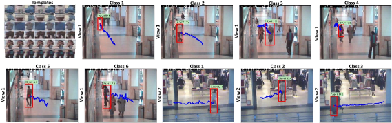

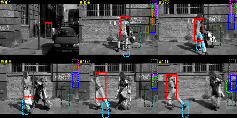
Based on Equ. (19), we carry out the pedestrian identification task on the video sequences111http://homepages.inf.ed.ac.uk/rbf/CAVIARDATA1/ with two viewpoints. Prior to pedestrian tracking and identification, we collect a set of static templates from some training video sequences. In total, there are six individual pedestrians corresponding to six object classes. Fig. 16 shows the pedestrian tracking and identification results as well as the static templates used in tracking. For a clear illustration, we give an intuitive example of showing the whole pedestrian identification process, as shown in Fig. 17. From Fig. 17, we observe that our method is able to accurately recognize the tracked pedestrian’s identity throughout the entire video sequence. More pedestrian identification results can be found in the supplementary.

Moreover, we apply our method to detect whether the abnormal events (e.g., occlusion) take place in the tracking process. Namely, if the target appearance is weakly correlated with the static templates (i.e., high reconstruction errors), there is likely to be some abnormal events occurring during tracking. Fig. 18 shows an example of detecting the frame-by-frame occlusion events on the “girl” video sequence. It is seen from Fig. 18 that our method succeeds in detecting the occlusion events in most cases.
VI Conclusion
In this work, we have proposed an online metric-weighted linear representation for robust visual tracking. With a closed-form analytical solution, the proposed linear representation is capable of effectively encoding the discriminative information on object/non-object classification. We designed an online Mahalanobis distance metric learning scheme, including online non-structured and structured metric learning. The metric learning scheme aims to distinguish the relative importance of individual feature dimensions and capture the correlation between feature dimensions in a feasible metric space. We empirically show that adding a metric to the linear representation considerably improves the robustness of the tracker. To make the online metric learning even more efficient, for the first time, we design a learning mechanism based on time-weighted reservoir sampling. With this mechanism, recently streamed samples in the video are assigned higher weights. We have also theoretically proved that metric learning based on the proposed reservoir sampling with limited-sized sampling buffers can effectively approximate metric learning using all the received training samples. Compared with state-of-the-art trackers on eighteen challenging sequences, we empirically show that our method is more robust to complicated appearance changes, pose variations, and occlusions. Furthermore, we also extend our work to perform pedestrian identification and occlusion event detection during object tracking. Experimental results demonstrate the effectiveness of our work.
To balance efficiency and effectiveness, a mixture of non-structured and structured metric learning methods can be alternatively applied during tracking. For example, the non-structured method can produce metric learning results with a high update frequency, and then the structured method further generates the refined metric learning results with a low update frequency. We plan to investigate this in future.
References
- [1] D. W. Park, J. Kwon, and K. M. Lee, “Robust visual tracking using autoregressive hidden markov model,” in Proc. IEEE Conf. Comp. Vis. Patt. Recogn., 2012, pp. 1964–1971.
- [2] A. D. Jepson, D. J. Fleet, and T. F. El-Maraghi, “Robust online appearance models for visual tracking,” in Proc. IEEE Conf. Comp. Vis. Patt. Recogn., 2001, pp. 415–422.
- [3] D. A. Ross, J. Lim, R. Lin, and M. Yang, “Incremental learning for robust visual tracking,” Int. J. Comp. Vis., vol. 77, no. 1, pp. 125–141, 2008.
- [4] J. Kwon and K. M. Lee, “Visual tracking decomposition,” in Proc. IEEE Conf. Comp. Vis. Patt. Recogn., 2010, pp. 1269–1276.
- [5] T. Zhang, G. B, S. Liu, and N. Ahuja, “Robust visual tracking via structured multi-task sparse learning,” Int. J. Comp. Vis., vol. 101, no. 2, pp. 367–383, 2013.
- [6] X. Mei and H. Ling, “Robust visual tracking and vehicle classification via sparse representation,” IEEE Trans. Pattern Anal. Mach. Intell., 2011.
- [7] H. Li, C. Shen, and Q. Shi, “Real-time visual tracking with compressive sensing,” in Proc. IEEE Conf. Comp. Vis. Patt. Recogn., 2011.
- [8] D. Wang, H. Lu, and M. Yang, “Online object tracking with sparse prototypes,” IEEE Trans. Image Proc., vol. 22, no. 1, pp. 314–325, 2013.
- [9] Y. Wu, J. Cheng, J. Wang, H. Lu, J. Wang, H. Ling, E. Blasch, and L. Bai, “Real-time probabilistic covariance tracking with efficient model update,” IEEE Trans. Image Proc., vol. 21, no. 5, pp. 2824–2837, 2012.
- [10] K. Zhang, L. Zhang, and M. Yang, “Real-time compressive tracking,” in Proc. Eur. Conf. Comp. Vis., 2012, pp. 864–877.
- [11] S. Avidan, “Support vector tracking,” IEEE Trans. Pattern Anal. Mach. Intell., vol. 26, no. 8, pp. 1064–1072, 2004.
- [12] Y. Bai and M. Tang, “Robust tracking via weakly supervised ranking svm,” in Proc. IEEE Conf. Comp. Vis. Patt. Recogn., 2012, pp. 1854–1861.
- [13] S. Hare, A. Saffari, and P. Torr, “Struck: Structured output tracking with kernels,” in Proc. IEEE Int. Conf. Comp. Vis., 2011.
- [14] B. Khanloo, F. Stefanus, M. Ranjbar, Z. Li, N. Saunier, T. Sayed, and G. Mori, “A large margin framework for single camera offline tracking with hybrid cues,” Computer Vision and Image Understanding, vol. 116, no. 6, pp. 676–689, 2012.
- [15] H. Grabner, M. Grabner, and H. Bischof, “Real-time tracking via on-line boosting,” in Proc. British Machine Vis. Conf., 2006, pp. 47–56.
- [16] B. Babenko, M. Yang, and S. Belongie, “Visual tracking with online multiple instance learning,” in Proc. IEEE Conf. Comp. Vis. Patt. Recogn., 2009, pp. 983–990.
- [17] J. Santner, C. Leistner, A. Saffari, T. Pock, and H. Bischof, “Prost: Parallel robust online simple tracking,” in Proc. IEEE Conf. Comp. Vis. Patt. Recogn., 2010, pp. 723–730.
- [18] J. Fan, Y. Wu, and S. Dai, “Discriminative spatial attention for robust tracking,” in Proc. Eur. Conf. Comp. Vis., 2010, pp. 480–493.
- [19] X. Wang, G. Hua, and T. Han, “Discriminative tracking by metric learning,” Proc. Eur. Conf. Comp. Vis., pp. 200–214, 2010.
- [20] G. Tsagkatakis and A. Savakis, “Online distance metric learning for object tracking,” IEEE Trans. Circuits & Systems for Video Tech., 2011.
- [21] Z. Kalal, K. Mikolajczyk, and J. Matas, “Tracking-learning-detection,” IEEE Trans. Pattern Anal. Mach. Intell., vol. 34, no. 7, pp. 1409–1422, 2012.
- [22] G. Chechik, V. Sharma, U. Shalit, and S. Bengio, “Large scale online learning of image similarity through ranking,” J. Mach. Learn. Research, vol. 11, pp. 1109–1135, 2010.
- [23] C. Bao, Y. Wu, H. Ling, and H. Ji, “Real time robust l1 tracker using accelerated proximal gradient approach,” in Proc. IEEE Conf. Comp. Vis. Patt. Recogn., 2012, pp. 1830–1837.
- [24] R. Rigamonti, M. A. Brown, and V. Lepetit, “Are sparse representations really relevant for image classification?” in Proc. IEEE Conf. Comp. Vis. Patt. Recogn., 2011, pp. 1545–1552.
- [25] L. Zhang, M. Yang, and X. Feng, “Sparse representation or collaborative representation: Which helps face recognition?” in Proc. IEEE Int. Conf. Comp. Vis., 2011.
- [26] X. Li, A. Dick, C. Shen, A. van den Hengel, and H. Wang, “Incremental learning of 3d-dct compact representations for robust visual tracking,” IEEE Trans. Pattern Anal. Mach. Intell., vol. 35, no. 4, pp. 863–881, 2013.
- [27] K. Weinberger, J. Blitzer, and L. Saul, “Distance metric learning for large margin nearest neighbor classification,” in Proc. Adv. Neural Inf. Process. Syst., 2006.
- [28] T. Mensink, J. Verbeek, F. Perronnin, and G. Csurka, “Metric learning for large scale image classification: Generalizing to new classes at near-zero cost,” in Proc. Eur. Conf. Comp. Vis., 2012, pp. 488–501.
- [29] D. Kedem, S. Tyree, K. Weinberger, F. Sha, and G. Lanckriet, “Non-linear metric learning,” in Proc. Adv. Neural Inf. Process. Syst., 2012, pp. 2582–2590.
- [30] Y. Ying and P. Li, “Distance metric learning with eigenvalue optimization,” J. Mach. Learn. Res., vol. 13, pp. 1–26, 2012.
- [31] N. Jiang, W. Liu, and Y. Wu, “Adaptive and discriminative metric differential tracking,” in Proc. IEEE Conf. Comp. Vis. Patt. Recogn., 2011, pp. 1161–1168.
- [32] Z. Hong, X. Mei, and D. Tao, “Dual-force metric learning for robust distracter-resistant tracker,” in Proc. Eur. Conf. Comp. Vis., 2012, pp. 513–527.
- [33] J. S. Vitter, “Random sampling with a reservoir,” ACM Trans. Math. Software, vol. 11, no. 1, pp. 37–57, 1985.
- [34] P. Zhao, S. Hoi, R. Jin, and T. Yang, “Online AUC maximization,” in Proc. Int. Conf. Mach. Learn., 2011.
- [35] X. Jia, H. Lu, and M. Yang, “Visual tracking via adaptive structural local sparse appearance model,” in Proc. IEEE Conf. Comp. Vis. Patt. Recogn., 2012, pp. 1822–1829.
- [36] W. Zhong, H. Lu, and M. Yang, “Robust object tracking via sparsity-based collaborative model,” in Proc. IEEE Conf. Comp. Vis. Patt. Recogn., 2012, pp. 1838–1845.
- [37] X. Li, A. Dick, C. Shen, Z. Zhang, A. van den Hengel, and H. Wang, “Visual tracking with spatio-temporal dempster-shafer information fusion.” IEEE Trans. Image Proc., vol. 22, no. 8, pp. 3028–3040, 2013.
- [38] G. J. Edwards, C. J. Taylor, and T. F. Cootes, “Improving identification performance by integrating evidence from sequences,” in Proc. IEEE Conf. Comp. Vis. Patt. Recogn., 1999.
- [39] S. K. Zhou, R. Chellappa, and B. Moghaddam, “Visual tracking and recognition using appearance-adaptive models in particle filters,” IEEE Trans. Image Proc., vol. 13, no. 11, pp. 1491–1506, 2004.
- [40] X. Li, C. Shen, Q. Shi, A. Dick, and A. v. d. Hengel, “Non-sparse linear representations for visual tracking with online reservoir metric learning,” in Proc. IEEE Conf. Comp. Vis. Patt. Recogn., 2012, pp. 1760–1767.
- [41] M. Isard and A. Blake, “Contour tracking by stochastic propagation of conditional density,” in Proc. Eur. Conf. Comp. Vis., 1996, pp. 343–356.
- [42] A. Jennings and J. McKeown, Matrix computation. John Wiley & Sons Inc., 1992.
- [43] K. Crammer, O. Dekel, J. Keshet, S. Shalev-Shwartz, and Y. Singer, “Online passive-aggressive algorithms,” J. Mach. Learn. Research, vol. 7, pp. 551–585, 2006.
- [44] A. S. Householder, The theory of matrices in numerical analysis. Blaisdell Publishing Co.: New York, 1964.
- [45] M. J. D. Powell, “A theorem on rank one modifications to a matrix and its inverse,” The Computer Journal, vol. 12, no. 3, pp. 288–290, 1969.
- [46] M. Kolonko and D. Wäsch, “Sequential reservoir sampling with a non-uniform distribution,” ACM Trans. Math. Software, vol. 32, pp. 257–273, 2004.
- [47] P. S. Efraimidis and P. G. Spirakis, “Weighted random sampling with a reservoir,” Information process. letters, vol. 97, no. 5, pp. 181–185, 2006.
- [48] N. Dalal and B. Triggs, “Histograms of oriented gradients for human detection,” in Proc. IEEE Conf. Comp. Vis. Patt. Recogn., 2005.
- [49] X. Li, W. Hu, Z. Zhang, X. Zhang, M. Zhu, and J. Cheng, “Visual tracking via incremental log-euclidean riemannian subspace learning,” in Proc. IEEE Conf. Comp. Vis. Patt. Recogn., 2008, pp. 1–8.
- [50] A. Adam, E. Rivlin, and I. Shimshoni, “Robust fragments-based tracking using the integral histogram,” in Proc. IEEE Conf. Comp. Vis. Patt. Recogn., 2006, pp. 798–805.
- [51] Z. Kalal, K. Mikolajczyk, and J. Matas, “Tracking-learning-detection,” IEEE Trans. Pattern Anal. Mach. Intell., vol. 34, no. 7, pp. 1409–1422, 2012.
- [52] X. Jia, H. Lu, and M. Yang, “Visual tracking via adaptive structural local sparse appearance model,” in Proc. IEEE Conf. Comp. Vis. Patt. Recogn., 2012, pp. 1822–1829.
- [53] W. Zhong, H. Lu, and M. Yang, “Robust object tracking via sparsity-based collaborative model,” in Proc. IEEE Conf. Comp. Vis. Patt. Recogn., pp. 1838–1845.
Supplementary
In this supplementary material, we provide more technical details of online updating the metric-weighted linear representation, online discriminative distance metric learning, and a theoretical analysis of time-weighted reservoir sampling. Furthermore, we show more experimental results (both qualitatively and quantitatively), including experimental demonstration videos, more CLE (center location error) and VOR (VOC overlap ratio) curves for different evaluation tasks, intuitive frame tracking images, and more frame-by-frame pedestrian identification results.
| Video sequences | Corresponding video files |
|---|---|
| B-Beam | Video_01_BalanceBeam.mp4 |
| Lola | Video_02_Lola.mp4 |
| trace | Video_03_trace.mp4 |
| Walk | Video_04_Walk.mp4 |
| football | Video_05_football.mp4 |
| iceball | Video_06_iceball.mp4 |
| coke11 | Video_07_coke11.mp4 |
| trellis70 | Video_08_trellis70.mp4 |
| dograce | Video_09_dograce.mp4 |
| football3 | Video_10_football3.mp4 |
| cubicle | Video_11_cubicle.mp4 |
| seq-jd | Video_12_seq-jd.mp4 |
| girl | Video_13_girl.mp4 |
| BMX-Street | Video_14_BMX-Street.mp4 |
| planeshow | Video_15_planeshow.mp4 |
| race | Video_16_race.mp4 |
| CamSeq01 | Video_17_CamSeq01.mp4 |
| car11 | Video_18_car11.mp4 |
VII Online proximity based metric learning
Having introduced the metric-weighted linear representation in Sec. III-B, we now address the key issue of calculating the metric matrix . should ideally be learned from the visual data, and should be dynamically updated as conditions change throughout a video sequence.
VII-1 Triplet-based ranking losses
Suppose that we have a set of sample triplets with . These triplets encode the proximity comparison information. In each triplet, the distance between and should be smaller than the distance between and .
The Mahalanobis distance under metric is defined as:
| (20) |
Clearly, must be a symmetric and positive semidefinite matrix. It is equivalent to learn a projection matrix such that . In practice, we generate the triplets set as: and belong to the same class and and belong to different classes. So we want the constraints to be satisfied as well as possible. By putting it into a large-margin learning framework, and using the soft-margin hinge loss, the loss function for each triplet is:
| (21) |
VII-2 Large-margin metric learning
To obtain the optimal distance metric matrix , we need to minimize the global loss that takes the sum of hinge losses (21) over all possible triplets from the training set:
| (22) |
where is the triplet set. To sequentially optimize the above objective function in an online fashion, we design an iterative algorithm to solve the following convex problem:
| (23) |
where denotes the Frobenius norm, is a slack variable, and is a positive factor controlling the trade-off between the smoothness term and the loss term . Following the passive-aggressive mechanism used in [22, 43], we only update the metric matrix when .
VII-3 Optimization of
We optimize the function in Equation 23 with Lagrangian regularization:
| (24) |
where and are Lagrange multipliers. The optimization procedure is carried out in the following two alternating steps.
-
•
Update . By setting , we arrive at the update rule
(25) where and , .
By taking the derivative of w.r.t. , we have the following:
(26) Mathematically, can be formulated as:
(27) where and . The optimal is obtained by setting to zero. As a result, the following relation holds:
(28) -
•
Update . Subsequently, we take the derivative of the Lagrangian (24) w.r.t. and set it to zero, leading to the update rule:
(29) Clearly, leads to the fact that . For notational simplicity, is abbreviated as hereinafter. By substituting Equs. (28) and (29) into Equ. (24) with , we have:
(30) where and . As a result, can be reformulated as:
(31) where , , and . To obtain the optimal , we need to differentiate w.r.t. and set it to zero:
(32) As a result, the following relation holds:
(33) Due to the constraint of , should take the following value:
(34)
The full derivation of each step can be found in the supplementary file. The complete procedure of online distance metric learning is summarized in Algorithm 2.
VII-4 Online update
When updated according to Algorithm 2, is modified by rank-one additions such that where and are two vectors (defined in Equ. (28)) for triplet construction, and is a step-size factor (defined in Equ. (34)). As a result, the original becomes . When is modified by a rank-one addition, the inverse of can be updated according to the theory of [44, 45]:
| (35) |
Here, , (or ), and (or ).
VIII Online structured metric learning
Metric learning based on sample proximity comparisons leads to an efficient online learning algorithm, but requires pre-defined sets of positive and negative samples. In tracking, these usually correspond to target/non-target image patches. The boundary between these classes typically occurs where sample overlap with the target drops below a threshold, but this can be difficult to evaluate exactly and thus introduces some noise into the algorithm.
In this Section, we replace the proximity based metric learning module with an online structured metric learning method for learning . The main advantage of this method is that it directly learns the metric from measured sample overlap, and therefore does not require the separation of samples into positive and negative classes.
Structured ranking Let and denote two feature vectors extracted from two image patches, which are respectively associated with two bounding boxes and from frame . Without loss of generality, let us assume that corresponds to the bounding box obtained by the current tracker while is associated with a bounding box from the area surrounding . As in [13], the structural affinity relationship between and is captured by the following overlap function: As a result, we define the following optimization problem for structured metric learning:
| (36) |
where and . Clearly, the number of constraints in the optimization problem (36) is exponentially large or even infinite, making it difficult to optimize. Our approach to this optimization problem differs from [13] in four main aspects: i) our approach aims to learn a distance metric while [13] seeks a SVM classifier; ii) we optimize an online max-margin objective function while [13] solves a batch-mode optimization problem; iii) our optimization problem involves nonlinear constraints on triplet-based Mahalanobis distance differences, while the optimization problem in [13] comprises linear constraints on doublet-based SVM classification score differences; and iv) our approach directly solves the primal optimization problem while [13] optimizes the dual problem.
Structured optimization Inspired by the cutting-plane method, we iteratively construct a constraint set (denoted as ) containing the most violated constraints for the optimization problem (36). In our case, the most violated constraint is selected according to the following criterion:
| (37) |
For notational simplicity, let denote the loss term . Note that the violated constraints generated from (37) are used if and only if is greater than zero. Subsequently, we add the most violated constraint to the optimization problem (36) in an iterative manner, that is, . The corresponding Lagrangian is formulated as:
| (38) |
where and are Lagrange multipliers. The optimization procedure is once again carried out in two alternating steps:
-
•
Update . By setting to zero, we obtain an updated defined as:
(39) where , and denotes .
The first-order derivative of w.r.t. is expressed as:
(40) Clearly, is equal to . Letting denote , we rewrite (40) as: . By setting to zero, we obtain the optimal defined as: .
-
•
Update . To obtain the optimal solution for all Lagrange multipliers , we take the first-order derivative of w.r.t. and set it to zero:
(41) where is the all-one column vector and is the elementwise product operator. Hence, we have a linear equation , where , with being , and with being .
Differentiating w.r.t. and setting it to zero, we have . Since , the relation holds. Therefore, the optimal is efficiently obtained by solving the following optimization problem:
(42)
IX Theoretical analysis of time-weighted reservoir sampling
Theorem IX.1.
Given a new training sample , we have the following relation:
where is the expectation operator, is a class indicator variable whose class membership is the same as (i.e., if , ; otherwise, ), is a class indicator variable whose class membership is different from (i.e., if , ; otherwise, ), and denote all the received training sample sets before , and are the corresponding weights of and . In our case, any sample weight (or ) is defined as: (or ) where (or ) is the corresponding frame index number of (or ) and is a constant such that .
Proof.
In total, there are two cases for : i) is a foreground sample (i.e., ) with and ; and ii) is a background sample (i.e., ) with and . Therefore, when is a foreground sample, we need to prove the following relation:
| (43) |
Conversely, we need to prove the following relation:
| (44) |
First of all, we cope with the foreground case defined in Equ. (43). The expectation in Equ. (43) can be computed as:
| (45) |
According to the property of weighted reservoir sampling with replacement (as shown in Refs [19, 20]), we have:
| (46) |
Here, is the probability distribution associated with , and its corresponding probability mass function is defined as:
| (47) |
As a result, Equ. (45) can be rewritten as:
| (48) |
Similar to Equ. (46), we obtain the following relation:
| (49) |
Here, is the probability distributions corresponding to with the following probability mass function:
| (50) |
Therefore,
| (51) |
Based on Equ. (47) and Equ. (50), we reformulate as:
| (52) |
As a result, we have the following relation:
| (53) |
Finally, we complete the proof of Equ. (43). Furthermore, we need to prove the background case defined in Equ. (44). After a similar process (i.e., from Equ. (45) to Equ. (52)), we can obtain:
| (54) |
As a result, we complete the proof of Equ. (44). Based on the conclusions of Equ. (53) and Equ. (54), we have:
| (55) |
Consequently, we complete the proof of Theorem IX.1. ∎
X Performance with and without metric learning
To justify the effect of different metric learning mechanisms, we design several experiments on five video sequences. Fig. 19 and Tab. VII show the corresponding experimental results of different metric learning mechanisms in CLE, VOR, and success rate. From Fig. 19 and Tab. VII, we can see that the performance of metric learning is better than that of no metric learning. In addition, the performance of metric learning with no eigendecomposition is close to that of metric learning with step-by-step eigendecomposition, and better than that of metric learning with final eigendecomposition. Therefore, the obtained results are consistent with those in [22]. Besides, metric learning with step-by-step eigendecomposition is much slower than that with no eigendecomposition which is adopted by the proposed tracking algorithm.
| CLE | VOR | Success Rate | |||||||||||||
|---|---|---|---|---|---|---|---|---|---|---|---|---|---|---|---|
| cubicle | football | iceball | trellis70 | seq-jd | cubicle | football | iceball | trellis70 | seq-jd | cubicle | football | iceball | trellis70 | seq-jd | |
| ML w/o eigen | 4.31 | 3.14 | 3.03 | 5.61 | 4.30 | 0.74 | 0.67 | 0.68 | 0.78 | 0.72 | 0.98 | 0.88 | 0.93 | 0.98 | 0.94 |
| ML with final eigen | 5.95 | 5.69 | 5.10 | 8.49 | 7.07 | 0.67 | 0.59 | 0.63 | 0.70 | 0.63 | 0.94 | 0.74 | 0.90 | 0.94 | 0.82 |
| ML with step-by-step eigen | 2.16 | 1.89 | 1.30 | 4.54 | 3.31 | 0.79 | 0.71 | 0.69 | 0.82 | 0.75 | 0.98 | 0.90 | 0.95 | 0.99 | 0.95 |
| No metric learning | 5.45 | 51.73 | 4.31 | 8.85 | 6.29 | 0.66 | 0.27 | 0.64 | 0.68 | 0.63 | 0.86 | 0.36 | 0.88 | 0.91 | 0.82 |


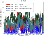
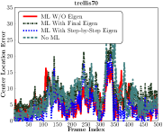
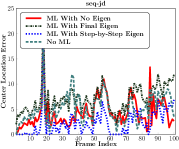
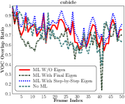
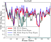
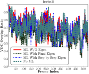

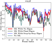
XI Comparison of different linear representations
We evaluate the performance of four types of linear representations including our linear representation with metric learning, our linear representation without metric learning, compressive sensing linear representation [7], and -regularized linear representation [6]. For a fair comparison, we utilize the raw pixel features which are the same as [7, 6]. Fig. 20 shows the performance of these four linear representation methods in CLE and VPR on four video sequences. Clearly, our linear representation with metric learning consistently achieves lower CLE (higher VOR) performance in most frames than the three other linear representations.
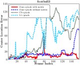
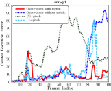


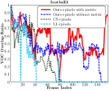
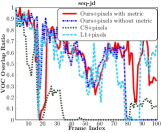

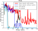
XII Evaluation of different sampling methods
We aim to examine the performance of the two sampling methods. Fig. 21 shows the experimental results of the two sampling methods in CLE and VOR on four video sequences. From Fig. 21, we can see that weighted reservoir sampling performs better than ordinary reservoir sampling.
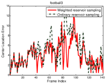

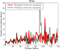
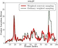

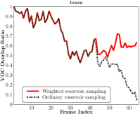


XIII Pedestrian identification
Based on Equ. (19), we perform the pedestrian identification task with two viewpoints. Fig. 22 shows the quantitative frame-by-frame identification results for five pedestrians with different viewpoints. Moreover, Figs. 23-31 display the tracking and identification results for six pedestrians on several representative frames. Clearly, our method is able to achieve a robust pedestrian identification performance in different cases.

(a)

(b)
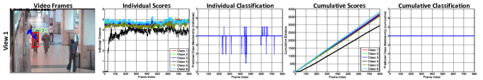
(c)
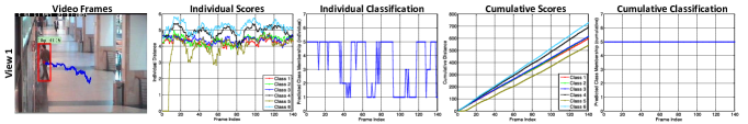
(d)

(e)


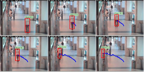
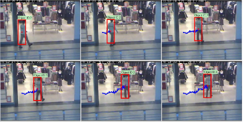


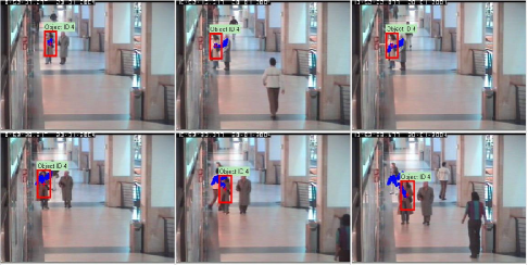
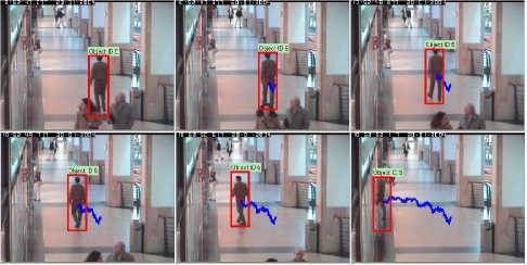

XIV Comparison with the state-of-the-art trackers
We report the quantitative tracking results of the eleven trackers in CLE and VOR over the eighteen video sequences. Figs. 32 and 33 plot the frame-by-frame CLEs and VORs (marked with the curves in different colors) obtained by the eleven trackers. From Figs. 32 and 33, we observe that the proposed tracking algorithm achieves the best tracking performance on most video sequences.
Moreover, we show the corresponding qualitative tracking results of the eleven trackers (highlighted by the bounding boxes in different colors) over the representative frames of the eighteen video sequences in Figs. 34–51. Clearly, it is seen from Figs. 34–51 that the proposed tracking algorithm obtains the most accurate tracking results in most cases.


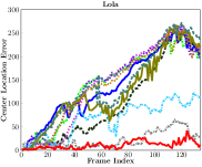


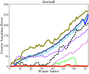
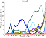
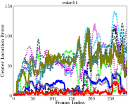
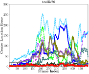
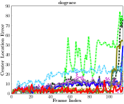
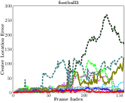
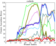
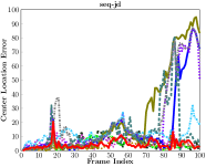
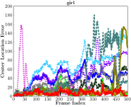

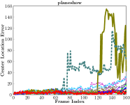
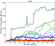
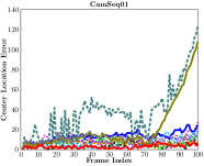
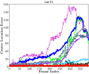


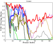


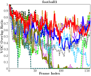
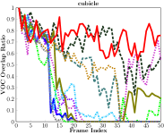

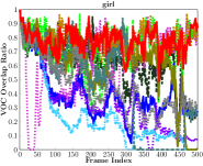


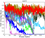

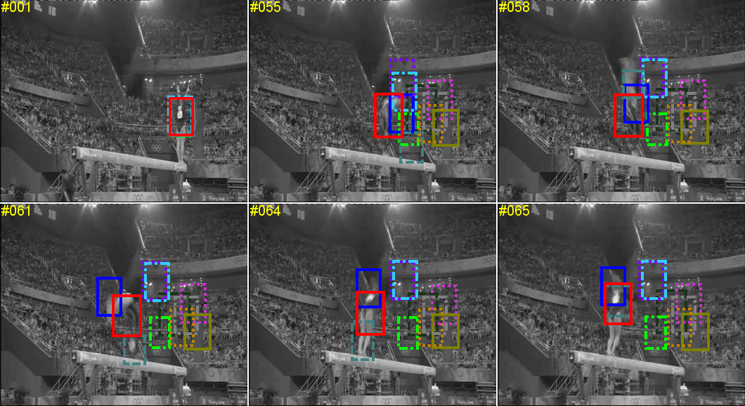


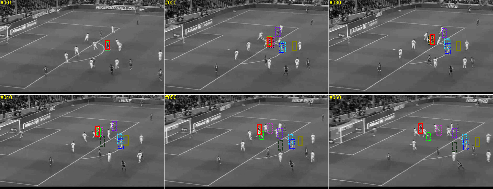


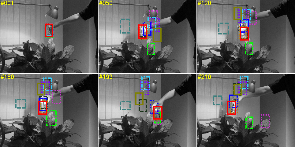


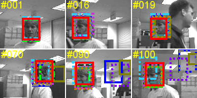

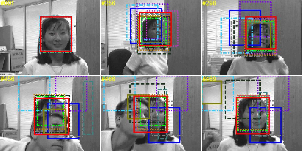


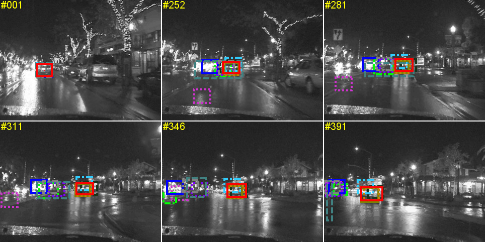
XV Discussion
Based on the obtained experimental results, we observe that the proposed tracking algorithm has the following properties. First, after the buffer size exceeds a certain value (around in our experiments), the tracking performance keeps stable with an increasing buffer size, as shown in Fig. 3. This is desirable since we do not need a large buffer size to achieve promising performance. Second, in contrast to many existing particle filtering-based trackers whose running time is typically linear in the number of particles, our method’s running time is sublinear in the number of particles, as shown in Fig. 3. Moreover, its tracking performance rapidly improves and finally converge to a certain value, as shown in Fig. 3. Third, as shown in Fig. 19 and Tab. VII, the performance of our metric learning with no eigendecomposition is close to that of computationally expensive metric learning with step-by-step eigendecomposition. Fourth, using the structured metric learning is capable of improving the tracking performance in CLE and VOR, as shown in Tab. V. That is because the structured metric learning encodes the underlying the structural interaction information on data samples, which plays an important role in robust visual tracking. Fifth, based on linear representation with metric learning, it performs better in tracking accuracy, as shown in Fig. 20. Sixth, it utilizes weighed reservoir sampling to effectively maintain and update the foreground and background sample buffers for metric learning, as shown in Fig. 21. Seventh, compared with other state-of-the-art trackers, it is capable of effectively adapting to complicated appearance changes in the tracking process by constructing an effective metric-weighted linear representation with weighed reservoir sampling, as shown in Fig. 32 and Tab. IV.