Adaptive stratified Monte Carlo algorithm for numerical computation of integrals

Abstract.

In this paper, we aim to compute numerical approximation integral by using an adaptive Monte Carlo algorithm. We propose a stratified sampling algorithm based on an iterative method which splits the strata following some quantities called indicators which indicate where the variance takes relative big values. The stratification method is based on the optimal allocation strategy in order to decrease the variance from iteration to another. Numerical experiments show and confirm the efficiency of our algorithm.

Keywords: Monte Carlo method, optimal allocation, adaptive method, stratification.

1. Introduction

This paper deals with adaptive Monte Carlo method (AMC) to approximate the integral of a given function $f$ on the hypercube $[0,1[^{d},d\in{\rm IN}^{*}$. The main idea is to guide the random points in the domain in order to decrease the variance and to get better results. The corresponding algorithm couples two methods: the optimal allocation strategy and the adaptive stratified sampling. In fact, it proposes to split the domain into separate regions (called mesh) and to use an iterative algorithm which calculates the number of samples in every region by using the optimal allocation strategy and then refines the parts of the mesh following some quantities called indicators which indicate where the variance takes a relative big values.

A usual technique for reducing the mean squared error of a Monte-Carlo estimate is the so-called stratified Monte Carlo sampling, which considers sampling into a set of strata, or regions of the domain, that form a partition (a stratification) of the domain (see [6] and the references therein for a presentation more detailed). It is efficient to stratify the domain, since when allocating to each stratum a number of samples proportional to its measure, the mean squared error of the resulting estimate is always smaller or equal to the one of the crude Monte-Carlo estimate. For a given partition of the domain and a fixed total number of random points, the choice of the number of samples in each stratum is very important for the results and precision. The optimal allocation strategy (see for instance [3] or [1]) allows to get the better distribution of the samples in the set of strata in order to minimize the variance. We give in the next section a brief summary of the this strategy which will be the basic tools of our adaptive algorithm.

In the other hand, it is important to stratify the domain in connection with the function $f$ to be integrated and to allocate more strata in the region where $f$ has larger local variations. Many research works propose multiple methods and technics to stratify the domain: [1] for the adaptive stratified sampling for Monte-Carlo integration of differentiable functions, [5] for the adaptive integration and approximation over hyper-rectangular regions with applications to basket option pricing, [4], ….

The paper is organized as follows. Section 2 describes the adaptive method. We begin by giving a summarize of the optimal allocation strategy and then describe the adaptive algorithm consisting in stratifying the domain. In section 3, we perform numerical investigations showing the powerful of the proposed adaptive algorithm.

2. Description of the adaptive algorithm

In this section, we will describe the AMC algorithm which is based on indicators to guide the repartition of the random points in the domain. In our algorithm, the indicators are based on an approximation of the variance expressed on different regions in the domain. We detect those where the indicators are bigger than their mean value up to a constant and we split them in small regions.

2.1. Optimal choice of the numbers of samples

Let $D=[0,1[^{d}$ be the unit hypercube of ${\rm IR}^{d}$, $d\in{\rm IN}^{*}$, and $f:D\rightarrow{\rm IR}$ a Lebesgue-integrable function. We want to estimate

$$\mathcal{I}(f)=\int_{D}f(x)d\lambda(x),$$

where $\lambda$ is the Lebesgue measure on ${\rm IR}^{d}$.

The classical MC estimator of $\mathcal{I}(f)$ is

$$\mathcal{\bar{I}}_{\text{MC}}(f)=\displaystyle\frac{1}{N}\sum_{i=1}^{N}f\circ U_{i},$$

where $U_{i},1\leq i\leq N$, are independent random variables uniformly distributed over $D$. $\mathcal{\bar{I}}_{\text{MC}}(f)$ is an unbiased estimator of $\mathcal{I}(f)$, which means that ${\mathrm{E}}[\mathcal{\bar{I}}_{\text{MC}}(f)]=\mathcal{I}(f)$. Moreover, if $f$ is square-integrable, the variance of $\mathcal{\bar{I}}_{\text{MC}}(f)$ is

$${\mathrm{Var}}(\mathcal{\bar{I}}_{\text{MC}}(f))=\displaystyle\frac{\sigma^{2}(f)}{N}$$

where

$$\sigma^{2}(f)=\displaystyle\int_{D}f(x)^{2}d\lambda(x)-\left(\displaystyle\int_{D}f(x)d\lambda(x)\right)^{2}.$$

Variance reduction techniques aim to produce alternative estimators having smaller variance than crude MC. Among these techniques, we focus on stratification strategy. The idea is to split $D$ into separate regions, take a sample of points from each such region, and combine the results to estimate $\mathcal{I}(f)$. Let $\{D_{1},\ldots,D_{p}\}$ be a partition of $D$. That is a set of sub-domains such that

$$D=\bigcup_{i=1}^{p}D_{i}\quad\text{and}\quad D_{i}\cap D_{j}=\emptyset\ \text{for}\ i\neq j.$$

We consider $p$ corresponding integers $n_{1},\ldots,n_{p}$. Here, $n_{i}$ will be the number of samples to draw from $D_{i}$. For $1\leq i\leq p$, let $a_{i}=\displaystyle\int_{D_{i}}d\lambda(x)$ be the measure of $D_{i}$ and $\mathcal{I}_{i}(f)=\displaystyle\int_{D_{i}}f(x)d\lambda(x)$ be the integral of $f$ over $D_{i}$. We have $\lambda(D)=\displaystyle\sum_{i=1}^{p}a_{i}$ and $\mathcal{I}(f)=\displaystyle\sum_{i=1}^{p}\mathcal{I}_{i}(f)$. Furthermore, for $1\leq i\leq p$, let $\pi_{i}=\displaystyle\frac{1_{D_{i}}}{a_{i}}\lambda$ be the density function of the uniform distribution over $D_{i}$ and consider a set of $n_{i}$ random variables $X^{(i)}_{1},\dots,X^{(i)}_{n_{i}}$ drawn from $\pi_{i}$. We suppose that the random variables $X^{(i)}_{j},1\leq j\leq n_{i},1\leq i\leq p$, are mutually independent.

For $1\leq i\leq p$, let $S_{i}$ be the MC estimator of $\mathcal{I}_{i}(f)$ defined by:

$$S_{i}=\displaystyle\frac{1}{n_{i}}\sum_{k=1}^{n_{i}}f\circ X^{(i)}_{k}.$$

Then, the integral $\mathcal{I}(f)$ can be estimated by:

$$\mathcal{\bar{I}}_{\text{SMC}}(f)=\displaystyle\sum_{i=1}^{p}a_{i}S_{i}=\displaystyle\sum_{i=1}^{p}\frac{a_{i}}{n_{i}}\sum_{k=1}^{n_{i}}f\circ X^{(i)}_{k}.$$

We call $\mathcal{\bar{I}}_{\text{SMC}}(f)$ the stratified Monte Carlo estimator of $\mathcal{I}(f)$. It is easy to show that $\mathcal{\bar{I}}_{\text{SMC}}(f)$ is an unbiased estimator of $\mathcal{I}(f)$ and, if $f$ is square-integrable, the variance of $\mathcal{\bar{I}}_{\text{SMC}}(f)$ is

$${\mathrm{Var}}(\mathcal{\bar{I}}_{\text{SMC}}(f))=\displaystyle\sum_{i=1}^{n_{i}}a_{i}^{2}\displaystyle\frac{\sigma^{2}_{i}(f)}{n_{i}}$$

where

$$\sigma^{2}_{i}(f)=\displaystyle\int_{D}f(x)^{2}d\pi_{i}(x)-\left(\int_{D}f(x)d\pi_{i}(x)\right)^{2},\quad\forall 1\leq i\leq p.$$

The choice of the integers $n_{i}$, $i=1,\ldots,p$ is crucial in order to reduce ${\mathrm{Var}}(\mathcal{\bar{I}}_{\text{SMC}}(f))$. A frequently made choice is proportional allocation which takes the number $n_{i}$ of points in each sub-domain $D_{i}$ proportional to its measure. In other words, if $N=\displaystyle\sum_{i=1}^{p}n_{i}$, then $n_{i}=Na_{i},i=1,\ldots,p$.

For this choice, we have

$${\mathrm{Var}}(\mathcal{\bar{I}}_{\text{MC}}(f))={\mathrm{Var}}(\mathcal{\bar{I}}_{\text{SMC}}(f))+\frac{1}{N}\sum_{i=1}^{p}a_{i}\left(\frac{\mathcal{I}_{i}(f)}{a_{i}}-\mathcal{I}(f)\right)^{2},$$

and hence, ${\mathrm{Var}}(\mathcal{\bar{I}}_{\text{SMC}}(f))\leq{\mathrm{Var}}(\mathcal{\bar{I}}_{\text{MC}}(f))$.

To get an even smaller variance, one can consider The optimal allocation which aims to minimize

$$V(n_{1},\ldots,n_{p})=\displaystyle\sum_{i=1}^{n_{i}}a_{i}^{2}\displaystyle\frac{\sigma^{2}_{i}(f)}{n_{i}},$$

as a function of $n_{1},\ldots,n_{p}$, with $N=\displaystyle\sum_{i=1}^{p}n_{i}$. Let

$$\delta=\displaystyle\frac{1}{N}\sum_{i=1}^{p}a_{i}\sigma_{i}(f).$$

Using the inequality of Cauchy-Schwarz, we have

$$V\left(\frac{a_{1}\sigma_{1}(f)}{\delta},\dots,\frac{a_{p}\sigma_{p}(f)}{\delta}\right) =\frac{1}{N}\left(\sum_{i=1}^{p}a_{i}\sigma_{i}(f)\right)^{2}$$

$$\leq\frac{1}{N}\left(\sum_{i=1}^{p}\frac{a_{i}^{2}\sigma_{i}(f)^{2}}{n_{i}}\right)\sum_{i=1}^{p}n_{i}$$

$$\leq V(n_{1},\ldots,n_{p}).$$

Hence, the optimal choice of $n_{1},\ldots,n_{p}$ is given by

$$n_{i}=\frac{a_{i}\sigma_{i}(f)}{\delta},\quad i=1,\dots,p.$$ (2.1)

In order to compute the number $n_{i}$ of random points in $D_{i}$ using (2.1), one can approximate $\sigma_{i}(f)$ by:

$$\bar{\sigma}^{2}_{i}(f)=\displaystyle\frac{1}{n_{i}}\sum_{j=1}^{n_{i}}(f\circ X^{(i)}_{j})^{2}-\Bigl{(}\frac{1}{n_{i}}\sum_{j=1}^{n_{i}}f\circ X^{(i)}_{j}\Bigr{)}^{2}.$$ (2.2)

For $1\leq i\leq p$, we will denote

$$\bar{n}_{i}=\displaystyle\frac{a_{i}\bar{\sigma}_{i}(f)}{\bar{\delta}}$$ (2.3)

where

$$\bar{\delta}=\displaystyle\frac{1}{N}\sum_{i=1}^{p}a_{i}\bar{\sigma}_{i}(f).$$ (2.4)

2.2. Description of the algorithm

The adaptive MC scheme aims to guide, for a fixed global number $N$ of random points in the domain $D$, the generation of random points in every sub-domain in order to get more precise estimation on the desired integration. It is based on an iterative algorithm where the mesh (repartition of the sub-domains in $D$) evolves with iterations. Let $L$ be the total number of desired iterations and $D^{\ell},1\leq\ell\leq L,$ be the corresponding mesh such that

$$D^{\ell}=\bigcup_{i=1}^{p_{\ell}}D^{\ell}_{i}\quad\text{and}\quad D^{\ell}_{i}\cap D^{\ell}_{j}=\emptyset\ \text{for}\ i\neq j,$$

where $p_{\ell}$ is the number of the sub-domains in $D^{\ell}$. We start the iterations with a subdivision of the domain $D^{1}=D$ using $p_{1}$ identical sub-cubes with given equal numbers of random points $n_{i,1}$ in each sub-domain $D^{1}_{i},i=1,\dots,n_{i,1}$, such that $N=\displaystyle\sum_{i=1}^{p_{1}}n_{i,1}$.

The main idea of the algorithm consists for every iteration $1\leq\ell\leq L$, to refine some region $D^{\ell}_{i}$, $1\leq i\leq p_{\ell}$, of the mesh $D^{\ell}$ where the function $f$ presents more singularities (big values of the variance) and hence must be better described. This technique is based on some quantities called indicators and denoted ${V}_{i,\ell}$ which give informations about the contribution of $D^{\ell}_{i}$ in the calculation of the variance of the MC method at this level, approximated by

$${V}_{\ell}=\displaystyle\sum_{i=1}^{p_{l}}{V}_{i,\ell}$$ (2.5)

where

$${V}_{i,\ell}=\displaystyle\frac{a_{i,\ell}^{2}\bar{\sigma}_{i,\ell}^{2}(f)}{\bar{n}_{i,\ell}}.$$ (2.6)

Our goal is to decrease ${V}_{\ell}$ during the iterations. Then, for every refinement iteration $\ell$ with a corresponding mesh $D^{\ell}$ and corresponding numbers $\bar{n}_{i,\ell}$, we calculate $\bar{\sigma}_{i,\ell}(f)$ and $\bar{\delta}_{\ell}$, and update $\bar{n}_{i,\ell}$ by using the optimal choice of the numbers of samples based on the formulas (2.2), (2.4) and (2.3) for all the sub-domains $D^{\ell}_{i},i=1,\dots,p_{\ell}$. For technical reason, we allow a minimal number, denoted by $M_{rp}$ (practically we choose $M_{rp}=2$), of random points in every sub-domain and then if $\bar{n}_{i,\ell}<M_{rp}$ we set $\bar{n}_{i,\ell}=M_{rp}$.
Next, we calculate the indicators ${V}_{i,\ell}$ and ${V}_{\ell}$, and then, we adapt the mesh $D^{\ell}$ to obtain the new one $D^{\ell+1}$. The chosen strategy of the adaptive method consists to mark the sub-domains $D^{\ell}_{i}$ such that

$${V}_{i,\ell}>C_{m}{V}^{mean}_{\ell},$$

where $C_{m}$ is a positive constant bigger than $1$ and ${V}^{mean}_{\ell}$ is the mean value of ${V}_{i,\ell}$ defined as

$${V}^{mean}_{\ell}=\displaystyle\frac{1}{p_{\ell}}\sum_{i=1}^{p_{l}}V_{i,\ell},$$ (2.7)

and to divide every marked sub-domains $D^{\ell}_{i}$ into small parts, four equal sub-squares for $d=2$ and eight equal sub-cubes for $d=3$, with equal number of random points in each part given by

$$\left\{\begin{array}[]{rcl}\vskip 6.0pt plus 2.0pt minus 2.0pt\displaystyle\max(\frac{\bar{n}_{i,\ell}}{4},M_{pr})\qquad\mbox{for }d=2\\ \displaystyle\max(\frac{\bar{n}_{i,\ell}}{8},M_{pr})\qquad\mbox{for }d=3.\end{array}\right.$$

Remark 2.1.

We stop the algorithm if the number of iterations reaches $L$ or if the calculated variance is smaller that a tolerance denoted by $\varepsilon$. We denote by $\ell_{\varepsilon}$ the stopping iteration level of the following algorithm which corresponds to a desired tolerance $\varepsilon$ or at maximum equals to $L$.

The algorithm can be described as following :

(Algo 1) : For a chosen $N$ with corresponding numbers $n_{i,1}$, and a given initial mesh $D^{1}$ with corresponding sub-domains $D^{1}_{i},i=1,\dots,p_{1}$,

Generate $n_{i,1},i=1,\dots,p_{1}$ random points $X^{i}_{j},j=1,\dots,n_{i,1}$ in every sub-domain  $D^{1}_{i}$.
set $\ell=1$.
calculate $V_{\ell}$ by using (2.5).
While $l{\leq}LorV_{\ell}\leq\varepsilon$
    calculate $\bar{\sigma}_{i,\ell}(f)$ and, $\bar{\delta}_{\ell}$ and  update $\bar{n}_{i,\ell},i=1,\dots,p_{\ell}$ by using (2.2), (2.4) and (2.3).
    Generate corresponding random points $X^{i}_{j},j=1,\dots,n_{i,l}$ in each sub-domain $D^{\ell}_{i},i=1,\dots,p_{\ell}$.
    calculate ${V}_{i,\ell},i=1,\dots,p_{l}$ and ${V}^{mean}_{\ell}$ by using (2.6) and (2.7).
    for ($i=1:p_{\ell}$)
        if ($V_{i,\ell}\geq C_{m}V^{mean}_{\ell}$)
            Divide the sub-domain $D_{i}^{\ell}$ in $m$ small parts ($m=4$ in 2D and $m=8$ in 3D).
            Associate to every one of this small parts the number of random points max($\displaystyle\frac{\bar{n}_{i,l}}{m},M_{pr}$).
            set $p_{\ell}=p_{\ell}+m$.
        end if
    end for
    $\ell=\ell+1$.
end loop
$\ell_{\varepsilon}=\ell-1$.
calculate the adapt MC approximation $\mathcal{I}_{AMC}=\displaystyle\sum_{i=1}^{p_{\ell_{\varepsilon}}}\frac{a_{i,\ell_{\varepsilon}}}{\bar{n}_{i,\ell_{\varepsilon}}}\sum_{k=1}^{n_{i,\ell_{\varepsilon}}}f\circ{X^{i}_{k}}$.

The previous algorithm calculate an approximation of ${\mathcal{I}}(f)$ with an adaptive Monte Carlo method. If we are interested by the numerical variance, we repeat the previous algorithm $N_{ess}$ times and approximate the ${\mathcal{I}}(f)$ by the corresponding mean value

$$\bar{\mathcal{I}}_{AMC}=\displaystyle\frac{1}{N_{ess}}\sum_{i=1}^{N_{ess}}{\mathcal{I}}^{i}_{AMC},$$

where ${\mathcal{I}}^{i}_{AMC}$ corresponds to the $i^{th}$ essay using (Algo 1).
The estimated variance will by given by the formula

$$V_{AMC}=\displaystyle\frac{1}{N_{ess}-1}\Big{(}\sum_{i=1}^{N_{ess}}({\mathcal{I}}^{i}_{AMC})^{2}-N_{ess}\,\bar{\mathcal{I}}_{AMC}^{2}\Big{)}.$$

In fact, it is useless to repeat the (Algo 1) $N_{ess}$ times to calculate $\bar{\mathcal{I}}_{AMC}$ and $V_{AMC}$, and it is expensive for the CPU time. We can reduce the coast by running (Algo 1) one time to define the mesh and to get ${\mathcal{I}}^{1}_{AMC}$ and then, we use the corresponding sub-domains $D^{\ell_{\varepsilon}}_{i},i=1,\dots,p_{\ell_{\varepsilon}}$ with the corresponding number of random points $n_{i,\ell_{\varepsilon}},i=1,\dots,\ell_{\varepsilon}$ to perform the rest of calculations ($N_{ess}-1$ essays). The corresponding algorithm can be describe as follow :

(Algo 2) :

Call algorithm (Algo 1) to define the mesh $D^{\ell_{\varepsilon}}_{i},i=1,\dots,p_{\ell_{\varepsilon}}$ and calculate $\mathcal{I}^{1}_{AMC}$
Set $n_{e}=2$
While  $n_{e}{\leq}N_{ess}$
    Generate corresponding random points $X^{i}_{j},j=1,\dots,n_{i,\ell_{\varepsilon}}$ in each sub-domain $D^{\ell_{\varepsilon}}_{i},i=1,\dots,p_{\ell_{\varepsilon}}$.
    Calculate $\mathcal{I}^{n_{e}}_{AMC}=\displaystyle\sum_{i=1}^{p_{\ell_{\varepsilon}}}\frac{a_{i,\ell_{\varepsilon}}}{\bar{n}_{i,\ell_{\varepsilon}}}\sum_{k=1}^{n_{i,\ell_{\varepsilon}}}f\circ{X^{i}_{k}}$
    Set $n_{e}=n_{e}+1$
end loop calculate
$\bar{\mathcal{I}}_{AMC}=\displaystyle\frac{1}{N_{ess}}\sum_{i=1}^{N_{ess}}\mathcal{I}^{i}_{AMC}$ calculate
$V_{AMC}=\displaystyle\frac{1}{N_{ess}-1}\Big{(}\sum_{i=1}^{N_{ess}}({\mathcal{I}}^{i}_{AMC})^{2}-N_{ess}\,\bar{\mathcal{I}}_{AMC}^{2}\Big{)}$

3. Numerical experiments

In this section, we perform in MATLAB several numerical experiments to validate our approach and we compare between the MC and AMC methods.

3.1. 2D validations

We consider the unit square $D=[0,1[^{2}$, $C_{m}=2$, $M_{pr}=2$ and $\ell_{\varepsilon}=L$. The initial mesh is constituted by a regular partition with $N_{0}=4$ segments in every side of $D^{1}=D$ (see figure 1).

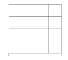
Figure 1. Initial partition $D^{1}_{i},i=1,\dots,p_{1}$ ($p_{1}=16$)with $N_{0}=4$.

In this section, we show two particular cases of the function $f$. The first treats an integrable but not continuous function which presents a discontinuity along the border of the unit disc. The second one treats a function concentrated in a part of $D$ and vanishes in the rest on this domain. Both examples show the powerful of the proposed AMC method.

3.1.1. First test case

For the first test case, we consider the function $f_{c}$ given on $D$ by

$$f_{c}(x,y)=\left\{\begin{array}[]{rcl}1&&\mbox{ if }x^{2}+y^{2}\leq 1\\ 0&&\mbox{ elsewhere. }\end{array}\right.$$

The exact integration of $f_{c}$ over $D$ is equal to

$$I=\displaystyle\int_{D}f_{c}(x,y)dxdy=\displaystyle\frac{\pi}{4},$$

which is the quarter of the surface of the unit disc.

We begin the numerical tests with the algorithm (Alog 1). Figures 3-7 show for $N=10000$ and $L=6$ the evolution of the mesh and the repartition of the random points during the iterations. We remark that this points are concentrated around the curve $x^{2}+y^{2}=1$ where the function $f_{c}$ represents a singularity.

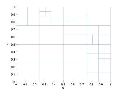
Figure 2. Mesh for the second iteration.

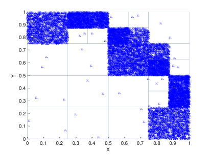
Figure 3. repartition of the points (second iteration).

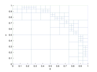
Figure 4. Mesh for the fourth iteration.

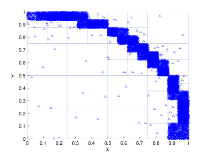
Figure 5. repartition of the points (fourth iteration).

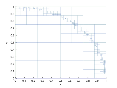
Figure 6. Mesh for the sixth iteration.

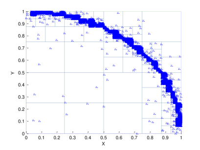
Figure 7. repartition of the points (sixth iteration).

Figure 9 shows a comparison in logarithmic scale of the relative errors ($I=\displaystyle\frac{\pi}{4}$)

$$E_{MC}=\displaystyle\frac{I-I_{MC}}{I}$$

corresponding to the MC method and

$$E_{AMC}=\displaystyle\frac{I-I_{AMC}}{I}$$

corresponding to the AMC method with respect to the number of random points $N$ where the total number of the iteration $L=4$. As we can see in figure 9, the AMC method is more precise than the MC method. Still we have to compare the efficiency of the AMC method with respect to the CPU time of computation. In fact, figure 9 shows that for the considered $N$, the corresponding CPU times for the AMC are smaller from those with MC. In particular, the MC method gives for $N=10^{7}$ an error of $E_{MC}=0.00052$ with a CPU time of $0.44s$, but the AMC gives for $N=10^{6}$ an error of $E_{AMC}=0.00008$ with a CPU time of $0.4s$. Hence, the powerful of the AMC method. It is also clear that to get more precision with the AMC method, we can increase the number of iterations $L$.

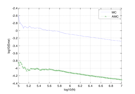
Figure 8. First test case: $E_{MC}$ and $E_{AMC}$ with respect to $N$ in logarithmic scale.

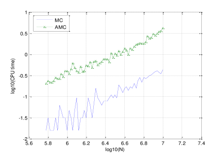
Figure 9. First test case: CPU time of the MC and AMC methods with respect to $N$ in logarithmic scale.

Next, we consider the algorithm (Algo 2) with $N_{ess}=100$, $L=4$.

Figure 11 shows the comparison of the estimated variance between the classical Monte Carlo ($V_{MC}$) and adaptive Monte Carlo method ($V_{AMC}$) in logarithmic scale. As the adaptive algorithm consists to minimize the variance, it is clear in this figure that the goal is attended. Figure 11 shows in logarithmic scale the efficiency of the MC and AMC methods versus the number of random points $N$ by using the following formulas (see [2])

$$E^{eff}_{MC}=\displaystyle\frac{1}{T_{MC}*V_{MC}}$$

and

$$E^{eff}_{AMC}=\displaystyle\frac{1}{T_{AMC}*V_{AMC}},$$

where $T_{MC}$ and $T_{AMC}$ are respectively the CPU time of the MC and AMC methods. It is clear that the efficiency of the AMC method is more important than the MC method.

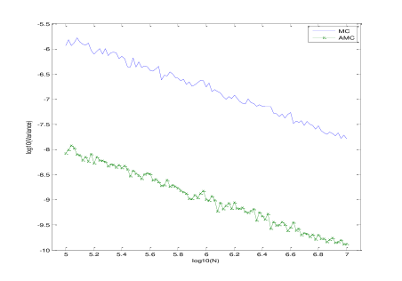
Figure 10. First test case: Estimated variances $V_{MC}$ and $V_{AMC}$ with respect to $N$ in logarithmic scale.

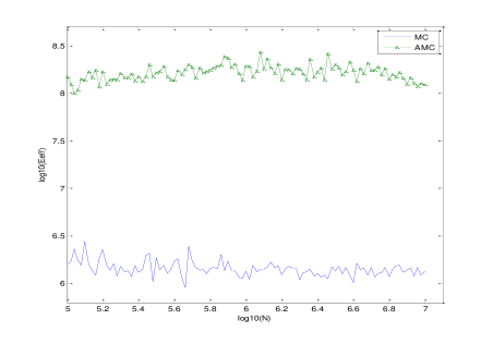
Figure 11. First test case: Efficiencies $E^{eff}_{MC}$ and $E^{eff}_{AMC}$ with respect to $N$ in logarithmic scale.

3.1.2. Second test case

In this case, we consider the function

$$f_{2,g}(x,y)=e^{-\alpha(x^{2}+y^{2})},$$

where $\alpha$ is a real positive parameter. We begin the adaptive algorithm with the same initial mesh as the previous case and we choose $N=10000$. Figures 15-15 show for $L=6$ the meshes and random points repartition with respect to $\alpha$. When $\alpha$ increase, the mesh and the random points follow the function $f_{2,g}$ and focus more and more around the origin of axis.

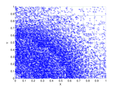
Figure 12. AMC mesh, $\alpha=-5$.

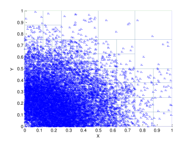
Figure 13. AMC mesh $\alpha=-10$.

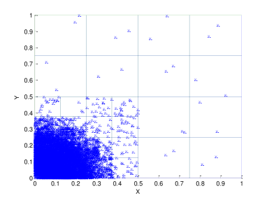
Figure 14. AMC mesh $\alpha=-50$.

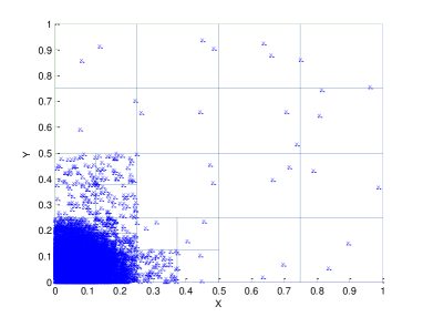
Figure 15. AMC mesh $\alpha=-100$.

Figure 17 shows for $\alpha=-50$, $N_{ess}=100$ and $L=4$, the comparison of the estimated variance between MC and AMC methods with respect to $N$ in logarithmic scale. Figure 17 shows in logarithmic scale the efficiency of the MC and AMC methods versus the number of points $N$. One more time, it is clear that the efficiency of the AMC method is more important than the MC one.

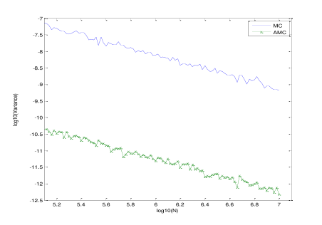
Figure 16. Second test case ($\alpha=-50$): Estimated variances $V_{MC}$ and $V_{AMC}$ with respect to $N$ in logarithmic scale.

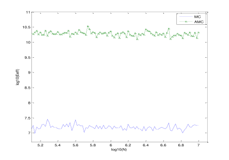
Figure 17. Second test case ($\alpha=-50$): Efficiencies $E^{eff}_{MC}$ and $E^{eff}_{AMC}$ with respect to $N$ in logarithmic scale.

3.2. 3D validations

In this section, we consider the unit cube $D=[0,1[^{3}$. We consider the function

$$f_{3,g}(x,y)=e^{-\alpha(x^{2}+y^{2}+z^{2})},$$

where $\alpha$ is a real positive parameter. The initial mesh is constituted by a regular partition with $N_{0}=4$ segments in every side of $D^{1}=D$. Figure 18 shows the repartition of the random points for $\alpha=-50$, $L=6$ and $N=10000$.

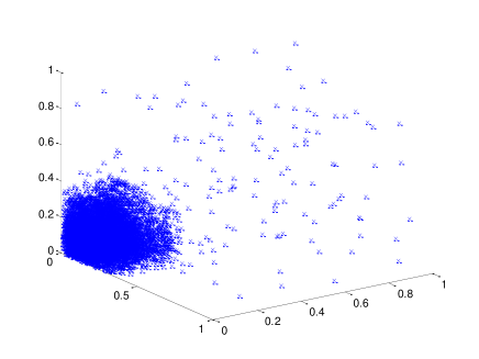
Figure 18. Mesh Gaussian for $\alpha=-50$.

As for the previous case, figure 20 shows for $N_{ess}=100$ and $L=4$, the comparison of the estimated variance between MC and AMC methods with respect to $N$ in logarithmic scale. Figure 20 shows in logarithmic scale the efficiency of the MC and AMC methods versus the number of points $N$. We can deduce the same remark for the efficiency of the AMC method in dimension three.

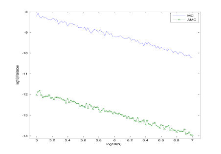
Figure 19. 3D test case ($\alpha=-50$): Estimated variances $V_{MC}$ and $V_{AMC}$ with respect to $N$ in logarithmic scale.

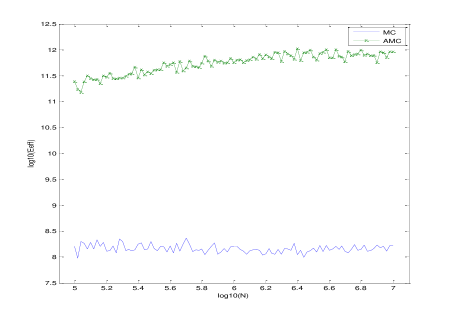
Figure 20. 3D test case ($\alpha=-50$): Efficiencies $E^{eff}_{MC}$ and $E^{eff}_{AMC}$ with respect to $N$ in logarithmic scale.

Acknowledgments We are grateful to my colleague Rami El Haddad for all the help given by him.

References

- [1] A. Carpentier and R. Munos, Finite-time analysis of stratified sampling for monte carlo, In Advances in Neural Information Processing Systems, (2011).
- [2] P. L’Ecuyer, Efficiency Improvement and Variance Reduction, Proceedings of the 1994 Winter Simulation Conference, Dec. (1994), 122–132.
- [3] P. Étoré and B. Jourdain, Adaptive optimal allocation in stratified sampling methods, Methodol. Comput. Appl. Probab., 12(3), (2010), 335–360.
- [4] P. Fearnhead and B. M. Taylor, An Adaptive Sequential Monte Carlo Sampler, Bayesian Anal., 8, (2), (2013), 411–438.
- [5] C. De Luigi and S. Maire, Adaptive integration and approximation over hyper-rectangular regions with applications to basket option pricing, Monte Carlo Methods Appl., 16, (2010), 265–282.
- [6] P. Glasserman, Monte Carlo methods in financial engineering, pringer Verlag, (2004). ISBN 0387004513.