Fractal and Small-World Networks Formed by Self-Organized Critical Dynamics

Abstract

We propose a dynamical model in which a network structure evolves in a self-organized critical (SOC) manner and explain a possible origin of the emergence of fractal and small-world networks. Our model combines a network growth and its decay by failures of nodes. The decay mechanism reflects the instability of large functional networks against cascading overload failures. It is demonstrated that the dynamical system surely exhibits SOC characteristics, such as power-law forms of the avalanche size distribution, the cluster size distribution, and the distribution of the time interval between intermittent avalanches. During the network evolution, fractal networks are spontaneously generated when networks experience critical cascades of failures that lead to a percolation transition. In contrast, networks far from criticality have small-world structures. We also observe the crossover behavior from fractal to small-world structure in the network evolution.

I Introduction

Complex systems consisting of discrete elements and their pair interactions can be described by networks. Many of large-scale networks representing complexity of the real world are known to have common properties in their topology Albert02 ; Dorogovtsev03 ; Cohen10 , such as the scale-free property Barabasi99 , degree correlations Newman02 ; Newman03 , or community structures Girvan02 . In particular, structures of real-world networks are classified into two types from a viewpoint of the relation between the number of nodes and the path length, namely small-world structures Watts98 and fractal structures Song05 . For a small-world network, the average path length $\langle l\rangle$ is extremely small comparing to the network size $N$ and increases at most logarithmically with $N$, i.e., $\langle l\rangle\propto\log N$. Numerous real-world complex networks possess the small-world property Montoya02 ; Amaral00 ; Bassett06 ; Humphries08 . On the other hand, a network is called fractal if the relation $N_{\text{B}}(l_{\text{B}})\propto l_{\text{B}}^{-d_{\text{B}}}$ holds, where $N_{\text{B}}(l_{\text{B}})$ is the minimum number of subgraphs of diameter less than $l_{\text{B}}$ required to cover the network and $d_{\text{B}}$ is the fractal dimension Song05 . Since this relation at $l_{\text{B}}\sim\langle l\rangle$ suggests the power-law scaling $\langle l\rangle\propto N^{1/d_{\text{B}}}$ Kawasaki10 , the fractal nature seems to conflict with the small-world property. Nevertheless, real complex networks that are small world in the sense of $\langle l\rangle\propto\log N$ often satisfy the fractal scaling $N_{\text{B}}(l_{\text{B}})\propto l_{\text{B}}^{-d_{\text{B}}}$, as observed in the world-wide web, actor networks, protein interaction networks, cellular networks Song05 , power-grid networks Csanyi04 , and software networks Concas06 ; Myers03 . This apparent inconsistency can be reconciled by taking into account a structural crossover from fractal to small-world scaling associated with the change in length scale Kawasaki10 .

It is well understood that the small-world property arises from the existence of short-cut edges Watts98 . Only a tiny amount of short-cut edges added into a non-small-world network drastically reduces the average path length. In contrast, the microscopic mechanism of the emergence of fractality in complex networks still remains unclear though fractal networks and their relation to the scale-free property have been extensively studied Song05 ; Kawasaki10 ; Cohen04 ; Goh06 ; Song06 ; Rozenfeld07 ; Song07 ; Furuya11 ; Sun14 . It is thus also not understood why there exist small-world and fractal networks in the real world and how fractal networks crossover to small-world ones. In order to deal with these problems, it is significant to remind that many conventional fractal objects embedded in the Euclidean space are formed by dynamics exhibiting self-organized criticality Bak87 ; Bak93 ; Markovic14 ; Drossel92 ; Takayasu92 ; Rinaldo93 ; Sapoval04 . In self-organized critical (SOC) dynamics, a system approaches spontaneously a critical point without tuning external parameters and fluctuates around the critical state due to the instability of the critical or near-critical states. One of the remarkable features of SOC dynamics is that stationary fluctuations around criticality are accompanied by intermittent, avalanche-like bursts of some sort of dynamical quantities, in which the avalanche size distribution obeys a power law. It is natural to consider that fractal complex networks are also formed by SOC dynamics.

SOC dynamics on static complex networks have been extensively studied in previous works Markovic14 ; deArcangelis02 ; Moreno02 ; Goh03 ; Masuda05 ; Lin05 ; Pellegrini07 ; Luque08 ; Bhaumik13 ; Watanabe14 ; Noel14 . However, for the construction of fractal networks through SOC dynamics, we need to consider the interplay between internal dynamics and the network topology Gross08 ; Aoki12 ; Shimada14 , by which the network evolution itself displays SOC characteristics. There have been many models of network evolution driven by internal dynamics related to self-organized criticality, such as models based on the Bak-Sneppen dynamics Christensen98 ; Slanina99 ; Garlaschelli07 , other models of ecological systems Guill08 , models related to the sandpile dynamics Peixoto04 ; Peixoto08 ; Fronczak06 , a model describing the motion of solar flares Hughes03 , and rewiring models based on state changes of nodes or edges Bornholdt00 ; Rybarsch14 ; Bianconi04 ; Shin06 . Although these models generate nontrivial networks through the couplings to internal dynamics, it is difficult to say that fractal networks are formed by SOC dynamics in these models because of the lack of intermittent, avalanche-like behavior of network structures Christensen98 ; Bornholdt00 ; Rybarsch14 , the necessity of parameter tuning for criticality Bianconi04 ; Garlaschelli07 , or the absence of fractality in generated networks Slanina99 ; Hughes03 ; Bianconi04 ; Peixoto04 ; Peixoto08 ; Fronczak06 ; Shin06 ; Guill08 .

In this paper, we present a model of fractal networks formed by SOC dynamics. Taking into account the evolution of real networks, the network instability required for SOC dynamics is realized by overload failures of nodes. In general, when the size of a functional network becomes large, the probability that all nodes in the network can escape failures decreases. Failure(s) on a single or a few nodes can cause a cascade of overload failures, and the network decays into smaller ones. Our model combines a network growth by introducing new nodes and its decay due to the instability of large grown networks against cascading overload failures. It is numerically demonstrated that the present dynamical system exhibits self-organized criticality and the network evolution generates both fractal and small-world networks. Furthermore, the crossover behavior from fractal to small-world structure has been observed in SOC dynamics.

The rest of this paper is organized as follows. In Sect. 2, we formulate the model combining a network growth with cascading overload failures induced by fluctuating loads. Our numerical results are presented in Sect. 3. In this section, we show the time development of several measures describing the network structure, SOC character of the dynamics, and the fractal and small-world properties of networks generated in SOC dynamics. Section 4 is devoted to the summary.

II Model

II.1 Network instability — Cascading overload failures

In the present work, the instability required to construct an SOC model is realized by cascading overload failures in large networks. Our daily life is supported by various functional networks, such as power grids, computer networks, the world-wide web, etc. Functions of networks are achieved by some sort of flow which plays, at the same time, a role of loads in the network. The load on a node usually fluctuates temporally and its instantaneous value exceeding the allowable range causes a failure of node. This overload failure may induce a cascade of subsequent failures which reduces, sometimes greatly, the network size. Such cascades of failures provide the instability of networks. Recently, the robustness of a network against cascading overload failures induced by temporally fluctuating loads has been studied Mizutaka15 , This study employs the random walker model proposed by Kishore et al.Kishore11 ; Kishore12 , in which fluctuating loads are described by random walkers moving on a network. Since our model is based on the study by Ref. References, we briefly review this work.

In the random walker model Kishore11 ; Kishore12 ; Mizutaka13 , we consider $W_{0}$ non-interacting random walkers moving on a connected and undirected network with $M_{0}$ edges. Walkers on a node represent the temporally fluctuating load imposed on the node. Since the stationary probability $p_{k}$ to find a walker on a node of degree $k$ is given by $p_{k}=k/2M_{0}$ Noh04 , the probability that there exist $w$ walkers on the degree-$k$ node is presented by

$$h_{k}(w)=\binom{W_{0}}{w}p_{k}^{w}{(1-p_{k})}^{W_{0}-w}.$$ (1)

This binomial distribution gives the average load on the degree-$k$ node as $\langle w\rangle_{k}=W_{0}p_{k}$ and the standard deviation $\sigma_{k}=\sqrt{\langle w\rangle_{k}(1-p_{k})}$. It is then natural to define the capacity of a node of degree $k$ as

$$q_{k}=\langle w\rangle_{k}+m\sigma_{k},$$ (2)

where $m$ is a real positive parameter and characterizes the tolerance of the node to load. A node is considered to fail if the number of walkers $w$ on the node exceeds this capacity. Therefore, the probability $F_{W_{0}}(k)$ that a node of degree $k$ experiences an overload failure is calculated by summing up the distribution function $h_{k}(w)$ over $w$ larger than $q_{k}$. Using the regularized incomplete beta function $I_{x}(a,b)$ for this summation Abramowitz64 , the overload probability is expressed as Kishore11

$$F_{W_{0}}(k)=I_{k/2M_{0}}(\lfloor q_{k}\rfloor+1,W_{0}-\lfloor q_{k}\rfloor),$$ (3)

where the floor function $\lfloor x\rfloor$ represents the greatest integer less than or equal to $x$.

Applying the above idea of the overload probability, a cascade of failures starting with a specific large network can be described as follows Mizutaka15 .

• Prepare an initial connected, undirected, and uncorrelated network $\mathcal{G}_{0}$ with $N_{0}$ nodes and $M_{0}$ edges, in which $W_{0}$ random walkers exist, where $W_{0}$ is chosen so as to be proportional to $M_{0}$. In addition, determine the capacity $q_{k}$ of each node by Eq. (2).

• At each time step $\tau$, assign $W_{\tau}$ random walkers to the network $\mathcal{G}_{\tau}$ at step $\tau$, where the total load $W_{\tau}$ is given by

  $$W_{\tau}=W_{0}\left(\frac{M_{\tau}}{M_{0}}\right)^{r}.$$ (4)

  Here $M_{\tau}$ is the total number of edges in the network $\mathcal{G}_{\tau}$ and $r$ is a real positive parameter.

• Calculate the overload probability of every node, and remove nodes from $\mathcal{G}_{\tau}$ with this probability.

• Repeat (ii) and (iii) until no node is removed in the procedure (iii).

The reduction of the total load in the procedure (ii) corresponds to actual cascades of failures during which the total load is reduced to some extent to prevent the breakdown of the network function. We call the exponent $r$ in Eq. (4) the load reduction parameter hereafter. It should be emphasized that the overload probability in the procedure (iii) cannot be calculated by Eq. (3) with $W_{0}$ replaced by $W_{\tau}$ for the following two reasons. First, the degree $k$ of a node in the network $\mathcal{G}_{\tau}$ is not the same with its initial degree $k_{0}$. The capacity of a node is determined by the initial degree $k_{0}$, while the probability to find a walker on this node is proportional to the present degree $k$. Thus, the overload probability depends on both $k$ and $k_{0}$. Secondly, the network $\mathcal{G}_{\tau}$ is not necessarily connected, though the initial network $\mathcal{G}_{0}$ is connected. If $\mathcal{G}_{\tau}$ is not connected, $W_{\tau}$ random walkers are distributed to each component in proportion to the number of edges in the component, before starting the next cascade step. Taking into account these remarks and the fact that random walkers cannot jump to other components, the overload probability of a node of degree $k$, whose initial degree is $k_{0}$, in the $\alpha$-th component of $\mathcal{G}_{\tau}$ is given by

$$F_{W_{\tau}^{\alpha}}(k_{0},k)=I_{k/2M_{\tau}^{\alpha}}\left(\lfloor q_{k_{0}}\rfloor+1,W_{\tau}^{\alpha}-\lfloor q_{k_{0}}\rfloor\right),$$ (5)

where $M_{\tau}^{\alpha}$ is the number of edges in the $\alpha$-th component of $\mathcal{G}_{\tau}$ and $W_{\tau}^{\alpha}=W_{\tau}M_{\tau}^{\alpha}/M_{\tau}$ is the load assigned to the $\alpha$-th component. Since $k$ is always equal to $k_{0}$ and the network $\mathcal{G}_{\tau}$ is connected at $\tau=0$, $F_{W_{\tau}^{\alpha}}(k_{0},k)$ at $\tau=0$ coincides with $F_{W_{0}}(k)$ given by Eq. (3). Thus, Eq. (5) is a general form of the overload probability for $\tau\geq 0$.

The relative size $S_{\text{f}}$ of the giant component in the network $\mathcal{G}_{\text{f}}$ at the final stage of the cascade process is an important quantity to evaluate the robustness of networks against cascading overload failures. This quantity $S_{\text{f}}$ can be calculated by combining the generating function method Newman01 and the master equation for the probability $\Pi_{\tau}(k_{0},k)$ that a node in $\mathcal{G}_{\tau}$ has the present degree $k$ and the initial degree $k_{0}$, without simulating numerically the cascade process (i)–(iv) Mizutaka15 . By means of this method, it has been clarified that there exists a threshold value of the load reduction parameter $r_{\text{c}}(N_{0})$ above which $S_{\text{f}}$ becomes finite and below which $S_{\text{f}}=0$ and $r_{\text{c}}(N_{0})$ for $N_{0}\to\infty$ provides a percolation transition by cascading overload failures Mizutaka15 . The critical property of $\mathcal{G}_{\text{f}}$ at $r=r_{\text{c}}$ has also been confirmed by the fractality of the giant component in $\mathcal{G}_{\text{f}}$. These facts will be closely related to the results of the present work. However, in the case that the structure and node capacities of a network with which the cascade starts depend on results of cascading failures occurring in the past, as in the model of this work, it is unfortunately impossible to apply the method utilizing the generating function. In such a case, we need to simulate numerically the process (i)–(iv) to find the final network state after a cascade.

II.2 Network evolution

The basic idea of our dynamical model is to combine the growth of a network and its decay into smaller ones by cascading overload failures. The overload probability $F_{W_{0}}(k)$ given by Eq. (3) is almost independent of $M_{0}$ if $W_{0}\propto M_{0}$. However, the probability that the first failures inducing a cascade of subsequent failures occur in the network increases with the network growth. Thus, we expect that the network cannot grow infinitely and its size fluctuates around a certain value. Since our model includes two different types of dynamics, i.e., growth and cascade of failures, in order to distinguish them clearly, a time step of the network growth is hereafter denoted by $t$ in parentheses and a cascade step by subscript $\tau$. The concrete algorithm of the network evolution in our model is then given as follows:

• Start with a small and connected network $\mathcal{G}(0)$ with $N_{\text{ini}}$ nodes and $M_{\text{ini}}$ edges, in which $W_{\text{ini}}$ random walkers exist. $W_{\text{ini}}$ is set as $W_{\text{ini}}=aM_{\text{ini}}$, where $a$ is a positive constant. The capacities of the nodes in $\mathcal{G}(0)$ are calculated by Eq. (2).

• At every time step $t\geq 1$, add a new node with $\mu$ edges, where $\mu$ is in the range of $2\leq\mu\leq N_{\text{ini}}$, and connect the new node to $\mu$ different nodes selected randomly from the network $\mathcal{G}(t-1)$ at time $t-1$. Let $\mathcal{G}_{0}(t)$ be the network at this stage.

• Place $W_{0}(t)=aM_{0}(t)$ random walkers on the network $\mathcal{G}_{0}(t)$, where $M_{0}(t)$ is the number of edges in $\mathcal{G}_{0}(t)$, and calculate the capacity of the new node by using Eq. (2) with $k$ replaced by $\mu$ and for the total load $W_{0}(t)$.

• Perform cascading overload failures starting with $\mathcal{G}_{0}(t)$ in accordance with the process (i)–(iv) described in Sect. II.1. In this cascade process, isolated zero-degree nodes generated by the elimination of all their adjacent nodes, in addition to the overloaded nodes themselves, are removed from the system. Let $\mathcal{G}(t)$ be the resultant network after completing the cascade.

• Repeat the procedure from (2) to (4) for a sufficiently long period.

We should make several remarks concerning the above algorithm. In the procedure (2), the number of edges $\mu$ of a newly added node must be larger than $2$. Otherwise, once the network is divided into disconnected components by cascading failures, components never merge. The network after a long time becomes an assembly of a large number of small graphs. Thus, the dynamical system has a qualitatively different property from that for $\mu\geq 2$. It should be also emphasized that the network $\mathcal{G}_{0}(t)$ is not necessarily connected. If $\mathcal{G}_{0}(t)$ consists of plural components, the total load $W_{0}(t)$ is distributed to each component in the same way as the case of cascading failures. Namely, the number of walkers in the $\alpha$-th component is allocated by

$$W_{0}^{\alpha}(t)=W_{0}(t)\left[\frac{M_{0}^{\alpha}(t)}{M_{0}(t)}\right]=aM_{0}^{\alpha}(t),$$ (6)

where $M_{0}^{\alpha}(t)$ is the number of edges in the $\alpha$-th component of $\mathcal{G}_{0}(t)$. The calculation of the new-node capacity in the procedure (3) is actually done by using $W_{0}^{\alpha}(t)$, because random walkers cannot move to other components. The capacity of the node that is introduced at time $t$ and embedded in the $\alpha$-th component is then presented by

$$q^{\alpha}(t)=\langle w\rangle_{\mu}+m{\sigma}_{\mu}^{\alpha},$$ (7)

where $\langle w\rangle_{\mu}=W_{0}^{\alpha}(t)p_{\mu}^{\alpha}=a\mu/2$, $\sigma_{\mu}^{\alpha}=\sqrt{\langle w\rangle_{\mu}(1-p_{\mu}^{\alpha})}$, and $p_{\mu}^{\alpha}=\mu/2M_{0}^{\alpha}(t)$. Once the node capacity is determined, the value of $q$ never changes until the node is eliminated.

The process of cascading overload failures in the procedure (4) basically follows the steps (i)–(iv) in Sect. II.1 with replacing $\mathcal{G}_{0}$, $N_{0}$, $M_{0}$, and $W_{0}$ by $\mathcal{G}_{0}(t)$, $N_{0}(t)$, $M_{0}(t)$, and $W_{0}(t)$, respectively, where $N_{0}(t)$ is the number of nodes in $\mathcal{G}_{0}(t)$. In addition to the possibility of $\mathcal{G}_{0}(t)$ being disconnected, there are two other differences in the detailed treatment of the cascade process. Firstly, the overload probability of a node cannot be written as Eq. (5). This is because the node capacity given by Eq. (7) depends on when the node was introduced in the system. Thus, the overload probability of the node $i$ at cascade step $\tau$ is written as

$$F_{W_{\tau}^{\alpha}(t)}(i)=I_{k_{i}/2M_{\tau}^{\alpha}(t)}\left(\lfloor q^{\beta}(t_{i})\rfloor+1,W_{\tau}^{\alpha}(t)-\lfloor q^{\beta}(t_{i})\rfloor\right),$$ (8)

where $k_{i}$ is the degree of the node $i$, $t_{i}$ is the time at which the node $i$ was introduced, $\alpha$ and $\beta$ are the indices of the components to which the node $i$ belongs at the present cascade step $\tau$ and at $t_{i}$, respectively, and $q^{\beta}(t_{i})$ is presented by Eq. (7). The symbols $W_{\tau}^{\alpha}(t)$ and $M_{\tau}^{\alpha}(t)$ represent the number of random walkers and number of edges in the $\alpha$-th component of $\mathcal{G}_{\tau}(t)$, where $\mathcal{G}_{\tau}(t)$ is the network at the step $\tau$ of the cascade starting with $\mathcal{G}_{0}(t)$. The second difference is in the load reduction scheme during the cascade. In Sect. II.1, the total number of random walkers is reduced in accordance with the reduction of the network size during the cascade, as expressed by Eq. (4), to prevent the breakdown of the network function. It is actually difficult to reduce quickly the total load when the network size becomes large. Taking into account such realistic situations of cascading failures, the load reduction parameter $r$ characterizing how quickly the total load is reduced with the reduction of the network size should decrease with $N_{0}(t)$. Therefore, the total load during the cascade is reduced according to

$$W_{\tau}(t)=W_{0}(t)\left[\frac{M_{\tau}(t)}{M_{0}(t)}\right]^{r[N_{0}(t)]},$$ (9)

where $M_{\tau}(t)$ is the number of edges in $\mathcal{G}_{\tau}(t)$ and $r[N_{0}(t)]$ is a decreasing function of $N_{0}(t)$. Since large-scale cascades are more likely to occur if $r$ is small, the property that $r[N_{0}(t)]$ decreases with $N_{0}(t)$ prevents the network from growing too large.

If all nodes are eliminated from the system in the procedure (4), the network $\mathcal{G}(t)$ is reset to $\mathcal{G}(0)$ and continue the network evolution from the procedure (2). In the present model, the time scale of cascades measured by the step $\tau$ is assumed to be much faster than that of the network growth measured by the step $t$, and the relaxation time of random walkers in a network is further shorter than a single cascade step. We concentrate, in this work, on the temporal evolution of networks in the time scale of the network growth. Therefore, information on the network $\mathcal{G}(t)$ at every end of the procedure (4) is recorded to investigate the model.

III Results and Discussion

Our model includes several parameters and conditions. These are the numbers of nodes $N_{\text{ini}}$ and edges $M_{\text{ini}}$ in the initial network $\mathcal{G}(0)$, the topology of $\mathcal{G}(0)$, the load carried by a single edge $a$, the node tolerance parameter $m$, the number of edges of a newly added node $\mu$, and the functional form of the load reduction parameter $r(N)$. In this section, we fix these parameters as follows: The initial network $\mathcal{G}(0)$ is a triangular ring with $N_{\text{ini}}=3$ and $M_{\text{ini}}=3$. The parameters $a$ and $\mu$ are set as $a=2.0$ and $\mu=2$, respectively. The value of $m$ is chosen from the range of $5.0\leq m\leq 7.0$. The function $r(N)$ is set as

$$r(N)=\begin{cases}r_{\text{max}}&\text{for }2\leq N<N_{\text{ini}},\\ \displaystyle\frac{r_{\text{max}}(N_{\text{max}}-N)}{N_{\text{max}}-N_{\text{ini}}}&\text{for }N_{\text{ini}}\leq N<N_{\text{max}},\\ 0&\text{for }N\geq N_{\text{max}}.\end{cases}$$ (10)

This function decreases from its maximum value $r_{\text{max}}$ to zero as $N$ increases. Since a cascade of overload failures with $r=0$ eliminates all nodes in any network, $N_{\text{max}}$ gives a rough estimation of the maximum network size in the dynamics. Here we set $N_{\text{max}}=1,000$ and $r_{\text{max}}=1.0$. We will explain later the reason why we adopt the above parameter values and discuss suitable ranges for the model parameters to obtain SOC character in the network evolution.

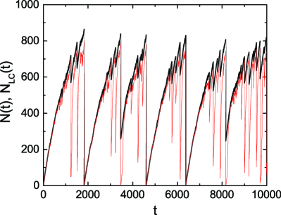
Figure 1: (Color online) Time dependences of the number of nodes $N(t)$ in the network $\mathcal{G}(t)$ (thick black line) and number of nodes $N_{\text{LC}}(t)$ in its largest component (thin red line). The node tolerance parameter is set as $m=5.0$.

III.1 Number of nodes and other network measures

We first examine the time dependence of the size of the network $\mathcal{G}(t)$. Figure 1 shows the number of nodes $N(t)$ in $\mathcal{G}(t)$ for the first $10^{4}$ time steps. The result clearly demonstrates that the network cannot grow infinitely and the size $N(t)$ largely fluctuates by repetitive growth and decay of the network. We can find some features in the line shape of $N(t)$. In the early stage, $N(t)$ increases almost monotonically with time, because the probability that any of the nodes in the network fail is low due to small $N_{0}(t)\,[=N(t-1)+1]$. Namely, in this time region, the expectation number of failed nodes is less than $1$. After this region, the expectation value becomes larger than $1$ and some nodes fail in $\mathcal{G}_{0}(t)$. However, since $r[N_{0}(t)]$ for still small $N_{0}(t)$ is rather large, cascades are not widely spread. Thus, $N(t)$ for $400\lesssim t\lesssim 800$ keeps increasing with relatively small drops. When $N(t)$ becomes larger than $800$, $r[N_{0}(t)]$ is so small that a cascade of failures never stops until all nodes are eliminated. Such complete collapses occur at $t=1,824$, $4,603$, and $6,374$ in Fig. 1. After a complete collapse, the system evolves in a similar manner to the evolution from $t=0$. In addition to $N(t)$, we plot in Fig. 1 the size of the largest component $N_{\text{LC}}(t)$ contained in $\mathcal{G}(t)$. The size $N_{\text{LC}}(t)$ basically follows the variation of $N(t)$ at most of the time steps, but sometimes $N_{\text{LC}}(t)$ drops substantially though $N(t)$ does not change so much. At these times, the network is decomposed into small components by cascading overload failures. The statistics of magnitudes of drops in $N(t)$, i.e., cascade sizes, will be argued in the next subsection.

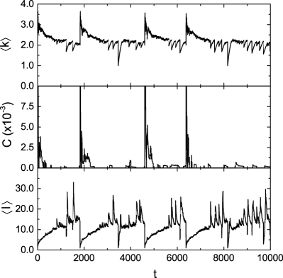
Figure 2: Time dependences of the average degree (top), the clustering coefficient (middle), and the average path length (bottom) of the network $\mathcal{G}(t)$. The node tolerance parameter is set as $m=5.0$. These quantities for the largest component of $\mathcal{G}(t)$ are not shown in this figure, because their line shapes almost overlap with those for $\mathcal{G}(t)$.

We also calculated several quantities that characterize the network structure at time $t$. Figure 2 shows the average degree $\langle k\rangle$, the clustering coefficient $C$, and the average path length $\langle l\rangle$ of the network $\mathcal{G}(t)$ as a function of $t$. These quantities for the largest component of $\mathcal{G}(t)$ take almost the same values as those for $\mathcal{G}(t)$. The average degree fluctuates around $\langle k\rangle=2(=\mu)$ though it becomes significantly larger than this value immediately after a complete collapse. We have confirmed that the degree distribution $\mathcal{P}(k)$ of $\mathcal{G}(t)$ hardly depends on time and decays exponentially for large $k$ if $N(t)$ is large enough (not shown here). This is reasonable because random attachment of new nodes and cascading failures without introducing degree correlations make the network topology similar to a homogeneous random graph. The clustering coefficient $C$ is quite small ($C\lesssim 10^{-4}$), except for $\mathcal{G}(t)$ at and just after complete collapses. At a complete collapse, $C$ is equal to $1$ because $\mathcal{G}(t)$ is a triangular ring at this time. The clustering coefficient, however, rapidly decreases with the network growth by random attachments. Sometimes $C$ becomes equal to zero, which implies that the network takes a tree (or forest) structure. The average path length $\langle l\rangle$ of the network at a complete collapse is obviously $1$, and after that $\langle l\rangle$ increases gradually with relatively large fluctuations. Considering that $N(t)$ is less than $1,000$, $\langle l\rangle$ close to or more than $10$ is too large to regard the network as being small world. Then, we can expect that $\mathcal{G}(t)$ giving very large $\langle l\rangle$ has a fractal structure. Before discussing the fractality of generated networks, it will be examined in the next subsection whether our dynamical system exhibits SOC behavior.

III.2 Avalanche size and self-organized criticality

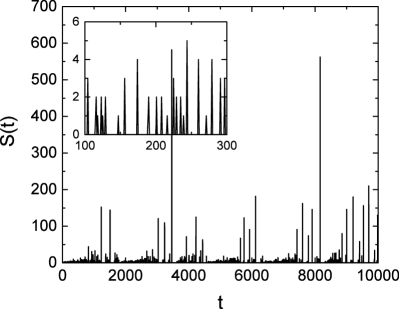
Figure 3: Time dependence of the avalanche size $S(t)$ obtained from $N(t)$ shown in Fig. 1. To make the figure easy to see, cascades leading to complete collapses are eliminated from the figure. The intermittency of cascades is found in the inset that magnifies the main figure for $100\leq t\leq 300$.

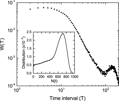
Figure 4: Distribution function $W(T)$ of the inactive time interval $T$ during which no overload failure occurs. The distribution $W(T)$ is obtained from the dynamics up to $t=5\times 10^{6}$ under the condition $m=5.0$. The inset shows the distribution of $N(t)$ in the same dynamics.

Sudden drops of the network size $N(t)$ found in Fig. 1 corresponds to decays of the network by cascading overload failures. Magnitudes of these drops represent scales of cascading overload failures. Here we define the avalanche size $S(t)$ as the number of nodes that are removed during a single cascade of overload failures occurring at the time $t$. Figure 3 shows the avalanche size $S(t)$ obtained from $N(t)$ shown in Fig. 1. The avalanche size largely fluctuates even if one ignores huge $S(t)$’s at complete collapses. Values of $S(t)$ at most of the time steps are less than $50$, while on rare occasions $S(t)$ exceeds $300$. The inset of Fig. 3 demonstrates that these avalanches occur intermittently with inactive intervals. This intermittency suggests a possibility that the network dynamics possesses SOC characteristics. In order to find further evidences of SOC dynamics, we examine the distribution function $W(T)$ of the inactive time interval $T$ between avalanches. The distribution $W(T)$ obtained from the dynamics under the same conditions as those for Fig. 1 but continued up to $5\times 10^{6}$ time steps is presented in Fig. 4. This figure clearly shows that $W(T)$ obeys a power law,

$$W(T)\propto T^{-\eta},$$ (11)

in an intermediate region of $T$. The least-squares fit for the data within $20\leq T\leq 50$ gives $\eta=3.00\pm 0.03$. The small hump near $T\sim 150$ comes from a finite-size effect related to the existence of the most probable network size $N_{\text{typ}}$. This size is about $700$ for our choice of the model parameters as depicted in the inset of Fig. 4. We have confirmed the correlations between $N(t)$ and $S(t)$ and between the inactive interval $T$ after a cascade and the cascade (avalanche) size $S$. These correlations and $N_{\text{typ}}\sim 700$ lead the frequently-appearing time interval at $T\sim 150$.

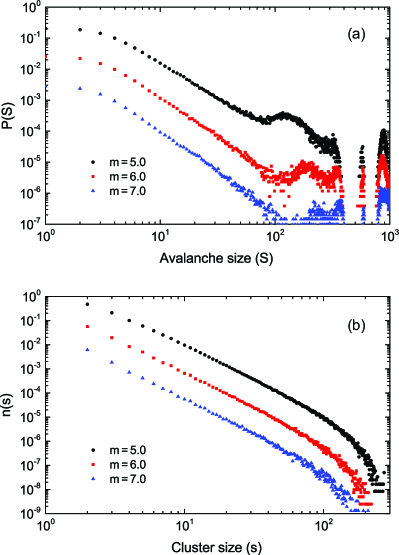
Figure 5: (Color online) (a) Distribution function $P(S)$ of the avalanche size $S$ and (b) the distribution function $n(s)$ of the cluster size $s$ for different values of the node tolerance parameter, i.e., $m=5.0$, $6.0$, and $7.0$. The distributions $P(S)$ and $n(s)$ are obtained from the dynamics up to $t=5\times 10^{6}$. In both panels, the distributions for $m=6.0$ and $7.0$ are vertically shifted for clarity.

The distributions of the avalanche size $S$ for several values of the node tolerance parameter $m$ are presented in Fig. 5(a). The avalanche size distribution $P(S)$ also follows a power-law relation, i.e.,

$$P(S)\propto S^{-\lambda}.$$ (12)

Our result indicates that the exponent $\lambda$ does not depend on $m$ and is estimated as $\lambda=2.60\pm 0.02$ for $m=7.0$. The rightmost hump in $P(S)$ at around $S\sim 900$ represents the contribution from complete collapses. The second hump from the right corresponds to decays of large networks to assemblies of dimers. Moreover, the broad hump near $S=150$ found in the result for $m=5.0$ is related to the hump in $W(T)$ shown by Fig. 4. This broad hump represents the typical avalanche size of cascades from typical networks with $N_{\text{typ}}\sim 700$ nodes. Therefore, these humps are attributable to finite-size effects associated with our choice of the model parameters.

Figure 5(b) shows the cluster size distribution $n(s)$ for three different values of $m$. The cluster size $s$ at time $t$ is the number of nodes in a component included in the network $\mathcal{G}(t)$. The cluster size distribution function $n(s)$ is calculated from all components of the network at every time step in the entire dynamics. The distribution $n(s)$ has a power-law form,

$$n(s)\propto s^{-\tau},$$ (13)

as well as $W(T)$ and $P(S)$. The exponent $\tau$, calculated as $\tau=2.92\pm 0.02$ for $m=7.0$, is also independent of $m$. In contrast to the distribution $P(S)$, the influence of complete collapses to $n(s)$ is inconspicuous. This is because the size of a network just after a complete collapse is $N_{\text{ini}}(=3)$ and the number of components with $s=3$ generated in the whole period of the network evolution is extremely large compared to the number of complete collapses occurring in the same period.

All the above results, namely the intermittency of $S(t)$ and the power-law forms of $W(T)$, $P(S)$, and $n(s)$, strongly support that the dynamics of network structure in our model exhibits SOC behavior. These results also show that the universality class of self-organized criticality does not depend on the node tolerance parameter $m$. The relation to other parameters will be discussed later.

III.3 Fractal and small-world networks

As we mentioned in Sect. II.1, a cascade of overload failures gives a fatal damage to a connected network $\mathcal{G}_{0}$ of size $N_{0}$ if the load reduction parameter $r$ is less than $r_{\text{c}}(N_{0})$, and the giant component after a cascade at $r=r_{\text{c}}(N_{0})$ has a fractal structure Mizutaka15 . In the present SOC model, on the other hand, $r$ decreases with the network size $N_{0}(t)$. For $r[N_{0}(t)]$ chosen as Eq. (10), the parameter $r$ decreases from a large enough value $r_{\text{max}}$ for $N_{0}(t)\leq N_{\text{ini}}$ to zero for $N_{0}(t)\geq N_{\text{max}}$. Since any network is completely collapsed by a cascade of failures at $r=0$, through the network growth, $r[N_{0}(t)]$ must eventually encounter the critical value $r_{\text{c}}$ at which the cascade of failures provides the percolation transition of the network. (Precisely speaking, the term “critical” is not appropriate because $N_{0}(t)$ is finite. However, we use this terminology by supposing the case that sufficiently large networks are generated under suitable values of the model parameters. The word “critical” in the rest of this paper will be used in the same sense.) If a network with the size $N_{0}(t)$ satisfying $r[N_{0}(t)]=r_{\text{c}}$ experiences a cascade of overload failures, we expect that the giant component after the cascade has a fractal structure.

In the case of cascading failures starting with a fixed connected network $\mathcal{G}_{0}$ of size $N_{0}$ in which all the capacities of nodes are definitely determined by their degrees and the initial total load $W_{0}$, the value of $r_{\text{c}}(N_{0})$ is theoretically calculated as addressed in the last paragraph of Sect. II.1 Mizutaka15 . In our SOC model, however, the capacity of a node depends on the total load at the time when the node was introduced in the system. Thus, the node capacities in the network $\mathcal{G}_{0}(t)$ depends strongly on the past history of $\mathcal{G}_{0}(t)$, and the critical load reduction parameter $r_{\text{c}}$ cannot be uniquely determined by the size of $\mathcal{G}_{0}(t)$. Since the theoretical method proposed by Ref. References is not applicable to dynamics governed by such hysteresis effects, we need to examine numerically whether $r[N_{0}(t)]$ of the network $\mathcal{G}_{0}(t)$ is close to an unknown value of $r_{\text{c}}$ peculiar to $\mathcal{G}_{0}(t)$.

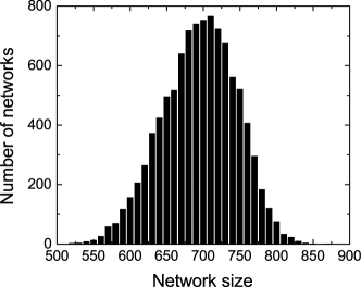
Figure 6: Histogram of the number of pre-critical networks just before critical cascades versus the size of the pre-critical network. The histogram is obtained for the first $10^{4}$ critical cascades occurring in the dynamics under the condition $m=5.0$.

If $r[N_{0}(t)]$ of the network $\mathcal{G}_{0}(t)$ is much larger than $r_{\text{c}}$, a cascade of overload failures, if any, eliminates only a small fraction of nodes from $\mathcal{G}_{0}(t)$ and does not change the giant component size so much. On the other hand, a cascade with $r[N_{0}(t)]\ll r_{\text{c}}$ causes a complete collapse of $\mathcal{G}_{0}(t)$. If $r[N_{0}(t)]$ is close to $r_{\text{c}}$, the cascade is marginal, for which the size of the giant component after the cascade must be much smaller than the original giant component size of $\mathcal{G}_{0}(t)$ but still much larger than $N_{\text{ini}}$. From the above consideration, we regard in this work a cascade of overload failures at time $t$ satisfying the following conditions as a critical cascade whose load reduction parameter should be close to $r_{\text{c}}$:

$$\frac{N_{\text{LC}}(t)}{N_{\text{LC}}(t-1)}\leq 0.5\quad\text{and}\quad N_{\text{LC}}(t)\geq 100,$$ (14)

where $N_{\text{LC}}(t)$ is the number of nodes in the largest component of $\mathcal{G}(t)$. The specific values $0.5$ and $100$ in Eq. (14) are not important as long as $N_{\text{LC}}(t)/N_{\text{LC}}(t-1)$ and $N_{\text{LC}}(t)$ are much smaller and larger than $1$, respectively. In the sense of the percolation transition by cascading overload failures, a network after completing a critical cascade can be considered as a critical network $\mathcal{G}_{\text{c}}$. Also, we call a network just before a critical cascade a pre-critical network $\mathcal{G}_{\text{pre}}$. Figure 6 shows the histogram of the number of pre-critical networks as a function of the size of $\mathcal{G}_{\text{pre}}$. This result indicates that critical cascades are likely to occur on networks of size $N(t)\sim 700$ for the present parameter set. Considering that the most probable network size $N_{\text{typ}}$ is also about $700$ as shown by the inset of Fig. 4, critical cascades take place frequently during SOC dynamics. This means that critical networks are generated very often by such cascades.

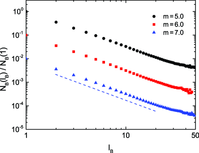
Figure 7: (Color online) $N_{\text{B}}(l_{\text{B}})$ for giant components in critical networks generated by SOC dynamics under the conditions $m=5.0$, $6.0$, and $7.0$. The longitudinal axis indicates $N_{\text{B}}(l_{\text{B}})/N_{\text{B}}(1)$ averaged over $1,000$ realizations of critical networks. The results for $m=6.0$ and $7.0$ are vertically shifted for clarity. The straight dashed line has the slope $d_{\text{B}}=1.53$ which is obtained by the least-squares fit for the data for $m=7.0$ from $l_{\text{B}}=2$ to $20$.

We study the fractal property of giant components in critical networks. As we explained in Sect. I, if a given connected network is fractal, the minimum number $N_{\text{B}}(l_{\text{B}})$ of subgraphs of diameter less than $l_{\text{B}}$ required to cover the network satisfies the relation

$$N_{\text{B}}(l_{\text{B}})\propto l_{\text{B}}^{-d_{\text{B}}},$$ (15)

where $d_{\text{B}}$ is the fractal dimension of the network Song05 . We calculate $N_{\text{B}}(l_{\text{B}})$ for giant components in $1,000$ critical networks appearing in the dynamics by using the compact-box-burning algorithm Song07 and average $N_{\text{B}}(l_{\text{B}})/N_{\text{B}}(1)$ over these realizations, where $N_{\text{B}}(1)$ is equal to the number of nodes in the largest component. The results for $m=5.0$, $6.0$, and $7.0$ are plotted in Fig. 7. These plots clearly demonstrate that the quantity $N_{\text{B}}(l_{\text{B}})$ satisfies Eq. (15) and the fractal dimension $d_{\text{B}}$ does not depend on $m$. The value of $d_{\text{B}}$ estimated from the result for $m=7.0$ is $1.53\pm 0.01$. It is interesting that this fractal dimension is close to $d_{\text{B}}=1.54\pm 0.01$ that has been computed for the giant component after a critical cascade starting with an Erdős-Rényi (ER) random graph Mizutaka15 . The topology of a pre-critical network $\mathcal{G}_{\text{pre}}$ in SOC dynamics is not the same as that of the ER random graph $\mathcal{G}_{\text{ER}}$. In addition, the capacity of a node in $\mathcal{G}_{\text{pre}}$ depends on the total load of the system when the node was introduced, while the node capacity in $\mathcal{G}_{\text{ER}}$ is determined by the degree of the node and a fixed initial total load $W_{0}$. In spite of these discrepancies, it is not surprising that both fractal dimensions are the same, which implies the same universality class between percolation transitions for $\mathcal{G}_{\text{pre}}$ and $\mathcal{G}_{\text{ER}}$. This is because the degree distribution of $\mathcal{G}_{\text{pre}}$ has an exponential tail, like that of $\mathcal{G}_{\text{ER}}$, and the node capacity distribution is not wide, which behaves similarly to the distribution of $N(t)$ shown in the inset of Fig. 4.

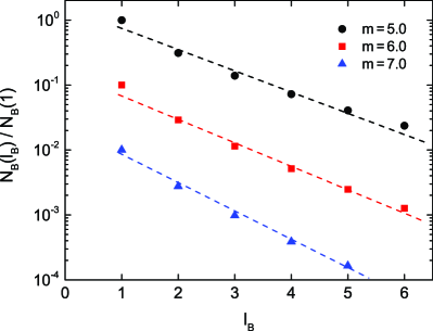
Figure 8: (Color online) $N_{\text{B}}(l_{\text{B}})$ for largest components in networks that first reach the size $N(t)=300$ after complete collapses in SOC dynamics under the conditions $m=5.0$, $6.0$, and $7.0$. The longitudinal axis indicates $N_{\text{B}}(l_{\text{B}})/N_{\text{B}}(1)$ averaged over $1,000$ realizations of such networks. The results for $m=6.0$ and $7.0$ are vertically shifted for clarity. The dashed lines are guides to the eye.

Let us examine $N_{\text{B}}(l_{\text{B}})$ for off-critical networks. If a network is far from criticality, we can expect that the network has a small-world structure, because the network formed by random attachment of new nodes has many short-cut edges. For a small-world network, the number of covering subgraphs $N_{\text{B}}(l_{\text{B}})$ decreases exponentially with $l_{\text{B}}$, namely,

$$N_{\text{B}}(l_{\text{B}})\propto\exp(-l_{\text{B}}/l_{0}),$$ (16)

where $l_{0}$ is a characteristic path length. We calculated $N_{\text{B}}(l_{\text{B}})$ for networks (or their largest components if not connected) that first reach the size $N(t)=300$ after complete collapses, and averaged $N_{\text{B}}(l_{\text{B}})/N_{\text{B}}(1)$ over $1,000$ realizations of such networks in SOC dynamics. The results shown in Fig. 8 indicate the small-world property of these networks. Our SOC model thus generates both fractal and small-world networks in a single dynamics.

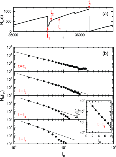
Figure 9: (Color online) (a) Time dependence of the number of nodes $N_{\text{LC}}(t)$ in the largest component of the network $\mathcal{G}(t)$ in the dynamics for $m=7.0$. The arrows indicate the times at which $N_{\text{B}}(l_{\text{B}})$’s are calculated. (b) $N_{\text{B}}(l_{\text{B}})$’s for largest components in $\mathcal{G}(t_{1})$, $\mathcal{G}(t_{2})$, $\mathcal{G}(t_{3})$, and $\mathcal{G}(t_{4})$ from top to bottom. Thin lines are guides to the eye. The rapid decrease of $N_{\text{B}}(l_{\text{B}})$ for $l_{\text{B}}\gg l_{\text{co}}$ at $t=t_{3}$ or $t_{4}$ indicates that the largest component has a small-world structure in a longer length-scale than $l_{\text{co}}$. The inset shows $N_{\text{B}}(l_{\text{B}})$ at $t=t_{4}$ in a semi-logarithmic scale.

We further investigate the crossover behavior from fractal to small-world structure associated with the time evolution from a critical network. Figure 9 illustrates a typical profile change of $N_{\text{B}}(l_{\text{B}})$ for networks formed at several times from $t_{1}$ at which a critical network appears to $t_{4}$ just before the next complete collapse. The times at which $N_{\text{B}}(l_{\text{B}})$’s are calculated are indicated in Fig. 9(a) by arrows on the time dependence of the largest component size $N_{\text{LC}}(t)$. At $t=t_{1}$, $N_{\text{B}}(l_{\text{B}})$ follows a power law, which suggests that the giant component in $\mathcal{G}(t_{1})$ has a fractal structure as we expect. After this time, the largest component size rapidly increases as shown in Fig. 9(a). This is because newly added nodes are more likely to merge separated fractal components but less likely to be connected onto a single component. Therefore, the largest component at $t=t_{2}$ remains fractal at almost any scale. When the time elapses further, the increase of $N_{\text{LC}}(t)$ becomes moderate. This implies that the merging process of separated components has been mostly finished and new nodes are simply incorporated in the largest component. In this case, newly added nodes bring short-cut edges in the largest component, which makes the network small-world as shown by $N_{\text{B}}(l_{\text{B}})$ at $t=t_{3}$ in Fig. 9(b). More precisely, the network is small-world in a longer length scale than the average distance $l_{\text{co}}$ between terminal nodes of short-cut edges introduced by new nodes, while it is fractal for $l_{\text{B}}\ll l_{\text{co}}$. This situation is similar to the case that a lattice-like network changes into a small-world one by random rewirings in the Watts-Strogatz model Barthelemy99 In fact, a high density of short-cut edges at $t=t_{4}$ reduces the crossover length $l_{\text{co}}$ and the small-world property can be found in the whole $l_{\text{B}}$ range as shown by the inset of Fig. 9(b).

III.4 Suitable choice of parameter values

All the above arguments are based on specific values of the model parameters. If the dynamical properties presented above are peculiar to these parameter values, it cannot be said that the present model exhibits self-organized criticality, because of the necessity of tuning the external parameters. It has, however, been confirmed that the results are essentially independent of the choice of parameter values if these parameters lie in suitable ranges. In this subsection, we discuss the suitable parameter ranges to realize SOC dynamics.

To find the suitable ranges of parameter values, let us consider how large a network could grow if the system did not experience any critical cascades and complete collapses. Even in this case, a network cannot grow infinitely. The expectation number $\langle S\rangle$ of eliminated nodes per unit time step increases with the network size $N(t)$, and eventually $\langle S\rangle$ reaches the incrementation of $N(t)$ at every time step due to the participation of a new node. Once this is the case, the network does not grow any more. The network size $N(t)$ then fluctuates around a stationary size with small amplitudes. The stationary size $N_{\text{st}}$ can be roughly estimated by the overload probability. In the absence of critical cascades and complete collapses, we can consider approximately that all cascading overload failures stop at the first step of the cascade process and subsequent avalanches triggered by the first failures do not occur, because avalanche sizes are small. This approximation enables us to calculate the steady-state expectation number of failed nodes per unit time step by

$$\langle S\rangle=N_{\text{st}}\sum_{k}\mathcal{P}_{\text{st}}(k)F_{W(N_{\text{st}})}(k),$$ (17)

where $\mathcal{P}_{\text{st}}(k)$ is the degree distribution of a steady-state network $\mathcal{G}_{\text{st}}$ and $F_{W(N_{\text{st}})}(k)$ is the overload probability of a node of degree $k$ in $\mathcal{G}_{\text{st}}$. With the aid of the regularized incomplete beta function, the probability $F_{W(N_{\text{st}})}(k)$ is, with reference to Eq. (3), given by

$$F_{W(N_{\text{st}})}(k)=I_{k/\mu N_{\text{st}}}\left[\lfloor q_{\mu}(N_{\text{st}})\rfloor+1,W(N_{\text{st}})-\lfloor q_{\mu}(N_{\text{st}})\rfloor\right],$$ (18)

where

$$q_{\mu}(N_{\text{st}})=\frac{a\mu}{2}+m\sqrt{\frac{a\mu}{2}\left(1-\frac{1}{N_{\text{st}}}\right)},$$ (19)

and

$$W(N_{\text{st}})=\frac{a\mu N_{\text{st}}}{2}.$$ (20)

Here, we approximated the average degree of $\mathcal{G}_{\text{st}}$ by $\mu$ for the reason that nodes with degree greater than $\mu$ are more likely to be eliminated by overload failures in $\mathcal{G}_{\text{st}}$ while the average degree would be larger than $\mu$ (equal to $2\mu$) if the network monotonically grew without any node elimination. In the steady state, $\langle S\rangle$ must be equal to the incrementation of the network size per unit time step, namely $1$. Therefore, the stationary size $N_{\text{st}}$ is determined by the relation,

$$N_{\text{st}}=\frac{1}{\sum_{k}\mathcal{P}_{\text{st}}(k)F_{W(N_{\text{st}})}(k)}.$$ (21)

If we neglect critical cascades and complete collapses, the network can grow up to the size $N_{\text{st}}$ obtained by solving the above transcendental equation. But actually, the network encounters critical cascades or complete collapses before reaching this size if $N_{\text{st}}$ is larger than the typical size $N_{\text{pre}}$ of pre-critical networks $\mathcal{G}_{\text{pre}}$. In this case, and only in this case, critical cascades generate fractal networks, and the present model exhibits SOC character. Otherwise, critical cascades themselves never take place in the dynamics. Thus, the condition to realize SOC dynamics is

$$N_{\text{st}}\gg N_{\text{pre}}\gg 1,$$ (22)

where the condition $N_{\text{pre}}\gg 1$ guarantees that the system is large enough to exhibit genuine self-organized criticality. What is the relation between the above condition and the model parameters? Among several parameters characterizing our model, parameters related to the initial network $\mathcal{G}(0)$, namely, $N_{\text{ini}}$, $M_{\text{ini}}$, and the topology of $\mathcal{G}(0)$, are obviously irrelevant to the condition (22). It is thus significant to elucidate how $N_{\text{st}}$ and $N_{\text{pre}}$ depend on $a$ (the load carried by a single edge), $m$ (the node tolerance parameter), $\mu$ (the number of edges of a newly added node), and the functional form of the load reduction parameter $r(N)$.

The stationary size $N_{\text{st}}$ depends on $a$, $m$, and $\mu$. Equation (21) reveals the relation of $N_{\text{st}}$ to these parameters. Since the preferential elimination of nodes with degree much larger than $\mu$ in $\mathcal{G}_{\text{st}}$ gives a sharp peak of $\mathcal{P}_{\text{st}}(k)$ at $k=\mu$, $\mathcal{P}_{\text{st}}(k)$ hardly depends on $N_{\text{st}}$. Furthermore, the overload probability $F_{W(N_{\text{st}})}(k)$ presented by Eq. (18) indeed depends only very weakly on $N_{\text{st}}$, which comes from the property of the regularized incomplete beta function. Therefore, Eq. (21) is not actually transcendental, and $N_{\text{st}}$ can be evaluated by $\mathcal{P}_{\text{st}}(k)$ and $F_{W(N)}(k)$ for a haphazardly chosen value of $N(\gg\mu)$. The probability $F_{W(N)}(k)$ given by Eqs. (18)-(20) with $N_{\text{st}}$ replaced by $N$ is a decreasing function of $m$ and $\mu$ for any $k$. Hence, $N_{\text{st}}$ obtained by Eq. (21) increases with $m$ and $\mu$ regardless of $\mathcal{P}_{\text{st}}(k)$. The $a$ dependence of $F_{W(N)}(k)$ is, however, influenced by the value of $k$. $F_{W(N)}(k)$ increases with $a$ if $k>\mu$, while it decreases for $k<\mu$. Meanwhile, for a fixed value of $a$, $F_{W(N)}(k)$ for $k<\mu$ is negligibly small. Thus, $F_{W(N)}(k)$ for $k$ larger than $\mu$ dominates the summation in Eq. (21), independently of the form of $\mathcal{P}_{\text{st}}(k)$. This fact and the property of $F_{W(N)}(k)$ of being an increasing function of $a$ for $k>\mu$ show that $N_{\text{st}}$ decreases with $a$. Consequently, we need to choose large values of $m$ and $\mu$ and a small value of $a$ to obtain large $N_{\text{st}}$.

On the other hand, $N_{\text{pre}}$ is the typical size of a network whose load reduction parameter $r$ is equal to the critical value $r_{\text{c}}$ specific to the network. The parameter $r$ is uniquely determined by the network size $N$, while $r_{\text{c}}$ depends not only on $N$ but also on the past history of the network. Approximating the typical size of pre-critical networks by the size of a typical pre-critical network $\mathcal{G}_{\text{pre}}$, $N_{\text{pre}}$ must satisfy

$$r(N_{\text{pre}})=r_{\text{c}}[\mathcal{G}_{\text{pre}}(N_{\text{pre}})],$$ (23)

where $r_{\text{c}}[\mathcal{G}_{\text{pre}}(N_{\text{pre}})]$ is the critical load reduction parameter of $\mathcal{G}_{\text{pre}}$ whose size is $N_{\text{pre}}$. Since the right-hand size of Eq. (23) is a function of $a$, $m$, $\mu$, and $N_{\text{pre}}$, the size $N_{\text{pre}}$ as the solution of Eq. (23) depends on these parameters in addition to the functional form of $r(N)$. If $r(N)$ decreases slowly with $N$, however, the solution $N_{\text{pre}}$ is mainly governed by the form of $r(N)$ rather than the precise value of $r_{\text{c}}$. In order to satisfy $N_{\text{pre}}\gg 1$, $r(N)$ needs to decrease very slowly with the network size. In the case that $r(N)$ is set as Eq. (10), $N_{\text{max}}$ must be chosen to be large enough.

In conclusion, the load reduction parameter $r(N)$ must decrease with $N$ very slowly to realize the condition $N_{\text{pre}}\gg 1$, and the node tolerance parameter $m$ and the load by edge $a$ should be large and small enough, respectively, so that $N_{\text{st}}$ becomes much larger than $N_{\text{pre}}$. Although a large value of $\mu$ is preferable for the condition $N_{\text{st}}\gg N_{\text{pre}}$, results are not strongly influenced by $\mu$ because the number of edges of a new node is always restricted by $2\leq\mu\leq N_{\text{ini}}$ with small $N_{\text{ini}}$. Our choice of values for $a$, $m$, and $\mu$ in this section obviously satisfies the condition $N_{\text{st}}\gg N_{\text{pre}}$, because we have critical cascades in the dynamics. In fact, $N_{\text{st}}$ estimated by Eq. (21) with the numerically obtained $\mathcal{P}_{\text{st}}(k)$ is $861$ for $a=2.0$, $\mu=2$, and $m=5.0$, which is larger than $N_{\text{pre}}\simeq 700$ as indicated in Fig 6. We have confirmed that the universality class of self-organized criticality, namely the set of the exponents $\eta$, $\lambda$, $\tau$, and $d_{\text{B}}$, does not depend on the choice of parameter values if the condition (22) is satisfied. It has also been checked that the functional form of $r(N)$ is irrelevant to SOC dynamics as far as $r(N)$ is a slowly decreasing function of $N$.

IV Summary

We have proposed a model of self-organized critical (SOC) dynamics of complex networks and presented a possible explanation of the emergence of fractal and small-world networks. Our model combines a network growth and its decay due to the instability of large grown networks against cascading overload failures. Cascading failures occur intermittently and prevent networks from growing infinitely. The distribution of the inactive time interval between successive cascades of failures has a power-law form. Both the avalanche size that is the number of eliminated nodes in a single cascade and the cluster size defined as the number of nodes in a connected component also obey power-law distributions. These facts indicate that the network dynamics possesses SOC characteristics. During the SOC dynamics, the load reduction parameter $r$ varies with the network size. When $r$ of the network coincides with its critical value $r_{\text{c}}$, a cascade of overload failures (critical cascade) decays the network into a critical one. We have shown that giant components just after critical cascades have fractal structures. The fractal dimension $d_{\text{B}}$ is close to that for the giant component after a critical cascade starting with an Erdős-Rényi random graph. In contrast, networks far from criticality display the small-world property. In particular, we demonstrated the crossover behavior from fractal to small-world structure in a growing process from a critical network, which is caused by short-cut edges introduced by newly added nodes. We have also discussed suitable parameter values to realize SOC dynamics.

It is significant to notice that the present model is somewhat different from previous SOC models. In a conventional SOC model, a routine procedure in the dynamics, such as placement of grains of sand in the sandpile model Bak87 or renewals of fitness values in the Bak-Sneppen model Bak93 , takes a system close to the critical point, but the instability of critical or near-critical states drives the system away from criticality accompanied by some sort of avalanches. In our model, on the other hand, the network growth as a routine procedure takes the system away from the critical point, but the instability of large grown networks makes the network critical. Although the roles of growth and instability are opposite to those of conventional models, the system described by our model exhibits the most of SOC characteristics as explained in Sect. III. This implies that the present model provides a new type of self-organized criticality. Our model generates non-scale-free networks with homogeneous degree distributions and belongs to a specific universality class of SOC dynamics, independently of the choice of values of the model parameters. It is then interesting to study how the model should be modified to belong to another class of self-organized criticality with forming scale-free networks.

- (1) R. Albert and A.-L. Barabási, Rev. Mod. Phys. 74, 47 (2002).
- (2) S. N. Dorogovtsev and J. F. F. Mendes, Evolution of networks: From biological nets to the Internet and WWW (Oxford Univ. Press, Oxford, 2003).
- (3) R. Cohen and S. Havlin, Complex Networks: Structure, Robustness and Function (Cambridge Univ. Press, Cambridge, 2010).
- (4) A.-L. Barábasi and R. Albert, Science 286, 509 (1999).
- (5) M. E. J. Newman, Phys. Rev. Lett. 89, 208701 (2002).
- (6) M. E. J. Newman, Phys. Rev. E 67, 026126 (2003).
- (7) M. Girvan and M. E. J. Newman, Proc. Natl. Acad. Sci. USA 99, 7821 (2002).
- (8) D. J. Watts and S. H. Strogatz, Nature 393, 440 (1998).
- (9) C. Song, S. Havlin, and H. A. Makse, Nature 433, 392 (2005).
- (10) J. M. Montoya and R. V. Solé, J. Theor. Biol. 214, 405 (2002).
- (11) L. A. N. Amaral, A. Scala, M. Barthélémy, and H. E. Stanley, Proc. Natl. Acad. Sci. USA 97, 11149 (2000).
- (12) D. S. Bassett and E. T. Bullmore, Neuroscientist 12, 512 (2006).
- (13) M. D. Humphries and K. Gurney, PLoS ONE 3, e0002051 (2008).
- (14) F. Kawasaki and K. Yakubo, Phys. Rev. E 82, 036113 (2010).
- (15) G. Csányi and B. Szendröi, Phys. Rev. E 70, 016122 (2004).
- (16) G. Concas, M. F. Locci, M. Marchesi, S. Pinna, and I. Turnu, Europhys. Lett. 76, 1221 (2006).
- (17) C. R. Myers, Phys. Rev. E 68, 046116 (2003).
- (18) R. Cohen and S. Havlin, Physica A 336, 6 (2004).
- (19) K.-I. Goh, G. Salvi, B. Kahng, and D. Kim, Phys. Rev. Lett. 96, 018701 (2006).
- (20) C. Song, S. Havlin, and H. A. Makse, Nat. Phys. 2, 275 (2006).
- (21) H. D. Rozenfeld, S. Havlin, and D. ben-Avraham, New J. Phys. 9, 175 (2007).
- (22) C. Song, L. K. Gallos, S. Havlin, and H. A. Makse, J. Stat. Mech. 2007, P03006 (2007).
- (23) S. Furuya and K. Yakubo, Phys. Rev. E 84, 036118 (2011).
- (24) Y. Sun and Y. Zhao, Phys. Rev. E 89, 042809 (2014).
- (25) P. Bak, C. Tang, and K. Wiesenfeld, Phys. Rev. Lett. 59, 381 (1987).
- (26) P. Bak and K. Sneppen, Phys. Rev. Lett. 71, 4083 (1993); M. Paczuski, S. Maslov, and P. Bak, Phys. Rev. E 53, 414 (1996).
- (27) D. Marković and C. Gros, Phys. Rep. 536, 41 (2014).
- (28) B. Drossel and F. Schwabl, Phys. Rev. Lett. 69, 1629 (1992).
- (29) H. Takayasu and H. Inaoka, Phys. Rev. Lett. 68, 966 (1992).
- (30) A. Rinaldo, I. Rodriguez-Iturbe, R. Rigon, E. Ijjasz-Vasquez, and R. L. Bras, Phys. Rev. Lett. 70, 822 (1993).
- (31) B. Sapoval, A. Baldassarri, and A. Gabrielli, Phys. Rev. Lett. 93, 098501 (2004).
- (32) L. de Arcangelis and H. J. Herrmann, Physica A 308, 545 (2002).
- (33) Y. Moreno and A. Vazquez, Europhys. Lett. 57, 765 (2002).
- (34) K.-I. Goh, D.-S. Lee, B. Kahng, and D. Kim, Phys. Rev. Lett. 91, 148701 (2003).
- (35) N. Masuda, K.-I. Goh, and B. Kahng, Phys. Rev. E 72, 066106 (2005).
- (36) M. Lin and T. L. Chen, Phys. Rev. E 71, 016133 (2005).
- (37) G. L. Pellegrini, L. de Arcangelis, H. J. Herrmann, and C. Perrone-Capano, Phys. Rev. E 76, 016107 (2007).
- (38) B. Luque, O. Miramontes, and L. Lacasa, Phys. Rev. Lett. 101, 158702 (2008).
- (39) H. Bhaumik and S. B. Santra, Phys. Rev. E 88, 062817 (2013).
- (40) A. Watanabe and K. Yakubo, Phys. Rev. E 89, 052806 (2014).
- (41) P.-A. Noël, C. D. Brummitt, and R. M. D’Souza, Phys. Rev. E 89, 012807 (2014).
- (42) T. Gross and B. Blasius, J. R. Soc. Interface 5, 259 (2008).
- (43) T. Aoki and T. Aoyagi, Phys. Rev. Lett. 109, 208702 (2012).
- (44) T. Shimada, Sci. Rep. 4, 4082 (2014).
- (45) K. Christensen, R. Donangelo, B. Koiller, and K. Sneppen, Phys. Rev. Lett. 81, 2380 (1998).
- (46) F. Slanina and M. Kotrla, Phys. Rev. Lett. 83, 5587 (1999).
- (47) D. Garlaschelli, A. Capocci, and G. Caldarelli, Nat. Phys. 3, 813 (2007).
- (48) C. Guill and B. Drossel, J. Theor. Bio. 251, 108 (2008).
- (49) T. P. Peixoto and C. P. C. Prado, Phys. Rev. E 69, 025101(R) (2004).
- (50) T. P. Peixoto and J. Davidsen, Phys. Rev. E 77, 066107 (2008).
- (51) P. Fronczak, A. Fronczak, and J. A. Hołyst, Phys. Rev. E 73, 046117 (2006).
- (52) D. Hughes, M. Paczuski, R. O. Dendy, P. Helander, and K. G. McClements, Phys. Rev. Lett. 90, 131101 (2003).
- (53) S. Bornholdt and T. Rohlf, Phys. Rev. Lett. 84, 6114 (2000).
- (54) M. Rybarsch and S. Bornholdt, PLoS ONE 9, e93090 (2014).
- (55) G. Bianconi and M. Marsili, Phys. Rev. E 70, 035105(R) (2004).
- (56) C.-W. Shin and S. Kim, Phys. Rev. E 74, 045101(R) (2006).
- (57) S. Mizutaka and K. Yakubo, Phys. Rev. E 92, 012814 (2015).
- (58) V. Kishore, M. S. Santhanam, and R. E. Amritkar, Phys. Rev. Lett. 106, 188701 (2011).
- (59) V. Kishore, M. S. Santhanam, and R. E. Amritkar, Phys. Rev. E. 85, 056120 (2012).
- (60) S. Mizutaka and K. Yakubo, Phys. Rev. E 88, 012803 (2013).
- (61) J. D. Noh and H. Rieger, Phys. Rev. Lett. 92, 118701 (2004).
- (62) M. Abramowitz and I. A. Stegun, Handbook of Mathematical Functions (Dover, New York, 1964).
- (63) M. E. J. Newman, S. H. Strogatz, and D. J. Watts, Phys. Rev. E 64, 026118 (2001).
- (64) M. Barthélémy and L. A. N. Amaral, Phys. Rev. Lett. 82, 3180 (1999).