Insights from Single-File Diffusion
into Cooperativity in Higher Dimensions

Abstract

Diffusion in colloidal suspensions can be very slow due to the cage effect, which confines each particle within a short radius on one hand, and involves large-scale cooperative motions on the other. In search of insight into this cooperativity, here the authors develop a formalism to calculate the displacement correlation in colloidal systems, mainly in the two-dimensional case. To clarify the idea for it, studies are reviewed on cooperativity among the particles in the one-dimensional case, i.e. the single-file diffusion (SFD). As an improvement over the celebrated formula by Alexander and Pincus on the mean-square displacement (MSD) in SFD, it is shown that the displacement correlation in SFD can be calculated from Lagrangian correlation of the particle interval in the one-dimensional case, and also that the formula can be extended to higher dimensions. The improved formula becomes exact for large systems. By combining the formula with a nonlinear theory for correlation, a correction to the asymptotic law for the MSD in SFD is obtained. In the two-dimensional case, the linear theory gives description of vortical cooperative motion.

Special Issue Comments: This article presents methodological insights into mathematical treatment of particle cooperativity in colloidal liquids. This article is related to the Special Issue articles [in Biophys. Rev. Lett.] about mathematical approaches to single-file diffusion[1] and Fourier-based analysis of quasi-one-dimensional systems[2].

Keywords: Single-file diffusion; Alexander–Pincus formula; cooperativity; collective motion; four-point correlations; displacement correlation; Brownian particles; dense colloidal suspensions; glassy systems; cage effect; elastic network; Lagrangian description of continuum mechanics; convected coordinate system

Electronic version of an article published as Biophys. Rev. Lett. 11, 9–38 (2016), DOI: 10.1142/S1793048015400019 © World Scientific Publishing Company http://www.worldscientific.com

1 Introduction

The slowdown of diffusion in systems of densely packed particles, as well as constrained dynamics in many other systems described as “glassy”, “jammed”, or “crowded”, has attracted attention[3], not only in connection with the physics of glass transition[4, 5] but also in the context of anomalous transport in biological cells[6]. The slowdown is due to suppression of free diffusion, which implies that the particles can diffuse only in some cooperative way with space-time correlations[7, 8].

For concreteness, we consider a colloidal system consisting of spherical Brownian particles in the ${n_{\text{d}}}$-dimensional space, with the representative diameter $\sigma$. We denote the position vector of the $i$-th particle with $\mathbf{r}_{i}(t)$; there are $N$ particles so that $i=1,2,\ldots,N$. The particles are governed by the Langevin equation,

$$m\ddot{\mathbf{r}}_{i}=-\mu\dot{\mathbf{r}}_{i}-\frac{\partial}{\partial\mathbf{r}_{i}}\sum_{j<k}V_{jk}+\mu\mathbf{f}_{i}(t),$$ (1.1)

where $m$ is the mass of the particle, $V_{jk}$ is the interaction potential between the $j$-th and $k$-th particles, and $\mu\mathbf{f}_{i}(t)$ is the random force characterized by the variance

$$\left\langle{\mathbf{f}_{i}(t)\otimes\mathbf{f}_{j}(t^{\prime})}\right\rangle=\frac{2{k_{\text{B}}}T}{\mu}\delta_{ij}\delta(t-t^{\prime})\openone.$$ (1.2)

The drag coefficient $\mu$, which may depend on the configuration of the particles in general, is regarded here as constant for simplicity. The system is assumed to fill a periodic box of the linear dimension $L$ and to be uniform statistically, unless specified otherwise, and we consider the thermodynamic limit, $L\to\infty$, keeping the mean density $\rho_{0}=N/L^{n_{\text{d}}}$ fixed.

To study slowdown of diffusion, let us start with denoting the displacement of the $j$-th particle with $\mathbf{R}_{j}(t,s)=\mathbf{r}_{j}(t)-\mathbf{r}_{j}(s)$, where $s<t$; if the system is statistically steady, it suffices to consider $\mathbf{R}_{j}(t)=\mathbf{r}_{j}(t)-\mathbf{r}_{j}(0)$. The mean-square displacement (MSD) is given by $\left\langle{\mathbf{R}^{2}}\right\rangle=\left\langle{[\mathbf{R}_{j}(t)]^{2}}\right\rangle$, with $\left\langle{~{}\cdot~{}}\right\rangle$ denoting the ensemble average in regard to the random force, as in Eq. (1.2), and the subscript $j$ is dropped because the system is uniform. In the case of free diffusion, the MSD grows basically as

$$\left\langle{\mathbf{R}^{2}}\right\rangle=2{{n_{\text{d}}}}Dt\quad(\text{free diffusion}),$$ (1.3)

except for very short inertial timescale, where $D={k_{\text{B}}}T/\mu$ is the diffusion constant.

Suppression of free diffusion in densely packed systems changes the behavior of the MSD significantly. Typical behavior of the MSD in glassy liquids is depicted in Fig. 1(a). After a short period of nearly free diffusion, a plateau appears in the MSD, as the particle is trapped in a cage formed by its neighbors. Later the particle escapes from the cage and the MSD slowly diverges to the infinity. All this behavior reflects different regimes of relaxation in glassy liquids, referred to as the $\alpha$ and $\beta$ relaxations[9, 10, 11, 12]. The slowest process is the $\alpha$ relaxation, considered to be the structural relaxation that enables the longtime growth of the MSD to infinity. Note that this is not a finite-size effect, as we are considering the limit of $L\to+\infty$. The second slowest process, corresponding to the period in which the MSD crosses the plateau, is termed as the $\beta$ relaxation.

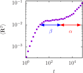
(a)  (b)

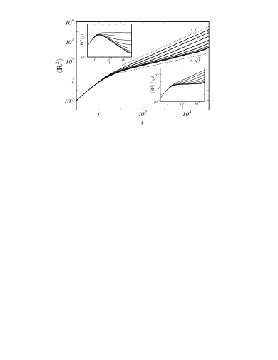
Figure 1: Behavior of the MSD, showing two-step relaxation. The time $t$ and the MSD are nondimensionalized with $\sigma^{2}/D$ and $\sigma^{2}$, respectively. (a) A three-dimensional system, densely packed with particles subject to Newtonian dynamics with thermostat[13]. (b) SFD with overtaking allowed [$V_{\text{max}}/{k_{\text{B}}}T=1,2,3,\ldots$, up to $8$; see the text below Eq. (2.1)]. The insets show the MSD compensated by $t$ and $\sqrt{t}$.

The slowness of the $\alpha$ and $\beta$ relaxations is expected to have its origin in cooperative motions of the particles, correlated both in space and time. Numerical simulations have revealed spatiotemporally nonuniform relaxation referred to as dynamical heterogeneity[7, 8], as well as vortical motions[14, 15, 16] and string motions[17]. In order to capture such cooperative relaxation processes, various space-time correlations have been devised. A popular idea is to define four-point space-time correlations by analogy with spin glasses[4, 18, 19], while there are different ideas that involve particle tracking, such as the bond breaking correlation[7, 20, 21]. Combining the idea of continuum-based particle tracking[22] with that of four-point space-time correlations[23], we find that displacement correlation[14, 24] can be quite useful.

The present article aims to give some insights into space-time correlations characterizing cooperativity in glassy liquids, by studying a simpler model of caged dynamics. By “a simpler model” we mean the one-dimensional (1D) version of Eq. (1.1), whose behavior is known as single-file diffusion (SFD). An example of SFD with large but finite interaction potential is shown in Fig. 1(b). Here the MSD exhibits two-step behavior, similar to the one shown in Fig. 1(a), though there is a difference that the “$\beta$ relaxation” in standard SFD takes the form of a subdiffusive regime with $\left\langle{R^{2}}\right\rangle\propto\sqrt{t}$ and not a plateau. For the limiting case of infinite interaction potential, the $\alpha$ relaxation disappears so that the 1D cages become eternal. If $L$ is finite, eventually the correlated motion dominates the whole system and the MSD grows again in proportion to $t$, though much more slowly than in the free diffusion[25, 26, 27, 28].

The article is organized as follows. Basics of SFD are reviewed in Sec. 2, with emphasis on cooperativity rather than anomalous diffusion. After a survey of certain approaches to SDF in Sec. 3, we introduce in Sec. 4 what we call the Alexander–Pincus (AP) formula[22, 23, 29], to calculate the displacement correlation as well as the MSD as its special case. Improvements over the original version of the formula[29] are discussed and the formula is extended to the two-dimensional (2D) case, which is the main result of the present work. Applying the AP formula to the nonlinear dynamics of 1D colloidal liquids, we improve the calculation of the MSD in Sec. 5. Preliminary results in 2D colloidal liquids are discussed in Sec. 6.

2 Basic Properties of Single-File Diffusion

2.1 Subdiffusive behavior

SFD is an old problem[30, 31] but remains an active topic. In particular, there are a number of works on SFD motivated by interest in glassy dynamics[22, 23, 25, 32, 33, 34]. SFD is also related to a study on polymeric entanglement[35] and the idea of a figure-eight model for kinetic arrest[36].

Here we consider the Brownian SFD, governed by the Langevin equation,

$$m\ddot{X}_{i}=-\mu\dot{X}_{i}-\frac{\partial}{\partial X_{i}}\sum_{j<k}V(X_{k}-X_{j})+\mu f_{i}(t),$$ (2.1)

which is the 1D version of Eq. (1.1), with $X_{i}=X_{i}(t)$ denoting the position of the $i$-th particle. The interparticle potential $V(r)$ defines the particle diameter $\sigma$, and $V_{\text{max}}=\max{V(r)}$ can be either finite or infinite.

Denoting the displacement of the $j$-th particle with $R_{j}(t)=X_{j}(t)-X_{j}(0)$, let us review the behavior of the MSD, $\left\langle{R^{2}}\right\rangle$, in the overdamped regime ($t\gg{m/\mu}$). Setting $V(r)=0$ results in free diffusion subject to Eq. (1.3), while the case with $V_{\text{max}}=+\infty$, in which overtaking is forbidden, is subdiffusive. The long-time behavior of the MSD for $V_{\text{max}}=+\infty$ is described by the Hahn–Kärger–Kollmann (HKK) law[37, 38],

$$\left\langle{R^{2}}\right\rangle\simeq\frac{2S}{\rho_{0}}\sqrt{\frac{{D^{\text{c}}}t}{\pi}},$$ (2.2)

where $S=S(k\to 0)$ is the long-wave limiting value of the static structure factor

$$S(k)=\frac{1}{N}\sum_{i,j}\left\langle{\exp\left[\mathrm{i}{k}\left(X_{j}-X_{i}\right)\right]}\right\rangle\quad(k\neq 0),$$ (2.3)

and $D^{\text{c}}=D^{\text{c}}(k\to 0)$ is that of the collective diffusion coefficient, $D^{\text{c}}(k)$, given by $D^{\text{c}}=D/S$ in the absence of hydrodynamic interaction[39, 40]. Large but finite values of $V_{\text{max}}$, as well as finite channel width in quasi-1D systems, allow overtaking[41, 42, 43, 44], which introduces the “$\alpha$ relaxation” resulting in the two-step behavior in Fig. 1. Details of the transitional behavior in quasi-1D systems depend on the softness of the confinement[41, 43]. The effect of the confinement has been studied through the cross-sectional density profile[41] and also through calculation of the free energy barrier from the configurational integral[43, 44].

It may be worth noting that there are several extensions of SFD to which the HKK law (2.2) does not apply. The HKK law is premised on statistical uniformity of the system, absence of long-range interactions, and validity of description by the Langevin equation (2.1) with constant $\mu$ and uncorrelated random forcing. Without these premises, the HKK law may well be modified. Flomenbom and Taloni[45] studied the case in which the initial distribution of the particles is inhomogeneous, in such a way that one tagged particle is located at $X_{0}=0$ and other particles are arranged around it according to the relation $X_{\pm{j}}\propto\pm j^{1/(1-a)}$ with $0\leq a\leq 1$, so that the density decreases as the distance from the tagged particle increases. In this case, $\left\langle{[R_{0}(t)]^{2}}\right\rangle$ grows in proportion to $t^{(1+a)/2}$, which interpolates between the standard HKK law (2.2) and Eq. (1.3) for free Brownian particles[45]. The analysis was extended to the cases of a heterogeneous single file with distributed diffusion coefficient[46] and “anomalous” single files whose elementary process involves power-law distribution of waiting time[45, 46, 47]; the MSD in these cases can be slower than $t^{1/2}$, and even becomes as slow as $(\log{t})^{2}$ in extreme cases[48]. Some other mechanisms, such as blocking at a junction[36] or spatially correlated noise[28], can make the diffusion so slow that a plateau may appear in the logarithmic plot of the MSD. It is also suspected that the HKK law (2.2) may break down in regard to longtime behavior of extremely dense single files[27, 34]. In the following discussion of SFD, however, we will mainly focus on the standard case in which the HKK law is valid.

For later convenience, we introduce the length scale $\ell_{0}$, expressing the mean distance between neighboring particles, by $\rho_{0}=N/L^{n_{\text{d}}}=1/\ell_{0}^{n_{\text{d}}}$. With $\ell_{0}$ introduced, we also define $D_{*}\stackrel{{\scriptstyle\text{def}}}{{=}}D/\ell_{0}^{2}$ and $D^{\text{c}}_{*}\stackrel{{\scriptstyle\text{def}}}{{=}}D^{\text{c}}/\ell_{0}^{2}$, so that $1/D^{\text{c}}_{*}$ gives a timescale at which $\sqrt{{D^{\text{c}}}t}$ becomes comparable to $\ell_{0}$. For 1D systems of rigid spheres, we have $\ell_{0}=1/\rho_{0}=L/N$ and $D^{\text{c}}_{*}(k)\simeq\rho_{0}^{2}D[1+(2\rho_{0}/k)\sin{{\sigma}k}]$.

2.2 Cooperativity in single file

While many studies on SFD now focus on the anomalous diffusion, it should be emphasized that another aspect of SFD was noticed as early as in 1955, when Hodgkin and Keynes[30] reported their experiments on potassium ion permeability across the membranes of giant axons from Sepia officinalis. They measured the $\mathrm{K^{+}}$ fluxes through the membrane in opposite directions, $Q_{\mathrm{{out}\to{in}}}$ and $Q_{\mathrm{{in}\to{out}}}$, and compared their ratio with Ussing’s equation[49] (reminiscent of the fluctuation theorem[50]):

$$\frac{Q_{\mathrm{{out}\to{in}}}}{Q_{\mathrm{{in}\to{out}}}}=\exp\left(\frac{n\Delta\Phi}{{k_{\text{B}}}T}\right),$$ (2.4)

where $\Delta\Phi=q(E_{\text{out}}-E_{\text{in}})-{k_{\text{B}}}T\log({\rho_{\text{in}}}/{\rho_{\text{out}}})$ is the electrochemical potential difference, with $q$ denoting the charge of $\mathrm{K^{+}}$; the electric potential and the ion density on the side $a$ are denoted with $E_{a}$ and $\rho_{a}$, respectively. Independent diffusion of ions should give $n=1$, while the experimental value was $n=2.5>1$, indicating some kind of cooperativity. “In a stroke of genius” (if we borrow the words by Hille[51]), forty years before crystallographic determination of ion channel structure, they said that the experimental result can be explained by assuming that $\mathrm{K^{+}}$ ions tend to move in narrow channels.

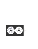
(a) (b)

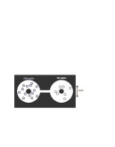
Figure 2: Experimental setup of models with granular particles (iron balls with $\sigma=3\,\mathrm{mm}$) to simulate diffusion of ions through a channel; adopted from Fig. 8 of Ref. 30 with modification. The gap length is minimal in (a), while the gap is elongated in (b) to form a long pore.

To demonstrate this idea, Hodgkin and Keynes[30] performed a mechanical experiment with granular models illustrated in Fig. 2. Causing random motion of particles by shaking the system, they observed fluxes between the chambers 1 and 2 and compared their ratio with Eq. (2.4), which reduces to ${Q_{1\to 2}}/{Q_{2\to 1}}=(\rho_{1}/\rho_{2})^{n}$ for electrically neutral particles. The experiment with a short gap in Fig. 2(a) gave the ratio close to $\rho_{1}/\rho_{2}=100/50=2$, implying nearly independent diffusion ($n\approx 1$). Contrastively, for a longer gap in Fig. 2(b), $Q_{1\to 2}$ was 18 times greater than $Q_{2\to 1}$, indicating that about four particles were cooperating ($n=\log_{2}{18}\simeq 4.2$).

In regard to ion transport across membranes, researchers have also investigated possibilities other than the long pore, assuming cooperativity on the side of the transporting proteins and not among the transported ions, which, however, turned out to be unsuccessful[52]. The “knock-on” mechanism among the $\mathrm{K^{+}}$ ions is already cooperative, and leads to the high sensitivity of the flux ratio to $\Delta{\Phi}$. In this case, the system size is finite, and the correlation length can span the entire system.

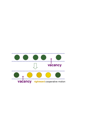
(a)​  (b)​

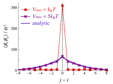
Figure 3: Cooperative motion in 1D systems. (a) Schematic description of cooperative motion due to a diffusing vacancy. (b) Numerically calculated two-particle displacement correlation $\left\langle{{R_{i}}{R_{j}}}\right\rangle$ in SFD for different values of $V_{\text{max}}$, with $N=10^{4}$, $\rho_{0}=N/L=0.2\,\sigma^{-1}$, and the time interval $t=200\,\sigma^{2}/D$; cited from Ref. 44. The analytical solution is given by Eq. (5.7).

In situations with $L\to+\infty$, including the case in which the HKK law (2.2) holds, the cooperativity exhibits itself through slow diffusion. Cooperativity is usually detected by comparing two configurations at different times, as is illustrated in Fig. 3(a). Here, the leftward diffusion of the vacancy induces rightward cooperative displacement of particles. This cooperative motion can be quantified by calculating displacement correlation[23, 24, 44], given by $\left\langle{{R_{i}}{R_{j}}}\right\rangle$ in the 1D case.

A numerical example of displacement correlation[44] is shown in Fig. 3(b). The cases with $V_{\text{max}}={k_{\text{B}}}T$ and $V_{\text{max}}=5{k_{\text{B}}}T$ are compared. After sufficiently long equilibration, the particles were renumbered consecutively at $t=0$, and the values of $\left\langle{{R_{i}}{R_{j}}}\right\rangle$ were calculated for $t=200\,\sigma^{2}/D$. In the case of relatively low barrier ($V_{\text{max}}={k_{\text{B}}}T$), the displacements of the neighboring particles are nearly uncorrelated, indicating that the particles are diffusing almost freely. Contrastively, in the case of higher barrier ($V_{\text{max}}=5{k_{\text{B}}}T$), positive correlation is observed within some finite distance. This correlation demonstrates dynamical structure behind the slow diffusion. The dynamical correlation length is diffusive and given by $\lambda(t)=2\sqrt{{D^{\text{c}}}t}$.

3 Theories of SFD: extensible to higher dimensions?

There are various theoretical approaches to SFD. Some techniques, such as the Jepsen line[53, 54, 55], highly depend on the 1D geometry, while other techniques may be extensible to three-dimensional (3D) colloidal liquids. We look for the latter kind of approaches, requiring in addition that the theory should incorporate cooperativity.

For the sake of simplicity, in the present section, sometimes we ignore the difference between $D$ and $D^{\text{c}}=D/S$. This is strictly valid only in the limit of point particles ($\sigma\ll\ell_{0}=L/N$), but it is often possible to take the effect of finite $\sigma$ into account by reviving $S$ in an obvious way.

3.1 Phenomenological treatments of cooperative diffusion

Let us start with reviewing the idea of Rallison[25] that relates the slow diffusion to cooperativity. If $n$ Brownian particles are strongly interacting and moving together, the diffusion coefficient for their center of mass is $D/n$, in the sense that

$$\frac{\mathrm{d}}{\mathrm{d}{t}}\left\langle{R^{2}}\right\rangle=\frac{2D}{n}.$$ (3.1)

To apply Eq. (3.1) to the collective dynamics in SFD, Rallison[25] proposed to replace $n$ in the denominator with $\mathcal{N}(\lambda)=1+\rho_{0}\lambda$, which is the number of particles within the dynamical correlation length $\lambda=\lambda(t)$, so that the MSD is given by

$$\left\langle{R^{2}}\right\rangle=\int_{0}\frac{2D\mathrm{d}{t}}{\mathcal{N}(\lambda)},\quad\lambda=\lambda_{\text{Ral}}^{\text{1D}}(t)=\sqrt{{4\pi}{D^{\text{c}}}t}.$$ (3.2)

Upon integration, Eq. (3.2) yields

$$\left\langle{R^{2}}\right\rangle=\frac{2S}{\rho_{0}}\sqrt{\frac{{D^{\text{c}}}t}{\pi}}-\frac{S}{\pi\rho_{0}^{2}}\log\,\left(1+\rho_{0}\sqrt{{4\pi}{D^{\text{c}}}t}\,\right);$$ (3.3)

it gives free diffusion for small $t$, and subdiffusion for large $t$ with a logarithmic correction term.

It is interesting to test Rallison’s idea in the case of a single file with non-uniform initial condition[45], given by $X_{0}(0)=0$ and $X_{\pm{j}}(0)\propto\pm j^{1/(1-a)}$. Since $\mathcal{N}(\lambda)\propto\lambda^{1-a}\propto t^{(1-a)/2}$ in this case, Eq. (3.2) readily yields $\left\langle{R^{2}}\right\rangle\propto t^{(1+a)/2}$. This result was derived by Flomenbom and Taloni[45] with an analogous but slightly different approach, in which $\mathcal{N}(\left|{R}\right|)$ was considered instead of $\mathcal{N}(\lambda)$.

Rallison[25] applied this idea to the 3D colloidal liquid and obtained a critical volume fraction, $\phi_{\text{c}}=0.64$ (with $\phi$ related to $\rho_{0}$ by $\phi={\frac{4}{3}}\pi(\frac{\sigma}{2})^{3}\rho_{0}$), above which the MSD cannot grow to infinity. This is greater than the experimental value of glass transition point ($\phi_{\text{glass}}=0.56$ according to Pusey and van Megen[56]), and rather near to the random close packing density. The discrepancy casts doubt on quantitative validity of the theory, but the idea of relating the slow diffusion to the number of particles in cooperative motion remains quite suggestive.

Another instructive idea is found in the lattice SFD by van Beijeren et al.[26]. On the basis of the picture of migrating vacancies, i.e. the discrete version of Fig. 3(a), they calculated velocity autocorrelation of the tagged particle as

$$\left\langle{u(t)u(0)}\right\rangle\simeq-A_{u}t^{-3/2}$$ (3.4)

for large $t$, where $u$ denotes the velocity and $A_{u}$ is a constant that depends on the hopping rate, concentration, and lattice constant. With the aid of the relation

$$\frac{\mathrm{d}^{2}\left\langle{R^{2}}\right\rangle}{\mathrm{d}{t}^{2}}=2\left\langle{u(t)u(0)}\right\rangle,$$ (3.5)

Eq. (3.4) readily leads to the asymptotic law, $\left\langle{R^{2}}\right\rangle\propto\sqrt{t}$.

The velocity autocorrelation in Eq. (3.4) has a negative longtime tail: the particles are always pushed back by its neighbors. The negative tail can be derived also on the basis of continuum description[57], as will be reviewed later in Eq. (3.15).

Within the framework of lattice dynamics, the idea of migrating vacancies can be applied also to geometries other than the 1D chain, such as double-file diffusion[58] and 2D regular lattices[59]. The idea of clarifying slow dynamics by moving defects has been incarnated also in free-volume kinetic models of glasses and granular matters[4, 60]. An interesting question is whether this approach can be generalized to systems without lattice, such as the one shown in Fig. 3(a). The answer is affirmative in our opinion, as will be explained in the latter half of this article.

The theory of Rallison[25] and that of van Beijeren et al.[26] were immediately applied to SFD on a ring with finite $L$. The longtime behavior in this case is given by Eq. (3.1) with $n=N$.

3.2 Density correlation in the Fourier space

As the dynamical correlation length in Brownian SFD is diffusive, it is natural to seek indication of collective motions in the density field subject to a stochastic diffusion equation. Here we review several ideas for relating the motion of a tagged particle to the density fluctuations of the medium, including the celebrated theory by Alexander and Pincus[29].

Let us define the (microscopic) density field by

$$\rho=\rho(x,t)=\sum_{i}\rho_{i},\quad\rho_{i}=\rho_{i}(x,t)=\delta(x-X_{i}(t))$$ (3.6)

where $\rho_{i}$ is the single-body density of the $i$-th particle. Evidently, $\rho$ satisfies the continuity equation

$$\partial_{t}\rho+\partial_{x}{Q}=0,$$ (3.7)

with the flux $Q={\rho}u$ given by

$$Q=Q(x,t)=\sum_{i}\rho_{i}(x,t)\dot{X}_{i}(t).$$ (3.8)

Anticipating a linear equation for $\rho(x,t)$ as a starting point and assuming that the system is translationally invariant, we introduce the Fourier representation:

$$\hat{\rho}(k,t)={\frac{1}{L}}\int e^{{\mathrm{i}}kx}\left[\rho(x,t)-\rho_{0}\right]\mathrm{d}{x},\quad\rho(x,t)=\rho_{0}+\sum_{k}\hat{\rho}(k,t)e^{-{\mathrm{i}}kx},$$ (3.9)

with $k/\Delta{k}\in\mathbb{Z}$ where $\Delta{k}=2\pi/L$.

The two-time correlation of $\hat{\rho}$ is referred to as the intermediate scattering function and essentially equivalent to the dynamical structure factor[61], as

$$F(k,t)=\frac{1}{N}\sum_{i,j}\left\langle{e^{-\mathrm{i}{k}\left[X_{i}(t)-X_{j}(0)\right]}}\right\rangle\propto\left\langle{{\hat{\rho}(k,t)}{\hat{\rho}(-k,0)}}\right\rangle\quad(k\neq 0);$$ (3.10)

the self part of $F$ gives the Fourier representation of the diffusion propagator,

$$F_{\text{S}}(k,t)=L^{2}\left\langle{\hat{\rho}_{j}(k,t)\hat{\rho}_{j}(-k,0)}\right\rangle=\left\langle{e^{\mathrm{i}{k}{R_{j}(t)}}}\right\rangle,$$ (3.11)

where $\hat{\rho}_{j}(k,t)=L^{-1}\exp\left[\mathrm{i}kX_{j}(t)\right]$ is the Fourier component of $\rho_{j}(x,t)$.

Now let us proceed to the dynamics of $\rho$. If the particles are subject to the Langevin equation (2.1) and attention is focused on the timescale longer than $m/\mu$, then $\rho$ is governed by a nonlinear stochastic equation referred to as the Dean–Kawasaki equation[62, 63, 64]. Here we discuss the linear dynamics only, deferring the nonlinear case until Sec. 5. The linear stochastic equation for $\rho$, sometimes referred to as the diffusion-noise equation[1, 57], reads

$$\partial_{t}\rho(x,t)=D\partial_{x}^{2}\rho+f_{\rho}(x,t),$$ (3.12)

with the statistics of the noise term given by

$$\left\langle{f_{\rho}(x,t)f_{\rho}({x^{\prime}},{t^{\prime}})}\right\rangle =2D\partial_{x}\partial_{x^{\prime}}\rho(x,t)\delta(x-x^{\prime})\delta(t-t^{\prime})$$

$$\simeq 2\rho_{0}D\partial_{x}\partial_{x^{\prime}}\delta(x-x^{\prime})\delta(t-t^{\prime}).$$ (3.13)

The linearized Dean–Kawasaki equation (3.12) is readily solved in the Fourier representation. With this solution, Taloni and Lomholt[57] calculated the velocity autocorrelation, $\left\langle{{u_{j}(t)}{u_{j}(0)}}\right\rangle$ with $u_{j}=\dot{X}_{j}$, which is related to the MSD by Eq. (3.5). The single-file condition implies that the velocity of the tagged particle equals that of the medium around it (for the timescale longer than $1/D_{*}$), so that

$$u_{j}(t)=u(X_{j}(t),t)\simeq u(X_{j}(0),t)=\frac{Q(X_{j}(0),t)}{\rho_{0}}.$$ (3.14)

The replacement of $X_{j}(t)$ by $X_{j}(0)$ is justified by the relative smallness of the displacement in comparison to the dynamical correlation length. Using the continuity equation (3.7) and the space-time Fourier transform of the noise term, they found[57]

$$\left\langle{{u(t)}{u(0)}}\right\rangle=-\frac{1}{4\rho_{0}}\sqrt{\frac{D}{{\pi}t^{3}}},$$ (3.15)

reproducing the same negative longtime tail as in Eq. (3.4). We note that the negative tail in the velocity autocorrelation is a manifestation of the cage effect, found in 2D and 3D colloidal systems as well[40, 65], and differs from the positive longtime tail reported by Alder and Wainwright[66].

Taloni and Lomholt[57] also succeeded in interpolating the longtime collective dynamics in SFD and the short-time single-particle behavior, describing the velocity of the particle with a generalized Langevin equation

$$m\frac{\mathrm{d}{u}}{\mathrm{d}{t}}=-\int_{0}^{t}K(t-t^{\prime})u(t^{\prime})\mathrm{d}{t^{\prime}}+f_{K}(t),$$ (3.16)

where $f_{K}$ is a time-correlated noise related to the kernel $K$ by the relation

$$\left\langle{{f_{K}(t)}{f_{K}(t^{\prime})}}\right\rangle={m{k_{\text{B}}}T}K(\left|{t-t^{\prime}}\right|).$$ (3.17)

The longtime behavior of $K$ can be determined by Fourier analysis of the collective dynamics in Eq. (3.12) or its chain-dynamical equivalent[1, 57, 67]. Furthermore, the short-time behavior should reduce to that of a free Brownian particle. By incorporating these two limiting cases into $K$, Taloni and Lomholt[57] obtained

$$\left\langle{R^{2}}\right\rangle\simeq\frac{1}{\rho_{0}^{2}}\left[2\sqrt{\frac{{D_{*}}t}{\pi}}+\frac{e^{4{D_{*}}t}}{2}\operatorname{erfc}\left(2\sqrt{{D_{*}}t}\,\right)-\frac{1}{2}\right].$$ (3.18)

Contrastively, the concise theory by Alexander and Pincus[29] avoids directly dealing with the velocity $u$ and relates the MSD directly to the density fluctuation, by the integral

$$\left\langle{R^{2}}\right\rangle\propto\int\frac{1-e^{-Dk^{2}t}}{k^{2}}\mathrm{d}{k}.$$ (3.19)

We refer to Eq. (3.19) and its extensions as the Alexander–Pincus (AP) formula.

The original derivation of Eq. (3.19) is traced as follows: Let $h_{j}=h_{j}(t)$ denote the displacement of the $j$-th particle from a configuration in which the particles are uniformly distributed, so that $h_{j}(t)=X_{j}(t)-j\ell_{0}$. Rewriting $\hat{\rho}(k,t)$ with $h_{j}$ as

$$\hat{\rho}(k,t)=\sum_{j}\hat{\rho}_{j}(k,t)={\frac{1}{L}}\sum_{j}e^{\mathrm{i}{k}\left[j\ell_{0}+h_{j}(t)\right]}\quad(k\neq 0)$$ (3.20)

and introducing $\hat{h}(k,t)={\frac{1}{N}}\sum_{j}e^{{\mathrm{i}}kj\ell_{0}}h_{j}(t)$ so that $h_{j}(t)=\sum_{k}\hat{h}(k,t)e^{-{\mathrm{i}}kj\ell_{0}}$, one expands $\hat{\rho}(k,t)$ in Eq. (3.20) in power series of $kh_{j}(t)$, to find

$$\hat{\rho}(k,t)={\frac{1}{L}}\sum_{j}e^{\mathrm{i}{k}j\ell_{0}}\left[1+{\mathrm{i}}kh_{j}(t)+O(k^{2}h_{j}^{2})\right]\simeq{\mathrm{i}}k\rho_{0}\hat{h}(k,t).$$ (3.21)

By noticing $R_{j}(t)=h_{j}(t)-h_{j}(0)$ and using Eq. (3.21), the MSD is calculated as

$$\left\langle{R_{j}^{2}}\right\rangle=2\left\{\left\langle{\smash{\left[h_{j}(0)\right]^{2}}}\right\rangle-\left\langle{h_{j}(t)h_{j}(0)}\right\rangle\right\}\propto\sum_{k}\frac{F(k,0)-F(k,t)}{k^{2}};$$ (3.22)

then, replacing the summation with an integral and substituting $F(k,t)\propto e^{-Dk^{2}t}$, we arrive at Eq. (3.19), from which $\left\langle{R^{2}}\right\rangle\propto\sqrt{t}$ is readily obtained.

It should be noted that the above derivation includes a step requiring attention. Since $h$ is not small, the validity of the expansion in Eq. (3.21) poses a delicate issue. However, this difficulty is avoided by using a convected coordinate system, as will be shown in Sec. 4.

3.3 Mode-coupling theory

Conceptually, the generalized Langevin equation (3.16) could be regarded as projection of the $N$-body equation (2.1) onto the single-particle motion. However, this projection seems to be difficult to perform systematically in the real space (as oppose to the Fourier space)[1]. It is then interesting to notice the case in which the Mori–Zwanzig projection formalism has been applied to 3D dynamics of glassy liquids, known by the name of mode-coupling theory (MCT)[12, 68, 69]. Projection of the equation of motion onto the density correlation $F$ yields

$$\left(\partial_{t}+D^{\text{c}}k^{2}\right)F(k,t)=-\int_{0}^{t}M(k,t-t^{\prime})\partial_{t^{\prime}}F(k,t^{\prime})\mathrm{d}{t^{\prime}},$$ (3.23)

which is then closed by approximating the memory kernel $M$ with a quadratic functional of $F$. In spite of various limitations, the MCT equation has succeeded in reproducing the two-step relaxation of $F(k,t)$ and the growth of the relaxation time, as the mean density $\rho_{0}$ increases[10, 11, 12].

Diffusion of a tagged particle is treated by the MCT equation for $F_{\text{S}}$, in the form

$$\left(\partial_{t}+Dk^{2}\right)F_{\text{S}}(k,t)=-\int_{0}^{t}M_{\mathrm{S}}(k,t-t^{\prime})\partial_{t^{\prime}}F_{\text{S}}(k,t^{\prime})\mathrm{d}{t^{\prime}},$$ (3.24)

with the memory kernel $M_{\mathrm{S}}$ expressed as a bilinear functional of $F$ and $F_{\text{S}}$. In description of SFD with Eq. (3.24), however, it is difficult to reproduce the $\sqrt{t}$ behavior. As long as the standard memory kernel is used, MCT cannot predict anomalous diffusion[33]. Mathematical difficulty is located in constructing $M_{\mathrm{S}}$ with proper longtime behavior, which is actually more difficult than constructing $K$ in Eq. (3.16), because $K$ can be given before the unknown $u$ is determined, while $M_{\mathrm{S}}$ must be a functional of the unknown $F$ and $F_{\text{S}}$. In modified MCT approaches by Fedders[70] and Abel et al.[33], $M_{\mathrm{S}}$ is improved by taking the prohibition of positional exchanges directly into account; as a result, the correct $t^{1/2}$-law is recovered.

Another possible approach consists of retaining Eq. (3.23) for $F$ alone, while Eq. (3.24) for $F_{\text{S}}$ is replaced with another equation for tracers, in which the four-point correlation is directly taken into account[35, 38]. We will see that an improved version of the AP formula is suitable for this purpose[23].

3.4 Elastic chains

The longtime dynamics of SFD are known to be equivalent to those of fluctuating elastic chains. The linear dynamics are then described by replacing $V(X_{k}-X_{j})$ in Eq. (2.1) with the harmonic effective potential, so that the equation of motion reads

$$m\ddot{X}_{i}+\mu\dot{X}_{i}=\kappa\left(X_{i+1}-2X_{i}+X_{i-1}\right)+\mu f_{i}(t)$$ (3.25)

with $\kappa$ denoting the effective spring constant[67, 71]. Taking the continuous limit and considering the overdamped case ($m\to 0$) for simplicity, we rewrite Eq. (3.25) in terms of $x(\xi,t)$, with $\xi$ here denoting a continuum analogue of $i$:

$$\partial_{t}{h(\xi,t)}=D^{\prime}\partial_{\xi}^{2}{h(\xi,t)}+f_{h}(\xi,t),$$ (3.26)

where $D^{\prime}=\kappa/\mu$ and $\left\langle{{f_{h}(\xi,t)}{f_{h}(\xi^{\prime},t^{\prime})}}\right\rangle=2D\delta(\xi-\xi^{\prime})\delta(t-t^{\prime})$. Note that $h$ can be taken equal to the position $x$ itself, as $h=x(\xi,t)$, or the displacement from the mean position, as $h=x(\xi,t)-\ell_{0}\xi$. In any case, the displacement is given by $R(\xi,t)=h(\xi,t)-h(\xi,0)$, and the MSD is given by the essentially same integral as Eq. (3.19). The Langevin equation for elastic chains is known as the Rouse model in the context of polymer dynamics[72]. The dynamics of a curve $h=h(\xi,t)$ on the $(\xi,h)$ plane can also be interpreted as kinetic roughening of a fluctuating surface[24, 73], with Eq. (3.26) referred to as the Edwards–Wilkinson equation[74, 75].

While this reduction to elastic chain seems obvious in the case of soft-core interaction, the important point is that also the hardcore interaction can be described by a smooth effective potential between the particles, as a result of coarse-graining in time. Recently, this point has been discussed both in the 1D setup[67] and in the context of glassy liquids in higher dimensions[15, 76], seemingly by independent groups. The effective potential, calculated from the partition function that gives the free energy, is of entropic origin: the interparticle force is essentially the osmotic pressure of the ideal solution, i.e. the pressure of the ideal gas.

The discrete equation (3.25) and its higher-dimensional analogues are amenable to normal mode analysis[2, 15, 16], which is often performed around some metastable configuration. Modes with low frequencies are found to be important. In the case of colloidal glass with ${n_{\text{d}}}\geq 2$, the presence of the low-frequency modes is related to the character of the interaction described by the “bonds”, which can directly sustain compression but not necessarily resist shear deformation. In the continuum description, the normal modes are plane waves. In correspondence to the low-frequency modes in discrete systems, the continuum description of colloidal liquids must respect the distinction between the longitudinal and transverse modes.

The situation can be simpler in systems that are elastic by nature, such as an assembly of densely packed softcore particles or a system of colloidal particles trapped in a polymeric network. In such models, the presence of finite rigidity could be taken for granted, so that simplified description based on the scalar integral

$$\left\langle{R^{2}}\right\rangle\propto\int\frac{1-e^{-Dk^{2}t}}{k^{2}}\,\mathrm{d}^{n_{\text{d}}}{\mathbf{k}}\qquad(\text{without tensorial treatment})$$ (3.27)

might be justifiable. Once the description by the linear elastic model is justified, it allows analytical calculation of displacement correlation and even some four-point correlations such as dynamical susceptibility[77]. Details will be discussed elsewhere.

The effect of dimensionality on the MSD in elastic models may deserve some comments. The 1D AP formula is free from ultraviolet divergence, while $t$ must be finite to avoid infrared divergence of the MSD. In the 2D and 3D cases, a ultraviolet cutoff must be introduced. Denoting the cutoff wavenumber with $k_{0}=\tilde{k}_{0}/\ell_{0}$, we calculate the MSD in the 2D case from Eq. (3.27) as

$$\left\langle{\mathbf{R}^{2}}\right\rangle\propto\log\left(1+\tilde{k}_{0}^{2}{D^{\text{c}}_{*}}t\right),$$ (3.28)

and for ${n_{\text{d}}}=3$ we find

$$\left\langle{\mathbf{R}^{2}}\right\rangle\propto 1-\frac{1}{\sqrt{1+\tilde{k}_{0}^{2}{D^{\text{c}}_{*}}t}}.$$ (3.29)

The large $t$ behavior of Eq. (3.28) differs from that of Eq. (3.29): the MSD for ${n_{\text{d}}}=3$ converges for $t\to+\infty$, while that for ${n_{\text{d}}}=2$ diverges logarithmically, until the effect of the finite system size comes into play at $t\sim L^{2}/D^{\text{c}}$. Thus the 2D elastic model suffers both infrared and ultraviolet divergences. It can be even argued that the 2D harmonic solid is not a solid in the usual sense[78], at least if one accepts the argument that single-file systems are denied to be solid because any particle in the system can get arbitrarily far away from its initial position[79].

4 Alexander–Pincus Formula in Convected Coordinate System

We have reviewed several theories of SFD that may be extensible to higher dimensions, including the AP formula (3.19), which relates the MSD to $F(k,t)\propto e^{-D{k^{2}}t}$. Since the original derivation of the formula is of approximate nature, it seems difficult to improve the result by considering a nonlinear correction to $F$.

Here we redevelop the AP formula, making it exact by changing the variables appropriately[22, 23]. The key to this approach is the adoption of Lagrangian correlations, motivated by theories of the Navier–Stokes turbulence[80, 81, 82]. While the formula itself remains linear with regard to the correlation in the new variables, it can be combined with a nonlinear equation of the correlation, so that the result can be improved as we will see later in Subsec. 5.3. The formula is also extended so as to give the displacement correlation in ${n_{\text{d}}}$-dimensional systems.

4.1 Label variable and the 1D AP formula

Let us start with reviewing a classic idea of the Lagrangian description in fluid mechanics. The idea is to introduce a continuous and invertible mapping

$$(\bm{\xi},t)=(\xi,\eta,\zeta,t)\mapsto\mathbf{r}=\begin{bmatrix}x(\bm{\xi},t)\\ y(\bm{\xi},t)\\ z(\bm{\xi},t)\end{bmatrix},$$ (4.1)

such that its inverse, $\bm{\xi}=\bm{\xi}(\mathbf{r},t)$, satisfies the convective equation

$$\left(\partial_{t}+\mathbf{u}\cdot\nabla\right)\bm{\xi}(\mathbf{r},t)=\mathbf{0}.$$ (4.2)

This mapping makes it possible to specify a world line as ${\bm{\xi}(\mathbf{r},t)}=\text{const.}$, and therefore we refer to $\bm{\xi}$ as the label variable. In other words, $\bm{\xi}$ is a continuum analogue of the particle numbering; as a matter of fact, the 1D label variable is a mere continuous interpolation of the consecutive numbering of the particles, but here we introduce the label variable in a more abstract way so as to enable extension to higher dimensions without postulating regular numbering at all. The moving curvilinear coordinate system given by Eq. (4.1) is sometimes referred to as the convected coordinate system[83]. The description in which the field variables are regarded as functions of $(\bm{\xi},t)$ is termed as the Lagrangian description, as opposed to the Eulerian description in which the independent variables are $\mathbf{r}$ and $t$.

There are infinitely many choices of label variable in general. In the 1D case[22, 23], we choose $\xi$ so as to satisfy

$${\partial_{x}}\xi({x},{t})=\rho,\quad{\partial_{t}}\xi({x},{t})=-Q,$$ (4.3)

where $\rho=\rho(x,t)$ and $Q=Q(x,t)$ are the density and the flux satisfying the continuity equation (3.7). It is then readily verified that $\xi=\xi(x,t)$ satisfies the 1D convective equation, which qualifies $\xi$ as a label variable.

For this particular choice of the label variable, the derivatives of $x=x(\xi,t)$ are

$$\partial_{\xi}{x(\xi,t)}=\frac{1}{\rho(\xi,t)},\quad\partial_{t}{x(\xi,t)}=\frac{Q}{\rho}=u(\xi,t).$$ (4.4)

The presence of $1/\rho$ in Eq. (4.4) motivates us to introduce the “vacancy field”

$$\psi=\psi(\xi,t)=\frac{\rho_{0}}{\rho(\xi,t)}-1,$$ (4.5)

so that the relation $\partial_{t}\partial_{\xi}{x}=\partial_{\xi}\partial_{t}{x}$ is cast into the form of the vacancy conservation,

$$\ell_{0}\partial_{t}\psi(\xi,t)=\partial_{\xi}{u(\xi,{t})}.$$ (4.6)

Then, by using $\psi(\xi,t)$ instead of $\rho(x,t)$, we can derive a more rigorous version of the AP formula[23], in the sense that the approximation in Eq. (3.21) is not required. The formula for the MSD reads

$$\left\langle{R^{2}}\right\rangle=\frac{L^{4}}{\pi N^{2}}\int_{-\infty}^{\infty}\frac{C(k,0)-C(k,t)}{k^{2}}\mathrm{d}{k}$$ (4.7)

in the statistically steady case, where

$$C(k,t)\stackrel{{\scriptstyle\text{def}}}{{=}}\frac{N}{L^{2}}\left\langle{\check{\psi}(k,t)\check{\psi}(-k,0)}\right\rangle$$ (4.8)

is the Lagrangian correlation of vacancy in Fourier representation:

$$\check{\psi}(k,t)={\frac{1}{N}}\int e^{\mathrm{i}k\xi}\psi(\xi,t)\mathrm{d}\xi,\quad\psi(\xi,t)=\sum_{k}\check{\psi}(k,t)e^{-\mathrm{i}k\xi}\quad\left(\frac{k}{2\pi/N}\in\mathbb{Z}\right).$$ (4.9)

The haček (inverted hat) is used to make a clear distinction between the two Fourier transforms exemplified by Eqs. (3.9) and (4.9). The formula for the MSD in Eq. (4.7) is a special case of the formula for the displacement correlation,

$$\left\langle{R(\xi,t)R(\xi^{\prime},t)}\right\rangle=\frac{L^{4}}{\pi N^{2}}\int_{-\infty}^{\infty}e^{-{\mathrm{i}}k(\xi-\xi^{\prime})}\frac{C(k,0)-C(k,t)}{k^{2}}\mathrm{d}{k},$$ (4.10)

where $R(\xi,t)=x(\xi,t)-x(\xi,0)$. For $\xi=\xi^{\prime}$, Eq. (4.10) reduces to Eq. (4.7).

To begin the derivation of the AP formula, we notice that

$$\partial_{\xi}{R(\xi,t,s)}=\ell_{0}\left[\psi(\xi,t)-\psi(\xi,s)\right]$$ (4.11)

where $R(\xi,t,s)=x(\xi,t)-x(\xi,s)$; this is readily verified with Eqs. (4.4) and (4.5). Integration of Eq. (4.11) in Fourier representation yields

$$R(\xi,t,s)=\ell_{0}\sum_{k}\left[\check{\psi}(k,t)-\check{\psi}(k,s)\right]\frac{e^{-\mathrm{i}{k\xi}}}{-\mathrm{i}{k}}+{{R}}_{\text{G}}(t,s),$$ (4.12)

with ${{R}}_{\text{G}}$ denoting the displacement of the center of mass, negligible for $N\to\infty$. Multiplying Eq. (4.12) by its duplicate with $(\xi,k)$ replaced by $(\xi^{\prime},-k^{\prime})$, we find

$$\left\langle{{R(\xi,t,s)}{R(\xi^{\prime},t,s)}}\right\rangle$$

$$=\ell_{0}^{2}\sum_{k}\sum_{k^{\prime}}\left\langle{\left[\check{\psi}(k,t)-\check{\psi}(k,s)\right]\left[\check{\psi}(-k^{\prime},t)-\check{\psi}(-k^{\prime},s)\right]}\right\rangle\frac{e^{-\mathrm{i}{k\xi}+\mathrm{i}{k^{\prime}\xi^{\prime}}}}{{k}{k^{\prime}}}$$

$$=\ell_{0}^{2}\sum_{k}\left\langle{\left[\check{\psi}(k,t)-\check{\psi}(k,s)\right]\left[\check{\psi}(-k,t)-\check{\psi}(-k,s)\right]}\right\rangle\frac{e^{-\mathrm{i}{k(\xi-\xi^{\prime})}}}{k^{2}};$$ (4.13)

the terms with $k\neq{k^{\prime}}$ is shown to vanish if $\psi(k,t)$ is subject to linear Langevin equation whose forcing term is uncorrelated for different wavenumbers [see Eq. (5.4), for example], and the same is true for nonlinear cases, in the limit of $N\to\infty$, as long as the vertex is sparse in Kraichnan’s sense[84, 85]. Taking continuum limit as $\sum_{k}(\cdots)\to\frac{N}{2\pi}\int(\cdots)\mathrm{d}{k}$, we obtain

$$\left\langle{{R(\xi,t,s)}{R(\xi^{\prime},t,s)}}\right\rangle\\ {}=\frac{L^{4}}{\pi{N^{2}}}\int_{-\infty}^{+\infty}\left[\frac{C(k,t,t)+C(k,s,s)}{2}-C(k,t,s)\right]\frac{e^{-\mathrm{i}{k}(\xi-\xi^{\prime})}}{k^{2}}\mathrm{d}{k}$$ (4.14)

where $C(k,t,s)\stackrel{{\scriptstyle\text{def}}}{{=}}(N/L^{2})\left\langle{\check{\psi}(k,t)\check{\psi}(-k,s)}\right\rangle$. In the statistically steady case, we can choose $s=0$ without loss of generality and, setting $C(k,t,0)=C(k,t)$, which also implies that $C(k,t,t)=C(k,s,s)=C(k,0)$, we arrive at Eq. (4.10).

The AP formula (4.10) has the advantage of being able to provide the displacement correlation, which is a four-point space-time correlation, in terms of two-body Lagrangian correlation. This is contrastive to the approach via $F_{\text{S}}$ in Eq. (3.11), which requires calculation of a four-body correlation.

4.2 AP formula in higher dimensions

The AP formula may seem to be easily extensible to higher-dimensional cases, simply with the ${n_{\text{d}}}$-dimensional wavenumber integral as in Eq. (3.27). This form, however, should not be taken literally but only as a simplified treatment in which the deformation is restricted to one of the ${n_{\text{d}}}$ modes of elastic waves[77]. As was noted in Subsec. 3.4, the description of colloidal liquids requires distinction between the longitudinal and transverse modes. Here we demonstrate how to extend the AP formula respecting this distinction, which results in a tensorial formula.

For concreteness, let us focus on the 2D case (${n_{\text{d}}}=2$). Our target is the displacement correlation tensor,

$$\left\langle{\mathbf{R}(\bm{\xi},t,s)\otimes\mathbf{R}(\bm{\xi}^{\prime},t,s)}\right\rangle=\begin{bmatrix}\left\langle{{R_{1}}{R_{1}}}\right\rangle\!&\left\langle{{R_{1}}{R_{2}}}\right\rangle\\ \left\langle{{R_{2}}{R_{1}}}\right\rangle\!&\left\langle{{R_{2}}{R_{2}}}\right\rangle\end{bmatrix}$$ (4.15)

where $R_{1}$ and $R_{2}$ are the Cartesian components of the displacement $\mathbf{R}$, with the arguments omitted when obvious. The label variable $\bm{\xi}=(\xi,\eta)$ is defined through the 2D extension of Eq. (4.3), later shown as Eq. (4.20), so that $\bm{\Xi}_{i}=\bm{\xi}(\mathbf{r}_{i}(t),t)$ is independent of $t$. Conceptually, $\ell_{0}\bm{\Xi}_{i}$ is supposed to express the mean position of the $i$-th particle (for some appropriate timescale shorter than the $\alpha$ relaxation time[76]).

The ambiguity due to non-uniqueness of $\bm{\xi}$ can be removed by introducing

$$\mathsf{X}(\tilde{\mathbf{d}},t,s)=\left\langle{\frac{1}{L^{2}}\iint\delta^{2}(\mathbf{r}_{\mathrm{B}}-\mathbf{r}_{\mathrm{A}}-\tilde{\mathbf{d}})\,\mathbf{R}_{\mathrm{A}}\otimes\mathbf{R}_{\mathrm{B}}\,{\mathrm{d}^{2}\mathbf{r}_{\mathrm{A}}}{\mathrm{d}^{2}\mathbf{r}_{\mathrm{B}}}}\right\rangle$$ (4.16)

where $\mathbf{r}_{\mathrm{A}}=\mathbf{r}(\bm{\xi}_{\mathrm{A}},s)$, $\mathbf{R}_{\mathrm{A}}=\mathbf{r}(\bm{\xi}_{\mathrm{A}},t)-\mathbf{r}(\bm{\xi}_{\mathrm{A}},s)$, and $\mathbf{r}_{\mathrm{B}}$ and $\mathbf{R}_{\mathrm{B}}$ are defined analogously. Equation (4.16) gives the two-particle displacement correlation as a function of the initial relative position vector $\tilde{\mathbf{d}}$. Approximately we have

$$\mathsf{X}(\tilde{\mathbf{d}},t,s)\simeq\left\langle{\mathbf{R}(\bm{\xi},t,s)\otimes\mathbf{R}(\bm{\xi}^{\prime},t,s)}\right\rangle$$ (4.17)

with $\tilde{\mathbf{d}}\simeq\ell_{0}(\bm{\xi}-\bm{\xi}^{\prime})$, and a correction to this approximate expression can be obtained in terms of triple correlations (see Subsec. V-A. in Ref. 23).

Recalling that our construction of the 1D label variable through Eq. (4.3) is closely connected to the 1D continuity equation (3.7), we relate the ${n_{\text{d}}}$-dimensional label variable to the ${n_{\text{d}}}$-dimensional continuity equation,

$$\partial_{t}\rho+\nabla\cdot\mathbf{Q}=0,$$ (4.18)

in a similar way. The (particle-scale) density $\rho=\rho(\mathbf{r},t)=\sum_{i}\rho_{i}$ and the corresponding flux $\mathbf{Q}=\mathbf{Q}(\mathbf{r},t)=\rho\mathbf{u}$ are given by straightforward generalization of Eqs. (3.6) and (3.8): for ${n_{\text{d}}}=2$, we have $\rho_{i}=\delta^{2}({\mathbf{r}}-\mathbf{r}_{i}({t}))$ and $\mathbf{Q}=\sum_{i}\rho_{i}({\mathbf{r}},{t})\dot{\mathbf{r}}_{i}({t})$.

To generalize Eq. (4.3) to ${n_{\text{d}}}$-dimensional cases, we write it in the form

$$(\rho,Q)=\begin{vmatrix}\mathbf{e}_{0}&{\partial_{t}}\xi\\ \mathbf{e}_{1}&{\partial_{x}}\xi\end{vmatrix}=({\partial_{x}\xi},\;{-\partial_{t}\xi}).$$ (4.19)

The above form is suggestive and motivates us to assume that $\bm{\xi}$ is related to $(\rho,\mathbf{Q})$ by the bilinear equation

$$(\rho,\mathbf{Q})=\begin{vmatrix}\mathbf{e}_{0}&\partial_{t}\xi&\partial_{t}\eta\\ \mathbf{e}_{1}&\partial_{x}\xi&\partial_{x}\eta\\ \mathbf{e}_{2}&\partial_{y}\xi&\partial_{y}\eta\end{vmatrix}=\left(\;\begin{vmatrix}\partial_{x}\xi&\partial_{x}\eta\\ \partial_{y}\xi&\partial_{y}\eta\end{vmatrix},\;\begin{vmatrix}\partial_{y}\xi&\partial_{y}\eta\\ {\partial_{t}}\xi&{\partial_{t}}\eta\end{vmatrix},\;\begin{vmatrix}{\partial_{t}}\xi&{\partial_{t}}\eta\\ \partial_{x}\xi&\partial_{x}\eta\end{vmatrix}\;\right)$$ (4.20)

for ${n_{\text{d}}}=2$, and a trilinear equation in an analogous form for the 3D case[22]. It is then verified that $\bm{\xi}$ satisfies the convective equation (4.2), if it solves Eq. (4.20). Within linear approximation in regard to $\rho-\rho_{0}$ and $\mathbf{Q}$, a solution

$$(\xi,\eta)=\frac{(x,y)}{\ell_{0}}-\ell_{0}\int_{o}^{t}\mathbf{Q}(\mathbf{r},\tilde{t})\,\mathrm{d}{\tilde{t}}+\ell_{0}\nabla\phi,\quad\nabla^{2}\phi=\rho(\mathbf{r},o)-\rho_{0}$$ (4.21)

can be constructed, where $o$ is an arbitrary “initial” time.

In the spirit of Eqs. (4.4) and (4.5) where $\psi=\psi(\xi,t)$ is introduced on the basis of $\partial{x}/\partial{\xi}=1/\rho$, we consider the deformation gradient tensor and introduce $(\Psi_{1},\Psi_{2})$ on the basis of its diagonal components, as

$$\begin{bmatrix}{\partial_{\xi}{x}}&{\partial_{\eta}{x}}\\ {\partial_{\xi}{y}}&{\partial_{\eta}{y}}\end{bmatrix}=\ell_{0}\left(\openone+\begin{bmatrix}\Psi_{1}(\bm{\xi},t)&*\\ *&\Psi_{2}(\bm{\xi},t)\end{bmatrix}\right),$$ (4.22)

where the off-diagonal components are omitted and replaced with an asterisk.

It follows from Eq. (4.22) that $\partial_{\xi}{R_{1}}(\bm{\xi},t,s)=\ell_{0}\left[\Psi_{1}(\bm{\xi},t)-\Psi_{1}(\bm{\xi},s)\right]$, with $s<t$, and an analogous expression for $\partial_{\eta}{R_{2}}$ is also readily available. Introducing the Fourier representation as

$$\begin{bmatrix}\Psi_{1}(\bm{\xi},t)\\ \Psi_{2}(\bm{\xi},t)\end{bmatrix}=\sum_{\mathbf{k}}\begin{bmatrix}\check{\Psi}_{1}(\mathbf{k},t)\\ \check{\Psi}_{2}(\mathbf{k},t)\end{bmatrix}e^{-\mathrm{i}\mathbf{k}\cdot\bm{\xi}}$$ (4.23)

with $\mathbf{k}=(k_{1},k_{2})$, which is a straightforward generalization of Eq. (4.9), we find

$$R_{1}(\bm{\xi},t,s)=\ell_{0}\sum_{\mathbf{k}}\left[\check{\Psi}_{1}(\mathbf{k},t)-\check{\Psi}_{1}(\mathbf{k},s)\right]\frac{e^{-\mathrm{i}\mathbf{k}\cdot\bm{\xi}}}{-\mathrm{i}{k_{1}}}+X_{\mathrm{G}}(t,s);$$ (4.24)

subsequently, with the fluctuation of the center of mass $\mathbf{R}_{\mathrm{G}}=(X_{\mathrm{G}},Y_{\mathrm{G}})$ neglected for $N\to\infty$, Eq. (4.24) yields

$$\left\langle{{R_{1}(\bm{\xi},t,s)}{R_{1}(\bm{\xi}^{\prime},t,s)}}\right\rangle$$

$$=\ell_{0}^{2}\sum_{\mathbf{k}}\sum_{\mathbf{k}^{\prime}}\left\langle{\left[\check{\Psi}_{1}(\mathbf{k},t)-\check{\Psi}_{1}(\mathbf{k},s)\right]\left[\check{\Psi}_{1}(-\mathbf{k}^{\prime},t)-\check{\Psi}_{1}(-\mathbf{k}^{\prime},s)\right]}\right\rangle\frac{e^{-\mathrm{i}\mathbf{k}\cdot\bm{\xi}+\mathrm{i}\mathbf{k}^{\prime}\cdot\bm{\xi}^{\prime}}}{{k_{1}}{k^{\prime}_{1}}}.$$ (4.25)

Provided that the same condition as was mentioned immediately after Eq. (4.13) is satisfied, the terms with $\mathbf{k}\neq\mathbf{k}^{\prime}$ are seen to vanish as in the 1D case. Then, taking the continuum limit, we obtain an expression that gives $\left\langle{{R_{1}}{R_{1}}}\right\rangle$ in terms of correlation of $\check{\Psi}_{1}$. Other components of the displacement correlation tensor are calculated in a similar way. Defining

$$C_{\alpha\beta}(\mathbf{k},t,s)\stackrel{{\scriptstyle\text{def}}}{{=}}\frac{N}{L^{4}}\left\langle{{\check{\Psi}_{\alpha}(\mathbf{k},t)}{\check{\Psi}_{\beta}(-\mathbf{k},s)}}\right\rangle\quad(\alpha,\beta\in\{1,2\})$$ (4.26)

and assuming $C_{\alpha\beta}$ to be real and symmetric so that $C_{21}(\pm\mathbf{k},t,s)=C_{12}(\mathbf{k},t,s)$, we find

$$\left\langle{{{R_{\alpha}}(\bm{\xi},t,s)}{{R_{\beta}}(\bm{\xi}^{\prime},t,s)}}\right\rangle\\ {}=\frac{L^{6}}{{2\pi^{2}}N}\iint\left[\frac{C_{\alpha\beta}(\mathbf{k},s,s)+C_{\alpha\beta}(\mathbf{k},t,t)}{2}-C_{\alpha\beta}(\mathbf{k},t,s)\right]\frac{e^{-\mathrm{i}\mathbf{k}\cdot(\bm{\xi}-\bm{\xi}^{\prime})}}{{k_{\alpha}}{k_{\beta}}}\mathrm{d}{k_{1}}\mathrm{d}{k_{2}},$$ (4.27)

where we can choose $\bm{\xi}^{\prime}=\mathbf{0}$ without loss of generality.

For later convenience, let us rewrite the 2D AP formula in terms of the dilatational and rotational modes of deformation. We define

$$\psi_{\mathrm{d}}(\mathbf{k},t) =\check{\Psi}_{1}(\mathbf{k},t)+\check{\Psi}_{2}(\mathbf{k},t),$$ (4.28a)

$$\psi_{\mathrm{r}}(\mathbf{k},t) =\frac{k_{1}}{k_{2}}\check{\Psi}_{1}(\mathbf{k},t)-\frac{k_{2}}{k_{1}}\check{\Psi}_{2}(\mathbf{k},t),$$ (4.28b)

so as to have the Fourier representation of the dilatational and rotational modes:

$$\partial_{\xi}{x}+\partial_{\eta}{y}=\ell_{0}\left(2+\sum_{\mathbf{k}}\psi_{\mathrm{d}}(\mathbf{k},t)e^{-\mathrm{i}\mathbf{k}\cdot\bm{\xi}}\right),\quad\partial_{\xi}{y}-\partial_{\eta}{x}=\ell_{0}\sum_{\mathbf{k}}\psi_{\mathrm{r}}(\mathbf{k},t)e^{-\mathrm{i}\mathbf{k}\cdot\bm{\xi}}.$$ (4.29)

The correlations of these modes are denoted by

$$C_{ab}(\mathbf{k},t,s)=\frac{N}{L^{4}}\left\langle{{\psi_{a}(\mathbf{k},t)}{\psi_{b}(-\mathbf{k},s)}}\right\rangle$$ (4.30)

with $a,b\in\{\mathrm{d},\mathrm{r}\}$ and $s<t$. Obviously, $C_{\alpha\beta}$ in Eq. (4.26) can be expressed as a linear combination of $C_{ab}$ in Eq. (4.30), and vice versa. For simplicity, let us assume that $C_{\mathrm{rd}}$ and $C_{\mathrm{dr}}$ vanish identically for some reason (such as the parity), and denote $C_{\mathrm{dd}}$ by ${C}_{\mathrm{d}}$ and $C_{\mathrm{rr}}$ by ${C}_{\mathrm{r}}$. Then the relation between $C_{\alpha\beta}$ and $C_{a}$ reads

$$\begin{bmatrix}C_{11}&C_{12}\\ C_{21}&C_{22}\end{bmatrix}=\frac{1}{\mathbf{k}^{4}}\begin{bmatrix}k_{1}^{4}&k_{1}^{2}k_{2}^{2}\\ k_{1}^{2}k_{2}^{2}&k_{2}^{4}\end{bmatrix}{C}_{\mathrm{d}}+\frac{k_{1}^{2}k_{2}^{2}}{\mathbf{k}^{4}}\begin{bmatrix}1&-1\\ -1&1\end{bmatrix}{C}_{\mathrm{r}};$$ (4.31)

note that $C_{\alpha\beta}$ is symmetric. Substituting $C_{\alpha\beta}$ in Eq. (4.31) into Eqs. (4.27) and choosing $\bm{\xi}^{\prime}=\mathbf{0}$ without loss of generality, we find

$$\begin{bmatrix}\left\langle{{R_{1}(\bm{\xi},t,s)}{R_{1}(\mathbf{0},t,s)}}\right\rangle&\left\langle{{R_{1}(\bm{\xi},t,s)}{R_{2}(\mathbf{0},t,s)}}\right\rangle\\ \left\langle{{R_{2}(\bm{\xi},t,s)}{R_{1}(\mathbf{0},t,s)}}\right\rangle&\left\langle{{R_{2}(\bm{\xi},t,s)}{R_{2}(\mathbf{0},t,s)}}\right\rangle\end{bmatrix}$$

$${}=\frac{L^{6}}{{2\pi^{2}}N}\iint\left[\frac{{C}_{\mathrm{d}}(\mathbf{k},s,s)+{C}_{\mathrm{d}}(\mathbf{k},t,t)}{2}-{C}_{\mathrm{d}}(\mathbf{k},t,s)\right]\begin{bmatrix}k_{1}^{2}&{k_{1}}{k_{2}}\\ {k_{2}}{k_{1}}&k_{2}^{2}\end{bmatrix}\frac{e^{-\mathrm{i}\mathbf{k}\cdot\bm{\xi}}}{\mathbf{k}^{4}}\mathrm{d}{k_{1}}\mathrm{d}{k_{2}}$$

$${}+\frac{L^{6}}{{2\pi^{2}}N}\iint\left[\frac{{C}_{\mathrm{r}}(\mathbf{k},s,s)+{C}_{\mathrm{r}}(\mathbf{k},t,t)}{2}-{C}_{\mathrm{r}}(\mathbf{k},t,s)\right]\begin{bmatrix}k_{2}^{2}&\!{-{k_{1}}{k_{2}}}\\ -{k_{2}}{k_{1}}&k_{1}^{2}\end{bmatrix}\frac{e^{-\mathrm{i}\mathbf{k}\cdot\bm{\xi}}}{\mathbf{k}^{4}}\mathrm{d}{k_{1}}\mathrm{d}{k_{2}}.$$ (4.32)

Equation (4.32) is our main result in this article.

As we will see in Sec. 6, Eq. (4.32) is simplified in the isotropic case, in which ${C}_{\mathrm{d}}$ and ${C}_{\mathrm{r}}$ are independent of the directions of $\mathbf{k}$ so that $C_{a}=C_{a}(k,t,s)$. In this case, with the approximation $\tilde{\mathbf{d}}\simeq\ell_{0}(\bm{\xi}-\bm{\xi}^{\prime})$, the displacement correlation tensor is expressible in terms of two functions $X_{\parallel}=X_{\parallel}(\xi,t)$ and $X_{\perp}=X_{\perp}(\xi,t)$:

$$\mathsf{X}=X_{\parallel}(\tilde{{d}}/\ell_{0},t)\frac{\tilde{\mathbf{d}}\otimes\tilde{\mathbf{d}}}{\tilde{\mathbf{d}}^{2}}+X_{\perp}(\tilde{{d}}/\ell_{0},t)\left(\openone-\frac{\tilde{\mathbf{d}}\otimes\tilde{\mathbf{d}}}{\tilde{\mathbf{d}}^{2}}\right).$$ (4.33)

The functions $X_{\parallel}$ and $X_{\perp}$ denote the longitudinal and transverse displacement correlations, respectively.

5 Displacement Correlation in 1D Colloidal Liquid

To demonstrate how to apply the AP formula to colloidal systems, here we begin by illustrating the 1D problem. Starting from the Dean–Kawasaki equation, we calculate the Lagrangian correlation $C(k,t)$ and substitute it into the 1D AP formula. This procedure will be a prototype for the 2D calculation to be discussed in Sec. 6.

5.1 Formulation

The dynamics of Brownian particles in the overdamped regime can be expressed as a stochastic equation for the density field, known as the Dean–Kawasaki equation[62, 63, 64]. Utilizing the continuity equation (3.7) that relates the density field $\rho(x,t)$ to the flux $Q(x,t)$, we write the 1D Dean–Kawasaki equation in the form

$$Q=-D\,\left(\partial_{x}\rho+\frac{\rho}{{k_{\text{B}}}T}\partial_{x}{U}\right)+\sum_{j}\rho_{j}(x,t)f_{j}(t),$$ (5.1)

where $U=U[\rho](x)=\int{V_{\text{eff}}(x-x^{\prime})\rho(x^{\prime})}\mathrm{d}{x^{\prime}}$ describes the interaction of the particle, with $V_{\text{eff}}$ denoting the effective potential based on the direct correlation function.

Subsequently, we rewrite Eq. (5.1) with the label variable $\xi$ introduced through Eq. (4.3). The field variable is $\psi=\psi(\xi,t)$ and the corresponding flux, according to Eq. (4.6), is $u=u(\xi,t)$. Dividing both sides of Eq. (5.1) by $\rho$ and rewriting the differentials with the chain rule, $\partial_{x}=\rho\partial_{\xi}$, we obtain

$$u =-D\left(\frac{\partial_{x}\rho}{\rho}+\frac{\partial_{x}{U}}{{k_{\text{B}}}T}\right)+\sum_{i}\delta(\xi-\Xi_{i})f_{i}(t)$$

$$=-D\left(\partial_{\xi}\frac{\rho_{0}}{1+\psi}+{\frac{\rho}{{k_{\text{B}}}T}}\partial_{\xi}{U}\right)+\partial_{\xi}^{-1}f_{\text{L}}(\xi,t)\qquad$$ (5.2)

where $f_{\text{L}}(\xi,t)=\partial_{\xi}\sum_{i}\delta\left(\xi-\Xi_{i}\right)f_{i}(t)$ and $\Xi_{i}=\xi(X_{i},t)$.

Switching over to the Fourier representation given in Eq. (4.9), we rewrite the combination of Eqs. (4.6) and (5.2) as

$$\partial_{t}\check{\psi}(k,t)=-D^{\text{c}}_{*}k^{2}\check{\psi}(k,t)+\sum_{{p+q+k=0}}{{\mathcal{V}}_{k}^{pq}}\check{\psi}(-p,t)\check{\psi}(-q,t)+\rho_{0}\check{f}_{\text{L}}(k,t),$$ (5.3)

with terms of $O(\check{\psi}^{3})$ dropped. The concrete form of the vertex ${\mathcal{V}}_{k}^{pq}$ is given in Refs. 22 and 23. The statistics for the thermal forcing are given by

$$\rho_{0}^{2}\left\langle{\check{f}_{\text{L}}(k,t)\check{f}_{\text{L}}(-k^{\prime},t^{\prime})}\right\rangle=\frac{2D_{*}}{N}k^{2}\delta_{kk^{\prime}}\delta(t-t^{\prime}).$$ (5.4)

5.2 One-dimensional linear theory

As an input into the AP formula, let us calculate $C(k,t)$ in Eq. (4.8) on the basis of linear approximation to Eq. (5.3). We assume that the system is in equilibrium, so that the initial condition is not important. Then the linearized equation yields

$$\check{\psi}(k,t)=\int_{-\infty}^{t}\mathrm{d}{t^{\prime}}e^{-{D^{\text{c}}_{*}}k^{2}(t-t^{\prime})}\rho_{0}\check{f}_{\text{L}}(k,t^{\prime}),$$ (5.5)

from which we obtain, with the aid of Eq. (5.4),

$$C(k,t)=\frac{S}{L^{2}}e^{-(D_{*}/S)k^{2}t},\quad S=S(k)\simeq S(0).$$ (5.6)

Using the the AP formula (4.10), we convert the vacancy correlation $C$ into the displacement correlation, $\left\langle{R(\xi,t)R(\xi^{\prime},t)}\right\rangle$. The result is shown to be expressible in terms of the similarity variable $\theta={\ell_{0}(\xi-\xi^{\prime})}/{\lambda(t)}$, with $\lambda(t)=2\sqrt{{D^{\text{c}}}t}$, as

$$\left\langle{R(\xi,t)R(\xi^{\prime},t)}\right\rangle=\frac{2S}{\rho_{0}}\sqrt{\frac{{D^{\text{c}}}t}{\pi}}\,\left({e^{-\theta^{2}}-\sqrt{\pi}\left|{\theta}\right|\operatorname{erfc}\left|{\theta}\right|}\right).$$ (5.7)

Setting $\theta=0$ in Eq. (5.7) reproduces the established HKK law (2.2). The prediction of Eq. (5.7) is compared with numerically computed displacement correlations[44] in Fig. 3(b), with $j-i$ interpreted as $\xi-\xi^{\prime}$. The numerical correlation for the higher barrier case ($V_{\text{max}}=5{k_{\text{B}}}T$) is consistent with Eq. (5.7).

Incidentally, the analysis can be extended to a case of ageing. Suppose that the system has been equilibrated, in the presence of an extra repulsive interaction between the particles, in the state characterized by the static structure factor $S_{\text{init}}(k)$. Subsequently, the extra interaction is switched off at $t=0$, so that the system relaxes toward a new equilibrium state. Using the linear solution

$$\check{\psi}(k,t)=\check{\psi}(k,0)e^{-{D^{\text{c}}_{*}}k^{2}t}+\int_{0}^{t}\mathrm{d}{t^{\prime}}e^{-{D^{\text{c}}_{*}}k^{2}(t-t^{\prime})}\rho_{0}\check{f}_{\text{L}}(k,t^{\prime})$$ (5.8)

and Eq. (5.4), we find

$$C(k,t,s)=\frac{S}{L^{2}}e^{-{D^{\text{c}}_{*}}k^{2}(t-s)}+\frac{S_{\text{init}}-S}{L^{2}}e^{-{D^{\text{c}}_{*}}k^{2}(t+s)}$$ (5.9)

with $0<s<t$, $S_{\text{init}}\simeq S_{\text{init}}(0)$ and $S\simeq S(0)$. Note that, as expected, Eq. (5.9) reduces to Eq. (5.6) for $S_{\text{init}}\to S$.

It is then straightforward to calculate the MSD in this ageing case. By substituting Eq. (5.9) into Eq. (4.14) with $\xi=\xi^{\prime}$, we obtain

$$\left\langle{\smash{\left[R(t,s)\right]^{2}}}\right\rangle=\frac{2S}{\rho_{0}}\sqrt{\frac{D^{\text{c}}(t-s)}{\pi}}\\ {}+\frac{S_{\text{init}}-S}{\rho_{0}}\left(2\sqrt{\frac{D^{\text{c}}(t+s)}{\pi}}-\sqrt{\frac{{2D^{\text{c}}}t}{\pi}}-\sqrt{\frac{{2D^{\text{c}}}s}{\pi}}\,\right).$$ (5.10)

In studying ageing effects[86], it is more convenient to rewrite the time arguments in Eq. (5.10) as $s=\mathcal{T}_{\text{w}}$ and $t=\mathcal{T}_{\text{w}}+t^{\prime}$, denoting the “waiting time” with $\mathcal{T}_{\text{w}}$. It is then readily shown that $\left\langle{\smash{\left[R(\mathcal{T}_{\text{w}}+t^{\prime},\mathcal{T}_{\text{w}})\right]^{2}}}\right\rangle/\sqrt{t^{\prime}}$ is a function of $t^{\prime}/\mathcal{T}_{\text{w}}$ only. This function is asymptotically independent of $S_{\text{init}}$ for $t^{\prime}\ll\mathcal{T}_{\text{w}}$, so that the HKK law (2.2) is recovered; on the other hand, as $t^{\prime}$ elapses and exceeds $\mathcal{T}_{\text{w}}$, the effect of $S_{\text{init}}$ reappears. For simplicity, let us focus on the case of the initial condition with equally spaced particles[55], which corresponds to $S_{\text{init}}=0$. For this case, Eq. (5.10) yields

$$\frac{\left\langle{\smash{\left[R(\mathcal{T}_{\text{w}}+t^{\prime},\mathcal{T}_{\text{w}})\right]^{2}}}\right\rangle}{(2S/\rho_{0})\sqrt{D^{\text{c}}{t^{\prime}}/\pi}}=\begin{cases}1&(t^{\prime}\ll\mathcal{T}_{\text{w}})\\ \frac{1}{\sqrt{2}}&(t^{\prime}\gg\mathcal{T}_{\text{w}}),\end{cases}$$ (5.11)

showing that, if $t^{\prime}$ is the same, the ratio of the MSD for long $\mathcal{T}_{\text{w}}$ to that for short $\mathcal{T}_{\text{w}}$ is $\sqrt{2}:1$. Thus the present analysis, valid for $\sigma\geq 0$, gives the same factor $\sqrt{2}$ as was predicted by Leibovich and Barkai[55] for point particles ($\sigma=0$).

5.3 Nonlinear analysis of 1D colloidal liquid

Now we return to the statistically steady case and discuss the effect of the nonlinearity in Eq. (5.3) which was ignored in Subsec. 5.2. There are two sources of nonlinearity: the one originating from the direct contact between particles is unimportant for low density so it may suffice to incorporate it via $D^{\text{c}}=D/S$, but there is another kind of nonlinearity that comes from the configurational entropy, whose effect is not negligible even in the case of low density.

The nonlinearity of the configurational entropy manifests itself as a memory effect due to vacancy–vacancy interaction[23]. For SFD on a lattice, this memory effect was pointed out by van Beijeren et al.[26]; assuming some phenomenological rules about the dynamics of a vacancy cluster, they calculated $\left\langle{R^{2}}\right\rangle$ for both short and long $t$. The crossover between the two limiting cases of ${D_{*}}t\ll 1$ and ${D_{*}}t\gg 1$ in the case of continuous systems was taken into account, again phenomenologically, in Eq. (3.3) by Rallison[25] and in Eq. (3.18) by Taloni and Lomholt[57].

It is then interesting to ask whether a more systematic treatment of the nonlinearity can improve the phenomenological results in Eqs. (3.3) and (3.18). Multiplying Eq. (5.3) with $\check{\psi}(-k,t)$ and developing mode-coupling theory to evaluate the triple correlation, we find the Lagrangian correlation $C$ to be governed by

$$\left(\partial_{t}+{D^{\text{c}}_{*}}k^{2}\right)C(k,t)=-\int_{0}^{t}M_{\mathrm{L}}(k,t-t^{\prime})\partial_{t^{\prime}}C(k,t^{\prime})\mathrm{d}{t^{\prime}}$$ (5.12)

with the memory function $M_{\mathrm{L}}$ which is a quadratic functional of $C$. By calculating $C$ from Eq. (5.12) and substituting it into the AP formula (4.7), our group[23] found

$$\left\langle{R^{2}}\right\rangle=\frac{2}{\rho_{0}}\sqrt{\frac{Dt}{\pi}}-\frac{\sqrt{2}}{3\pi}\rho_{0}^{-2}.$$ (5.13)

In Fig. 4, the MSD in Eq. (5.13) is compared with direct numerical simulation (DNS) of interacting Brownian particles. The phenomenological equations (3.3) and (3.18) are also included. Since $S=0.624$ in this case differs considerably from unity, we have revived $S$ in the equations in an obvious way to make the asymptotic behavior consistent with the HKK law (2.2).

With $\sqrt{Dt}/\sigma$ taken as the horizontal axis, the HKK law (2.2) is expressed as a straight line passing through the origin in Fig 4(a). Comparing this straight line ($\left\langle{R^{2}}\right\rangle_{\text{HKK}}$) with the result of DNS[23] ($\left\langle{R^{2}}\right\rangle_{\text{DNS}}$, bullets), we notice that a negative correction is needed. Judging from the graph of $\left\langle{R^{2}}\right\rangle_{\text{DNS}}-\left\langle{R^{2}}\right\rangle_{\text{HKK}}$ in Fig 4(b), the correction should become a negative constant for $t\to\infty$.

All the three equations, namely Eqs. (3.3), (3.18), and (5.13), propose negative correction to Eq. (2.2). Figure 4 allows comparing the predictions of these three equations with the result of DNS (except for the close vicinity of $t=0$ governed by the inertial effect). The logarithmic term in Eq. (3.3) is found to give an overcorrection. The behavior of Eq. (3.18) seems close to that of DNS for $\sqrt{Dt}<\ell_{0}=4\sigma$, but for larger $t$ it also becomes overcorrective. Among the three equations, the best estimation of the asymptotic behavior is given by Eq. (5.13), which emphasizes the usefulness of the AP formula combined with Lagrangian MCT.

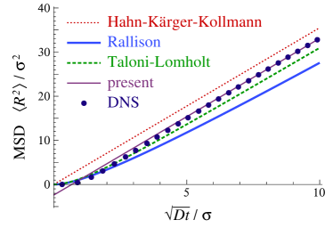
(a) (b)

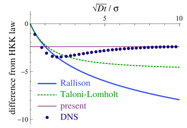
Figure 4: Comparison of the 1D MSD calculated by the HKK law (2.2), Rallison’s equation (3.3), the Taloni–Lomholt solution (3.18), and the present result in Eq. (5.13), with the result of DNS[23] where $N=2^{15}$ and $\rho_{0}=N/L=0.25/\sigma$. (a) The values of MSD, nondimensionalized with $\sigma^{2}$, are plotted against $\sqrt{Dt}/\sigma$. The straight line shows the HKK law, $\left\langle{\smash{R^{2}}}\right\rangle_{\text{HKK}}$, in Eq. (2.2). (b) The difference between the calculated MSD and $\left\langle{\smash{R^{2}}}\right\rangle_{\text{HKK}}$ for each case are plotted in the same way as in (a).

6 2D Colloidal Liquid

Finally we have arrived at the stage where analysis of 2D colloidal liquids is within our reach. The greatest difference in comparison to the 1D case is the presence of the transverse mode.

6.1 Linear analysis of 2D colloidal liquid

Here we target on calculation of both the longitudinal and transverse displacement correlations, namely $X_{\parallel}$ and $X_{\perp}$ in Eq. (4.33), based on linear analysis of the 2D Dean–Kawasaki equation.

The approach is basically in parallel with the 1D case. We start from the Dean–Kawasaki equation, written in the form

$$\mathbf{Q}=-D\,\left(\nabla\rho+\frac{\rho}{{k_{\text{B}}}T}\nabla{U}\right)+\sum_{j}\rho_{j}(\mathbf{r},t)\mathbf{f}_{j}(t)$$ (6.1)

where $U=U[\rho](\mathbf{r})=\int V_{\text{eff}}(r_{*})\rho(\tilde{\mathbf{r}})\mathrm{d}^{2}\tilde{\mathbf{r}}$ with $r_{*}=\left|{\mathbf{r}-\tilde{\mathbf{r}}}\right|$. The thermal noise $\mathbf{f}_{j}(t)$ is subject to Eq. (1.2). Changing the independent variables from $(\mathbf{r},t)$ to $(\bm{\xi},t)$ and taking the field variable $(\Psi_{1},\Psi_{2})$ whose conservation law is given as

$$\ell_{0}\partial_{t}\begin{bmatrix}\Psi_{1}(\bm{\xi},t)\\ \Psi_{2}(\bm{\xi},t)\end{bmatrix}=\begin{bmatrix}\partial_{\xi}{u_{x}(\bm{\xi},t)}\\ \partial_{\eta}{u_{y}(\bm{\xi},t)}\end{bmatrix},$$ (6.2)

we rewrite Eq. (6.1) in the form corresponding to Eq. (5.2):

$$\mathbf{u}=-D\left(\frac{\nabla\rho}{\rho}+\frac{\nabla{U}}{{k_{\text{B}}}T}\right)+\sum_{j}\delta^{2}(\bm{\xi}-\bm{\Xi}_{j})\mathbf{f}_{j}(t),$$ (6.3)

where $\nabla=(\nabla\xi)\partial_{\xi}+(\nabla\eta)\partial_{\eta}$ is expressible in terms of $\Psi_{1}$ and $\Psi_{2}$.

Linear analysis of Eqs. (6.2) and (6.3) is then performed. In terms of the Fourier modes introduced in Eq. (4.23), the linearized equation reads

$$\partial_{t}\begin{bmatrix}\check{\Psi}_{1}(\mathbf{k},t)\\ \check{\Psi}_{2}(\mathbf{k},t)\end{bmatrix}=-D^{\text{c}}_{*}\begin{bmatrix}k_{1}^{2}&k_{1}^{2}\\[2.15277pt] k_{2}^{2}&k_{2}^{2}\end{bmatrix}\begin{bmatrix}\check{\Psi}_{1}(\mathbf{k},t)\\ \check{\Psi}_{2}(\mathbf{k},t)\end{bmatrix}+\ell_{0}^{-1}\begin{bmatrix}\check{f}_{1}(\mathbf{k},t)\\ \check{f}_{2}(\mathbf{k},t)\end{bmatrix},$$ (6.4)

with the forcing statistics given by

$$\ell_{0}^{-2}\begin{bmatrix}\left\langle{{\check{f}_{1}(\mathbf{k},t)}{\check{f}_{1}(-\mathbf{k}^{\prime},t^{\prime})}}\right\rangle&\left\langle{{\check{f}_{1}(\mathbf{k},t)}{\check{f}_{2}(-\mathbf{k}^{\prime},t^{\prime})}}\right\rangle\\ \left\langle{{\check{f}_{2}(\mathbf{k},t)}{\check{f}_{1}(-\mathbf{k}^{\prime},t^{\prime})}}\right\rangle&\left\langle{{\check{f}_{2}(\mathbf{k},t)}{\check{f}_{2}(-\mathbf{k}^{\prime},t^{\prime})}}\right\rangle\end{bmatrix}=\frac{2{D_{*}}}{N}\begin{bmatrix}k_{1}^{2}&0\\ 0&k_{2}^{2}\end{bmatrix}\delta_{\mathbf{k},\mathbf{k}^{\prime}}\delta(t-t^{\prime}),$$ (6.5)

where the delta-correlation in regard to the wavenumber originates from the randomness of the particle configuration; possible correction at shorter length scales is ignored for the present.

The linear part of Eq. (6.4) has two eigenvalues: $k_{1}^{2}+k_{2}^{2}$ and $0$, correspond to the dilatational and rotational modes, respectively. The correlations $C_{\alpha\beta}(\mathbf{k},t,s)$ in Eq. (4.26) are then calculated, according to Eq. (4.31), as linear combinations of ${C}_{\mathrm{d}}={C}_{\mathrm{d}}(\mathbf{k},t,s)$ and ${C}_{\mathrm{r}}={C}_{\mathrm{r}}(\mathbf{k},t,s)$. These correlations are given as

$${C}_{\mathrm{d}}(\mathbf{k},t,s) =\frac{S}{L^{4}}\exp\left[-D^{\text{c}}_{*}\mathbf{k}^{2}(t-s)\right],$$ (6.6a)

$${C}_{\mathrm{r}}(\mathbf{k},t,s) =\frac{2D_{*}\mathbf{k}^{2}}{L^{4}}(s-o),$$ (6.6b)

where $o$ is a constant of integration, interpretable as the time at which ${C}_{\mathrm{r}}$ is reset. Note that both ${C}_{\mathrm{d}}$ and ${C}_{\mathrm{r}}$ are independent of the direction of $\mathbf{k}$.

The last step is to convert ${C}_{\mathrm{d}}$ and ${C}_{\mathrm{r}}$ into the displacement correlation. Using the 2D AP formula in the form of Eq. (4.32) and introducing $\theta^{2}=(\xi^{2}+\eta^{2})/(4{D^{\text{c}}_{*}}t)\simeq\tilde{\mathbf{d}}^{2}/[\lambda(t)]^{2}$ with $\lambda(t)=2\sqrt{{D^{\text{c}}}t}$, we obtain

$$\left\langle{{R_{1}(\bm{\xi},t,s)}{R_{1}(\mathbf{0},t,s)}}\right\rangle=\frac{S}{{4\pi}\rho_{0}}\left[E_{1}(\theta^{2})+\frac{\xi^{2}-\eta^{2}}{\xi^{2}+\eta^{2}}\frac{e^{-\theta^{2}}}{\theta^{2}}\right]$$ (6.7a)

$$\left\langle{{R_{2}(\bm{\xi},t,s)}{R_{2}(\mathbf{0},t,s)}}\right\rangle=\frac{S}{{4\pi}\rho_{0}}\left[E_{1}(\theta^{2})+\frac{-\xi^{2}+\eta^{2}}{\xi^{2}+\eta^{2}}\frac{e^{-\theta^{2}}}{\theta^{2}}\right]$$ (6.7b)

$$\left\langle{{R_{1}(\bm{\xi},t,s)}{R_{2}(\mathbf{0},t,s)}}\right\rangle=\frac{S}{{2\pi}\rho_{0}}\frac{\xi\eta}{\xi^{2}+\eta^{2}}\frac{e^{-\theta^{2}}}{\theta^{2}},$$ (6.7c)

which can be rearranged, in terms of $\phi$ such that $\tilde{\mathbf{d}}=(\tilde{{d}}\,{\cos\phi},\;\tilde{{d}}\,{\sin\phi})$, as

$$\left\langle{{\mathbf{R}(\bm{\xi},t,s)}\otimes{\mathbf{R}(\mathbf{0},t,s)}}\right\rangle=\frac{S}{{4\pi}\rho_{0}}\begin{bmatrix}E_{1}(\theta^{2})+\dfrac{e^{-\theta^{2}}}{\theta^{2}}\cos{2\phi}&\dfrac{e^{-\theta^{2}}}{\theta^{2}}\sin{2\phi}\\ \dfrac{e^{-\theta^{2}}}{\theta^{2}}\sin{2\phi}&E_{1}(\theta^{2})-\dfrac{e^{-\theta^{2}}}{\theta^{2}}\cos{2\phi}\end{bmatrix}.$$ (6.8)

By comparing Eq. (6.8) with Eq. (4.33), on the ground that the expression on the left-hand side of Eq. (6.8) equals $\mathsf{X}$ according to Eq. (4.17), we reach the goal of forming expressions for $X_{\parallel}$ and $X_{\perp}$. For large $\theta$, using the asymptotic form of the exponential integral $E_{1}(\theta^{2})$, we find

$$X_{\parallel}(\xi,t) =\frac{S}{{4\pi}\rho_{0}}\left[E_{1}({\theta^{2}})+\frac{e^{-\theta^{2}}}{\theta^{2}}\right]\simeq\frac{S}{{4\pi}\rho_{0}}e^{-\theta^{2}}\left(2\theta^{-2}-\theta^{-4}+\cdots\right)$$ (6.9a)

$$X_{\perp}(\xi,t) =\frac{S}{{4\pi}\rho_{0}}\left[E_{1}({\theta^{2}})-\frac{e^{-\theta^{2}}}{\theta^{2}}\right]\simeq\frac{S}{{4\pi}\rho_{0}}e^{-\theta^{2}}\left(-\theta^{-4}+\cdots\right).$$ (6.9b)

6.2 Discussion

According to Eq. (6.9a), the longitudinal displacement correlation $X_{\parallel}$ is positive, while the transverse displacement correlation $X_{\perp}$ in Eq. (6.9b) is negative. This is qualitatively consistent with the vortical cooperative motion observed by Doliwa and Heuer[14]. Numerical verification of Eqs. (6.9) will be reported elsewhere[87].

By analogy with the 1D displacement correlation in Eq. (5.7) whose limiting value for $\theta\to 0$ correctly gives the HKK law (2.2) of MSD, one may naturally expect that the 2D displacement correlation in Eqs. (6.9) will provide the MSD in the limit of $\theta\to 0$. Unfortunately, it turns out that the 2D linear theory does not give a quantitatively correct value of the MSD, because it is not accurate enough in the short-wave region. We may still attempt, however, a qualitative estimation of the MSD in terms of $X_{\parallel}$ in Eq. (6.9a). Introducing the nondimensionalized cutoff length $\xi_{\text{cut}}\sim\sigma/\ell_{0}$ and using asymptotic form of the exponential integral for small $\theta$, we may estimate the MSD as

$$\left\langle{\smash{\mathbf{R}^{2}}}\right\rangle\sim X_{\parallel}(\xi_{\text{cut}},t)\sim{O(1)}\times\frac{Dt}{{\rho_{0}}\sigma^{2}}+\frac{O(1)}{\rho_{0}}\log{\frac{Dt}{\sigma^{2}}}.$$ (6.10)

Thus we obtain normal diffusion with a logarithmic correction term. This seems to be qualitatively consistent with the result of van Beijeren and Kutner[59] for 2D lattices. The logarithmic correction seems to have the same physical origin as the MSD for 2D elastic bodies in Eq. (3.28).

Nevertheless, we must emphasize that the validity of Eq. (6.10) is rather limited and, in particular, it is definitely incorrect for dense colloidal systems such as the one depicted in Fig. 3(a). This is not the fault of the AP formula but the limitation of the linear theory, as the time needed for the $\alpha$ relaxation is largely underestimated by ignoring the nonlinear effects of the interacting particles with finite $\sigma$. Evidently, a nonlinear theory for ${C}_{\mathrm{d}}$ and ${C}_{\mathrm{r}}$ should be developed and used instead of Eqs. (6.6). Combination of such nonlinear theory and the AP formula will provide a better estimation of the MSD in 2D systems.

Some insights into the $\alpha$ relaxation may be given by comparative discussion on SFD in quasi-1D systems and 2D dense colloidal liquid. The $\alpha$ relaxation in colloidal liquid is believed to involve cooperation of numerous particles that occurs in some localized yet extended mode, often termed as a cooperatively rearranging region[88]. As a drastic simplification of a cooperatively rearranging region in the spirit of mean-field approximation, we may replace most of the particles with confining walls and consider only two particles explicitly, so that the $\alpha$ relaxation is modeled by the positional exchange of two particles in a quasi-1D channel. Let us denote the position vector of the particles with $\mathbf{r}_{1}=(X_{1},Y_{1})$ and $\mathbf{r}_{2}=(X_{2},Y_{2})$, and the potential with

$$U=U(\mathbf{r}_{1},\mathbf{r}_{2})=V(r_{12})+U_{\text{ex}}(Y_{1})+U_{\text{ex}}(Y_{2})$$ (6.11)

where $V(r_{12})$ is the interaction potential as a function of $r_{12}=\left|{\mathbf{r}_{2}-\mathbf{r}_{1}}\right|$ and $U_{\text{ex}}(Y_{i})$ is the confinement potential for the $i$-th particle. The barrier potential for the positional exchange of $X_{1}$ and $X_{2}$ is given in terms of configurational integral, as

$$V_{\text{1D}}=V_{\text{1D}}(X_{2}-X_{1})=-{k_{\text{B}}}T\log\left(\iint e^{-{\beta}U}\mathrm{d}{Y_{1}}\mathrm{d}{Y_{2}}\right)+\text{const.},$$ (6.12)

where $\beta=1/({k_{\text{B}}}T)$. The “hopping rate” for the positional exchange[43], denoted with $1/\tau_{\text{hop}}$, is proportional to $e^{-\beta\max{V_{\text{1D}}}}$. Let us discuss how $\tau_{\text{hop}}$ depends on $U_{\text{ex}}$, comparing two cases:

$$U_{\text{ex}}(Y_{i}) =U_{\text{soft}}(Y_{i})={\frac{\kappa}{2}}Y_{i}^{2}$$ (6.13a)

and

$$U_{\text{ex}}(Y_{i}) =U_{\text{hard}}(Y_{i})=\begin{cases}0&(\left|{Y_{i}}\right|<L_{y})\\ \infty&(\left|{Y_{i}}\right|>L_{y}).\end{cases}$$ (6.13b)

By assuming $V(r)$ to be rigid sphere potential in both cases for the sake of simplicity, the integral in Eq. (6.12) can be concretely evaluated. In the case of the soft wall in Eq. (6.13a), we find $\log\tau_{\text{hop}}\propto\kappa\sigma^{2}/({k_{\text{B}}}T)$ in the limit of low temperature; this expression of $\tau_{\text{hop}}$ has no singularity as a function of $\kappa$ and $\sigma$. Contrastively, $\tau_{\text{hop}}$ in the hard wall case with Eq. (6.13b) has a singularity as a function of $L_{y}$ and $\sigma$, as it diverges for $\sigma/L_{y}\to 1/2$. Thus we find that the $\sigma$-dependence of $\tau_{\text{hop}}$, or the dependence of $\tau_{\text{hop}}$ on the strength of the wall confinement, can be sharp or blunt depending on whether the wall is rigid or not. This behavior seems to be consistent with the numerical findings of Lucena et al.[41] In the case of 2D and 3D colloidal liquids, the corresponding problem is how the timescale of the $\alpha$ relaxation depends on the volume fraction $\phi$. It is known that this timescale can exhibit an extremely sharp dependence on $\phi$, expressible as $e^{B/(\phi_{0}-\phi)}$ with $B$ and $\phi_{0}$ being some constants[12, 89]; in comparison, the singularity of $\tau_{\text{hop}}$ for $U_{\text{ex}}(Y_{i})=U_{\text{hard}}(Y_{i})$ in the quasi-1D channel is much weaker, as it diverges only algebraically. This difference suggests subtlety of the cooperative dynamics in the $\alpha$ relaxation in colloidal liquids that is difficult to capture by the “mean-field” approach discussed here.

7 Concluding remarks

In search of insight into cooperativity associated with the cage effect in glassy liquids, we have developed a formalism to calculate the displacement correlation tensor, $\left\langle{\mathbf{R}(\bm{\xi},t)\otimes\mathbf{R}(\bm{\xi}^{\prime},t)}\right\rangle$, in ${n_{\text{d}}}$-dimensional systems. The calculation relies on the label variable method, i.e. adoption of the Lagrangian description[22, 23].

In the 1D case, Eq. (4.7) gives the MSD as a special case of the displacement correlation in Eq. (4.10). These equations improve on the original formula (3.19) in that they are asymptotically exact for $N\to\infty$ by virtue of the Lagrangian description. By combining Eq. (4.7) with the Lagrangian MCT equation (5.12), we have calculated a finite-time correction to the asymptotic HKK law (2.2). The formula was also applied to an ageing SFD and reproduced the effect of the initial condition on the MSD, previously obtained by Leibovich and Barkai[55] with a different approach. It will be interesting to study various extensions of SFD with the AP formula (4.7), so that the effect of spatially correlated noise[28] may be clarified, for example.

Our main result is the 2D formula (4.32), which is tensorial. For isotropic systems, the displacement correlation tensor reduces to the longitudinal correlation $X_{\parallel}$ and the transverse correlation $X_{\perp}$. Linear analysis of the two-dimensional colloidal system predicts $X_{\perp}>0$ and $X_{\parallel}<0$, which seems to be qualitatively consistent with the vortical cooperative motion observed in numerical simulations[14].

As a future direction, it is promising to improve the 2D result by introducing nonlinear theory for ${C}_{\mathrm{d}}$ and ${C}_{\mathrm{r}}$, for which Eq. (5.12) provides an encouraging prototype. On the side of SFD, more attention should be paid to cooperativity. In particular, it would be interesting to devise an extension of SFD in which $\alpha$ relaxation occurs cooperatively, as it would shed more light on studies of glassy dynamics than the classical SFD which is essentially $\beta$ relaxation in 1D systems.

References

- [1] A. Taloni and F. Marchesoni, Biophys. Rev. Lett. 9 (2014).
- [2] C. Coste, J.-B. Delfau and M. S. Jean, Biophys. Rev. Lett. 9 (2014).
- [3] A. J. Liu and S. R. Nagel, Jamming and Rheology: Constrained Dynamics on Microscopic and Macroscopic Scales (Taylor & Francis, London, 2001).
- [4] L. Berthier and G. Biroli, Rev. Mod. Phys. 83, 587 (2011).
- [5] S. P. Das, Statistical Physics of Liquids at Freezing and Beyond (Cambridge Univ. Press, 2011).
- [6] F. Höfling and T. Franosch, Rep. Prog. Phys. 76, 046602 (2013).
- [7] R. Yamamoto and A. Onuki, Phys. Rev. E 58, 3515 (1998).
- [8] L. Berthier, G. Biroli, J.-P. Bouchaud, L. Cipelletti and W. van Saarloos (eds.), Dynamical Heterogeneities in Glasses, Colloids, and Granular Media (Oxford University Press, Oxford, 2011).
- [9] W. Götze and L. Sjögren, Transport Theory and Statistical Physics 6-8, 801 (1995).
- [10] W. Kob and H. C. Andersen, Phys. Rev. E 51, 4626 (1995).
- [11] W. Kob and H. C. Andersen, Phys. Rev. E 52, 4134 (1995).
- [12] D. R. Reichman and P. Charbonneau, J. Stat. Mech. , P05013 (2005).
- [13] M. Otsuki and H. Hayakawa, Phys. Rev. E 86, 031505 (2012).
- [14] B. Doliwa and A. Heuer, Phys. Rev. E 61, 6898 (2000).
- [15] C. Brito and M. Wyart, J. Chem. Phys. 131, 024504 (2009).
- [16] S. Sota and M. Itoh, Journal of Korean Physical Society 54, 386 (2009).
- [17] C. Donati, J. F. Douglas, W. Kob, S. J. Plimpton, P. H. Poole and S. C. Glotzer, Phys. Rev. Lett. 80, 2338 (1998).
- [18] C. Dasgupta, A. V. Indrani, S. Ramaswamy and M. K. Phani, Europhys. Lett. 15, 307 (1991).
- [19] S. C. Glotzer, V. N. Novikov and T. B. Schrøder, J. Chem. Phys. 112, 509 (2000).
- [20] H. Shiba, T. Kawasaki and A. Onuki, Phys. Rev. E 86, 041504 (2012).
- [21] T. Kawasaki and A. Onuki, Phys. Rev. E 87, 012312 (2013).
- [22] Ooshida T., S. Goto, T. Matsumoto, A. Nakahara and M. Otsuki, J. Phys. Soc. Japan 80, 074007 (2011).
- [23] Ooshida T., S. Goto, T. Matsumoto, A. Nakahara and M. Otsuki, Phys. Rev. E 88, 062108 (2013).
- [24] S. N. Majumdar and M. Barma, Physica A 177, 366 (1991).
- [25] J. M. Rallison, J. Fluid Mech. 186, 471 (1988).
- [26] H. van Beijeren, K. W. Kehr and R. Kutner, Phys. Rev. B 28, 5711 (1983).
- [27] K. Nelissen, V. Misko and F. Peeters, Europhys. Lett. 80, 56004 (2007).
- [28] D. Tkachenko, V. Misko and F. Peeters, Phys. Rev. E 82, 051102 (2010).
- [29] S. Alexander and P. Pincus, Phys. Rev. B 18, 2011 (1978).
- [30] A. L. Hodgkin and R. D. Keynes, J. Physiol. 128, 61 (1955).
- [31] T. E. Harris, J. Appl. Probab. 2, 323 (1965).
- [32] A. Lefèvre, L. Berthier and R. Stinchcombe, Phys. Rev. E 72, 010301(R) (2005).
- [33] S. M. Abel, Y.-L. S. Tse and H. C. Andersen, Proc. Natl. Acad. Sci. USA 106, 15142 (2009).
- [34] H. Frusawa, Phys. Lett. A 378, 1780 (2014).
- [35] K. Miyazaki and A. Yethiraj, J. Chem. Phys. 117, 10448 (2002).
- [36] P. Pal, C. S. O’Hern, J. Blawzdziewicz, E. R. Dufresne and R. Stinchcombe, Phys. Rev. E 78, 011111 (2008).
- [37] K. Hahn and J. Kärger, J. Phys. A: Math. Gen. 28, 3061 (1995).
- [38] M. Kollmann, Phys. Rev. Lett. 90, 180602 (2003).
- [39] G. Nägele, Physics Reports 272, 215 (1996).
- [40] J. K. G. Dhont, An Introduction to Dynamics of Colloids (Elsevier, Amsterdam, 1996).
- [41] D. Lucena, D. Tkachenko, K. Nelissen, Misko, Ferreira, Farias and Peeters, Phys. Rev. E 85, 031147 (2012).
- [42] U. Siems, C. Kreuter, A. Erbe, N. Schwierz, S. Sengupta, P. Leiderer and P. Nielaba, Scientific Reports 2, 1015 (2012).
- [43] S. N. Wanasundara, R. J. Spiteri and R. K. Bowles, J. Chem. Phys. 140, 024505 (2014).
- [44] Ooshida T., S. Goto, T. Matsumoto and M. Otsuki, Displacement correlation as an indicator of collective motion in one-dimensional and quasi-one-dimensional systems of repulsive Brownian particles, to be published in Mod. Phys. Lett. B.
- [45] O. Flomenbom and A. Taloni, Europhys. Lett. 83, 20004 (2008).
- [46] O. Flomenbom, Phys. Rev. E 82, 031126 (2010).
- [47] O. Flomenbom, Phys. Lett. A 374, 4331 (2010).
- [48] O. Flomenbom, Europhys. Lett. 94, 58001 (2011).
- [49] H. H. Ussing, Acta Physiol. Scand. 19, 43 (1949).
- [50] C.-P. Hsieh, Biophysical Chemistry 139, 57 (2009).
- [51] B. Hille, C. M. Armstrong and R. Mackinnon, Nature Medicine 5, 1105 (1999).
- [52] T. L. Hill and Y.-D. Chen, Proc. Nat. Acad. Sci. USA 68, 1711 (1971).
- [53] E. Barkai and R. Silbey, Phys. Rev. Lett. 102, 050602 (2009).
- [54] E. Barkai and R. Silbey, Phys. Rev. E 81, 041129 (2010).
- [55] N. Leibovich and E. Barkai, Phys. Rev. E 88, 032107 (2013).
- [56] P. N. Pusey and W. van Megen, Phys. Rev. Lett. 59, 2083 (1987).
- [57] A. Taloni and M. A. Lomholt, Phys. Rev. E 78, 051116 (2008).
- [58] R. Kutner, H. van Beijeren and K. W. Kehr, Phys. Rev. B 30, 4382 (1984).
- [59] H. van Beijeren and R. Kutner, Phys. Rev. Lett. 55, 238 (1985).
- [60] M. Sellitto and J. J. Arenzon, Phys. Rev. E 62, 7793 (2000).
- [61] J.-P. Hansen and I. R. McDonald, Theory of Simple Liquids, 3rd edn. (Academic Press, Amsterdam, 2006).
- [62] D. S. Dean, J. Phys. A: Math. Gen. 29, L613 (1996).
- [63] K. Kawasaki, Physica A 208, 35 (1994).
- [64] K. Kawasaki, Journal of Statistical Physics 93, 527 (1998).
- [65] M. H. J. Hagen, I. Pagonabarraga, C. P. Lowe and D. Frenkel, Phys. Rev. Lett. 78, 3785 (1997).
- [66] B. J. Alder and T. E. Wainwright, Phys. Rev. A 1, 18 (1970).
- [67] L. Lizana, T. Ambjörnsson, A. Taloni, E. Barkai and M. A. Lomholt, Phys. Rev. E 81, 051118 (2010).
- [68] W. Götze and L. Sjögren, Rep. Prog. Phys. 55, 241 (1992).
- [69] W. Götze, Complex Dynamics of Glass-Forming Liquids: A Mode-coupling theory (Oxford University Press, New York, 2009).
- [70] P. A. Fedders, Phys. Rev. B 17, 40 (1978).
- [71] P. M. Centres and S. Bustingorry, Phys. Rev. E 81, 061101 (2010).
- [72] M. Doi and S. F. Edwards, The Theory of Polymer Dynamics (Oxford, 1986).
- [73] S. N. Majumdar and M. Barma, Phys. Rev. B 44, 5306 (1991).
- [74] S. F. Edwards and D. R. Wilkinson, Proc. R. Soc. London, Ser. A 381, 17 (1982).
- [75] J. Krug, Adv. in Phys. 46, 139 (1997).
- [76] C. Brito and M. Wyart, Europhys. Lett. 76, 149 (2006).
- [77] C. Toninelli, M. Wyart, L. Berthier, G. Biroli and J.-P. Bouchaud, Phys. Rev. E 71, 041505 (2005).
- [78] B. Jancovici, Phys. Rev. Lett. 19, 20 (1967).
- [79] H. Diamant, Criteria of amorphous solidification, arXiv:1406.2508.
- [80] R. H. Kraichnan, Physics of Fluids 8, 575 (1965).
- [81] Y. Kaneda, J. Fluid Mech. 107, 131 (1981).
- [82] S. Kida and S. Goto, J. Fluid Mech. 345, 307 (1997).
- [83] R. B. Bird, R. C. Armstrong and O. Hassager, Dynamics of polymeric liquids, second edn. (Wiley, New York, 1987).
- [84] R. H. Kraichnan, J. Fluid Mech. 5, 497 (1959).
- [85] S. Goto and S. Kida, Physica D 117, 191 (1998).
- [86] W. Kob and J.-L. Barrat, Phys. Rev. Lett. 78, 4581 (1997).
- [87] Ooshida T., S. Goto, T. Matsumoto and M. Otsuki, Calculation of displacement correlation tensor indicating vortical cooperative motion in two-dimensional colloidal liquids (in preparation).
- [88] G. Adam and J. H. Gibbs, J. Chem. Phys. 43, 139 (1965).
- [89] T. Kawasaki and H. Tanaka, J. Phys.: Condens. Matter 23, 194121 (2011).