Abstract

We consider in this paper a class of semi-continuous quadratic programming problems which arises in many real-world applications such as production planning, portfolio selection and subset selection in regression. We propose a lift-and-convexification approach to derive an equivalent reformulation of the original problem. This lift-and-convexification approach lifts the quadratic term involving $x$ only in the original objective function $f(x,y)$ to a quadratic function of both $x$ and $y$ and convexifies this equivalent objective function. While the continuous relaxation of our new reformulation attains the same tight bound as achieved by the continuous relaxation of the well known perspective reformulation, the new reformulation also retains the linearly constrained quadratic programming structure of the original mix-integer problem. This prominent feature improves the performance of branch-and-bound algorithms by providing the same tightness at the root node as the state-of-the-art perspective reformulation and offering much faster processing time at children nodes. We further combine the lift-and-convexification approach and the quadratic convex reformulation approach in the literature to form an even tighter reformulation. Promising results from our computational tests in both portfolio selection and subset selection problems numerically verify the benefits from these theoretical features of our new reformulations.

1 Introduction

We consider in this paper the following mixed-integer quadratic programming (MIQP) problem:

$$({\rm P})~{}~{}\min ~{}~{}f(x,y)=x^{T}Qx+c^{T}x+h^{T}y$$

$${\rm s.t.} ~{}~{}Ax+By\leq d,$$

$$~{}~{}a_{i}y_{i}\leq x_{i}\leq b_{i}y_{i},~{}y_{i}\in\{0,1\},~{}i=1,\ldots,n,$$ (1)

where $Q$ is an $n\times n$ positive semidefinite symmetric matrix, $c,h\in\Re^{n}$, $d\in\Re^{m}$, and $A,B\in\Re^{m\times n}$.

Problem (P) is in general NP-hard (see bienstock96 ). Its difficulty arises from the discrete structure induced by the constraint in (1). This constraint is used to model the situation where $x_{i}$ must rest inside an interval if it is not zero, that is, $x_{i}\in\{0\}\cup[a_{i},b_{i}]$. These variables $x_{i}$ are termed semi-continuous variables. We assume in our study $a_{i}<b_{i},~{}i=1,...,n$. We also assume that the feasible region of problem (P) is nonempty. A recent review on problem (P) and its solution methods can be found in sun2013 .

Semi-continuous variables appear in many real-world optimization problems. For instance, in production planning, the semi-continuous variables are used to describe the state of a production process that is either turned off (inactive), hence nothing is produced, or turned on (active) such that the production level has to lie in certain interval (frangioni2006or , frangioni2008power , frangioni2009ieee ). Other typical applications of semi-continuous variables include portfolio selection with minimum buy-in threshold (jobst01 , frangioni06mp , cui2013 , sun2013 ) and lot-sizing with minimum order quantity (anderson1993 , park2013lot ).

An important instance of (P) involves optimization models with a cardinality constraint:

$$|{\rm supp}(x)|\leq K,$$ (2)

where ${\rm supp}(x)=\{i~{}|~{}x_{i}\neq 0\}$ and $K$ is an integer with $1\leq K\leq n$. The cardinality constraint is often encountered when the number of nonzero variables has to be limited. The cardinality constraint in (2) can be easily incorporated into problem (P) by introducing an additional linear constraint $\sum_{i=1}^{m}y_{i}\leq K$.

A well-known application of semi-continuous variables and cardinality constraint is the cardinality constrained mean-variance portfolio selection in financial optimization. The classical mean-variance model of Markowitz is a quadratic programming problem that minimizes the variance subject to linear constraints on expected return and budget availabilities. In real-world applications of portfolio selection models, however, most investors would invest in only a limited number of assets due to market frictions such as management and transaction fees. Moreover, the minimum buy-in threshold is often a mandate trading constraint. Suppose that there are $n$ risky assets in a financial market with a random return vector $R=(R_{1},\ldots,R_{n})^{T}$. Furthermore, the expected return vector and the covariance matrix of $R$ are assumed to be given as $\mu$ and $Q$, respectively. The portfolio selection model with cardinality and minimum buy-in threshold constraints can be then expressed as:

$${\rm(MV)}~{}~{}\min ~{}~{}x^{T}Qx$$

$${\rm s.t.} ~{}~{}\sum^{n}_{i=1}x_{i}=1,$$

$$~{}~{}\mu^{T}x\geq\rho,$$

$$~{}~{}\sum_{i=1}^{n}y_{i}\leq K,$$

$$~{}~{}a_{i}y_{i}\leq x_{i}\leq b_{i}y_{i},~{}y_{i}\in\{0,1\},~{}i=1,\ldots,n,$$

where $x_{i}$ represents the proportion of the total capital invested in the $i$th asset, and $\rho$ is a prescribed expected return level set by the investor. Portfolio selection problems with cardinality and/or minimum threshold constraints have been studied extensively in recent literature. For exact solution methods, please see, e.g., bienstock96 , li06 , shawa08 , bonami09 , bertsimas09 , cui2013 , gaoli2013b . For inexact solution methods, such as heuristics, local search methods and randomized techniques, please see, e.g., jacob74 , blog83 , chang00 , jobst01 , schaerf02 , maringer03 , crama03 , mitra07 , fernandez07 , zhang08 .

Another application of (P) with cardinality constraint is the subset selection problem in multivariate linear regression. Given $m$ observed data points $(a_{i},b_{i})$ with $a_{i}\in\Re^{n}$ and $b_{i}\in\Re$, we need to minimize the least square measure of $\sum_{i=1}^{m}(a_{i}^{T}x-b_{i})^{2}$ with only a subset of the prediction variables in $x$ (see, e.g., arthanari93 , miller02 , bertsimas09 ). This problem can be formally formulated as:

$${\rm(SSP)}~{}~{}\min ~{}~{}\|Ax-b\|^{2}$$

$${\rm s.t.} ~{}~{}|{\rm supp}(x)|\leq K,$$

where $A^{T}=(a_{1},\ldots,a_{m})$, $b=(b_{1},\ldots,b_{m})^{T}$, and $K$ is an integer with $1\leq K\leq n$. When we convert this problem to problem (P), lower bounds and upper bounds on $x$, i.e. $L\leq x_{i}\leq U$, can be imposed for a sufficiently large positive number $U$ and a sufficiently small negative number $L$.

Cardinality constrained linear-quadratic optimal control was investigated in GaoLi2011 . Furthermore, a polynomially solvable case of the cardinality-constrained quadratic optimization problem was identified in gaoli2013a .

We focus in this paper on exact solution methods for problem (P). Standard MIQP solvers that are based on branch-and-bound frameworks can be applied to (P) directly. However, the lower bound generated from the continuous relaxation of (P) by relaxing $y_{i}\in\{0,1\}$ to $y_{i}\in[0,1]$ is often quite loose. Equivalent reformulations with tighter continuous relaxation, i.e., a larger lower bound, have been proposed in the literature frangioni06mp , frangioni2007letter , frangioni2009letter , zheng2013 . These reformulations are more efficient when solved in MIQP solvers. We propose a lift-and-convexification approach to construct a tight reformulation for problem (P). This lift-and-convexification approach lifts the quadratic term involving $x$ only in the original objective function $f(x,y)$ to a quadratic function of both $x$ and $y$ and convexifies this equivalent objective function in a quadratic form of $(x,y)$. The new reformulation retains the linearly constrained structure of the MIQP form so that its continuous relaxations can be solved efficiently. At the same time, the lower bound achieved by the continuous relaxation of this newly proposed reformulation is the same as the lower bound obtained from the state-of-the-art perspective reformulation. Thus it improves the performance of branch-and-bound algorithms by providing the same tightness at the root node as the state-of-the-art perspective reformulation and much faster processing time at children nodes. We then further combine our lift-and-convexification approach and the quadratic convex reformulation (QCR) billionnet2008 , billionnet2009qcr approach in the literature to form an even tighter reformulation. The QCR approach has been applied to zero-one quadratic programs billionnet2009qcr and integer quadratic programs billionnet2012qcrExtended . While the QCR approach cannot be directly applied to problem (P), it can be successfully applied on top of our new lift-and-convexification reformulation. This further reduces the duality gap as we will show in our numerical tests.

The paper is organized as follows: In §2, we review the current state-of-the-art reformulation and exact solution methods for problem (P). In §3, we propose a lift-and-convexification approach to obtain a tight reformulation. We show that this new reformulation is as tight as the state-of-the-art reformulation in terms of the lower bound from its continuous relaxation. As the continuous relaxation of the new reformulation is a quadratic program, it can be thus solved efficiently. In §4, we conduct numerical experiments to demonstrate the effectiveness of our new lift-and-convexification reformulation. In §5, we review the QCR approach in the literature for the binary and integer quadratic programs. We then combine lift-and-convexification approach and the QCR approach to form an even tighter reformulation. We conclude our paper in §6.

Notation: Throughout this paper, we denote by $v(\cdot)$ the optimal value of problem $(\cdot)$, and $\Re^{n}_{+}$ the nonnegative orthant of $\Re^{n}$. For any $a\in\Re^{n}$, we denote by ${\rm diag}(a)={\rm diag}(a_{1},\ldots,a_{n})$ the diagonal matrix with $a_{i}$ being its $i$th diagonal element. We denote by $e$ the all-one vector.

2 Literature review and related work

One efficient solution method for (P) is the perspective reformulation proposed by frangioni06mp , frangioni2007letter , in which problem (P) is transformed into the following equivalent form:

$$({\rm PR}(\rho))~{}~{}\min ~{}~{}f_{\rho}(x,y)=x^{T}(Q-{\rm diag}(\rho))x+c^{T}x+h^{T}y+\sum^{n}_{i=1}[\rho_{i}(x^{2}_{i}/y_{i})]$$

$${\rm s.t.} ~{}~{}Ax+By\leq d,$$

$$~{}~{}a_{i}y_{i}\leq x_{i}\leq b_{i}y_{i},~{}y_{i}\in\{0,1\},~{}i=1,\ldots,n,$$

where $\rho\in\Re^{n}$ is chosen such that

$$\rho\geq 0~{}{\rm and}~{}Q-{\rm diag}(\rho)\succeq 0,$$

with an assumption $0/0=0$.

The perspective reformulation is very tight, i.e., the lower bound generated from the continuous relaxation of this reformulation is usually much higher than the lower bound generated directly from the continuous relaxation of (P). To deal with the fractional terms in the objective function of $({\rm PR}(\rho))$, two tractable reformulations of $({\rm PR}(\rho))$ were proposed in the literature.

The first reformulation is a second-order cone programming (SOCP) reformulation akturk2009strong , gunluk2010perspective . For each $i$, introducing an additional variable $\phi_{i}=x_{i}^{2}/y_{i}$ and then rewriting the constraint $\phi_{i}\geq x_{i}^{2}/y_{i}$ as an SOCP constraint yields the following SOCP reformulation:

$$({\rm SOCP}(\rho))~{}~{}\min ~{}~{}x^{T}(Q-{\rm diag}(\rho))x+c^{T}x+h^{T}y+\rho^{T}\phi$$

$${\rm s.t.} ~{}~{}Ax+By\leq d,$$

$$~{}~{}a_{i}y_{i}\leq x_{i}\leq b_{i}y_{i},~{}y_{i}\in\{0,1\},~{}i=1,\ldots,n,$$

$$~{}\left\|\begin{array}[]{c}x_{i}\\ \frac{\phi_{i}-y_{i}}{2}\\ \end{array}\right\|\leq\frac{\phi_{i}+y_{i}}{2},~{}i=1,\ldots,n.$$

However, as the problem size grows, the time needed to solve the above SOCP relaxation becomes a critical factor. When interior point methods are used, the corresponding branch-and-bound algorithm may converge very slowly.

The second reformulation is the perspective cut (PC) reformulation frangioni06mp , frangioni2007letter . Representing the value of $x_{i}^{2}/y_{i}$ by the supremum of a set of infinitely many hyperplanes, which are called perspective cuts, gives rise to the following PC reformulation:

$$({\rm PC}(\rho))~{}~{}\min ~{}~{}x^{T}(Q-{\rm diag}(\rho))x+c^{T}x+h^{T}y+\rho^{T}\phi$$

$${\rm s.t.} ~{}~{}Ax+By\leq d,$$

$$~{}~{}a_{i}y_{i}\leq x_{i}\leq b_{i}y_{i},~{}y_{i}\in\{0,1\},~{}i=1,\ldots,n,$$

$$~{}~{}\phi_{i}\geq 2\overline{x}_{i}x_{i}-\overline{x}_{i}^{2}y_{i},\forall\overline{x}_{i}\in[a_{i},b_{i}],~{}i=1,\ldots,n.$$ (3)

The perspective cuts in (3) can be added dynamically when ${\rm(PC(\rho))}$ is solved in a branch-and-cut framework (see frangioni2009letter ). With the help of warm start and dual methods, quadratic programming relaxations in the perspective cut algorithm can be solved efficiently.

Let $({\rm\overline{PR}}(\rho))$, $({\rm\overline{SOCP}}(\rho))$ and $({\rm\overline{PC}}(\rho))$ denote the continuous relaxations of
$({\rm PR}(\rho))$, $({\rm SOCP}(\rho))$ and $({\rm PC}(\rho))$, respectively, by relaxing $y_{i}\in\{0,1\}$ to $y_{i}\in[0,1]$. It is easy to see that the objective values of these continuous relaxations form the same lower bound for $({\rm P})$. A key issue is how to choose the vector $\rho$ such that this lower bound is as large as possible. One natural way is to set every component of $\rho$ to be the smallest eigenvalue of $Q$. Frangioni and Gentile frangioni2007letter proposed a better heuristic and set $\rho$ to be the optimal solution to the following SDP problem:

$$\max\{e^{T}\rho\mid\rho\geq 0,Q-{\rm diag}(\rho)\succeq 0\}.$$ (4)

Ideally, the best parameter $\rho$ that maximizes the lower bound $v({\rm\overline{PR}}(\rho))$ can be found by solving the following problem:

$$({\rm MAX}\rho)~{}~{}\max\{v({\rm\overline{PR}}(\rho))\mid\rho\geq 0,Q-{\rm diag}(\rho)\succeq 0\}.$$ (5)

Recently, Zheng et al. zheng2013 established the following interesting result.

Theorem 1

Problem $({\rm MAX}\rho)$ is equivalent to the following semi-definite programming (SDP) problem:

$$({\rm SDP}_{l})~{}~{}\max ~{}~{}\tau$$

$${\rm s.t.} ~{}\left(\begin{array}[]{cc}\rho_{i}+\mu_{i}&\frac{1}{2}(c_{i}-\lambda_{i}-(a_{i}+b_{i})\mu_{i})\\ \frac{1}{2}(c_{i}-\lambda_{i}-(a_{i}+b_{i})\mu_{i})^{T}&h_{i}-\pi_{i}+(B^{T}\eta)_{i}+\mu a_{i}bi\end{array}\right)\succeq 0,$$ (8)

$$~{}~{}i=1,\ldots,n,$$

$$~{}\left(\begin{array}[]{cc}Q-{\rm diag}(\rho)&\frac{1}{2}(\lambda+A^{T}\eta)\\ \frac{1}{2}(\lambda+A^{T}\eta)^{T}&-\eta^{T}d-e^{T}\pi-\tau\end{array}\right)\succeq 0,$$ (11)

$$~{}~{}(\eta,\mu,\pi,\rho)\in\Re^{m}_{+}\times\Re^{n}_{+}\times\Re^{n}_{+}\times\Re^{n}_{+},$$

$$~{}~{}(\lambda,\tau)\in\Re^{n}\times\Re.$$

Zheng et al. zheng2013 showed that the perspective cut approach for $({\rm PC}(\rho^{*}))$ with $\rho^{*}$ obtained from $({\rm SDP}_{l})$ is most efficient for solving problem (P) to its optimality.

When $B\equiv 0$ in the constraint $Ax+By\leq d$, Frangioni et al. frangioni2011or developed an equivalent MIQP reformulation of $({\rm PR}(\rho))$, whose continuous relaxation becomes a quadratic programming problem. Frangioni et al. frangioni2013 also proposed an MIQP reformulation of the original problem (P). But the continuous relaxation of this MIQP reformulation is in general not as tight as that of the perspective reformulation.

3 Lift-and-convexification approach

In this section, we derive a tight
MIQP reformulation of (P) by proposing a lift-and-convexification approach. This approach lifts the quadratic term involving $x$ only in the original objective function $f(x,y)$ to an equivalent quadratic function of both $x$ and $y$ and convexifies this equivalent objective function in a quadratic form of $(x,y)$.

Contrast to the the perspective reformulation which involves fractional terms, our new reformulation is a quadratic programming problem whose continuous relaxations can be solved efficiently. At the same time, the lower bound achieved by the continuous relaxation of this new reformulation can be proved to achieve the same lower bound obtained from $({\rm\overline{SOCP}}(\rho^{*}))$ or ${\rm(\overline{PC}(\rho^{*}))}$ with $\rho^{*}$ calculated from $({\rm SDP}_{l})$. To construct the new reformulation, we only need to solve an additional SOCP problem, given the solution for $({\rm SDP}_{l})$.

Let us determine first what kind of quadratic functions in the $(x,y)$-space we need to add to achieve the above mentioned goals.

Theorem 2

Let $q(x,y)$ be a quadratic function of $x$ and $y$. If $q(x,y)=0$ for all $(x,y)\in\{(x,y)\mid a_{i}y_{i}\leq x_{i}\leq b_{i}y_{i}$, $y_{i}\in\{0,1\}$, $i=1,\ldots,n\}$, where $a_{i}<b_{i},~{}i=1,~{}\ldots,~{}n$, then $q(x,y)$ must take the following form:

$$q(x,y)=\sum_{i=1}^{n}q_{i}(x_{i},y_{i}),$$ (12)

where

$$q_{i}(x_{i},y_{i})=u_{i}x_{i}y_{i}+v_{i}y_{i}^{2}-u_{i}x_{i}-v_{i}y_{i}$$ (13)

is a quadratic function of $(x_{i},y_{i})$ parameterized by $(u_{i},v_{i}).$

Proof. If $(x,y)\in\{(x,y)\mid a_{i}y_{i}\leq x_{i}\leq b_{i}y_{i}$, $y_{i}\in\{0,1\}$, $i=1,\ldots,n\}$, then for any $i=1,..,n$, if $y_{i}=0$, then $x_{i}$ must be $0$.

Let $q(x,y)$ be of the following general form:

$$q(x,y)=(x^{T},y^{T})\left(\begin{array}[]{cc}P&F\\ F^{T}&G\\ \end{array}\right)\left(\begin{array}[]{c}x\\ y\\ \end{array}\right)+p^{T}x+g^{T}y,$$

parameterized by $(P,F,G,p,g)\in\mathbb{S}^{n}\times\Re^{n\times n}\times\mathbb{S}^{n}\times\Re^{n}\times\Re^{n}$. Let $x^{i}$ be a vector with a non-zero component only in its $i$th position and $y^{i}$ be a vector with a non-zero component (which is set at one) only in its $i$th position. It is clear that $(x^{i},y^{i})\in\{(x,y)\mid a_{i}y_{i}\leq x_{i}\leq b_{i}y_{i}$, $y_{i}\in\{0,1\}$, $i=1,\ldots,n\}$. If $q(x,y)=0$ for all $(x,y)\in\{(x,y)\mid a_{i}y_{i}\leq x_{i}\leq b_{i}y_{i}$, $y_{i}\in\{0,1\}$, $i=1,\ldots,n\},$ then

$$q(x^{i},y^{i}) =0,$$ (14)

$$q(x^{i}+x^{j},y^{i}+y^{j}) =0,$$ (15)

for any $i,j=1,..,n$. (14) implies

$$P_{ii}x_{i}^{2}+2F_{ii}x_{i}+G_{ii}+p_{i}x_{i}+g_{i}=0.$$ (16)

Because (16) must hold for any $x_{i}\in[a_{i},b_{i}]$ and $a_{i}<b_{i}$, we have

$$P_{ii} =0,$$ (17)

$$2F_{ii} =-p_{i},$$ (18)

$$G_{ii} =-g_{i}.$$ (19)

Furthermore, (15) leads to

$$P_{ii}x_{i}^{2}+2P_{ij}x_{i}x_{j}+P_{jj}x_{j}^{2}+2((F_{ii}+F_{ij})x_{i}+(F_{jj}+F_{ji})x_{j})$$

$$+G_{ii}+2G_{ij}+G_{jj}+p_{i}x_{i}+p_{j}x_{j}+g_{i}+g_{j}=0,$$

which can be simplified to the following equality by using (17)-(19),

$$P_{ij}x_{i}x_{j}+F_{ij}x_{i}+F_{ji}x_{j}+G_{ij}=0.$$

As the above equality holds for any $(x_{i},x_{j})\in[a_{i},b_{i}]\times[a_{j},b_{j}]$ with $a_{i}<b_{i}$ and $a_{j}<b_{j}$, we must have $0=P_{ij}=F_{ij}=F_{ji}=G_{ij}.$ Combining the above equality with (17)-(19) yields the following form of $q(x,y)$,

$$q(x,y)=\sum_{i=1}^{n}2F_{ii}x_{i}y_{i}+G_{ii}y_{i}^{2}-2F_{ii}x_{i}-G_{ii}y_{i},$$

which is of the same form as (13). $\Box$

We propose the following reformulation of (P):

$$({\rm P}(u,v))~{}~{}\min ~{}~{}f_{u,v}(x,y)=f(x,y)+\sum_{i=1}^{n}q_{i}(x_{i},y_{i})$$

$$s.t. ~{}~{}Ax+By\leq d,$$

$$~{}~{}a_{i}y_{i}\leq x_{i}\leq b_{i}y_{i},~{}y_{i}\in\{0,1\},~{}i=1,\ldots,n,$$

where $q_{i}(x_{i},y_{i})$ is defined in (13). It is easy to see that problem $({\rm P}(u,v))$ is equivalent to (P) and the continuous relaxation of $({\rm P}(u,v))$ is a quadratic program.

The difference among equivalent formulations (P), $({\rm PR}(\rho))$, and $({\rm P}(u,v))$ lies in their objective functions. The following example shows the relative relationship among these three objective functions.

Example 1

Consider a univariate function $f(x)=x^{2}-4x$, where $(x,y)\in\Omega=\{(x,y)\mid y\leq x\leq 3y,~{}y\in[0,1]\}$. Let $q(x,y)=-xy+y^{2}+x-y$. Then, $q(x,y)$ is zero at the region $\{(x,y)\mid y\leq x\leq 3y,~{}y\in\{0,1\}\}$. Figure 1 illustrates the original function $f(x)$, the lifted quadratic function $f_{u,v}(x,y):=f(x)+q(x,y)$ and the perspective function $f_{p}(x,y)=\frac{x^{2}}{y}-4x$. While the three functions has the same value when $y\in\{0,1\}$, we can see that $f_{u,v}(x,y)$ always lies between $f(x)$ and $f_{p}(x,y)$ in the region $\Omega$. This can be numerically verified since $f_{u,v}(x,y)-f(x)=(x-y)(1-y)\geq 0$ for all $(x,y)\in\{(x,y)\mid y\leq x\leq 3y,~{}y\in[0,1]\}$. We can also verify that $f_{p}(x,y)-f_{u,v}(x,y)=(1-y)y(x^{2}+y^{2}-xy)\geq 0$ for all $(x,y)\in\{(x,y)\mid y\leq x\leq 3y,~{}y\in(0,1]\}$.

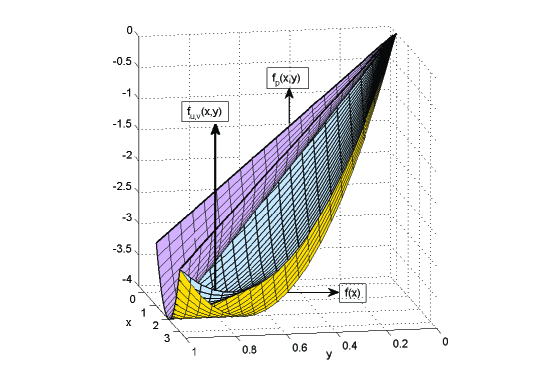
Figure 1: Illustration of the lifting function

Example 1 shows that the objective function of our new reformulation could lie below that of the perspective reformulation. This indicates that our new reformulation may not attain a lower bound that is tighter than the perspective reformulation. However, we will show that our new reformulation can achieve the same lower bound as the perspective reformulation.

Let $u=(u_{1},...,u_{n})^{T}$ and $v=(v_{1},...,v_{n})^{T}$. Now, one critical question is “What is the best parameter vector of $(u,v)$?” Let $({\rm\overline{P}}(u,v))$ denote the continuous relaxation of $({\rm P}(u,v))$ by relaxing $y_{i}\in\{0,1\}$ to $y_{i}\in[0,1]$. It is desirable to choose $(u,v)$ such that the continuous relaxation of $({\rm P}(u,v))$ is as tight as possible. This clear goal motivates us to consider the following problem:

$$({\rm MAX}uv)~{}~{}\max\{v({\rm\overline{P}}(u,v))\mid u,v\in\Re^{n},~{}f_{u,v}(x,y)~{}is~{}convex\}.$$ (20)

Theorem 3

Problem $({\rm MAX}uv)$ is equivalent to the following SDP problem:

$$({\rm SDP}_{q})~{}~{}\max ~{}~{}\tau$$

$${\rm s.t.} ~{}\left(\begin{array}[]{ccc}Q&\frac{1}{2}{\rm diag}(u)&\frac{1}{2}\alpha(u,\eta,\mu,\sigma)\\ \frac{1}{2}{\rm diag}(u)&{\rm diag}(v)&\frac{1}{2}\beta(v,\eta,\mu,\sigma,\lambda,\pi)\\ \frac{1}{2}\alpha(u,\eta,\mu,\sigma)^{T}&\frac{1}{2}\beta(v,\eta,\mu,\sigma,\lambda,\pi)^{T}&-\eta^{T}d-e^{T}\pi-\tau\\ \end{array}\right)\succeq 0,$$ (24)

$$~{}~{}(\eta,\mu,\sigma,\lambda,\pi)\in\Re^{m}_{+}\times\Re^{n}_{+}\times\Re^{n}_{+}\times\Re^{n}_{+}\times\Re^{n}_{+},$$ (25)

$$~{}~{}(u,v,\tau)\in\Re^{n}\times\Re^{n}\times\Re,$$

where

$$\alpha(u,\eta,\mu,\sigma) =c-u+A^{T}\eta-\mu+\sigma,$$ (26)

$$\beta(v,\eta,\mu,\sigma,\lambda,\pi) =h-v+B^{T}\eta+{\rm diag}(a)\mu-{\rm diag}(b)\sigma-\lambda+\pi.$$ (27)

Proof. We first express $({\rm\overline{P}}(u,v))$ by its dual form. Associate the following multipliers to the constraints in $({\rm\overline{P}}(u,v))$:

• $\eta\in\Re^{m}_{+}$ for $Ax+By\leq d$;

• $\mu_{i}$ and $\sigma_{i}\in\Re_{+}$ for $a_{i}y_{i}\leq x_{i}$ and $x_{i}\leq b_{i}y_{i}$, respectively, $i=1,\ldots,n$; and

• $\lambda_{i}$ and $\pi_{i}\in\Re_{+}$ for $y_{i}\geq 0$ and $y_{i}\leq 1$, respectively, $i=1,\ldots,n$.

Let $\mu=(\mu_{1},\ldots,\mu_{n})^{T}$, $\sigma=(\sigma_{1},\ldots,\sigma_{n})^{T}$, $\lambda=(\lambda_{1},\ldots,\lambda_{n})^{T}$ and $\pi=(\pi_{1},\ldots,\pi_{n})^{T}$. Let $\omega$ denote the vector formed by $\eta,\mu,\sigma,\lambda$ and $\pi$. The Lagrangian function of $({\rm\overline{P}}(u,v))$ is then given by

$$L(x,y,\omega) =x^{T}Qx+c^{T}x+h^{T}y+\sum_{i=1}^{n}(u_{i}x_{i}y_{i}+v_{i}y_{i}^{2}-u_{i}x_{i}-v_{i}y_{i})$$

$$~{}~{}~{}+\eta^{T}(Ax+By-d)+\sum_{i=1}^{n}\mu_{i}(a_{i}y_{i}-x_{i})+\sum_{i=1}^{n}\sigma_{i}(x_{i}-b_{i}y_{i})$$

$$~{}~{}~{}+\sum_{i=1}^{n}\lambda_{i}(-y_{i})+\sum_{i=1}^{n}\pi_{i}(y_{i}-1)$$

$$=(x^{T},y^{T})\left(\begin{array}[]{cc}Q&\frac{1}{2}{\rm diag}(u)\\ \frac{1}{2}{\rm diag}(u)&{\rm diag}(v)\\ \end{array}\right)\left(\begin{array}[]{c}x\\ y\\ \end{array}\right)+(c-u+A^{T}\eta-\mu+\sigma)^{T}x$$

$$~{}~{}~{}+(h-v+B^{T}\eta+{\rm diag}(a)\mu-{\rm diag}(b)\sigma-\lambda+\pi)^{T}y-\eta^{T}d-e^{T}\pi.$$

Furthermore, the Lagrangian dual problem of $({\rm\overline{P}}(u,v))$ can be expressed as

$$\max\{\min_{(x,y)\in\Re^{n}\times\Re^{n}}~{}L(x,y,\omega)\mid\omega\geq 0\}.$$ (28)

Introducing an additional variable $\tau$, we can rewrite (28) as

$$\max ~{}~{}\tau$$ (29)

$${\rm s.t.} ~{}~{}\min_{(x,y)\in\Re^{n}\times\Re^{n}}~{}L(x,y,\omega)\geq\tau,$$ (30)

$$~{}~{}\omega\geq 0.$$ (31)

We see that the constraint in (30) is equivalent to $L(x,y,\omega)-\tau\geq 0$ for all $x,y$, which is further equivalent to

$$L(x/t,y/t,\omega)-\tau\geq 0,~{}~{}\forall(x,y)\in\Re^{n}\times\Re^{n},~{}\forall t\in\Re,~{}t\not=0.$$ (32)

Multiplying both sides of (32) by $t^{2}$ yields a homogeneous quadratic form of $(x,y,t)$ in the left-hand side of (32). Thus, the constraint in (30) is equivalent to the following semidefinite constraint:

$$\left(\begin{array}[]{ccc}Q&\frac{1}{2}{\rm diag}(u)&\frac{1}{2}\alpha(u,\eta,\mu,\sigma)\\ \frac{1}{2}{\rm diag}(u)&{\rm diag}(v)&\frac{1}{2}\beta(v,\eta,\mu,\sigma,\lambda,\pi)\\ \frac{1}{2}\alpha(u,\eta,\mu,\sigma)^{T}&\frac{1}{2}\beta(v,\eta,\mu,\sigma,\lambda,\pi)^{T}&-\eta^{T}d-e^{T}\pi-\tau\\ \end{array}\right)\succeq 0,$$ (36)

where $\alpha(u,\eta,\mu,\sigma)$ and $\beta(v,\eta,\mu,\sigma,\lambda,\pi)$ are defined by (26) and (27), respectively. Consequently, the problem in (29)-(31) can be expressed as

$$\max\{\tau\mid{\rm constraint}~{}(\ref{ds31}),~{}\omega\geq 0\}.$$ (37)

If $f_{u,v}(x,y)$ is convex, by the strong duality of convex quadratic programming (see, e.g., Proposition 6.5.6 in bertsekas2003 ), the optimal values of $({\rm\overline{P}}(u,v))$ and (37) are equal. Thus, we have shown that problem $({\rm MAX}uv)$ is equivalent to an SDP problem in the form of $({\rm SDP}_{q})$. $\Box$

Let $(u^{*},v^{*})$ be the optimal parameters for our new reformulation $({\rm P}(u,v))$ by solving the SDP program $({\rm SDP}_{q})$. Let $\rho^{*}$ be the optimal parameters for $({\rm PR}(\rho))$ by solving the SDP program $({\rm SDP}_{l})$. It is necessary to compare the tightness of $v({\rm\overline{P}}(u^{*},v^{*}))$ and $v({\rm\overline{PR}}(\rho^{*}))$, i.e., the bounds from the continuous relaxation of the “best” reformulation proposed in this paper and the “best” perspective reformulation. We will show in the following that these two bounds are the same using constructive proofs.

Theorem 4

Define $\overline{\rho}\in\Re^{n}$ as

$$\overline{\rho}_{i} =\begin{cases}0&{\rm~{}if~{}}v^{*}_{i}=0,\\ \frac{u^{*2}_{i}}{4v^{*}_{i}}&{\rm~{}otherwise},\\ \end{cases}~{}~{}i=1,\ldots,n.$$ (38)

Then,

(a)

$\overline{\rho}$ is feasible for problem $({\rm MAX}\rho)$,

(b)

$v({\rm\overline{P}}(u^{*},v^{*}))\leq v({\rm\overline{PR}}(\overline{\rho}))$.

Proof. (a) From the proof of Theorem 3, we know that there exists $(\tau^{*},\eta^{*},\mu^{*},\sigma^{*},$
$\lambda^{*},\pi^{*})$ such that $(u^{*},v^{*},\tau^{*},\eta^{*},\mu^{*},\sigma^{*},\lambda^{*},\pi^{*})$ is optimal to $({\rm SDP}_{q})$. The constraint in (24) implies that

$$\left(\begin{array}[]{cc}Q&\frac{1}{2}{\rm diag}(u^{*})\\ \frac{1}{2}{\rm diag}(u^{*})&{\rm diag}(v^{*})\\ \end{array}\right)\succeq 0.$$

For any $g\in\Re^{n}$, we define $p\in\Re^{n}$ with

$$p_{i} =\begin{cases}0&{\rm~{}if~{}}v^{*}_{i}=0,\\ -\frac{u^{*}_{i}}{2v^{*}_{i}}g_{i}&{\rm~{}otherwise},\\ \end{cases}~{}~{}i=1,\ldots,n.$$

We then have

$$g^{T}(Q-\overline{\rho})g =g^{T}Qg+\sum^{n}_{i=1}[g_{i}^{2}(-\overline{\rho}_{i})]$$

$$=g^{T}Qg+\sum^{n}_{i=1}[u^{*}_{i}g_{i}p_{i}+v^{*}_{i}p_{i}^{2}]$$

$$=g^{T}Qg+g^{T}{\rm diag}(u^{*})p+p^{T}{\rm diag}(v^{*})p$$

$$=(g^{T},p^{T})\left(\begin{array}[]{cc}Q&\frac{1}{2}{\rm diag}(u^{*})\\ \frac{1}{2}{\rm diag}(u^{*})&{\rm diag}(v^{*})\\ \end{array}\right)\left(\begin{array}[]{c}g\\ p\\ \end{array}\right)$$

$$\geq 0.$$

Hence $(Q-\overline{\rho})\succeq 0$ and $\overline{\rho}$ is feasible to problem $({\rm MAX}\rho)$.

(b) As $({\rm\overline{PR}}(\overline{\rho}))$ and $({\rm\overline{P}}(u^{*},v^{*}))$ have the same feasible region, for any feasible $(x,y)$, we can compare their objective values as follows,

$$f_{\rho}(x,y;~{}\overline{\rho})-f_{u,v}(x,y;~{}u^{*},v^{*})$$ (39)

$$=\sum^{n}_{i=1}[\overline{\rho}_{i}(\frac{x^{2}_{i}}{y_{i}})-\overline{\rho}_{i}x^{2}_{i}-(u^{*}_{i}x_{i}y_{i}+v^{*}_{i}y_{i}^{2}-u^{*}_{i}x_{i}-v^{*}_{i}y_{i})]$$

$$=\sum^{n}_{i=1}[\frac{1}{4v^{*}_{i}}(u_{i}^{*2}x_{i}^{2}\frac{1-y_{i}}{y_{i}}+4u_{i}^{*}v_{i}^{*}x_{i}(1-y_{i})+4v_{i}^{*2}y_{i}(1-y_{i}))]$$

$$=\sum^{n}_{i=1}[\frac{y_{i}(1-y_{i})}{4v^{*}_{i}}((\frac{u_{i}^{*}x_{i}}{y_{i}})^{2}+4u_{i}^{*}v_{i}^{*}\frac{x_{i}}{y_{i}}+4v_{i}^{*2})]$$

$$=\sum^{n}_{i=1}[\frac{y_{i}(1-y_{i})}{4v^{*}_{i}}(u^{*}_{i}\frac{x_{i}}{y_{i}}+2v^{*}_{i})^{2}]$$

$$\geq 0.$$

The above deduction is valid because if $v^{*}_{i}=0$, then $u^{*}_{i}=0$ due to (24). Thus $v({\rm\overline{P}}(u^{*},v^{*}))\leq v({\rm\overline{PR}}(\overline{\rho}))$. $\Box$

The following corollary is a direct result of Theorem 4.

Corollary 1

$v({\rm\overline{P}}(u^{*},v^{*}))\leq v({\rm\overline{PR}}(\rho^{*}))$.

Next we show the other way around.

Theorem 5

Suppose that $(x^{*},y^{*})$ is optimal to problem $({\rm\overline{PR}}(\rho^{*}))$, the continuous relaxation of $({\rm PR}(\rho^{*}))$. Define $\overline{u},\overline{v}\in\Re^{n}$ with

$$\overline{u}_{i} =\begin{cases}0&{\rm~{}if~{}}y^{*}_{i}=0,\\ -2\rho^{*}_{i}\frac{x^{*}_{i}}{y^{*}_{i}}&{\rm~{}otherwise},\\ \end{cases}~{}~{}i=1,\ldots,n,$$ (40)

$$\overline{v}_{i} =\begin{cases}0&{\rm~{}if~{}}y^{*}_{i}=0,\\ \rho^{*}_{i}\frac{x^{*2}_{i}}{y^{*2}_{i}}&{\rm~{}otherwise},\\ \end{cases}~{}~{}i=1,\ldots,n.$$ (41)

Then,

(a)

$(\overline{u},\overline{v})$ is feasible to problem $({\rm MAX}uv)$,

(b)

$v({\rm\overline{P}}(\overline{u},\overline{v}))=v({\rm\overline{PR}}(\rho^{*}))$.

Proof. (a) For any $g,p\in\Re^{n}$, we have

$$(g^{T},p^{T})\left(\begin{array}[]{cc}Q&\frac{1}{2}{\rm diag}(\overline{u})\\ \frac{1}{2}{\rm diag}(\overline{u})&{\rm diag}(\overline{v})\\ \end{array}\right)\left(\begin{array}[]{c}g\\ p\\ \end{array}\right)$$

$$=g^{T}Qg+g^{T}{\rm diag}(\overline{u})p+p^{T}{\rm diag}(\overline{v})p$$

$$=g^{T}Qg+\sum^{n}_{i=1}[\overline{u}_{i}g_{i}p_{i}+\overline{v}_{i}p_{i}^{2}]$$

$$=g^{T}(Q-\rho^{*})g+\sum^{n}_{i=1}[\rho^{*}_{i}g_{i}^{2}-2\rho^{*}_{i}\frac{x^{*}_{i}}{y^{*}_{i}}g_{i}p_{i}+\rho^{*}_{i}\frac{x^{*2}_{i}}{y^{*2}_{i}}p_{i}^{2}]$$

$$=g^{T}(Q-\rho^{*})g+\sum^{n}_{i=1}[\rho^{*}_{i}(g_{i}-\frac{x^{*}_{i}}{y^{*}_{i}}p_{i})^{2}]$$

$$\geq 0.$$

Hence $(\overline{u},\overline{v})$ is feasible to problem $({\rm MAX}uv)$.

(b) We first show that $(x^{*},y^{*})$ is also an optimal solution for $({\rm\overline{P}}(\overline{u},\overline{v}))$, we compare the gradients of $f_{\rho}(x,y;~{}\rho^{*})$ and $f_{u,v}(x,y;~{}\overline{u},\overline{v})$ at the point $(x^{*},y^{*})$. For $i=1,..,n,$ we have

$$(\nabla f_{u,v}(x^{*},y^{*};~{}\overline{u},\overline{v}))_{i}$$

$$= 2Q_{i}^{T}x^{*}+c_{i}+\overline{u}_{i}y^{*}_{i}-\overline{u}_{i}$$

$$= 2Q_{i}^{T}x^{*}+c_{i}-2\rho^{*}_{i}\frac{x^{*}_{i}}{y^{*}_{i}}*y^{*}_{i}+2\rho^{*}_{i}\frac{x^{*}_{i}}{y^{*}_{i}}$$

$$= 2Q_{i}^{T}x^{*}+c_{i}-2\rho^{*}_{i}x^{*}_{i}+2\rho^{*}_{i}\frac{x^{*}_{i}}{y^{*}_{i}}$$

$$= (\nabla f_{\rho}(x^{*},y^{*};~{}\rho^{*}))_{i}$$

and

$$(\nabla f_{u,v}(x^{*},y^{*};~{}\overline{u},\overline{v}))_{n+i}$$

$$= h_{i}+\overline{u}_{i}x^{*}_{i}+2\overline{v}_{i}y^{*}_{i}-\overline{v}_{i}$$

$$= h_{i}-2\rho^{*}_{i}\frac{x^{*}_{i}}{y^{*}_{i}}*x^{*}_{i}+2\rho^{*}_{i}\frac{x^{*2}_{i}}{y^{*2}_{i}}y^{*}_{i}-\rho^{*}_{i}\frac{x^{*2}_{i}}{y^{*2}_{i}}$$

$$= h_{i}-\rho^{*}_{i}\frac{x^{*2}_{i}}{y^{*2}_{i}}$$

$$= (\nabla f_{\rho}(x^{*},y^{*};~{}\rho^{*}))_{n+i}.$$

So $\nabla f_{u,v}(x^{*},y^{*};~{}\overline{u},\overline{v})=\nabla f_{\rho}(x^{*},y^{*};~{}\rho^{*})$. As $(x^{*},y^{*})$ is assumed to be optimal to problem $({\rm\overline{PR}}(\rho^{*}))$, the directional derivative of $f_{\rho}(x,y;~{}\rho^{*})$ at $(x^{*},y^{*})$ along any feasible direction should be non-negative. Since the feasible regions of ${\rm\overline{P}}(\overline{u},\overline{v})$ and ${\rm\overline{PR}}(\rho^{*})$ are the same, the directional derivative of $f_{u,v}(x,y;~{}\overline{u},\overline{v})$ at $(x^{*},y^{*})$ along any feasible direction is also non-negative. So $(x^{*},y^{*})$ must also be optimal for $({\rm\overline{P}}(\overline{u},\overline{v}))$ because of the convexity of $f_{u,v}(x,y;~{}\overline{u},\overline{v})$. (See e.g., Chapter 2.1 of borwein2006 .)

Finally, we show $v({\rm\overline{P}}(\overline{u},\overline{v}))=v({\rm\overline{PR}}(\rho^{*}))$. Similar to (39), we have

$$f_{\rho}(x^{*},y^{*};~{}\rho^{*})-f_{u,v}(x^{*},y^{*};~{}\overline{u},\overline{v})$$

$$=\sum^{n}_{i=1}[\rho^{*}_{i}(\frac{x^{*2}_{i}}{y^{*}_{i}})-\rho^{*}_{i}x^{*2}_{i}-(\overline{u}_{i}x^{*}_{i}y^{*}_{i}+\overline{v}_{i}y_{i}^{*2}-\overline{u}_{i}x^{*}_{i}-\overline{v}_{i}y^{*}_{i})]$$

$$=\sum^{n}_{i=1}[\rho^{*}_{i}(\frac{x^{*2}_{i}}{y^{*}_{i}})-\rho^{*}_{i}x^{*2}_{i}-(-2\rho^{*}_{i}\frac{x^{*}_{i}}{y^{*}_{i}}x^{*}_{i}y^{*}_{i}+\rho^{*}_{i}\frac{x^{*2}_{i}}{y^{*2}_{i}}y_{i}^{*2}+2\rho^{*}_{i}\frac{x^{*}_{i}}{y^{*}_{i}}x^{*}_{i}-\rho^{*}_{i}\frac{x^{*2}_{i}}{y^{*2}_{i}}y^{*}_{i})]$$

$$=\sum^{n}_{i=1}[\rho^{*}_{i}(\frac{x^{*2}_{i}}{y^{*}_{i}})-\rho^{*}_{i}x^{*2}_{i}-(-2\rho^{*}_{i}x^{*2}_{i}+\rho^{*}_{i}x_{i}^{*2}+2\rho^{*}_{i}\frac{x^{*2}_{i}}{y^{*}_{i}}-\rho^{*}_{i}\frac{x^{*2}_{i}}{y^{*}_{i}})]$$

$$=0.$$

This completes the proof. $\Box$

The following corollary is a direct result of Theorem 5.

Corollary 2

$v({\rm\overline{P}}(u^{*},v^{*}))\geq v({\rm\overline{PR}}(\rho^{*}))$.

Combining Corollaries 1 and 2 yields the following result.

Theorem 6

$v({\rm\overline{P}}(u^{*},v^{*}))=v({\rm\overline{PR}}(\rho^{*}))$.

Thus the bound from our new reformulation is as good as the bound from the perspective reformulation. However, to find $(u^{*},v^{*})$, we need to solve $({\rm SDP}_{q})$ which is an SDP program that has a much larger size than $({\rm SDP}_{l})$. Our numerical tests show that $({\rm SDP}_{q})$ could consume ten times of the computation time of $({\rm SDP}_{l})$. Fortunately, based on Theorems 4 and 5, the following corollary becomes evident which reveals the nonnecessity in using $({\rm SDP}_{q})$ in the calculation.

Corollary 3

(a)

Define $\overline{\rho}$ as in (38). Then $\overline{\rho}$ is optimal for problem $({\rm MAX}\rho)$,

(b)

Define $(\overline{u},\overline{v})$ as in (40) and (41). Then $(\overline{u},\overline{v})$ is optimal to problem $({\rm MAX}uv)$.

Thus, in order to construct our new reformulation $({\rm P}(u^{*},v^{*}))$, we only need to solve $({\rm SDP}_{l})$ first to get the optimal solution $\rho^{*}$ for $({\rm MAX}\rho)$ and then solve the SOCP problem $({\rm\overline{SOCP}}(\rho^{*}))$ and construct $(u^{*},v^{*})$ according to (40) and (41). Note that $({\rm\overline{PR}}(\rho^{*}))$ is equivalent to $({\rm\overline{SOCP}}(\rho^{*}))$.

4 Computational results

In this section, we conduct computational experiments to compare the performance of the perspective cut reformulation $({\rm PC}(\rho))$ and our new reformulation $({\rm P}(u,v))$. To be specific, we compare the performance of standard MIQP solvers between solving the following two reformulations of problem $({\rm P})$:

• $({\rm PC})$: the perspective reformulation $({\rm PC}(\rho))$ with $\rho=\rho^{*}$, where $\rho^{*}$ is computed by solving $({\rm SDP}_{l})$.

• $({\rm LCR})$: our lift-and-convexification reformulation $({\rm P}(u,v))$ with $(u,v)=(u^{*},v^{*})$, where $(u^{*},v^{*})$ is obtained by first solving $({\rm\overline{SOCP}}(\rho^{*}))$ and then configuring $(u^{*},v^{*})$ according to (40) and (41) in Theorem 5.

Although the continuous relaxation of (LCR) is as tight as that of (PC) at the root node of the branch-and-bound tree, the relaxations in (LCR) are in general looser than those in (PC) at children nodes. The advantage of (LCR) is that its continuous relaxations are quadratic programs and thus can be solved much faster than the continuous relaxations of (PC). We would like to test if this advantage of (LCR) would dominate (at least verifying itself as a competitive and useful reformulation).

The time difference between finding $\rho^{*}$ and $(u^{*},v^{*})$ is the time needed to solve one SOCP programming problem $({\rm\overline{SOCP}}(\rho^{*}))$. We will count this amount of time into the computational time for (LCR) in the comparison, although this amount of time is quite small in general.

The two reformulations and $({\rm\overline{SOCP}}(\rho^{*}))$ are all solved in 64-bit IBM ILOG CPLEX Optimization Studio 12.3 (Hereinafter referred to as CPLEX) through its C interface. The perspective cut reformulation $({\rm PC})$ is implemented by means of user cut callbacks and lazy constraint callbacks in CPLEX. Although frangioni06mp suggested to apply the separation procedure only once at each node, we do not limit the times of separation because we find that in our numerical tests, if we allow CPLEX to actively generate mixed integer cuts, the computation would be much faster if the times of separation are unlimited at each node. $({\rm SDP}_{l})$ is solved using sedumi interfaced by CVX 1.21 (cvx , gb08 ) on Matlab R2012b.

All the computation is conducted on a Linux machine (64-bit CentOS Release 5.5) with 48 GB of RAM. All the tests are confined on one single thread (2.99 GHz).

We consider two types of test problems from the cardinality constrained mean-variance portfolio selection (MV) and the subset selection problem (SSP) in our computational experiments.

4.1 Cardinality constrained portfolio selection problem

In this subsection, we compare (PC) and (LCR) for the cardinality constrained mean-variance portfolio selection problem (MV) introduced in the introduction section.

Frangioni and Gentile frangioni2007letter tested 90 instances of (MV) in their paper, $30$ instances each for $n=200$, $300$ and $400$. The $30$ instances for each $n$ are divided further into three subsets denoted by $n^{-}$, $n^{0}$ and $n^{+}$, $10$ in each subset, with different diagonal dominance in the matrix $Q$. We use these 90 instances created in frangioni2007letter in our test. While Frangioni and Gentile frangioni2007letter did not consider the cardinality constraint in their models, we add the cardinality constraint to these instances in our numerical experiments. Testing each instance without the cardinality constraint and with $K=6$, $8$, $10$, and $12$, we have 450 instances of (MV). The data files of these instances can be downloaded at: http://www.di.unipi.it/optimize/Data/MV.html.

Table 1: Numerical results of reformulations for (MV)

(MV)	$K$	$({\rm time}_{l})$	$({\rm time}_{s})$		${\rm(PC)}$			${\rm(LCR)}$
					time	nodes		time	nodes
$200^{+}$	6	27.92	2.30		19.68	65		4.10	26
	8	27.02	2.13		11.20	55		2.29	19
	10	26.19	2.06		6.18	50		2.86	42
	12	26.29	2.05		10.40	111		4.28	95
	nonK	32.60	2.17		13.31	148		8.66	147
$200^{0}$	6	26.66	2.54		18.03	86		7.07	65
	8	27.20	2.05		16.02	96		7.59	73
	10	23.83	2.21		9.38	126		4.16	120
	12	24.88	2.10		30.73	256		24.44	217
	nonK	30.64	2.00		33.76	291		27.42	281
$200^{-}$	6	26.00	2.39		26.16	204		18.49	248
	8	25.53	2.16		22.49	235		19.96	287
	10	24.67	2.03		19.88	328		11.00	350
	12	25.23	2.11		287.60	3306		329.02	1964
	nonK	28.47	1.85		152.45	1935		219.22	1380
$300^{+}$	6	62.05	5.91		82.11	127		14.25	26
	8	65.26	5.54		48.48	133		8.43	25
	10	55.55	5.47		16.85	76		4.20	30
	12	60.31	6.89		18.43	128		10.27	119
	nonK	87.59	16.23		108.44	446		26.60	241
$300^{0}$	6	60.45	5.43		43.53	118		28.42	105
	8	54.63	5.14		51.06	190		32.20	123
	10	57.15	5.04		22.00	148		11.96	129
	12	61.08	5.14		75.97	238		80.78	249
	nonK	63.26	4.80		101.63	371		95.79	323
$300^{-}$	6	63.27	5.10		55.05	236		48.85	237
	8	62.77	5.72		99.03	399		62.47	328
	10	60.52	6.40		47.20	471		40.47	609
	12	62.08	4.92		35.73	312		48.94	341
	nonK	68.22	4.56		137.15	493		117.96	506
$400^{+}$	6	126.97	22.32		70.89	186		22.73	39
	8	122.96	14.19		196.76	587		22.25	38
	10	122.70	12.02		28.43	95		14.23	47
	12	139.76	27.78		38.70	181		14.37	105
	nonK	100.40	25.47		562.95	849		364.24	613
$400^{0}$	6	104.11	11.74		105.06	236		88.21	197
	8	124.41	10.54		149.88	435		82.51	170
	10	119.51	10.47		54.55	276		49.06	287
	12	128.22	10.73		71.52	376		40.67	287
	nonK	125.80	13.20		542.91	1132		227.31	846
$400^{-}$	6	104.30	11.77		115.01	393		216.02	566
	8	116.33	10.08		341.40	1053		239.26	599
	10	110.30	10.08		83.77	515		95.99	564
	12	118.64	10.60		149.93	495		29.41	343
	nonK	123.05	10.14		750.27	1448		715.51	1373

Table 1 summarizes the numerical results for the 450 instances of (MV) when the time limit is set at $10000$ seconds. Each line reports the average results for the $10$ instances in a subset. The notations in the table are given as follows: The column “$({\rm time}_{l})$” is the computation time for solving $({\rm SDP}_{l})$ and the column “$({\rm time}_{s})$” is the computation time for solving $({\rm\overline{SOCP}}(\rho^{*}))$. The termination threshold of the relative gap (in percentage) between the objective value of the incumbent solution and the best lower bound is set to be $0.01\%$. (The exact value of the relative gap when CPLEX terminates could range between $0.00\%$ and $0.01\%$. Rounding this number would make it $0.00\%$ or $0.01\%$). Because all our instances terminated with a relative gap smaller than $0.01\%$, the relative gap is not reported here. The columns “time” and “nodes” are the computing time (in seconds) and the number of nodes explored by CPLEX respectively. The “nonK” refers to the instances with no cardinality constraints.

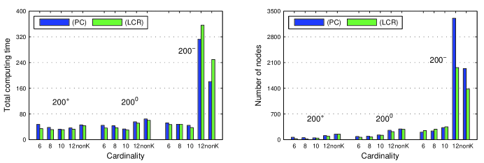
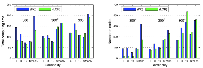
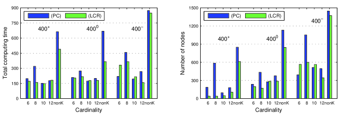
Figure 2: Comparison of total computing time and nodes for (MV).

Figure 2 displays the total computing time and nodes of the two reformulations for (MV). The total computing time for (PC) is the sum of “$({\rm time}_{l})$” and the “time” for (PC), and the total computing time for (LCR) is the sum of “$({\rm time}_{l})$”, “$({\rm time}_{s})$” and the “time” for (LCR).

From Figure 2, we can see that, in terms of the total computing time, (LCR) performs better than (PC) for 25 out of the total 45 cases. If we omit the time for solving the SDP and SOCP and only compare the time of the MIQP solver CPLEX, (LCR) performs better than (PC) for 41 out of the total 45 cases. As the perspective cut approach represents the state-of-the-art, the test result for this (MV) data set confirms that using (LCR) reformulation to solve (P) is also efficient. We need to emphasize that, we have tried our best in our numerical tests to optimize the implementation of the perspective cut approach, as the efficiency of the perspective cut approach depends heavily on its implementation details and also on selected parameters of the MIQP solvers.

For the number of nodes explored in (LCR) and (PC), they closely match each other. We might think that because the relaxations in (LCR) are in general looser than the ones in (PC) at children nodes, the number of nodes explored by (LCR) should be larger than (PC) all the time. However, this might not always be the case because the branching schemes, feasible solution heuristics and the branch-and-bound tree inside CPLEX could be quite different for (PC) and (LCR) and the number of nodes explored could demonstrate a more random pattern.

4.2 Subset selection problem

In this subsection, we compare (PC) and (LCR) for the subset selection problem (SSP) introduced in the introduction section.

We use the $40$ instances of the subset selection problem from zheng2013 with $n=50,100$ and $K=5,10,15,20$, $5$ instances for each $(n,K)$ pair. In those instances, we set $m=2n$. The elements of $A$ are generated from the standard normal distribution $N(0,1)$ and $b=A\beta+\epsilon$ where the elements of $\epsilon$ are generated from the standard normal distribution $N(0,1)$ and the elements of $\beta$ are generated uniformly form $[-1,1]$. The lower and upper bounds for the solution $x_{i},~{}i=1,\ldots,n$, are set, respectively, at $-100$ and $100$, which are sufficiently large for those instances.

Table 2: Numerical results of reformulations for (SSP)

$n$	$K$	$({\rm time}_{l})$	$({\rm time}_{s})$		${\rm(PC)}$			${\rm(LCR)}$
					time	nodes		time	nodes
$50$	5	3.86	0.14		2.90	61		0.35	115
	10	3.58	0.21		9.17	205		1.29	445
	15	3.24	0.20		6.82	119		0.71	218
	20	3.44	0.25		9.20	136		0.77	276
$100$	5	14.39	0.48		8.69	99		3.35	295
	10	14.90	0.37		34.65	334		14.11	993
	15	14.95	0.49		89.46	739		41.38	3767
	20	13.36	0.38		613.27	3737		140.76	11789

Table 2 summarizes the numerical results for the 40 instances of (SSP). Each line reports the average results for $5$ instances for each $(n,K)$ pair. The notations in the table are the same as those in Table 1.

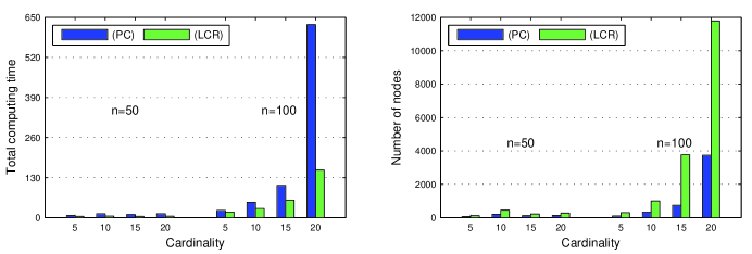
Figure 3: Comparison of total computing time and nodes for (SSP).

Figure 3 displays the total computing time and nodes of the two reformulations for (SSP). The total computing time for (PC) is the sum of “$({\rm time}_{l})$” and the “time” for (PC), and the total computing time for (LCR) is the sum of “$({\rm time}_{l})$”, “$({\rm time}_{s})$” and the “time” for (LCR).

From Figure 3, we can see that although (LCR) explores more nodes than (PC), the total computing time for (LCR) is smaller than that of (PC) in all cases and this advantage of (LCR) over (PC) becomes more apparent as the problem size grows and/or as the cardinality increases. Here for the (SSP) data set, trading off tighter children-node bounds with faster processing time indeed has a good payoff. We also remark again that the efficiency of the perspective cut approach depends heavily on its implementation details and also on the selected parameters of the MIQP solvers. We, however, believe that our new reformulation derived from the lift-and-convexification approach provides a good supplement to the current state-of-the-art approaches.

5 Combination of lift-and-convexification and QCR

In this section, we further combine our lift-and-convexification approach and the QCR approach to derive an even tighter reformulation for (P).

Hammer and Rubin hammer1970 pioneered the QCR approach in the following binary quadratic programs:

$$({\rm BQP})~{}~{}\min ~{}~{}x^{T}Qx+c^{T}x$$

$${\rm s.t.} ~{}~{}Ax=d,$$

$$~{}~{}x_{i}\in\{0,1\},~{}i=1,\ldots,n,$$

where $Q$ is indefinite. In the proposed QCR, they added to the objective function a term $\sum_{i}u(x_{i}^{2}-x_{i})$, where $u$ is a scaler and is chosen to be the negative value of the smallest eigenvalue of $Q$. Billionnet and Elloumi billionnet2007 improved this method by adding the term $\sum_{i}u_{i}(x_{i}^{2}-x_{i})$ with $u_{i}$ being the optimal dual variables of a certain semi-definite program (SDP). Plateauplateau2006reformulations and Billionnet et al.billionnet2008 , billionnet2009qcr also utilized the equality $Ax=d$ in QCR and added the term $\sum_{i}u_{i}(x_{i}^{2}-x_{i})+(Ax-d)^{T}{\rm diag}(w)(Ax-d)$ to the objective, where $u$ and $w$ are chosen to be the dual variables of an enlarged SDP program. Ahlatçıoğlu et al. ahlatcciouglu2012combining proposed to combine QCR and the convex hull relaxation to solve problem (BQP). The geometric investigation in Li et al. li2012 for binary quadratic programs provides some theoretical support for QCR from another angle. Billionnet et al.billionnet2012qcrExtended extended the QCR approach to general mixed-integer programs by using binary decomposition.

To make our discussion more general, we add equality constraints to (P) and consider the following variant of (P):

$$({\rm P^{\prime}})~{}~{}~{}\min ~{}~{}f(x,y):=x^{T}Qx+c^{T}x+h^{T}y$$

$$s.t. ~{}~{}Ax+By\leq d,$$

$$~{}~{}Ex+Fy=g,$$

$$~{}~{}a_{i}y_{i}\leq x_{i}\leq b_{i}y_{i},~{}y_{i}\in\{0,1\},~{}i=1,\ldots,n,$$

where $g\in\Re^{M}$, and $E,F\in\Re^{M\times n}$.

QCR would become beneficial when being applied to the equality and inequality constraints in (P’) on a top of our lift-and-convexification reformulation. Let us consider now the following equivalent reformulation of $({\rm P^{\prime}})$:

$$({\rm P}(u,v,w,t))~{}~{}\min ~{}~{}f(x,y)+\sum_{i=1}^{n}q_{i}(x_{i},y_{i})+(Ex+Fy-g)^{T}{\rm diag}(w)(Ex+Fy-g)$$

$$~{}~{}~{}+(Ax+By+s-d)^{T}{\rm diag}(t)(Ax+By+s-d)$$

$$s.t. ~{}~{}Ax+By+s=d,s\geq 0,$$

$$~{}~{}Ex+Fy=g,$$

$$~{}~{}a_{i}y_{i}\leq x_{i}\leq b_{i}y_{i},~{}y_{i}\in\{0,1\},~{}i=1,\ldots,n,$$

where $q_{i}(x_{i},y_{i})$ is defined in (13).

The best parameter set $(u,v,w,t)$ can be found by solving the following problem:

$$({\rm MAX}uvwt)$$

$$\max\{v({\rm\overline{P}}(u,v,w,t))\mid The~{}objective~{}function~{}of~{}({\rm P}(u,v,w,t))~{}is~{}convex\},$$

where $({\rm\overline{P}}(u,v,w,t))$ is the continuous relaxation of $({\rm P}(u,v,w,t))$.

Using the same technique in the proof for Theorem 3, we can convert the problem $({\rm MAX}uvwt)$ to an SDP problem.

Theorem 7

The problem $({\rm MAX}uvwt)$ is equivalent to the following SDP problem:

$$({\rm SDP}_{a})~{}~{}\max ~{}~{}\tau$$

$${\rm s.t.} ~{}\left(\begin{array}[]{cccc}P_{11}&P_{12}&P_{13}&P_{14}\\ P_{12}^{T}&P_{22}&P_{23}&P_{24}\\ P_{13}^{T}&P_{23}^{T}&P_{33}&P_{34}\\ P_{14}^{T}&P_{24}^{T}&P_{34}^{T}&P_{44}\\ \end{array}\right)\succeq 0,$$ (46)

$$~{}~{}(\delta,\mu,\sigma,\lambda,\pi)\in\Re^{m}_{+}\times\Re^{n}_{+}\times\Re^{n}_{+}\times\Re^{n}_{+}\times\Re^{n}_{+},$$

$$~{}~{}(\eta,\zeta,u,v,\tau)\in\Re^{m}\times\Re^{M}\times\Re^{n}\times\Re^{n}\times\Re,$$

where

$$P_{11} =Q+E^{T}{\rm diag}(w)E+A^{T}{\rm diag}(t)A$$

$$P_{12} =\frac{1}{2}{\rm diag}(u)+E^{T}{\rm diag}(w)F+A^{T}{\rm diag}(t)B$$

$$P_{13} =A^{T}{\rm diag}(t)$$

$$P_{14} =\frac{1}{2}(c-u+A^{T}\eta+E^{T}\zeta-2E^{T}{\rm diag}(w)g+2A^{T}{\rm diag}(t)(-d)-\mu+\sigma)$$

$$P_{22} ={\rm diag}(v)+F^{T}{\rm diag}(w)F+B^{T}{\rm diag}(t)B$$

$$P_{23} =B^{T}{\rm diag}(t)$$

$$P_{24} =\frac{1}{2}(h-v+B^{T}\eta+F^{T}\zeta-2F^{T}{\rm diag}(w)g+2B^{T}{\rm diag}(t)(-d)$$

$$~{}~{}~{}+{\rm diag}(a)\mu-{\rm diag}(b)\sigma-\lambda+\pi)$$

$$P_{33} ={\rm diag}(t)$$

$$P_{34} =\frac{1}{2}(\eta-\delta-2{\rm diag}(t)d)$$

$$P_{44} =-\eta^{T}d-e^{T}\pi-\zeta^{T}g+g^{T}{\rm diag}(w)g+d^{T}{\rm diag}(t)d$$

Proof. We first express $({\rm\overline{P}}(u,v,w,t))$ by its dual form. Associate the following multipliers to the constraints in $({\rm\overline{P}}(u,v,w,t))$:

• $\eta\in\Re^{m}$ for $Ax+By+s=d$;

• $\delta\in\Re^{m}_{+}$ for $s\geq 0$;

• $\zeta\in\Re^{M}$ for $Ex+Fy=g$;

• $\mu_{i}$ and $\sigma_{i}\in\Re_{+}$ for $a_{i}y_{i}\leq x_{i}$ and $x_{i}\leq b_{i}y_{i}$, respectively, $i=1,\ldots,n$;

• $\lambda_{i}$ and $\pi_{i}\in\Re_{+}$ for $y_{i}\geq 0$ and $y_{i}\leq 1$, respectively, $i=1,\ldots,n$.

Let $\mu=(\mu_{1},\ldots,\mu_{n})^{T}$, $\sigma=(\sigma_{1},\ldots,\sigma_{n})^{T}$, $\lambda=(\lambda_{1},\ldots,\lambda_{n})^{T}$ and $\pi=(\pi_{1},\ldots,\pi_{n})^{T}$. Let $\omega$ denote the vector formed by $\delta,\mu,\sigma,\lambda$ and $\pi$. The Lagrangian function of $({\rm\overline{P}}(u,v,w,t))$ is then given by

$$L(x,y,\omega,\eta,\zeta)$$

$$=x^{T}Qx+c^{T}x+h^{T}y+\sum_{i=1}^{n}(u_{i}x_{i}y_{i}+v_{i}y_{i}^{2}-u_{i}x_{i}-v_{i}y_{i})$$

$$~{}~{}~{}+(Ex+Fy-g)^{T}{\rm diag}(w)(Ex+Fy-g)$$

$$~{}~{}~{}+(Ax+By+s-d)^{T}{\rm diag}(t)(Ax+By+s-d)$$

$$~{}~{}~{}+\eta^{T}(Ax+By+s-d)+\delta^{T}(-s)+\zeta^{T}(Ex+Fy-g)$$

$$~{}~{}~{}+\sum_{i=1}^{n}\mu_{i}(a_{i}y_{i}-x_{i})+\sum_{i=1}^{n}\sigma_{i}(x_{i}-b_{i}y_{i})+\sum_{i=1}^{n}\lambda_{i}(-y_{i})+\sum_{i=1}^{n}\pi_{i}(y_{i}-1)$$

$$=(x,y,s)^{T}\left(\begin{array}[]{ccc}P_{11}&P_{12}&A^{T}{\rm diag}(t)\\ P_{12}^{T}&P_{22}&B^{T}{\rm diag}(t)\\ {\rm diag}(t)A&{\rm diag}(t)B&{\rm diag}(t)\\ \end{array}\right)\left(\begin{array}[]{c}x\\ y\\ s\\ \end{array}\right)$$

$$~{}~{}~{}+(c-u+A^{T}\eta+E^{T}\zeta-2E^{T}{\rm diag}(w)g+2A^{T}{\rm diag}(t)(-d)-\mu+\sigma)^{T}x$$

$$~{}~{}~{}+(h-v+B^{T}\eta+F^{T}\zeta-2F^{T}{\rm diag}(w)g+2B^{T}{\rm diag}(t)(-d)$$

$$~{}~{}~{}+{\rm diag}(a)\mu-{\rm diag}(b)\sigma-\lambda+\pi)^{T}y+(\eta-\delta-2{\rm diag}(t)d)^{T}s$$

$$~{}~{}~{}-\eta^{T}d-e^{T}\pi-\zeta^{T}g+g^{T}{\rm diag}(w)g+d^{T}{\rm diag}(t)d.$$

Furthermore, the Lagrangian dual problem of $({\rm\overline{P}}(u,v,w,t))$ can be expressed as

$$\max\{\min_{(x,y,s)\in\Re^{n}\times\Re^{n}\times\Re^{m}}~{}L(x,y,\omega,\eta,\zeta)\mid\omega\geq 0\}.$$ (47)

Introducing an additional variable $\tau$, we can rewrite (47) as

$$\max ~{}~{}\tau$$ (48)

$${\rm s.t.} ~{}~{}\min_{(x,y,s)\in\Re^{n}\times\Re^{n}\times\Re^{m}}~{}L(x,y,\omega,\eta,\zeta)\geq\tau,$$ (49)

$$~{}~{}\omega\geq 0.$$ (50)

We see that the constraint in (49) is equivalent to $L(x,y,\omega,\eta,\zeta)-\tau\geq 0$ for all $x,y$,s, which is further equivalent to

$$L(x/k,y/k,\omega,\eta,\zeta)-\tau\geq 0,~{}~{}\forall(x,y,s)\in\Re^{n}\times\Re^{n}\times\Re^{m},~{}\forall k\in\Re,~{}k\not=0.$$ (51)

Multiplying both sides of (51) by $k^{2}$ yields a homogeneous quadratic form of $(x,y,s,t)$ in the left-hand side of (51). Thus, the constraint in (49) is equivalent to the semidefinite constraint (46). Consequently, the problem in (48)-(50) can be expressed as

$$\max\{\tau\mid{\rm constraint}~{}(\ref{dsA31}),~{}\omega\geq 0\}.$$ (52)

If the objective  function of $({\rm P}(u,v,w,t))$ is convex, by the strong duality of convex quadratic programming (see, e.g., Proposition 6.5.6 in bertsekas2003 ), the optimal values of $({\rm\overline{P}}(u,v,w,t))$ and (52) are equal. Thus, we have shown that problem $({\rm MAX}uvwt)$ is equivalent to an SDP problem in the form of $({\rm SDP}_{a})$. $\Box$

Although this SDP problem $({\rm SDP}_{a})$ is very large and takes time to solve, it only needs to be solved once to get the new reformulation. When the original problem $({\rm P^{\prime}})$ is very difficult to solve, solving this SDP to get a better reformulation can gain overall computational advantage.

To test the effectiveness of the new reformulation, we compare the bounds of $({\rm SDP}_{q})$ and $({\rm SDP}_{a})$ on the portfolio selection problem data set introduced in §4. We use the 30 instances with the least diagonal dominance. For each instance, we impose additional equality constraints by dividing the stocks into 10 sections and demanding only one stock to be invested from each section. Such an additional constraint is a very practical one, as in real life applications portfolios are often constructed by choosing investment opportunities from different industries and sections. We use the following measure for bound improvement,

$${\rm impr.}=\frac{v({\rm SDP}_{a})~{}-~{}v({\rm SDP}_{q})}{{\rm optimal\_objective\_value}~{}-~{}v({\rm SDP}_{q})}.$$

Table 3 shows the bound improvement for the 30 instances, which ranges from $2.5\%$ to $47.1\%$, resulting an average bound improvement around $20\%$. This numerical experiment confirms that combining the lift-and-convexification approach and QCR generates a much tighter reformulation on average.

Table 3: Numerical results of bound improvement from combining lift-and-convexification and QCR

n	inst.	impr.	n	inst.	impr.	n	inst.	impr.
$200^{-}$	1	17.0%	$300^{-}$	1	47.1%	$400^{-}$	1	15.1%
$200^{-}$	2	28.0%	$300^{-}$	2	12.7%	$400^{-}$	2	21.8%
$200^{-}$	3	31.8%	$300^{-}$	3	25.9%	$400^{-}$	3	6.5%
$200^{-}$	4	18.1%	$300^{-}$	4	17.6%	$400^{-}$	4	10.1%
$200^{-}$	5	12.7%	$300^{-}$	5	26.1%	$400^{-}$	5	16.5%
$200^{-}$	6	17.7%	$300^{-}$	6	22.0%	$400^{-}$	6	17.9%
$200^{-}$	7	31.1%	$300^{-}$	7	22.8%	$400^{-}$	7	42.1%
$200^{-}$	8	29.2%	$300^{-}$	8	15.6%	$400^{-}$	8	22.5%
$200^{-}$	9	30.4%	$300^{-}$	9	2.5%	$400^{-}$	9	11.5%
$200^{-}$	10	33.0%	$300^{-}$	10	30.2%	$400^{-}$	10	20.1%
average		24.9%			22.2%			18.4%

6 Concluding remarks

We have developed in this paper the lift-and-
convexification approach to construct a parameterized set of MIQP reformulations for convex quadratic programs with semi-continuous variables. The primary idea behind this approach is to lift the quadratic term in the objective function from the $x$-space to the $(x,y)$-space and to convexify the resulting quadratic function of $(x,y)$. We have proposed an SDP formulation to identify the best MIQP reformulation from among this parameterized set and have proved that the identified best reformulation has a continuous relaxation that is as tight as the continuous relaxation of the well known perspective reformulation. By revealing the relationship between our new reformulation and the perspective reformulation, we further reduce the computational effort required to construct our new reformulation and show that we only need little extra effort to solve an additional SOCP problem when compared to the perspective reformulation. Most importantly, our new reformulation retains the linearly constrained quadratic programming structure of the original mix-integer problem, which facilitates more effective utilization of commercial mixed integer programming solvers and ensures much faster computational time at children nodes in the branch-and-bound searching process. Our preliminary comparison results indicate that the performance of our new reformulation solved in general MIQP solvers is, at least, competitive to the state-of-the-art perspective cut approach in many cases and provides a good supplement to the state-of-the-art approaches. We further combine our lift-and-convexification approach and the quadratic convex reformulation approach in the literature to obtain an even tighter reformulation. In a broader picture, the lift-and-convexification approach offers an efficient solution framework of tight MIQP reformulation which improves the existing literature on the trade-off between the bound quality and computational complexity.

References

- [1] A. Ahlatçıoğlu, M. Bussieck, M. Esen, M. Guignard, J.H. Jagla, and A. Meeraus, Combining QCR and CHR for convex quadratic pure 0–1 programming problems with linear constraints, Annals of operations research, 199 (2012), pp. 33–49.
- [2] M.S. AktüRk, A. Atamtürk, and S. GüRel, A strong conic quadratic reformulation for machine-job assignment with controllable processing times, Operations Research Letters, 37 (2009), pp. 187–191.
- [3] E.J. Anderson and B.S. Cheah, Capacitated lot-sizing with minimum batch sizes and setup times, International Journal of Production Economics, 30 (1993), pp. 137–152.
- [4] T.S. Arthanari and Y. Dodge, Mathematical Programming in Statistics, John Wiley & Sons, New York, 1993.
- [5] D.P. Bertsekas, A. Nedić, and A.E. Ozdaglar, Convex Analysis and Optimization, Athena Scientific Belmont, Mass, 2003.
- [6] D. Bertsimas and R. Shioda, Algorithm for cardinality-constrained quadratic optimization, Computational Optimization and Applications, 43 (2009), pp. 1–22.
- [7] D. Bienstock, Computational study of a family of mixed-integer quadratic programming problems, Mathematical Programming, 74 (1996), pp. 121–140.
- [8] A. Billionnet and S. Elloumi, Using a mixed integer quadratic programming solver for the unconstrained quadratic 0-1 problem, Mathematical Programming, 109 (2007), pp. 55–68.
- [9] A. Billionnet, S. Elloumi, and A. Lambert, Extending the QCR method to general mixed-integer programs, Mathematical programming, 131 (2012), pp. 381–401.
- [10] A. Billionnet, S. Elloumi, and M.C. Plateau, Quadratic 0–1 programming: tightening linear or quadratic convex reformulation by use of relaxations, RAIRO-Operations Research, 42 (2008), pp. 103–121.
- [11] , Improving the performance of standard solvers for quadratic 0-1 programs by a tight convex reformulation: The QCR method, Discrete Applied Mathematics, 157 (2009), pp. 1185–1197.
- [12] B. Blog, G. Van der Hoek, A.H.G. Rinnooy Kan, and G.T. Timmer, The optimal selection of small portfolios, Management Science, 29 (1983), pp. 792–798.
- [13] P. Bonami and M.A. Lejeune, An exact solution approach for portfolio optimization problems under stochastic and integer constraints, Operations Research, 57 (2009), pp. 650–670.
- [14] J. Borwein and A. Lewis, Convex Analysis and Nonlinear Optimization: Theory and Examples, Springer, 2006.
- [15] T.J. Chang, N. Meade, J.E. Beasley, and Y.M. Sharaiha, Heuristics for cardinality constrained portfolio optimisation, Computer & Operations Research, 27 (2000), pp. 1271–1302.
- [16] Y. Crama and M. Schyns, Simulated annealing for complex portfolio selection problems, European Journal of Operational Research, 150 (2003), pp. 546–571.
- [17] X.T. Cui, X.J. Zheng, S.S. Zhu, and X.L. Sun, Convex relaxations and MIQCQP reformulations for a class of cardinality-constrained portfolio selection problems, Journal of Global Optimization, 56 (2013), pp. 1409–1423.
- [18] Inc. CVX Research, CVX: Matlab software for disciplined convex programming, version 2.0. http://cvxr.com/cvx, Aug. 2012.
- [19] A. Fernández and S. Gómez, Portfolio selection using neural networks, Computers & Operations Research, 34 (2007), pp. 1177–1191.
- [20] A. Frangioni, F. Furini, and C. Gentile, Approximated perspective relaxations: A project and lift approach, tech. report, 2013. TR-13-04. Avialable at: http://compass2.di.unipi.it/TR/Files/TR-13-04.pdf.gz.
- [21] A. Frangioni and C. Gentile, Perspective cuts for a class of convex 0–1 mixed integer programs, Mathematical Programming, 106 (2006), pp. 225–236.
- [22] , Solving nonlinear single-unit commitment problems with ramping constraints, Operations Research, 54 (2006), pp. 767–775.
- [23] , SDP diagonalizations and perspective cuts for a class of nonseparable MIQP, Operations Research Letters, 35 (2007), pp. 181–185.
- [24] , A computational comparison of reformulations of the perspective relaxation: SOCP vs. cutting planes, Operations Research Letters, 37 (2009), pp. 206–210.
- [25] A. Frangioni, C. Gentile, E. Grande, and A. Pacifici, Projected perspective reformulations with applications in design problems, Operations Research, 59 (2011), pp. 1225–1232.
- [26] A. Frangioni, C. Gentile, and F. Lacalandra, Solving unit commitment problems with general ramp constraints, International Journal of Electrical Power & Energy Systems, 30 (2008), pp. 316–326.
- [27] , Tighter approximated MILP formulations for unit commitment problems, IEEE Transactions on Power Systems, 24 (2009), pp. 105–113.
- [28] J.J. Gao and D. Li, Cardinality constrained linear-quadratic optimal control, IEEE Transations on Automatical Control, 56 (2011), pp. 1936–1941.
- [29] , Optimal cardinality constrained portfolio selection, Operations Research, 61 (2013), pp. 745–761.
- [30] , A polynomial case of the cardinality-constrained quadratic optimization problem, Journal of Global Optimization, 56 (2013), pp. 1441–1455.
- [31] M. Grant and S. Boyd, Graph implementations for nonsmooth convex programs, in Recent Advances in Learning and Control, V. Blondel, S. Boyd, and H. Kimura, eds., Lecture Notes in Control and Information Sciences, Springer-Verlag Limited, 2008, pp. 95–110. http://stanford.edu/~boyd/graph_dcp.html.
- [32] O. Günlük and J. Linderoth, Perspective reformulations of mixed integer nonlinear programs with indicator variables, Mathematical programming, 124 (2010), pp. 183–205.
- [33] P.L. Hammer and A.A. Rubin, Some remarks on quadratic programming with 0-1 variables, RAIRO-Operations Research-Recherche Opérationnelle, 4 (1970), pp. 67–79.
- [34] N.L. Jacob, A limited-diversification portfolio selection model for the small investor, Journal of Finance, 29 (1974), pp. 847–856.
- [35] N.J. Jobst, M.D. Horniman, C.A. Lucas, and G. Mitra, Computational aspects of alternative portfolio selection models in the presence of discrete asset choice constraints, Quantitative Finance, 1 (2001), pp. 489–501.
- [36] D. Li, X.L. Sun, and C.L. Liu, An exact solution method for unconstrained quadratic 0–1 programming: a geometric approach, Journal of Global Optimization, 52 (2012), pp. 797–829.
- [37] D. Li, X.L. Sun, and J. Wang, Optimal lot solution to cardinality constrained mean-variance formulation for portfolio selection, Mathematical Finance, 16 (2006), pp. 83–101.
- [38] D. Maringer and H. Kellerer, Optimization of cardinality constrained portfolios with a hybrid local search algorithm, OR Spectrum, 25 (2003), pp. 481–495.
- [39] A.J. Miller, Subset Selection in Regression, Chapman and Hall, 2002. Second edition.
- [40] G. Mitra, F. Ellison, and A. Scowcroft, Quadratic programming for portfolio planning: Insights into algorithmic and computational issues. part ii: Processing of portfolio planning models with discrete constraints, Journal of Asset Management, 8 (2007), pp. 249–258.
- [41] Y.W. Park and D. Klabjan, Lot sizing with minimum order quantity, Discrete Applied Mathematics, 181 (2015), pp. 235–254.
- [42] M.C. Plateau, Reformulations quadratiques convexes pour la programmation quadratique en variables 0-1, PhD thesis, Ph. D. thesis, Conservatoire National d Arts et Métiers, 2006.
- [43] A. Schaerf, Local search techniques for constrained portfolio selection problems, Computational Economics, 20 (2002), pp. 177–190.
- [44] D.X. Shaw, S. Liu, and L. Kopman, Lagrangian relaxation procedure for cardinality-constrained portfolio optimization, Optimization Methods and Software, 23 (2008), pp. 411–420.
- [45] X.L. Sun, X.J. Zheng, and D. Li, Recent advances in mathematical programming with semi-continuous variables and cardinality constraint, Journal of the Operations Research Society of China, 1 (2013), pp. 55–77.
- [46] J. Xie, S. He, and S. Zhang, Randomized portfolio selection, with constraints, Pacific Jorunal of Optimization, 4 (2008), pp. 89–112.
- [47] X.J. Zheng, X.L. Sun, and D. Li, Improving the performance of MIQP solvers for quadratic programs with cardinality and minimum threshold constraints: A semidefinite program approach, INFORMS Journal on Computing, 26 (2014), pp. 690–703.