NUMERICAL SOLUTION OF THE TIME-FRACTIONAL FOKKER–PLANCK EQUATION WITH GENERAL FORCING

Abstract

We study two schemes for a time-fractional Fokker–Planck equation with space- and time-dependent forcing in one space dimension. The first scheme is continuous in time and is discretized in space using a piecewise-linear Galerkin finite element method. The second is continuous in space and employs a time-stepping procedure similar to the classical implicit Euler method. We show that the space discretization is second-order accurate in the spatial $L_{2}$-norm, uniformly in time, whereas the corresponding error for the time-stepping scheme is $O(k^{\alpha})$ for a uniform time step $k$, where $\alpha\in(1/2,1)$ is the fractional diffusion parameter. In numerical experiments using a combined, fully-discrete method, we observe convergence behaviour consistent with these results.

1 Introduction

We investigate the numerical solution of the inhomogeneous, time-fractional Fokker–Planck equation [10],

$$u_{t}-\kappa_{\alpha}\partial_{t}^{1-\alpha}u_{xx}+\mu_{\alpha}^{-1}\bigl{(}F\partial_{t}^{1-\alpha}u\bigr{)}_{x}=g,$$ (1)

for $0<x<L$ and $0<t<T$, with initial data $u(x,0)=u_{0}(x)$ and subject to homogeneous Dirichlet boundary conditions $u(0,t)=0=u(L,t)$. (We use subscripts to indicate partial derivatives of integer order with respect to $x$ or $t$; for instance, $u_{t}=\partial u/\partial t$.) The parameter $\kappa_{\alpha}$ is the generalized diffusivity constant, $\mu_{\alpha}$ is the generalized friction constant, and the driving force $F$ and the source term $g$ are permitted to be functions of both $x$ and $t$. The subdiffusion parameter $\alpha$ satisfies $0<\alpha<1$, and the fractional time derivative is interpreted in the Riemann–Liouville sense; thus, $\partial_{t}^{1-\alpha}=(I^{\alpha}v)_{t}$ where $I^{\alpha}$ is the fractional integral of order $\alpha$,

$$I^{\alpha}v(t)=\int_{0}^{t}\omega_{\alpha}(t-s)v(s)\,ds\quad\text{with}\quad\omega_{\alpha}(t)=\frac{t^{\alpha-1}}{\Gamma(\alpha)}.$$

In 1999, Metzler et al. [15] used a discrete master equation to model the behaviour of subdiffusive particles in the presence of a driving force $F(x)$, showing that in the diffusive limit the probability density $u(x,t)$ for a particle to be at position $x$ at time $t$ obeys a fractional Fokker–Planck equation of the form

$$u_{t}-\partial_{t}^{1-\alpha}\bigl{(}\kappa_{\alpha}u_{xx}-\mu_{\alpha}^{-1}\bigl{(}Fu\bigr{)}_{x}\bigr{)}=0.$$ (2)

Subsequently, Henry et al. [10] considered the more general case when $F=F(x,t)$ may depend on $t$ as well as $x$, and showed that $u$ obeys (1) with $g\equiv 0$. The two equations coincide if $F$ is independent of $t$, but if the forcing is time-dependent then (2) does not properly correspond to any physical stochastic process [9].

Various numerical (time stepping finite difference) methods have been proposed for solving (2), usually for $F$ assumed to be either a constant or a function of $x$ only. The starting point was often to rewrite equation (2) in the form

$$I^{1-\alpha}(u_{t})-\kappa_{\alpha}u_{xx}+\mu_{\alpha}^{-1}(Fu)_{x}=0,$$ (3)

in which the first term is a Caputo fractional derivative. Indeed, (3) is in some ways more convenient than (2) for constructing and analyzing the accuracy of numerical schemes. However, the simpler form (3) is not applicable in our case because $F$ may depend on $t$.

For the numerical solution of (3) with $F=F(x)$, Deng [6] transformed the equation to a system of fractional ODEs by discretizing the spatial derivatives and using the properties of Riemann–Liouville and Caputo fractional derivatives, and then applied a predictor-corrector approach combined with the method of lines. This work also presented a stability and convergence analysis. Cao et al. [3] adopted a similar approach for (2) and solved the resulting system of fractional ODEs using a second order, backward Euler scheme. Chen et al. [4] studied the stability and convergence properties of three implicit finite difference techniques, in each of which the diffusion term was approximated by the standard second order difference approximation at the advanced time level. In related work, Jiang [11] established monotonicity properties of the numerical solutions obtained by using these schemes, and so showed that the time-stepping preserves non-negativity of the solution. Based on this property, a new proof of stability and convergence was provided.

Fairweather et al. [8] investigated the stability and convergence of an orthogonal spline collocation method in space combined with the backward Euler method in time, based on the L1 approximation of the fractional derivative. In an earlier work, Saadmandi [17] studied a collocation method based on shifted Legendre polynomials in time and Sinc functions in space. Recently, Vong and Wang [18] have analysed a high order, compact difference scheme for (3), and Cui [5] has considered a more general fractional convection–diffusion equation,

$$I^{1-\alpha}u_{t}-(au_{x})_{x}+bu_{x}+cu=f,$$

with coefficients $a$, $b$, $c$ that may depend on $x$ and $t$, applying a high-order approximation for the time fractional derivative combined with a compact exponential finite difference scheme for approximating the convection and diffusion terms. Stability (using Fourier methods) and an estimate for the local truncation error were obtained in the case of constant coefficients. We are not aware of any previous analysis on the numerical solution of (1) for a general $F$ depending on both $x$ and $t$.

In Section 2 we gather together some preliminary results needed in our subsequent analysis, including continuous and discrete versions of a generalized Gronwall inequality involving the Mittag–Leffler function in place of the usual exponential. One of these results (Lemma 4) holds only for $1/2<\alpha<1$ so much of our theory requires this restriction. Section 3 deals with a spatial discretization of (1) by a continuous, piecewise-linear Galerkin finite element method. We prove stability of the scheme in Theorem 9 and, under weaker assumptions on $F$ but with a worse bound, in Theorem 10. An error estimate follows in Theorem 11 showing second-order accuracy in $L_{\infty}\bigl{(}(0,T),L_{2}(\Omega)\bigr{)}$, where $\Omega=(0,L)$ denotes the spatial interval. We then study a time stepping scheme in Section 4, proving a stability estimate in Theorem 14 and then an error bound in Theorem 15, assuming a constant time step $k$. This scheme, which is continuous in space, is formally first-order accurate but, owing to the weakly singular kernel in the fractional integral, we are able to show only that the error in $L_{2}(\Omega)$ at the $n$th time level is $O(k^{\alpha})$. Section 5 reports on numerical experiments with a fully discrete scheme based on the semi-discrete ones analyzed in Sections 3 and 4. We observe $O(k+h^{2})$ convergence when $\alpha$ is close to $1$, or when we use an appropriately graded mesh in time. The experiments give no evidence that the methods fail if $0<\alpha\leq 1/2$, although the convergence rate deteriorates as $\alpha$ decreases when using a uniform time step. We also apply our method to a problem from a recent paper by Angstmann et al. [1] and investigate whether the regularity of the initial data affects the stability of the methods. A brief appendix proves a technical result (Lemma 17) used in showing stability of the time-stepping procedure.

2 Technical preliminaries

Lemmas 1–4 below summarize some properties of fractional integrals that will be needed in our analysis. In each case, we assume that the function $v(t)$ is defined for $0\leq t\leq T$ and takes values in a Hilbert space with inner product $\langle\cdot,\cdot\rangle$ and norm $\|\cdot\|$, and is sufficiently regular for the integrand on the right-hand side to be absolutely integrable.

Lemma 1.

For $0<\alpha<1$ and $0\leq t\leq T$,

$$\|v(t)-v(0)\|^{2}\leq\frac{t^{1-\alpha}}{1-\alpha}\int_{0}^{t}\|I^{\alpha/2}v_{t}(s)\|^{2}\,ds.$$

Proof.

Put $w(t)=I^{\alpha/2}v_{t}$ so that $v(t)-v(0)=I^{1}v_{t}=I^{1-\alpha/2}w(t)$ and

$$\|v(t)-v(0)\|^{2} \leq\biggl{(}\int_{0}^{t}\omega_{1-\alpha/2}(t-s)\|w(s)\|\,ds\biggr{)}^{2}$$

$$\leq\biggl{(}\int_{0}^{t}\frac{(t-s)^{-\alpha}}{\Gamma(1-\alpha/2)^{2}}\,ds\biggr{)}\biggl{(}\int_{0}^{t}\|w(s)\|^{2}\,ds\biggr{)},$$

giving the desired bound, because $\Gamma(1-\alpha/2)\geq 1$. ∎

Lemma 2.

For $0<\alpha<1$,

$$\int_{0}^{T}\|I^{\alpha/2}v(t)\|^{2}\,dt\leq\frac{1}{\cos(\alpha\pi/2)}\int_{0}^{T}\bigl{\langle}I^{\alpha}v(t),v(t)\bigr{\rangle}\,dt.$$

Proof.

Mustapha and Schötzau [16, Lemma 3.1 (ii)]. ∎

Lemma 3.

For $0<\alpha<1$,

$$\int_{0}^{T}\|I^{\alpha}v(t)\|^{2}\,dt\leq\omega_{\alpha+1}(T)\int_{0}^{T}\omega_{\alpha}(T-t)\int_{0}^{t}\|v(s)\|^{2}\,ds\,dt.$$

Proof.

Since

$$\|I^{\alpha}v(t)\|^{2} \leq\biggl{(}\int_{0}^{t}\omega_{\alpha}(t-s)\|v(s)\|\,ds\biggr{)}^{2}$$

$$\leq\biggl{(}\int_{0}^{t}\omega_{\alpha}(t-s)\,ds\biggr{)}\biggl{(}\int_{0}^{t}\omega_{\alpha}(t-s)\|v(s)\|^{2}\,ds\biggr{)}$$

$$=\omega_{\alpha+1}(t)\int_{0}^{t}\omega_{\alpha}(t-s)\|v(s)\|^{2}\,ds$$

we have

$$\int_{0}^{T}\|I^{\alpha}v(t)\|^{2}\,dt\leq\omega_{\alpha+1}(T)\int_{0}^{T}\int_{0}^{t}\omega_{\alpha}(t-s)\|v(s)\|^{2}\,ds\,dt,$$

and the double integral on the right equals

$$\int_{0}^{T}\|v(s)\|^{2}\int_{s}^{T}\omega_{\alpha}(t-s)\,dt\,ds=\int_{0}^{T}\|v(s)\|^{2}\int_{s}^{T}\omega_{\alpha}(T-t)\,dt\,ds.$$

The result follows after reversing the order of integration again. ∎

Lemma 4.

For $1/2<\alpha<1$,

$$\int_{0}^{T}\|\partial_{t}^{1-\alpha}v(t)\|^{2}\,dt\leq\frac{1}{(2\alpha-1)\Gamma(\alpha)^{2}}\biggl{(}T^{2\alpha-1}\|v(0)\|^{2}+T^{2\alpha}\int_{0}^{T}\|v_{t}\|^{2}\,dt\biggr{)}.$$

Proof.

The identity $\partial_{t}^{1-\alpha}v(t)=v(0)\omega_{\alpha}(t)+I^{\alpha}v_{t}(t)$ implies that

$$\int_{0}^{T}\|\partial_{t}^{1-\alpha}v(t)\|^{2}\,dt\leq 2\|v(0)\|^{2}\int_{0}^{T}\omega_{\alpha}(t)^{2}\,dt+2\int_{0}^{T}\|I^{\alpha}v_{t}\|^{2}\,dt,$$

and the Cauchy–Schwarz inequality gives

$$\int_{0}^{T}\|I^{\alpha}v_{t}\|^{2}\,dt \leq\int_{0}^{T}\biggl{(}\int_{0}^{t}\omega_{\alpha}(t-s)\|v_{t}(s)\|\,ds\biggr{)}^{2}\,dt$$

$$\leq\int_{0}^{T}\biggl{(}\int_{0}^{t}\omega_{\alpha}(t-s)^{2}\,ds\biggr{)}\biggl{(}\int_{0}^{T}\|v_{t}(s)\|^{2}\,ds\biggr{)}\,dt,$$

so it suffices to note that $\int_{0}^{t}\omega_{\alpha}(t-s)^{2}\,ds\leq T^{2\alpha-1}/\bigl{(}(2\alpha-1)\Gamma(\alpha)^{2}\bigr{)}$ for $\alpha>1/2$. ∎

The existence and uniqueness of our spatially discrete solution to (1) will follow from the following result for an $m\times m$ system of weakly singular integral equations. Here, $|\cdot|$ may denote any matrix norm on $\mathbb{R}^{m\times m}$ induced by a norm on $\mathbb{R}^{m}$.

Theorem 5.

There exists a unique continuous solution $\boldsymbol{u}:[0,\infty)\to\mathbb{R}^{m}$ to the linear Volterra integral equation

$$\boldsymbol{u}(t)+\int_{0}^{t}\boldsymbol{K}(t,s)\boldsymbol{u}(s)\,ds=\boldsymbol{g}(t)\quad\text{for $0\leq t<\infty$,}$$

if the following conditions are satisfied:

1. $\boldsymbol{g}:[0,\infty)\to\mathbb{R}^{m}$ is continuous;

2. $\boldsymbol{K}(t,s)\in\mathbb{R}^{m\times m}$ is continuous for $0\leq s<t<\infty$;

3. for any continuous function $\boldsymbol{v}:[0,\infty)\to\mathbb{R}^{m}$, the integrals

   $$\int_{0}^{t}\boldsymbol{K}(t,s)\boldsymbol{v}(s)\,ds\quad\text{and}\quad\int_{0}^{t}|\boldsymbol{K}(t,s)|\,ds$$

   exist and are continuous for $0\leq t<\infty$;

4. there exist constants $\gamma>0$ and $\epsilon>0$ such that

   $$\int_{0}^{t}e^{-\gamma(t-s)}|\boldsymbol{K}(t,s)|\,ds\leq 1-\epsilon\quad\text{for $0\leq t<\infty$.}$$

Proof.

Becker [2, Corollary 2.3]. ∎

Our stability analysis of the spatially discrete solution makes use of the following weakly singular Gronwall inequality, involving the Mittag–Leffler function

$$E_{\beta}(z)=\sum_{n=0}^{\infty}\frac{z^{n}}{\Gamma(1+n\beta)}.$$ (4)

The usual Gronwall inequality is just the special case $\beta=1$, because $E_{1}(z)=e^{z}$.

Lemma 6.

Let $\beta>0$ and $T>0$. Assume that $a$ and $b$ are non-negative and non-decreasing functions on the interval $[0,T]$. If $y:[0,T]\to\mathbb{R}$ is a locally integrable function satisfying

$$0\leq y(t)\leq a(t)+b(t)\int_{0}^{t}\omega_{\beta}(t-s)y(s)\,ds\quad\text{for $0\leq t\leq T$,}$$

then

$$y(t)\leq a(t)E_{\beta}\bigl{(}b(t)t^{\beta}\bigr{)}\quad\text{for $0\leq t\leq T$.}$$

Proof.

Dixon and McKee [7, Theorem 3.1]; Ye, Gao and Ding [19, Corollary 2]. ∎

We also use a discrete version of this Gronwall inequality to establish stability of our time stepping procedure.

Lemma 7.

Let $0<\beta\leq 1$, $N>0$, $k>0$ and $t_{n}=nk$ for $0\leq n\leq N$. Assume that $(A_{n})_{n=0}^{N}$ is a non-negative and non-decreasing sequence, and that $B\geq 0$. If the sequence $(y^{n})_{n=0}^{N}$ satisfies

$$0\leq y^{n}\leq A_{n}+Bk\sum_{j=0}^{n-1}\omega_{\beta}(t_{n}-t_{j})y^{j}\quad\text{for $0\leq n\leq N$,}$$

then

$$y^{n}\leq A_{n}E_{\beta}(Bt_{n}^{\beta})\quad\text{for $0\leq n\leq N$.}$$

Proof.

Dixon and McKee [7, Theorem 6.1]. ∎

3 Spatial discretization

We choose a partition $0=x_{0}<x_{1}<x_{2}<\cdots<x_{P}=L$ of the spatial interval $\Omega=(0,L)$ and denote the length of the $p$th subinterval by $h_{p}=x_{p}-x_{p-1}$ for $1\leq p\leq P$. With $h=\max_{1\leq p\leq P}h_{p}$, we define the usual space $\mathbb{S}_{h}$ of continuous, piecewise-linear functions that satisfy the Dirichlet boundary conditions, so that $\mathbb{S}_{h}\subseteq H^{1}_{0}(\Omega)$. Recall that $F=F(x,t)$ and $g=g(x,t)$. In our notation, we will often suppress the dependence on $x$ and think of $u=u(x,t)$ as a function of $t$ taking values in $L_{2}(\Omega)$. We also assume that $\kappa_{\alpha}=\mu_{\alpha}=1$.

In the usual weak formulation of (1), we seek $u$ satisfying

$$\langle u_{t},v\rangle+\langle\partial_{t}^{1-\alpha}u_{x},v_{x}\rangle-\langle F\partial_{t}^{1-\alpha}u,v_{x}\rangle=\langle g(t),v\rangle\quad\text{for $v\in H^{1}_{0}(\Omega)$,}$$ (5)

with $u(0)=u_{0}$, where $\langle\cdot,\cdot\rangle$ denotes the inner product in $L_{2}(\Omega)$. For our error analysis, it is useful to consider a slightly more general, spatially discrete version of (5), in which $u_{h}:[0,T]\to\mathbb{S}_{h}$ satisfies

$$\langle u_{ht},v\rangle+\langle\partial_{t}^{1-\alpha}u_{hx},v_{x}\rangle-\langle F\partial_{t}^{1-\alpha}u_{h},v_{x}\rangle=\langle g(t),v\rangle+\langle g_{*}(t),v_{x}\rangle\\$$ (6)

for $v\in\mathbb{S}_{h}$, with $u_{h}(0)=u_{0h}$ where $u_{0}\approx u_{0h}\in\mathbb{S}_{h}$, and where $u_{ht}=\partial u_{h}/\partial t$. Thus, if $g_{*}(x,t)\equiv 0$, then $u_{h}$ is the standard Galerkin finite element solution of (5).

To show the existence and uniqueness of $u_{h}$ satisfying (6), define the linear operator $B_{h}(t):\mathbb{S}_{h}\to\mathbb{S}_{h}$ (which depends on $t$ through $F$) by

$$\langle B_{h}(t)v,w\rangle=\langle v_{x},w_{x}\rangle-\langle Fv,w_{x}\rangle\quad\text{for $v$, $w\in\mathbb{S}_{h}$,}$$

and the finite element function $g_{h}(t)\in\mathbb{S}_{h}$ by

$$\langle g_{h}(t),w\rangle=\langle g(t),w\rangle+\langle g_{*}(t),w_{x}\rangle\quad\text{for $w\in\mathbb{S}_{h}$.}$$

The variational equation (6) is then equivalent to

$$u_{ht}+B_{h}(t)\partial_{t}^{1-\alpha}u_{h}=g_{h}(t).$$

Integrating with respect to $t$, we find that $u_{h}$ satisfies the Volterra equation

$$u_{h}(t)+\int_{0}^{t}K_{h}(t,s)u_{h}(s)\,ds=G_{h}(t)\quad\text{for $0\leq t\leq T$,}$$

with the weakly-singular kernel

$$K_{h}(t,s)=B_{h}(t)\omega_{\alpha}(t-s)-\int_{s}^{t}B_{ht}(\tau)\omega_{\alpha}(\tau-s)\,d\tau$$

and right-hand side

$$G_{h}(t)=u_{0h}+\int_{0}^{t}g_{h}(s)\,ds.$$

Theorem 8.

If $F\in W^{1}_{\infty}\bigl{(}(0,T);L_{\infty}(\Omega)\bigr{)}$ and $g$, $g_{*}\in L_{1}\bigl{(}(0,T);L_{2}(\Omega)\bigr{)}$, then for any $u_{0h}\in\mathbb{S}_{h}$ there exists a unique continuous $u_{h}:[0,\infty)\to\mathbb{S}_{h}$ satisfying (6) for all $v\in\mathbb{S}_{h}$, with $u_{h}(0)=u_{0h}$.

Proof.

Let $|\cdot|$ denote any norm on the finite dimensional space $\mathbb{S}_{h}$. Our assumptions on $F$, $g$ and $g_{*}$ ensure that $G_{h}$ satisfies condition 1 of Theorem 5, and that $K_{h}$ satisfies conditions 2 and 3 (after fixing any basis for $\mathbb{S}_{h}$). Furthermore,

$$|K_{h}(t,s)|\leq C_{F,h}\biggl{(}\omega_{\alpha}(t-s)+\int_{s}^{t}\omega_{\alpha}(\tau-s)\,d\tau\biggr{)}=C_{F,h}\bigl{[}\omega_{\alpha}(t-s)+\omega_{1+\alpha}(t-s)\bigr{]},$$

and, denoting the Laplace transform by $\mathcal{L}$,

$$\int_{0}^{t}e^{-\gamma(t-s)}\omega_{\alpha}(t-s)\,ds\leq\int_{0}^{\infty}e^{-\gamma s}\omega_{\alpha}(s)\,ds=\mathcal{L}\omega_{\alpha}(\gamma)=\gamma^{-\alpha},$$

so

$$\int_{0}^{t}e^{-\gamma(t-s)}|K_{h}(t,s)|\,ds\leq C_{F,h}[\gamma^{-\alpha}+\gamma^{-1-\alpha}],$$

and condition 4 follows for $\gamma$ sufficiently large. ∎

Theorem 8 gives no meaningful stability result for $u_{h}(t)$ (because $C_{F,h}$ from the proof grows rapidly as $h\to 0$) but an energy argument yields the following estimate. We use the abbreviation $\|v\|_{r}$ for the norm in $H^{r}(\Omega)$.

Theorem 9.

If, in addition to the assumptions of Theorem 8,

1. $F_{x}(x,t)\geq 0$ for $0<x<L$ and $0<t<T$;

2. $1+F(x,t)^{2}\leq C_{F}$ for $0<x<L$ and $0<t<T$;

3. $1/2<\alpha<1$;

then

$$\|u_{h}(t)-u_{0h}\|^{2}\leq\frac{t^{1-\alpha}}{(1-\alpha)^{2}}\int_{0}^{t}\bigl{(}\tfrac{1}{4}L^{2}\|g(s)\|^{2}+\|g_{*}(s)\|^{2}\bigr{)}\,ds\\ +\frac{C_{F}t^{\alpha}}{(1-\alpha)^{2}(2\alpha-1)}\,\|u_{0h}\|_{1}^{2}\quad\text{for $0<t<T$.}$$

Proof.

Using (6), we find that the function $w_{h}=u_{h}-u_{0h}$ satisfies

$$\bigl{\langle}w_{ht},v\bigr{\rangle}+\langle\partial_{t}^{1-\alpha}w_{hx},v_{x}\rangle-\bigl{\langle}F\partial_{t}^{1-\alpha}w_{h},v_{x}\bigr{\rangle}=\langle g(t),v\rangle+\langle J(t),v_{x}\rangle$$

for all $v\in\mathbb{S}_{h}$, where $J(x,t)=g_{*}(x,t)+F(x,t)\partial_{t}^{1-\alpha}u_{0h}(x)-\partial_{t}^{1-\alpha}(u_{0h})_{x}(x,t)$. Choosing $v=\partial_{t}^{1-\alpha}w_{h}(t)\in\mathbb{S}_{h}$,

$$\bigl{\langle}w_{ht},\partial_{t}^{1-\alpha}w_{h}\bigr{\rangle}+\|\partial_{t}^{1-\alpha}w_{hx}\|^{2}-\bigl{\langle}F\partial_{t}^{1-\alpha}w_{h},\partial_{t}^{1-\alpha}w_{hx}\bigr{\rangle}\\ =\bigl{\langle}g(t),\partial_{t}^{1-\alpha}w_{h}\bigr{\rangle}+\bigl{\langle}J(t),\partial_{t}^{1-\alpha}w_{hx}\bigr{\rangle},$$ (7)

and since $\partial_{t}^{1-\alpha}w_{h}(x,t)=\partial_{t}^{1-\alpha}u_{h}(x,t)-\omega_{\alpha}(t)u_{0h}(x)=0$ if $x\in\{0,L\}$, integration by parts gives

$$\bigl{\langle}F\partial_{t}^{1-\alpha}w_{h},\partial_{t}^{1-\alpha}w_{hx}\bigr{\rangle}=\int_{0}^{L}F\,\tfrac{1}{2}\bigl{(}\bigl{(}\partial_{t}^{1-\alpha}w_{h}\bigr{)}^{2}\bigr{)}_{x}\,dx=-\int_{0}^{L}F_{x}\,\tfrac{1}{2}\bigl{(}\partial_{t}^{1-\alpha}w_{h}\bigr{)}^{2}\,dx.$$

Hence, by assumption 1,

$$\bigl{\langle}w_{ht},\partial_{t}^{1-\alpha}w_{h}\bigr{\rangle}+\|\partial_{t}^{1-\alpha}w_{hx}\|^{2}\leq\bigl{\langle}g(t),\partial_{t}^{1-\alpha}w_{h}\bigr{\rangle}+\bigl{\langle}J(t),\partial_{t}^{1-\alpha}w_{hx}\bigr{\rangle},$$ (8)

and the Poincaré inequality, $\|v\|^{2}\leq\tfrac{1}{2}L^{2}\|v_{x}\|^{2}$ for $v\in H^{1}_{0}(\Omega)$, implies that

$$\bigl{\langle}g(t),\partial_{t}^{1-\alpha}w_{h}\bigr{\rangle}\leq\frac{L^{2}}{4}\|g(t)\|^{2}+\frac{1}{2}\|\partial_{t}^{1-\alpha}w_{hx}\|^{2}.$$

Using $\langle J(t),\partial_{t}^{1-\alpha}w_{hx}\rangle\leq\tfrac{1}{2}\|J(t)\|^{2}+\tfrac{1}{2}\|\partial_{t}^{1-\alpha}w_{hx}\|^{2}$, and noting that $\partial^{1-\alpha}_{t}w_{h}=I^{\alpha}w_{ht}$ because $w_{h}(0)=0$, it follows from (8) that

$$\bigl{\langle}w_{ht},I^{\alpha}w_{ht}\bigr{\rangle}=\bigl{\langle}w_{ht},\partial_{t}^{1-\alpha}w_{h}\bigr{\rangle}\leq\frac{L^{2}}{4}\|g(t)\|^{2}+\frac{1}{2}\|J(t)\|^{2}.$$

By Lemmas 1 and 2, and using the inequality $\cos(\alpha\pi/2)\geq 1-\alpha$,

$$\|w_{h}(T)\|^{2} \leq\frac{T^{1-\alpha}}{(1-\alpha)^{2}}\int_{0}^{T}\bigl{\langle}I^{\alpha}w_{ht},w_{ht}\bigr{\rangle}\,dt$$

$$\leq\frac{T^{1-\alpha}}{(1-\alpha)^{2}}\biggl{(}\frac{L^{2}}{4}\int_{0}^{T}\|g(t)\|^{2}\,dt+\frac{1}{2}\int_{0}^{T}\|J(t)\|^{2}\,dt\biggr{)},$$

and since $(\partial_{t}^{1-\alpha}u_{0h})(x,t)=\omega_{\alpha}(t)u_{0h}(x)$, the Cauchy–Schwarz inequality gives

$$\|J(t)\|\leq\|g_{*}\|+\sqrt{C_{F}}\,\omega_{\alpha}(t)\|u_{0h}\|_{1}.$$

Hence, by assumption 2,

$$\frac{1}{2}\int_{0}^{T}\|J(t)\|^{2}\,dt\leq\int_{0}^{T}\|g_{*}(t)\|^{2}\,dt+C_{F}\|u_{0h}\|^{2}_{1}\int_{0}^{T}\omega_{\alpha}(t)^{2}\,dt,$$ (9)

and assumption 3 means that $\int_{0}^{T}\omega_{\alpha}(t)^{2}\,dt\leq\int_{0}^{T}t^{2\alpha-2}\,dt=T^{2\alpha-1}/(2\alpha-1)$, implying the desired estimate. ∎

For applications, the condition $F_{x}\geq 0$ seems unnaturally restrictive. In the next result, we show that it is not necessary for stability, but the resulting bound grows more rapidly with $t$, owing to the use of the weakly singular Gronwall inequality.

Theorem 10.

If we drop assumption 1 from the hypotheses of Theorem 9, then

$$\|u_{h}(t)-u_{0h}\|^{2}\leq\frac{E_{\alpha/2}\bigl{(}\tfrac{5}{8}C_{F}t^{\alpha}/(1-\alpha)\bigr{)}}{(1-\alpha)^{2}}\biggl{(}t^{1-\alpha}\int_{0}^{t}\bigl{(}\tfrac{1}{2}\|g(s)\|^{2}+\|g_{*}(s)\|^{2}\bigr{)}\,ds\\ +\frac{C_{F}t^{\alpha}}{2\alpha-1}\,\|u_{0h}\|_{1}^{2}\biggr{)}\quad\text{for $0\leq t\leq T$.}$$

Proof.

Recall that $\partial_{t}^{1-\alpha}w_{h}=I^{\alpha}w_{ht}$ because $w_{h}(0)=0$, so (7) implies that

$$\bigl{\langle}I^{\alpha}w_{ht},w_{ht}\bigr{\rangle}\leq\tfrac{1}{2}\|FI^{\alpha}w_{ht}\|^{2}+\tfrac{1}{2}\|g(t)\|^{2}+\tfrac{1}{2}\|I^{\alpha}w_{ht}\|^{2}+\tfrac{1}{2}\|J(t)\|^{2}.$$

By Lemma 2,

$$y_{h}(T)\equiv\smash[b]{\int_{0}^{T}\bigl{\|}I^{\alpha/2}w_{ht}\bigr{\|}^{2}\,dt\leq\frac{1}{1-\alpha}\int_{0}^{T}\bigl{\langle}I^{\alpha}w_{ht},w_{ht}\bigr{\rangle}\,dt},$$

so if we let

$$a(T)=\smash{\frac{1}{2(1-\alpha)}\int_{0}^{T}\bigl{(}\|g(t)\|^{2}+\|J(t)\|^{2}\bigr{)}\,dt}$$

then

$$y_{h}(T)\leq\smash[t]{a(T)+\frac{C_{F}}{2(1-\alpha)}\int_{0}^{T}\|I^{\alpha}w_{ht}\|^{2}\,dt}.$$

Since $I^{\alpha}w_{ht}=I^{\alpha/2}\bigl{(}I^{\alpha/2}w_{ht}\bigr{)}$, Lemma 3 implies that

$$y_{h}(T)\leq a(T)+b(T)\int_{0}^{T}\omega_{\alpha/2}(T-t)y_{h}(t)\,dt\quad\text{where}\quad b(T)=\frac{C_{F}\omega_{\alpha/2+1}(T)}{2(1-\alpha)}.$$

Hence, using Lemma 1 and the Gronwall inequality of Lemma 6,

$$\|w_{h}(t)\|^{2}\leq\frac{t^{1-\alpha}}{1-\alpha}\,y_{h}(t)\leq\frac{t^{1-\alpha}}{1-\alpha}\,a(t)E_{\alpha/2}\bigl{(}b(t)t^{\alpha/2}\bigr{)},$$

and the result follows after using (9) to estimate $a(t)$, because the lower bound $\Gamma(\alpha/2+1)\geq 4/5$ for $1/2<\alpha<1$ implies $b(t)\leq\tfrac{5}{8}C_{F}t^{\alpha/2}/(1-\alpha)$. Note that (9) does not rely on the first assumption $F_{x}\geq 0$ of Theorem 9. ∎

To estimate the error in the finite element solution, we will compare $u_{h}(t)$ to the Ritz projection of $u(t)$. Recall that $R_{h}:H^{1}_{0}(\Omega)\to\mathbb{S}_{h}$ is defined by

$$\bigl{\langle}(R_{h}w)_{x},v_{x}\bigr{\rangle}=\langle w_{x},v_{x}\rangle\quad\text{for all $v\in\mathbb{S}_{h}$,}$$

and satisfies

$$\|v-R_{h}v\|\leq Ch^{r}|v|_{r}\quad\text{and}\quad\|(v-R_{h}v)_{x}\|\leq Ch^{r-1}|v|_{r}$$ (10)

for $r\in\{1,2\}$ (in our piecewise-linear case). Here, $|v|_{r}=\|v^{(r)}\|$ is the usual $H^{r}$-seminorm. The next theorem shows that if we choose $u_{0h}=R_{h}u_{0}$, and if $u\in H^{1}\bigl{(}(0,T),H^{r}(\Omega)\bigr{)}$, then $\|u_{h}(t)-u(t)\|=O(h^{r})$ for $0\leq t\leq T$ and $r\in\{1,2\}$.

Theorem 11.

Let $u_{h}$ denote the the spatially-discrete finite element solution of (1), defined by (6) with $g_{*}(t)\equiv 0$. Then, under the hypotheses of Theorem 10, we have the error bound

$$\|u_{h}(t)-u(t)\|^{2}\leq C\|u_{0h}-R_{h}u_{0}\|_{1}^{2}+Ch^{2r}\biggl{(}\|u_{0}\|_{r}^{2}+\int_{0}^{t}\|u_{t}(s)\|_{r}^{2}\,ds\biggr{)}$$

for $0\leq t\leq T$ and $r\in\{1,2\}$, where $C$ depends on $\alpha$, $F$, $T$ and $L$.

Proof.

We decompose the error into two terms,

$$u_{h}-u=\theta+\rho\quad\text{where}\quad\theta=u_{h}-R_{h}u\quad\text{and}\quad\rho=R_{h}u-u,$$

and deduce from (6) that, for $v\in\mathbb{S}_{h}$,

$$\langle\theta_{t},v\rangle+\bigl{\langle}\partial_{t}^{1-\alpha}\theta_{x},v_{x}\bigr{\rangle}-\bigl{\langle}F\partial_{t}^{1-\alpha}\theta,v_{x}\bigr{\rangle}=\langle g(t),v\rangle\\ -\langle R_{h}u_{t},v\rangle-\bigl{\langle}\partial_{t}^{1-\alpha}(R_{h}u)_{x},v_{x}\bigr{\rangle}+\bigl{\langle}F\partial_{t}^{1-\alpha}R_{h}u,v_{x}\bigr{\rangle}.$$

Since $\bigl{\langle}\partial_{t}^{1-\alpha}(R_{h}u)_{x},v_{x}\bigr{\rangle}=\bigl{\langle}(R_{h}\partial_{t}^{1-\alpha}u)_{x},v_{x}\bigr{\rangle}=\bigl{\langle}\partial_{t}^{1-\alpha}u_{x},v_{x}\bigr{\rangle}$, it follows from (5) that $\theta:[0,T]\to\mathbb{S}_{h}$ satisfies

$$\langle\theta_{t},v\rangle+\bigl{\langle}\partial_{t}^{1-\alpha}\theta_{x},v_{x}\bigr{\rangle}-\bigl{\langle}F\partial_{t}^{1-\alpha}\theta,v_{x}\bigr{\rangle}=\bigl{\langle}F\partial_{t}^{1-\alpha}\rho,v_{x}\bigr{\rangle}-\langle\rho_{t},v\rangle,$$

which has the same form as (6), with $\theta$, $-\rho_{t}$ and $F\partial_{t}^{1-\alpha}\rho$ playing the roles of $u_{h}$, $g(t)$ and $g_{*}(t)$, respectively. Hence, Theorem 10 gives

$$\|\theta(T)-\theta(0)\|^{2}\leq C\|\theta(0)\|_{1}^{2}+C\int_{0}^{T}\bigl{(}\|\rho_{t}\|^{2}+\|\partial_{t}^{1-\alpha}\rho\|^{2}\bigr{)}\,dt,$$

and by Lemma 4, $\int_{0}^{T}\|\partial_{t}^{1-\alpha}\rho\|^{2}\,dt\leq C\|\rho(0)\|^{2}+C\int_{0}^{T}\|\rho_{t}\|^{2}\,dt$. The desired error bound follows after applying (10) with $v=u_{t}$. ∎

4 An implicit time-stepping scheme

To discretize in time, we suppose $0=t_{0}<t_{1}<t_{2}<\cdots<t_{N}=T$ and denote by $k_{n}=t_{n}-t_{n-1}$ the length of the $n$th subinterval $I_{n}=(t_{n-1},t_{n})$, for $1\leq n\leq N$. The maximum time step is denoted by $k=\max_{1\leq n\leq N}k_{n}$. With any sequence of values $v^{1}$, $v^{2}$, …, $v^{N}$ we associate the piecewise-constant functions $\check{v}$ and $\hat{v}$ defined by

$$\check{v}(t)=v^{n}\quad\text{and}\quad\hat{v}(t)=v^{n-1}\quad\text{for $t_{n-1}<t<t_{n}$.}$$ (11)

Integrating the fractional Fokker–Planck equation (1) over the $n$th time interval $I_{n}$ gives

$$u(t_{n})-u(t_{n-1})-\int_{I_{n}}\partial_{t}^{1-\alpha}u_{xx}\,dt+\int_{I_{n}}\bigl{(}F\partial_{t}^{1-\alpha}u\bigr{)}_{x}\,dt=\int_{I_{n}}g(t)\,dt.$$ (12)

We seek to compute $U^{n}(x)\approx u(x,t_{n})$ for $n=1$, $2$, …, $N$ by requiring that

$$U^{n}-U^{n-1}-\int_{I_{n}}\partial_{t}^{1-\alpha}\check{U}_{xx}\,dt+\int_{I_{n}}\bigl{(}F^{n}\partial_{t}^{1-\alpha}\check{U}\bigr{)}_{x}\,dt=k_{n}\bar{g}^{n},$$ (13)

with $F^{n}(x)=F(x,t_{n})$ and $\bar{g}^{n}\approx k_{n}^{-1}\int_{I_{n}}g(t)\,dt$. The time stepping starts from the initial condition

$$U^{0}(x)=u_{0}(x)\quad\text{for $0\leq x\leq L$,}$$ (14)

and is subject to the boundary conditions $U^{n}(0)=0=U^{n}(L)$ for $1\leq n\leq N$.

Since

$$I^{\alpha}\check{v}(t_{n})=\sum_{j=1}^{n}\int_{I_{j}}\omega_{\alpha}(t_{n}-s)v^{j}\,ds=\sum_{j=1}^{n}\omega_{nj}v^{j}$$

where

$$\omega_{nj}=\int_{I_{j}}\omega_{\alpha}(t_{n}-s)\,ds=\omega_{1+\alpha}(t_{n}-t_{j-1})-\omega_{1+\alpha}(t_{n}-t_{j})\quad\text{for $n\geq 2$,}$$

with $\omega_{11}=\omega_{1+\alpha}(t_{1})$, we see that

$$\int_{I_{n}}\partial_{t}^{1-\alpha}\check{v}\,dt=(I^{\alpha}\check{v})(t_{n})-(I^{\alpha}\check{v})(t_{n-1})=\sum_{j=1}^{n}\omega_{nj}v^{j}-\sum_{j=1}^{n-1}\omega_{n-1,j}v^{j}.$$

Hence, to find $U^{n}$ satisfying (13) we solve

$$U^{n}-\omega_{nn}U^{n}_{xx}+\omega_{nn}(F^{n}U^{n})_{x}=U^{n-1}+k_{n}\bar{g}^{n}+\sum_{j=1}^{n-1}(\omega_{nj}-\omega_{n-1,j})\bigl{(}U^{j}_{xx}-(F^{n}U^{j})_{x}\bigr{)}.$$

It follows from Theorem 14 below that this linear elliptic boundary-value problem has a unique solution $U^{n}\in H^{1}_{0}(\Omega)$ if $k$ is sufficiently small. Note that if the mesh is uniform, that is, if $k=k_{n}$ for all $n$, then the sums are discrete convolutions because

$$\omega_{nj}=\frac{k^{\alpha}a_{n-j}}{\Gamma(1+\alpha)}=\omega_{\alpha+1}(k)a_{n-j}\quad\text{where}\quad a_{n}=(n+1)^{\alpha}-n^{\alpha}.$$ (15)

The next two lemmas, which will help prove a stability estimate for $U^{n}$, use the following notation for the backward difference,

$$\partial v(t)=\partial v^{n}=\frac{v^{n}-v^{n-1}}{k_{n}}\quad\text{for $t\in I_{n}$.}$$

Lemma 12.

For any sequence $(v^{n})_{n=0}^{N}$ in $L_{2}(\Omega)$,

$$\sum_{n=1}^{N}k_{n}\|(I^{\alpha}\partial v)(t_{n})\|^{2}\leq 2\omega_{\alpha+1}(T)\sum_{n=1}^{N}\omega_{Nn}\sum_{j=1}^{n}k_{j}\|\partial v^{j}\|^{2}+2\sum_{n=1}^{N}k_{n}^{2\alpha+1}\|\partial v^{n}\|^{2}.$$

Proof.

For $t\in I_{n}$,

$$\|(I^{\alpha}\partial v)(t_{n})\| \leq\int_{0}^{t}\omega_{\alpha}(t-s)\|\partial v(s)\|\,ds+\int_{t}^{t_{n}}\omega_{\alpha}(t_{n}-s)\|\partial v(s)\|\,ds$$

$$=(I^{\alpha}\|\partial v\|)(t)+\omega_{\alpha+1}(t_{n}-t)\|\partial v^{n}\|,$$

where we used the fact that $\omega_{\alpha}(t_{n}-s)\leq\omega_{\alpha}(t-s)$ because $t\leq t_{n}$. Thus, after squaring and integrating over $t\in I_{n}$, we obtain

$$k_{n}\|(I^{\alpha}\partial v)(t_{n})\|^{2}=\int_{I_{n}}\|(I^{\alpha}\partial v)(t_{n})\|^{2}\,dt\leq 2\int_{I_{n}}(I^{\alpha}\|\partial v\|)^{2}\,dt+2k_{n}^{2\alpha+1}\|\partial v^{n}\|^{2},$$

since $(2\alpha+1)\Gamma(\alpha+1)^{2}\geq 1$. By Lemma 3,

$$\sum_{n=1}^{N}k_{n}\|(I^{\alpha}\partial v)(t_{n})\|^{2}\leq 2\omega_{\alpha+1}(T)\int_{0}^{T}\omega_{\alpha}(T-t)\int_{0}^{t}\|\partial v(s)\|^{2}\,ds\,dt\\ +2\sum_{n=1}^{N}k_{n}^{2\alpha+1}\|\partial v^{n}\|^{2},$$

and the result follows because $\int_{I_{j}}\|\partial v(s)\|^{2}\,ds=k_{j}\|\partial v^{j}\|^{2}$. ∎

Lemma 13.

For uniform time steps $k_{n}=k$ and for any sequence $(v_{n})_{n=0}^{N}$,

$$\int_{I_{n}}\partial_{t}^{1-\alpha}\check{v}\,dt=k(I^{\alpha}\partial v)(t_{n})+\omega_{n1}v^{0}$$

and

$$\sum_{n=1}^{N}\langle v^{n},(I^{\alpha}\check{v})(t_{n})\rangle\geq\tfrac{1}{2}\omega_{1+\alpha}(k)\sum_{n=1}^{N}\|v^{n}\|^{2}.$$

Proof.

It follows from (15) that $\omega_{n-1,j-1}=\omega_{nj}$. Thus,

$$I^{\alpha}\check{v}(t_{n-1})=\sum_{j=1}^{n-1}\omega_{n-1,j}v^{j}=\sum_{j=2}^{n}\omega_{n-1,j-1}v^{j-1}=\sum_{j=2}^{n}\omega_{n,j}v^{j-1}=I^{\alpha}\hat{v}(t_{n})-\omega_{n1}v^{0}$$

and so

$$\int_{I_{n}}\partial_{t}^{1-\alpha}\check{v}\,dt=I^{\alpha}\check{v}(t_{n})-I^{\alpha}\check{v}(t_{n-1})=I^{\alpha}(\check{v}-\hat{v})(t_{n})+\omega_{n1}v^{0},$$

which gives the first result because $\check{v}-\hat{v}=k\partial v$. To prove the second result, use (15) to write $(I^{\alpha}\check{v})(t_{n})=\omega_{\alpha+1}(k)\sum_{j=1}^{n}a_{n-j}v^{j}$ and apply Lemma 17 (from Appendix A) to deduce that, pointwise in $x$,

$$\sum_{n=1}^{N}v^{n}I^{\alpha}\check{v}(t_{n})=\omega_{\alpha+1}(k)\sum_{n=1}^{N}\sum_{j=1}^{n}a_{n-j}v^{n}v^{j}\geq\tfrac{1}{2}\omega_{\alpha+1}(k)\sum_{n=1}^{N}(v^{n})^{2}.$$

The desired inequality follows after integrating over $\Omega$. ∎

We are now able to show the following stability estimate.

Theorem 14.

Assume $1/2<\alpha\leq 1$ and consider the implicit scheme (13) in the case of uniform time steps $k_{n}=k$. If $U^{0}\in H^{1}_{0}(\Omega)\cap H^{2}(\Omega)$ and

$$1+F(x,t_{n})^{2}+F_{x}(x,t_{n})^{2}\leq C_{F}\quad\text{for $0<x<L$ and $1\leq n\leq N$,}$$

and if $k$ is sufficiently small, then for $1\leq n\leq N$,

$$\|U^{n}-U^{0}\|^{2}\leq t_{n}E_{\alpha}\biggl{(}\frac{C_{1}t_{n}^{2\alpha}}{\Gamma(\alpha+1)}\biggr{)}\biggl{[}C_{2}\sum_{j=1}^{n}k\|\bar{g}^{j}\|^{2}+C_{3}\|U^{0}\|_{2}^{2}\biggl{(}1+\frac{t_{n}^{2\alpha-1}}{2\alpha-1}\biggr{)}\biggr{]},$$

where $C_{1}=24C_{F}(1+2C_{F})$, $C_{2}=6(1+2C_{F})$ and $C_{3}=6C_{F}(1+4C_{F})$.

Proof.

Put $W^{n}=U^{n}-U^{0}$. Since the mesh is uniform and $W^{0}=0$, Lemma 13 implies that

$$\int_{I_{n}}\partial_{t}^{1-\alpha}\check{U}_{xx}\,dt=\int_{I_{n}}\partial_{t}^{1-\alpha}\check{W}_{xx}\,dt+U^{0}_{xx}\int_{I_{n}}\omega_{\alpha}(t)\,dt=k(I^{\alpha}\partial W_{xx})(t_{n})+\omega_{n1}U^{0}_{xx},$$

and similarly

$$\int_{I_{n}}\bigl{(}F^{n}\partial_{t}^{1-\alpha}\check{U}\bigr{)}_{x}\,dt=k\bigl{(}F^{n}I^{\alpha}(\partial U)(t_{n})\bigr{)}_{x}+\omega_{n1}(F^{n}U^{0})_{x}.$$

Thus, putting $\Phi^{n}=U^{0}_{x}-F^{n}U^{0}$, our time-stepping scheme (13) implies that

$$k\,\partial W^{n}-k(I^{\alpha}\partial W_{xx})(t_{n}) =U^{n}-U^{n-1}-\int_{I_{n}}\partial_{t}^{1-\alpha}\check{U}_{xx}\,dt+\omega_{n1}U^{0}_{xx}$$ (16)

$$=k\bar{g}^{n}-\int_{I_{n}}\bigl{(}F^{n}I^{\alpha}\check{U}\bigr{)}_{x}\,dt+\omega_{n1}U^{0}_{xx}$$

$$=k\bar{g}^{n}-k\bigl{(}F^{n}(I^{\alpha}\partial W)(t_{n})\bigr{)}_{x}+\omega_{n1}\Phi_{x}^{n}.$$

We take the inner product of both sides of (16) with $(I^{\alpha}\partial W)(t_{n})$, then integrate by parts with respect to $x$ and use the fact that $W^{n}(0)=0=W^{n}(L)$ to arrive at

$$k\bigl{\langle}\partial W^{n} ,(I^{\alpha}\partial W)(t_{n})\bigr{\rangle}+k\|(I^{\alpha}\partial W_{x})(t_{n})\|^{2}$$

$$=k\langle\bar{g}^{n},(I^{\alpha}\partial W)(t_{n})\rangle+\bigl{\langle}kF^{n}(I^{\alpha}\partial W)(t_{n})-\omega_{n1}\Phi^{n},(I^{\alpha}\partial W_{x})(t_{n})\bigr{\rangle}$$

$$\leq\tfrac{1}{2}k\|\bar{g}^{n}\|^{2}+\tfrac{1}{2}k\|(I^{\alpha}\partial W)(t_{n})\|^{2}$$

$$\qquad{}+\tfrac{1}{2}k^{-1}\bigl{(}k\|F^{n}(I^{\alpha}\partial W)(t_{n})\|+\omega_{n1}\|\Phi^{n}\|\bigr{)}^{2}+\tfrac{1}{2}k\|(I^{\alpha}\partial W_{x})(t_{n})\|^{2}.$$

Since $\|\Phi^{n}\|^{2}\leq(1+\|F^{n}\|^{2}_{L_{\infty}(\Omega)})\|U^{0}\|_{1}^{2}$,

$$k\bigl{\langle}\partial W^{n},(I^{\alpha}\partial W)(t_{n})\bigr{\rangle}+\tfrac{1}{2}k\|(I^{\alpha}\partial W_{x})(t_{n})\|^{2}\leq\tfrac{1}{2}k\|\bar{g}^{n}\|^{2}\\ +\bigl{(}1+\|F^{n}\|_{L_{\infty}(\Omega)}^{2}\bigr{)}\bigl{(}k\|(I^{\alpha}\partial W)(t_{n})\|^{2}+k^{-1}\omega_{n1}^{2}\|U^{0}\|_{1}^{2}\bigr{)},$$

so after summing over $n$ and applying the second part of Lemma 13, we see that

$$\sum_{n=1}^{N}k\|(I^{\alpha}\partial W_{x})(t_{n})\|^{2}\leq\sum_{n=1}^{N}k\|\bar{g}^{n}\|^{2}+2C_{F}\sum_{n=1}^{N}k\|(I^{\alpha}\partial W)(t_{n})\|^{2}\\ +2C_{F}\|U^{0}\|_{1}^{2}\sum_{n=1}^{N}k^{-1}\omega_{n1}^{2}.$$ (17)

Recall from (15) that $\omega_{n1}=\omega_{\alpha+1}(k)a_{n-1}$ with $a_{n}=(n+1)^{\alpha}-n^{\alpha}$, and observe that $a_{n}\leq\alpha n^{\alpha-1}$ for $n\geq 1$. Thus, for $k$ sufficiently small,

$$\sum_{n=1}^{N}k^{-1}\omega_{n1}^{2} =\frac{k^{2\alpha-1}}{\Gamma(\alpha+1)^{2}}\sum_{n=0}^{N-1}a_{n}^{2}\leq\frac{k^{2\alpha-1}}{\Gamma(\alpha+1)^{2}}\biggl{(}1+(2^{\alpha}-1)^{2}+\sum_{n=2}^{N-1}(\alpha n^{\alpha-1})^{2}\biggr{)}$$ (18)

$$\leq 1+\frac{k^{2\alpha-1}}{\Gamma(\alpha)^{2}}\int_{1}^{N-1}y^{2\alpha-2}\,dy\leq 1+\frac{t_{N-1}^{2\alpha-1}}{2\alpha-1},$$

where, in the final step, we used the assumption that $1/2<\alpha<1$ and the fact that $\Gamma(\alpha)\geq 1$.

In a similar fashion, we next take the inner product of (16) with $\partial W^{n}$ to obtain

$$k\|\partial W^{n}\|^{2} +k\bigl{\langle}(I^{\alpha}\partial W_{x})(t_{n}),\partial W_{x}^{n}\bigr{\rangle}$$

$$=k\langle\bar{g}^{n},\partial W^{n}\rangle-\bigl{\langle}k\bigl{(}F^{n}(I^{\alpha}\partial W)(t_{n})\bigr{)}_{x},\partial W^{n}\bigr{\rangle}+\langle\omega_{n1}\Phi_{x}^{n},\partial W^{n}\rangle$$

$$\leq\tfrac{3}{2}k\|\bar{g}^{n}\|^{2}+\tfrac{3}{2}k\bigl{\|}F^{n}_{x}(I^{\alpha}\partial W)(t_{n})+F^{n}(I^{\alpha}\partial W_{x})(t_{n})\bigr{\|}^{2}$$

$$\qquad{}+\tfrac{3}{2}k^{-1}\omega_{n1}^{2}\|\Phi^{n}_{x}\|^{2}+(\tfrac{1}{6}+\tfrac{1}{6}+\tfrac{1}{6})k\|\partial W^{n}\|^{2}$$

and hence

$$\tfrac{1}{2}k\|\partial W^{n}\|^{2}+k\bigl{\langle}(I^{\alpha}\partial W_{x})(t_{n}),\partial W^{n}_{x}\bigr{\rangle}\leq\tfrac{3}{2}k\|\bar{g}^{n}\|^{2}+\tfrac{3}{2}k^{-1}\omega_{n1}^{2}\|\Phi^{n}_{x}\|^{2}\\ +3k\|F^{n}_{x}\|_{L_{\infty}(\Omega)}^{2}\|(I^{\alpha}\partial W)(t_{n})\|^{2}+3k\|F^{n}\|_{\infty}^{2}\|(I^{\alpha}\partial W_{x})(t_{n})\|^{2}.$$

Since $\|\Phi^{n}_{x}\|^{2}=\|U^{0}_{xx}-F^{n}_{x}U^{0}-F^{n}U^{0}_{x}\|^{2}\leq C_{F}\|U^{0}\|_{2}^{2}$, after summing over $n$ it follows from the second part of Lemma 13 that

$$Y^{N}\equiv\sum_{n=1}^{N}k\|\partial W^{n}\|^{2}\leq 3\sum_{n=1}^{N}k\|\bar{g}^{n}\|^{2}+3C_{F}\|U^{0}\|_{2}^{2}\sum_{n=1}^{N}k^{-1}\omega_{n1}^{2}\\ +6C_{F}\sum_{n=1}^{N}k\|(I^{\alpha}\partial W)(t_{n})\|^{2}+6C_{F}\sum_{n=1}^{N}k\|(I^{\alpha}\partial W_{x})(t_{n})\|^{2},$$

which, together with (17) and (18), implies that

$$Y^{N}\leq\tfrac{1}{2}A_{N}+\tfrac{1}{4}C_{1}\sum_{n=1}^{N}k\|(I^{\alpha}\partial W)(t_{n})\|^{2},$$

where

$$A_{N}=C_{2}\sum_{n=1}^{N}k\|\bar{g}^{n}\|^{2}+C_{3}\|U^{0}\|^{2}_{2}\biggl{(}1+\frac{t_{N}^{2\alpha-1}}{2\alpha-1}\biggr{)}.$$

Hence, by Lemma 12,

$$Y^{N} \leq\tfrac{1}{2}A_{N}+\tfrac{1}{2}C_{1}\biggl{(}\omega_{\alpha+1}(T)\sum_{n=1}^{N}\omega_{Nn}Y^{n}+\sum_{n=1}^{N}k^{2\alpha+1}\|\partial W^{n}\|^{2}\biggr{)}$$

$$\leq\tfrac{1}{2}A_{N}+\tfrac{1}{2}C_{1}\omega_{\alpha+1}(T)\sum_{n=1}^{N-1}\omega_{Nn}Y^{n}+\tfrac{1}{2}C_{1}\bigl{(}\omega_{\alpha+1}(T)\omega_{NN}+k^{2\alpha}\bigr{)}Y^{N}.$$

For $k$ sufficiently small, the term in $Y^{N}$ on the right-hand side is bounded by $\tfrac{1}{2}Y^{N}$. Therefore, because $\omega_{Nn}\leq k^{\alpha}(N-n)^{\alpha-1}/\Gamma(\alpha)$,

$$Y^{N}\leq A_{N}+\frac{B_{N}k^{\alpha}}{\Gamma(\alpha)}\sum_{n=1}^{N-1}(N-n)^{\alpha-1}Y^{n}\quad\text{where}\quad B_{N}=C_{1}\omega_{\alpha+1}(t_{N}),$$

and so

$$Y^{n}\leq A_{n}+B_{N}k\sum_{j=0}^{n-1}\omega_{\alpha}(t_{n}-t_{j})Y^{j}\quad\text{for $0\leq n\leq N$.}$$

Thus, by Lemma 7, $Y^{N}\leq A_{N}E_{\alpha}\bigl{(}B_{N}t_{N}^{\alpha}\bigr{)}=A_{N}E_{\alpha}\bigl{(}C_{1}t_{N}^{2\alpha}/\Gamma(\alpha+1)\bigr{)}$. Finally,

$$\|W^{n}\|^{2}=\biggl{\|}\sum_{j=1}^{n}k\partial W^{j}\biggr{\|}^{2}\leq\biggl{(}\sum_{j=1}^{n}k\biggr{)}\biggl{(}\sum_{j=1}^{n}k\|\partial W^{j}\|^{2}\biggr{)}=t_{n}Y^{n},$$

and the result follows. ∎

We can now prove the following error bound, which implies

$$\|U^{n}-u(t_{n})\|=O(k^{\alpha}),$$

if $u$ is sufficiently regular and if $\|\bar{g}^{j}-g(t)\|\leq Ck^{\alpha}$ for $t\in I_{j}$; recall that $|v|_{r}=\|v^{(r)}\|$.

Theorem 15.

Assume $1/2<\alpha\leq 1$ and consider the implicit scheme (13) in the case of uniform time steps $k_{n}=k$. If $F\in L_{\infty}\bigl{(}(0,T),W^{1}_{\infty}(\Omega)\bigr{)}$, and if $k$ is sufficiently small, then for $0\leq t_{n}\leq T$,

$$\|U^{n}-u(t_{n})\|^{2}\leq C\sum_{j=1}^{n}\int_{I_{j}}\|\bar{g}^{j}-g(t)\|^{2}\,dt+Ck^{2\alpha-1}\int_{0}^{k}t|u_{t}|_{2}^{2}\,dt\\ +Ck^{2\alpha}\int_{k}^{t_{n}}|u_{t}|_{2}^{2}\,dt+Ck^{2}\|u_{0}\|_{1}^{2}+Ck^{2\alpha}\int_{0}^{t_{n}}\|u_{t}\|_{1}^{2}\,dt,$$

where $C$ depends on $\alpha$, $F$ and $T$.

Proof.

Denote the error at the $n$th time level by $e^{n}=U^{n}-u(t_{n})$. Subtracting (12) from (13) yields

$$e^{n}-e^{n-1}-\int_{I_{n}}\partial_{t}^{1-\alpha}\check{e}_{xx}\,dt+\int_{I_{n}}\bigl{(}F^{n}\partial_{t}^{1-\alpha}\check{e}\bigr{)}_{x}\,dt=k\rho^{n},$$

where $\rho^{n}=\rho^{n}_{1}+\rho^{n}_{2}+\rho^{n}_{3}$ for

$$\rho_{1}^{n}=\bar{g}^{n}-\frac{1}{k}\int_{I_{n}}g(t)\,dt,\qquad\rho_{2}^{n}=\frac{1}{k}\int_{I_{n}}\partial_{t}^{1-\alpha}(\check{u}-u)_{xx}\,dt,$$

$$\rho_{3}^{n}=\frac{1}{k}\int_{I_{n}}\bigl{(}F\partial_{t}^{1-\alpha}u-F^{n}\partial_{t}^{1-\alpha}\check{u}\bigr{)}_{x}\,dt.$$

Applying Theorem 14, with $e^{n}$ and $\rho^{n}$ playing the roles of $U^{n}$ and $\bar{g}^{n}$, and noting that $e^{0}=0$ by (14), we see that

$$\|e^{N}\|^{2}\leq C\sum_{n=1}^{N}k\|\rho^{n}\|^{2}\quad\text{for $1\leq n\leq N$.}$$ (19)

Since $\rho^{n}_{1}=k^{-1}\int_{I_{n}}(\bar{g}^{n}-g)\,dt$, we have

$$\sum_{n=1}^{N}k\|\rho^{n}_{1}\|^{2}\leq\sum_{n=1}^{N}\int_{I_{n}}\|\bar{g}^{n}-g\|^{2}\,dt,$$ (20)

and if we put

$$\Lambda_{n}(s)=\begin{cases}\omega_{\alpha}(t_{n}-s),&t_{n-1}<s<t_{n},\\ \omega_{\alpha}(t_{n}-s)-\omega_{\alpha}(t_{n-1}-s),&0<s<t_{n-1},\end{cases}$$

and $\delta_{nj}(t)=(t-t_{j-1})^{-1/2}\int_{t_{j-1}}^{t}\Lambda_{n}(s)\,ds$ for $t\in I_{j}$, then

$$k\rho^{n}_{2} =I^{\alpha}(\check{u}-u)_{xx}(t_{n})-I^{\alpha}(\check{u}-u)_{xx}(t_{n-1})=\int_{0}^{t_{n}}\Lambda_{n}(s)(\check{u}-u)_{xx}(s)\,ds$$

$$=\sum_{j=1}^{n}\int_{I_{j}}\Lambda_{n}(s)\int_{s}^{t_{j}}u_{xxt}(t)\,dt\,ds=\sum_{j=1}^{n}\int_{I_{j}}\delta_{nj}(t)u_{xxt}(t)(t-t_{j-1})^{1/2}\,dt.$$

Hence,

$$\sum_{n=1}^{N}k\|\rho^{n}_{2}\|^{2} \leq\frac{1}{k}\sum_{n=1}^{N}\sum_{j=1}^{n}\int_{I_{j}}\|u_{xxt}(t)\|^{2}(t-t_{j-1})\,dt\int_{I_{j}}\delta_{nj}(t)^{2}\,dt$$ (21)

$$=\frac{1}{k}\sum_{j=1}^{N}\int_{I_{j}}(t-t_{j-1})\|u_{xxt}(t)\|^{2}\,dt\,\sum_{n=j}^{N}\int_{I_{j}}\delta_{nj}(t)^{2}\,dt.$$

We find that

$$\delta_{nn}(t)^{2}\leq\int_{t_{n-1}}^{t}\omega_{\alpha}(t_{n}-s)^{2}\,ds=\frac{k^{2\alpha-1}-(t_{n}-t)^{2\alpha-1}}{\Gamma(\alpha)^{2}(2\alpha-1)}\quad\text{for $t\in I_{n}$,}$$

and, since $0<\omega_{\alpha}(t_{n}-s)<\omega_{\alpha}(t_{n-1}-s)$ for $s<t_{n-1}$,

$$\delta_{n,n-1}(t)^{2}\leq\int_{t_{n-2}}^{t}\omega_{\alpha}(t_{n-1}-s)^{2}\,ds=\frac{k^{2\alpha-1}-(t_{n-1}-t)^{2\alpha-1}}{\Gamma(\alpha)^{2}(2\alpha-1)}\quad\text{for $t\in I_{n-1}$,}$$

whereas if $1\leq j\leq n-2$, then the Mean Value Theorem implies that

$$\delta_{nj}(t)^{2}\leq\int_{t_{j-1}}^{t}\bigl{[}\omega_{\alpha}^{\prime}(t_{n-1}-s)k\bigr{]}^{2}\,ds\leq\frac{(1-\alpha)^{2}}{\Gamma(\alpha)^{2}}\,(n-1-j)^{2\alpha-4}k^{2\alpha-1}\quad\text{for $t\in I_{j}$,}$$

so

$$\int_{I_{j}}\delta_{nj}(t)^{2}\,dt\leq Ck^{2\alpha}\times\begin{cases}(n-1-j)^{-2\alpha-4},&1\leq j\leq n-2,\\ 1,&n-1\leq j\leq n.\end{cases}$$

Thus,

$$\sum_{n=j}^{N}\int_{I_{j}}\delta_{nj}(t)^{2}\,dt\leq Ck^{2\alpha}\biggl{(}2+\sum_{n=j+2}^{N}(n-1-j)^{-2\alpha-4}\biggr{)}\leq Ck^{2\alpha},$$

and therefore by (21),

$$\sum_{n=1}^{N}k\|\rho^{n}_{2}\|^{2}\leq Ck^{2\alpha-1}\sum_{n=1}^{N}\int_{I_{n}}(t-t_{n-1})\|u_{xxt}\|^{2}\,dt.$$ (22)

It remains to deal with $\rho^{n}_{3}=\rho^{n}_{31}+\rho^{n}_{32}$, where

$$\rho^{n}_{31} =\frac{1}{k}\int_{I_{n}}\Bigl{(}F_{x}^{n}\partial_{t}^{1-\alpha}(u-\check{u})+F^{n}\partial_{t}^{1-\alpha}(u-\check{u})_{x}\Bigr{)}\,dt,$$

$$\rho^{n}_{32} =\frac{1}{k}\int_{I_{n}}\Bigl{(}(F-F^{n})_{x}\partial_{t}^{1-\alpha}u+(F-F^{n})\partial_{t}^{1-\alpha}u_{x}\Bigr{)}\,dt.$$

Estimating $\rho^{n}_{31}$ in the same way as $\rho^{n}_{2}$, we see that

$$\sum_{n=1}^{N}k\|\rho^{n}_{31}\|^{2}\leq Ck^{2\alpha-1}\sum_{n=1}^{N}\int_{I_{n}}(t-t_{n-1})\|u_{t}\|_{1}^{2}\,dt\leq Ck^{2\alpha}\int_{0}^{t_{N}}\|u_{t}\|_{1}^{2}\,dt.$$ (23)

Next, since $\|F(t)-F^{n}\|_{1}\leq Ck$ for $t\in I_{n}$,

$$\|\rho^{n}_{32}\|^{2}\leq k^{-2}\int_{I_{n}}\bigl{\|}F(t)-F^{n}\bigr{\|}_{1}^{2}\,dt\int_{I_{n}}\|\partial_{t}^{1-\alpha}u\|_{1}^{2}\,dt\leq Ck\int_{I_{n}}\|\partial_{t}^{1-\alpha}u\|_{1}^{2}\,dt,$$

so, using Lemma 4,

$$\sum_{n=1}^{N}k\|\rho^{n}_{32}\|^{2}\leq Ck^{2}\int_{0}^{t_{N}}\|\partial_{t}^{1-\alpha}u\|_{1}^{2}\,dt\leq Ck^{2}\biggl{(}\|u_{0}\|_{1}^{2}+\int_{0}^{t_{N}}\|u_{t}\|_{1}^{2}\,dt\biggr{)}.$$ (24)

The error bound now follows from (19), (20) and (22)–(24). ∎

5 Numerical experiments

Our discrete-time solution $U^{n}\in H^{1}_{0}(\Omega)$ of (13) satisfies

$$\langle U^{n}-U^{n-1},v\rangle+\int_{I_{n}}\bigl{\langle}\partial_{t}^{1-\alpha}\check{U}_{x},v_{x}\bigr{\rangle}\,dt-\int_{I_{n}}\bigl{\langle}F^{n}\partial_{t}^{1-\alpha}\check{U},v_{x}\bigr{\rangle}\,dt=\int_{I_{n}}\langle g,v\rangle\,dt$$

for all $v\in H^{1}_{0}(\Omega)$. We therefore seek a fully-discrete solution $U^{n}_{h}\in\mathbb{S}_{h}$ given by

$$\langle U^{n}_{h}-U^{n-1}_{h},v\rangle+\int_{I_{n}}\bigl{\langle}\partial_{t}^{1-\alpha}\check{U}_{hx},v_{x}\bigr{\rangle}\,dt-\int_{I_{n}}\bigl{\langle}F^{n}\partial_{t}^{1-\alpha}\check{U}_{h},v_{x}\bigr{\rangle}\,dt=\int_{I_{n}}\langle g,v\rangle\,dt$$

for all $v\in\mathbb{S}_{h}$ and for $1\leq n\leq N$, with $U^{0}_{h}=R_{h}u_{0}$. (In our case, the Ritz projection $R_{h}u_{0}$ is simply the nodal interpolant to $u_{0}$.) Explicitly, let $\phi_{p}\in\mathbb{S}_{h}$ denote the $p$th nodal basis function, so that $\phi_{p}(x_{q})=\delta_{pq}$ and

$$U^{n}_{h}(x)=\sum_{p=1}^{P-1}U^{n}_{p}\phi_{p}(x)\quad\text{where $U^{n}_{p}=U^{n}_{h}(x_{p})\approx U^{n}(x_{p})\approx u(x_{p},t_{n})$.}$$

Define the $(P-1)\times(P-1)$ tridiagonal matrices $\boldsymbol{M}$ and $\boldsymbol{B}^{n}$ with entries $M_{pq}=\langle\phi_{q},\phi_{p}\rangle$ and $B^{n}_{pq}=\langle\phi_{qx},\phi_{px}\rangle-\langle F^{n}\phi_{q},\phi_{px}\rangle$, and define $(P-1)$-dimensional column vectors $\boldsymbol{U}^{n}$ and $\boldsymbol{G}^{n}$ with components $U^{n}_{p}$ and $G^{n}_{p}=\int_{I_{n}}\langle g,\phi_{p}\rangle\,dt$. We find that

$$\boldsymbol{M}\boldsymbol{U}^{n}-\boldsymbol{M}\boldsymbol{U}^{n-1}+\sum_{j=1}^{n}\omega_{nj}\boldsymbol{B}^{n}\boldsymbol{U}^{j}-\sum_{j=1}^{n-1}\omega_{n-1,j}\boldsymbol{B}^{n}\boldsymbol{U}^{j}=\boldsymbol{G}^{n},$$

so at the $n$th time step we must solve the linear system

$$\bigl{(}\boldsymbol{M}+\omega_{nn}\boldsymbol{B}^{n}\bigr{)}\boldsymbol{U}^{n}=\boldsymbol{M}\boldsymbol{U}^{n-1}+\boldsymbol{G}^{n}-\sum_{j=1}^{n-1}\bigl{(}\omega_{nj}-\omega_{n-1,j}\bigr{)}\boldsymbol{B}^{n}\boldsymbol{U}^{j}.$$

We now describe some experiments using this numerical scheme.

5.1 Convergence behaviour

Table 1: Behaviour of $E_{N,h}$, defined by (25), as the number of time steps $N$ increases, for different choices of the mesh grading parameter $\gamma$. In each case, $\alpha=0.625$ and we use a spatial resolution $h=L/P$ with $P=5120$.

$N$	$\gamma=1.0$	$r_{t}$	$\gamma=\alpha^{-1}=1.6$	$r_{t}$	$\gamma=2.0$	$r_{t}$
80	8.93e-03		8.60e-03		1.01e-02
160	4.95e-03	0.851	4.33e-03	0.989	5.09e-03	0.986
320	2.80e-03	0.823	2.18e-03	0.993	2.56e-03	0.992
640	1.62e-03	0.791	1.09e-03	0.996	1.28e-03	0.995

Table 2: Behaviour of $E_{N,h}$, defined by (25), as the number of time steps $N$ increases, for different choices of $\alpha$. In each case, $\gamma=1$ and we use a spatial resolution $h=L/P$ with $P=5120$.

$N$	$\alpha=0.25$	$r_{t}$	$\alpha=0.50$	$r_{t}$	$\alpha=0.75$	$r_{t}$
80	1.93e-01		2.21e-02		7.40e-03
160	1.70e-01	0.183	1.50e-02	0.554	3.73e-03	0.989
320	1.50e-01	0.188	1.04e-02	0.538	1.88e-03	0.990
640	1.31e-01	0.193	7.20e-03	0.525	9.46e-04	0.989

Table 3: Behaviour of $E_{N,h}$, defined by (25), as the spatial resolution $h=L/P$ increases, for different choices of $\alpha$. In each case, $\gamma=\alpha^{-1}$ and we use $N=10,000$ time steps.

$P$	$\alpha=0.25$	$r_{x}$	$\alpha=0.50$	$r_{x}$	$\alpha=0.75$	$r_{x}$
4	8.43e-02		8.22e-02		7.74e-02
8	2.97e-02	1.505	2.92e-02	1.495	2.77e-02	1.483
16	6.21e-03	2.258	6.07e-03	2.264	5.75e-03	2.268
32	1.50e-03	2.052	1.46e-03	2.054	1.39e-03	2.046
64	3.47e-04	2.108	3.23e-04	2.177	3.03e-04	2.201

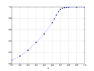
Fig. 1: Estimated convergence rate $r_{t}$ as a function of $\alpha$, with uniform time steps.

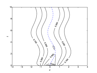
Fig. 2: Contour plot of the solution for the problem of Section 5.2. The dashed line shows the first moment $\bar{x}(t)$.

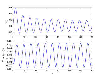
Fig. 3: Top: first moment (as computed via Laplace transforms) of the solution for the problem of Section 5.2. Bottom: error in the first moment of $U^{n}_{h}$.

In our first test problem, we considered (1) with

$$F(x,t)=x+\sin t,\quad T=1,\quad L=\pi,\quad\kappa_{\alpha}=\mu_{\alpha}=1,$$

where the source term $g$ was chosen so that $u(x,t)=[1+\omega_{1+\alpha}(t)]\sin x$. It follows that $u_{t}=O(t^{\alpha-1})$ as $t\to 0^{+}$, and this singular behaviour is known to be typical [12] for the fractional diffusion equation (that is, when the lower-order term in $F$ is absent). We employed a uniform spatial grid with $h=\pi/P$, but allowed a nonuniform spacing in time by putting

$$t_{n}=(n/N)^{\gamma}T,\quad\text{where $\gamma\geq 1$.}$$

Thus, $\gamma=1$ gives a uniform mesh with $k=T/N$, but if $\gamma>1$ then the time step is initially $k_{1}=T/N^{\gamma}=O(k^{\gamma})$ and increases monotonically up to a maximum of $k=k_{N}\approx\gamma T/N$. Such meshes [13] are commonly used to compensate for singular behaviour in the derivatives of $u$ at $t=0$. As a measure of the error in the numerical solution, we computed

$$E_{N,h}=\max_{0\leq n\leq N}\|U^{n}_{h}-u(t_{n})\|_{L_{2}(\Omega)},$$ (25)

(where the spatial $L_{2}$-norm was evaluated via Gauss quadrature) and sought to estimate the convergence rates $r_{t}$ and $r_{x}$ such that

$$E_{N,h}\approx C_{1}k^{r_{t}}+C_{2}h^{r_{x}},$$

from the relations

$$r_{t} \approx r_{t}(N,h)=\log_{2}(E_{N,h}/E_{2N,h}) h^{r_{x}}\ll k^{r_{t}}$$ when ,

$$r_{x} \approx r_{x}(N,h)=\log_{2}(E_{N,2h}/E_{N,h}) k^{r_{t}}\ll h^{r_{x}}$$ when .

We first tested the convergence behaviour with respect to the time discretization. Table 1 shows how $E_{N,h}$ varies with $N$, for a fixed, high-resolution spatial grid with $P=5120$ subintervals, when $\alpha=0.625$ and for three choices of $\gamma$. In the case of a uniform mesh ($\gamma=1$), we observe $r_{t}\approx 0.8$, suggesting that the $O(k^{\alpha})$ error bound of Theorem 15 is somewhat pessimistic in this case. Although the convergence analysis of our time-stepping scheme applies only when $\gamma=1$, we observe that $E_{N,h}\approx Ck$ if $\gamma\geq\alpha^{-1}=1.6$. (The constant $C$ is smallest when $\gamma=\alpha^{-1}$.) Table 2 shows results for three different choices of $\alpha$ as we vary $N$, using uniform time steps ($\gamma=1$) and the same fixed spatial grid as before. Note that the choices $\alpha=0.25$ and $\alpha=0.5$ are excluded by our theory, which requires $1/2<\alpha<1$. Figure 1 gives a more complete picture of the convergence rate $r_{t}$ as a function of $\alpha$ when $\gamma=1$, and may be compared with the known result $r_{t}=\min(2\alpha,1)$ for the homogeneous diffusion equation (that is, the special case $F=0$ and $g=0$) with regular initial data [14, Lemma 6].

Next, we tested how $E_{N,h}$ behaves as the spatial mesh is refined, using a fixed, high-resolution time discretization with $N=10,000$. Table 3 shows results for three different choices of $\alpha$ using a mesh grading $\gamma=\alpha^{-1}$ in each case. We see that $E(N,h)\approx C_{1}h^{2}$, consistent with Theorem 11 (when $1/2<\alpha<1$).

5.2 An application

In our second example, we solve the homogeneous equation on the spatial interval $(-L,L)$, that is,

$$u_{t}-\partial_{t}^{1-\alpha}u_{xx}+\bigl{(}F\partial_{t}^{1-\alpha}u\bigr{)}_{x}=0\quad\text{for $0<t<T$ and $-L<x<L$,}$$

with $F=-x+\sin t$, subject to the boundary conditions $u(\pm L,t)=0$. For the initial data $u_{0}$, we chose a normal probability density function with mean $0$ and variance $\sigma^{2}$. This choice of $F$ is taken from a recent paper by Angstmann et al. [1]; notice that $F_{x}=-1<0$ so the first assumption of Theorem 9 is not satisfied and we must rely on Theorem 10 to ensure stability of the spatially discrete scheme (6). For our computations, we used the values $\alpha=0.75$ and $\sigma=0.5$, with a mesh grading parameter $\gamma=1/\alpha$. Figure 2 shows a contour plot of the numerical solution computed using our fully discrete method in the case $L=9$, $T=10$, $N=100$ and $P=2L^{2}$. Although we do not know an analytical solution, Laplace transform techniques [1] show that in the limiting case when $L\to\infty$, and interpreting $u(\cdot,t)$ as a probability density function, the expected position, or first moment, is

$$\bar{x}(t)=\int_{-\infty}^{\infty}xu(x,t)\,dx=\frac{1}{\Gamma(\alpha)}\int_{0}^{t}E_{\alpha}\bigl{(}-(t-s)\bigr{)}s^{\alpha-1}\sin s\,ds,$$

where $E_{\alpha}$ denotes the Mittag–Leffler function (4). Figure 3 shows the oscillatory behaviour of $\bar{x}(t)$ for $0\leq t\leq T=70$, and the difference between this theoretical value and the first moment of the numerical solution $U^{n}_{h}$, in the case $L=20$, $N=20T$ and $P=2TL^{2}$. We observe little if any loss of accuracy over more than 10 oscillations.

5.3 Non-smooth initial data

In the special case of a fractional diffusion equation ($F\equiv 0$ and $g\equiv 0$), a standard energy argument shows that both the exact solution and the finite element solution are stable in $L_{2}(\Omega)$, with

$$\|u(t)\|\leq\|u_{0}\|\quad\text{and}\quad\|u_{h}(t)\|\leq\|u_{0h}\|\quad\text{for $t>0$.}$$

By comparison, for nonzero $F$ the stability estimates of Theorems 9 and 10 yield weaker bounds of the form

$$\|u_{h}(t)\|\leq C\|u_{0h}\|_{1}\quad\text{for $0\leq t\leq T$,}$$ (26)

and in the case of our (spatially continuous) time-stepping scheme, Theorem 14,

$$\|U^{n}\|\leq C\|U^{0}\|_{2}\quad\text{for $0\leq t\leq T$.}$$ (27)

To investigate whether the stability properties really depend on the smoothness of the initial data, we solved the same problem as in Section 5.2 but chose the nodal values for the discrete initial data $u_{0h}$ to be uniformly distributed pseudorandom numbers in the unit interval. For $0\leq t\leq T=40$ and many different combinations of $N$ and $P$, we never observed any kind of instability. In all cases, the solution quickly smoothed and began an oscillatory behaviour similar to that seen in Figure 2, suggesting that (26) and (27) are pessimistic with respect to the regularity required of the initial data.

Appendix A Positivity of discrete convolution operators

Recall the following positivity property of Fourier cosine series.

Lemma 16.

If the sequence $a_{0}$, $a_{1}$, $a_{2}$, …tends to zero and satisfies

$$a_{n}\geq 0\quad\text{and}\quad a_{n+1}\leq\tfrac{1}{2}(a_{n}+a_{n+2})\quad\text{for all $n\geq 0$,}$$

then

$$\frac{a_{0}}{2}+\sum_{n=1}^{\infty}a_{n}\cos n\theta\geq 0\quad\text{for $-\pi\leq\theta\leq\pi$.}$$

Proof.

Zygmund [20, p. 93 and Theorem (1.5), p. 183]. ∎

For $0<\alpha<1$, let

$$(AU)^{n}=\sum_{j=0}^{n}a_{n-j}U^{j}\quad\text{where $a_{n}=(n+1)^{\alpha}-n^{\alpha}$.}$$

We used the following inequality in the proof of Lemma 13.

Lemma 17.

For any real, square-summable sequence $U^{0}$, $U^{1}$, $U^{2}$, …,

$$\sum_{n=0}^{\infty}(AU)^{n}U^{n}\geq\frac{1}{2}\sum_{n=0}^{\infty}(U^{n})^{2}.$$

Proof. Define $\widetilde{V}(\theta)=\sum_{n=0}^{\infty}V^{n}e^{in\theta}$, and observe that

$$\int_{-\pi}^{\pi}\widetilde{U}(\theta)\overline{\widetilde{V}(\theta)}\,d\theta=\sum_{n=0}^{\infty}\sum_{j=0}^{\infty}U^{n}\overline{V^{j}}\int_{-\pi}^{\pi}e^{i(n-j)\theta}\,d\theta=2\pi\sum_{n=0}^{\infty}U^{n}\overline{V^{n}}.$$

Since

$$\widetilde{AU}(\theta)=\sum_{n=0}^{\infty}\biggl{(}\sum_{j=0}^{n}a_{n-j}U^{j}\biggr{)}e^{in\theta}=\sum_{j=0}^{\infty}\biggl{(}\sum_{n=j}^{\infty}a_{n-j}e^{i(n-j)\theta}\biggr{)}U^{j}e^{ij\theta}=\tilde{a}(\theta)\widetilde{U}(\theta)$$

we conclude

$$\sum_{n=0}^{\infty}(AU)^{n}\overline{V^{n}}=\frac{1}{2\pi}\int_{-\pi}^{\pi}\tilde{a}(\theta)\widetilde{U}(\theta)\overline{\widetilde{V}(\theta)}\,d\theta.$$

In particular, when $V^{n}=U^{n}$ is purely real,

$$\sum_{n=0}^{\infty}(AU)^{n}U^{n}=\frac{1}{2\pi}\int_{-\pi}^{\pi}\Re\tilde{a}(\theta)|\widetilde{U}(\theta)|^{2}\,d\theta.$$

The function $f(x)=(x+1)^{\alpha}-x^{\alpha}$ is positive for $x\geq 0$, and as $x\to\infty$,

$$f(x)=x^{\alpha}[(1+x^{-1})^{\alpha}-1]=x^{\alpha}[\alpha x^{-1}+O(x^{-2})]=\alpha x^{\alpha-1}+O(x^{\alpha-2}),$$

so in particular $f(x)\to 0$. Furthermore, $f$ is convex because

$$f^{\prime\prime}(x)=\alpha(\alpha-1)\bigl{[}(x+1)^{\alpha-2}-x^{\alpha-2}\bigr{]}=\alpha(1-\alpha)\bigl{[}x^{\alpha-2}-(x+1)^{\alpha-2}\bigr{]}\geq 0$$

for all $x>0$, so the sequence $a_{n}=f(n)$ satisfies the assumptions of Lemma 16. Hence, $\Re\tilde{a}(\theta)\geq a_{0}/2=1/2$ and finally

$$\sum_{n=0}^{\infty}(AU)^{n}U^{n}\geq\frac{1}{2\pi}\int_{-\pi}^{\pi}\frac{1}{2}|\widetilde{U}(\theta)|^{2}\,d\theta=\frac{1}{2}\sum_{n=0}^{\infty}(U^{n})^{2}.\qquad\end@proof$$

References

- [1] C. N. Angstmann, I. C. Donnelly, B. I. Henry, T. A. M. Langlands, and P. Straka, Generalised continuous time random walks, master equations and fractional Fokker–Planck equations, SIAM J. Appl. Math., 75 (2015), pp. 1445–1468.
- [2] Leigh C. Becker, Resolvents and solutions of weakly singular linear Volterra integral equations, Nonlinear Analysis, 74 (2011), pp. 1892–1912.
- [3] X. N. Cao, J.-L. Fu, and H. Huang, Numerical method for the time fractional Fokker–Planck equation, Adv. Appl. Math. Mech., 4 (2012), pp. 848–863.
- [4] S. Chen, F. Liu, P. Zhuang, and V. Anh, Finite difference approximations for the fractional Fokker–Planck equation, Appl. Math. Model., 33 (2009), pp. 256–273.
- [5] Mingrong Cui, Compact exponential scheme for the time fractional convection-diffusion reaction equation with variable coefficients, J. Comput. Phys., 280 (2015), pp. 143–163.
- [6] Weihua Deng, Numerical algorithm for the time fractional Fokker–Planck equation, J. Comput. Phys., 227 (2007), pp. 1510–1522.
- [7] J. Dixon and S. McKee, Weakly singular Gronwall inequalities, ZAMM Z. Angew. Math. Mech., 66 (1986), pp. 535–544.
- [8] G. Fairweather, H. Zhang, X. Yang, and D. Xu, A backward Euler orthogonal spline collocation method for the time-fractional Fokker–Planck equation, Numer. Meth. PDEs. Published online 28 December, 2014.
- [9] E. Heinsalu, M. Patriarca, I. Goychuk, and P. Hänggi, Use and abuse of a fractional Fokker–Planck dynamics for time-dependent driving,, Phys. Rev. Lett., 99 (2007), p. 120602.
- [10] B. I. Henry, T. A. M. Langlands, and P. Straka, Fractional Fokker–Planck equations for subdiffusion with space- and time-dependent forces, Phys. Rev. Lett., 105 (2010), p. 170602.
- [11] Yingjun Jiang, A new analysis of stability and convergence for finite difference schemes solving the time fractional Fokker–Planck equation, Appl. Math. Model., 39 (2015), pp. 1163–1171.
- [12] William McLean, Regularity of solutions to a time-fractional diffusion equation, ANZIAM J., 52 (2010), pp. 123–138.
- [13] William McLean and Kassem Mustapha, Convergence analysis of a discontinuous Galerkin method for a sub-diffusion equation, Numer. Algor., 52 (2009), pp. 69–88.
- [14] , Time-stepping error bounds for fractional diffusion problems with non-smooth initial data, J. Comput. Phys., 293 (2015), pp. 201–217.
- [15] R. Metzler, E. Barkai, and J. Klafter, Deriving fractional Fokker–Planck equations from a generalised master equation, Europhys. Lett., 46 (1999), pp. 431–436.
- [16] Kassem Mustapha and Dominik Schötzau, Well-posedness of -version discontinuous Galerkin methods for fractional diffusion wave equations, IMA J. Numer. Anal., 34 (2014), pp. 1426–1446.
- [17] Abbas Saadatmandi, Mehdi Dehghan, and Mohammad-Reza Azizi, The Sinc–Legendre collocation method for a class of fractional convection–diffusion equations with variable coefficients, Commun. Nonlinear Sci. Numer. Simul., 17 (2012), pp. 4125–4136.
- [18] Seakweng Vong and Zhibo Wang, A high order compact finite difference scheme for time fractional Fokker–Planck equations, Appl. Mat. Lett., 43 (2015).
- [19] Haiping Ye, Jianming Gao, and Yongsheng Ding, A generalized Gronwall inequality and its application to a fractional differential equation, J. Math. Anal. Appl., 328 (2007), pp. 1075–1081.
- [20] Antoni Zygmund, Trigonometric Series, vol. I, Cambridge University Press, 1959.