Antisymmetric galaxy cross-correlations as a cosmological probe

Abstract

The auto-correlation between two members of a galaxy population is symmetric under the interchange of the two galaxies being correlated. The cross-correlation between two different types of galaxies, separated by a vector $\mathbf{r}$, is not necessarily the same as that for a pair separated by $-\mathbf{r}$. Local anisotropies in the two-point cross-correlation function may thus indicate a specific direction which when mapped as a function of position trace out a vector field. This vector field can then be decomposed into longitudinal and transverse components, and those transverse components written as positive- and negative-helicity components. A locally asymmetric cross-correlation of the longitudinal type arises naturally in halo clustering, even with Gaussian initial conditions, and could be enhanced with local-type non-Gaussianity. Early-Universe scenarios that introduce a vector field may also give rise to such effects. These antisymmetric cross-correlations also provide a new possibility to seek a preferred cosmic direction correlated with the hemispherical power asymmetry in the cosmic microwave background and to seek a preferred location associated with the CMB cold spot. New ways to seek cosmic parity breaking are also possible.

I Introduction

Considerable evidence has accrued for the past decade that large-scale structure in the Universe grew via gravitational infall from a nearly scale-invariant spectrum of very nearly Gaussian primordial adiabatic density perturbations Bennett:2012zja ; Ade:2015xua . The nature of these perturbations is generally accounted for in terms of single-field slow-roll (SFSR) inflation inflation . However, even if SFSR is the correct explanation, there might be new physics beyond SFSR inflation, and there remains the ever-present possibility that primordial perturbations are due to something completely different.

In order to develop a clearer understanding of the new physics responsible for primordial perturbations, we must be vigilant in seeking new fossils from the early Universe in the form of subtle correlations in the matter distribution. This is the motivation for much of the work on non-Gaussianity Bartolo:2004if . This Letter will explore new observables that can be sought with galaxy surveys. Such work is timely given the advent in the forthcoming years of a new generation of surveys Ivezic:2008fe ; Maartens:2015mra ; Green:2012mj ; Laureijs:2011gra that will map the distribution of galaxies over vast volumes in the Universe.

Recent work Jeong:2012df presented a parametrization of the most general autocorrelation function—which may depend on the orientation of the two points being correlated as well as their position in space—and showed that it could be decomposed into scalar, vector, and tensor components. Here we generalize that work to the most general two-point cross-correlation function between two different galaxy populations. If primordial perturbations are Gaussian, then the two-point correlation function is statistically isotropic and homogeneous. More generally, though, the two-point correlation function may, at least in some small region of space, be anisotropic. That anisotropy may also vary from one point in the Universe to another. Ref. Jeong:2012df parametrized the most general local departure from isotropy for an auto-correlation function. Since an auto-correlation function for two galaxies separated by a vector $\mathbf{r}$ must be invariant under the inversion $\mathbf{r}\to-\mathbf{r}$, the most general departure from statistical isotropy is parametrized in terms of a symmetric tensor, or more generally, in terms of the six degrees of freedom that parametrize that tensor.

If, however, we consider the two-point cross-correlation function between two distinct populations, then it is possible that the correlation function for a galaxy pair separated by $\mathbf{r}$ may differ from that with separation $-\mathbf{r}$. There is thus a possibility that the two-point correlation function might “point” in a given direction, and this pointing is described by a vector. Our purpose here is to point out that evidence of the imprint of a vector field can be sought with cross-correlatoins in the galaxy distribution. Our work differs from that of Refs. Bonvin:2013ogt ; McDonald:2009ud ; Yoo:2012se , who also considered asymmetric galaxy cross-correlations; while they considered only those that arise from projection effects, we consider bona fide asymmetries in the three-dimensional distribution. Since observations are done in redshift space, though, care must be taken to disentangle the 3D asymmetries we consider below from the redshift-space asymmetries discussed in Refs. Bonvin:2013ogt ; McDonald:2009ud ; Yoo:2012se , and from the angular dependence induced by the 3D RSD operator Raccanelli:3D .

Below we describe the parametrization of the most general two-point cross-correlation, beginning by reprising the parameterization for the auto-correlation function. We then discuss the decomposition of these types of local departures from statistical isotropy in terms of two transverse and one longitudinal mode. Next, we write down the optimal quadratic estimators to be constructed from galaxy surveys to detect these departures from statistical isotropy. After that, we discuss several possible physical mechanisms to generate these types of local departures from statistical isotropy. We begin this discussion with an effect that arises in biased halo clustering, even with Gaussian initial conditions, and another that arises in halo clustering if there is local-type primordial non-Gaussianity. We then describe several early-Universe scenarios for such correlations. We point out that a search for these anisotropic cross-correlations may be used to seek a preferred cosmic direction correlated with the direction indicated by the hemispherical power asymmetry Eriksen:2003db ; Ade:2013nlj or to seek a preferred location associated with the CMB cold spot Vielva . Finally, we mention the possibliity to construct new probes of parity breaking.

II Parametrization of the cross-correlation

We begin by reprising the parametrization of Ref. Jeong:2012df for the two-point auto-correlation function. Suppose we have a density field $\delta(\mathbf{x})$ from which we construct the Fourier components $\delta(\mathbf{k})$. The most general two-point correlation function for those Fourier components can be parametrized as,

$$\left\langle\delta(\mathbf{k}_{1})\delta(\mathbf{k}_{2})\right\rangle = P(k_{1})\delta_{\mathbf{k}_{1},-\mathbf{k}_{2}}+\sum_{\mathbf{K}}\sum_{p}f_{p}(k_{1},k_{2},\mu)$$ (1)

$$\times h_{p}^{*}(\mathbf{K})\epsilon_{ij}^{p}(\mathbf{K})k_{1}^{i}k_{2}^{j}\,\delta^{D}_{\mathbf{k}_{123}},$$

where $\delta_{\mathbf{k}_{1},-\mathbf{k}_{2}}$ is a Kronecker delta, and $\delta^{D}_{\mathbf{k}_{123}}$ is a Kronecker delta that sets $\mathbf{k}_{1}+\mathbf{k}_{2}+\mathbf{K}=0$. Here $p$ sums over the six possible basis tensors for a symmetric tensor, and $\epsilon_{ij}^{p}(\mathbf{K})$ are the six polarization tensors which can be written as a trace, a longitudinal mode, two transverse-vector modes, and two transverse traceless tensor modes. The $h_{p}(\mathbf{K})$ are Fourier amplitudes of the various types of perturbations, and $f_{p}(k_{1},k_{2},\mu)$ parametrizes the dependence on $\mathbf{k}_{1}$ and $\mathbf{k}_{2}$ (where $\mu$ is the cosine of the angle between $\mathbf{k}_{1}$ and $\mathbf{k}_{2}$). The first term in Eq. (1) indicates the statistically isotropic correlation with power spectrum $P(k)$. It was argued in Ref. Jeong:2012df , simply from symmetry considerations (and in particular, the dependence of the correlation on the azimuthal angle about the direction of $\mathbf{K}$), that terms with the two scalar, the two vector, or the two tensor polarizations can arise in inflation if the inflaton is coupled to a new scalar, vector, or tensor field, respectively.

Our purpose here, though, is to consider the additional possibility that arises when we cross-correlate two different tracers of the matter distribution. The fractional density perturbations of these two populations will have Fourier amplitudes $\delta_{1}(\mathbf{k}_{1})$ and $\delta_{2}(\mathbf{k}_{2})$, respectively. The most general two-point correlations of these Fourier coefficients will satisfy a relation like Eq. (1), but the sum on $p$ will now be extended from six to nine to account for the three possibilities where $\epsilon^{p}_{ij}(\mathbf{K})$ is antisymmetric. The three new degrees of freedom in the cross-correlation, not allowed with auto-correlations, can be written most generally, for $\mathbf{k}_{1}\neq-\mathbf{k}_{2}$, as,

$$\left\langle\delta_{1}(\mathbf{k}_{1})\delta_{2}(\mathbf{k}_{2})\right\rangle=\sum_{\mathbf{K},p}f_{p}\left(\mathbf{k}_{1},\mathbf{k}_{2},\mu\right)h_{p}^{*}(\mathbf{K})\hat{\epsilon}_{p}\cdot\left(\mathbf{k}_{1}-\mathbf{k}_{2}\right)\delta^{D}_{\mathbf{k}_{123}}.$$ (2)

Here, the sum on $p$ runs over the three polarizations $p=L,x,y$, where $\hat{\epsilon}_{L}(\mathbf{K})=\hat{K}$ and $\epsilon_{x,y}(\mathbf{K})$ are two other unit vectors orthogonal to $\hat{K}$ and to each other. Just from symmetry considerations, we expect that correlations with $p=L$ could arise if there is some longitudinal-vector field—or equivalently, the scalar field from which it is derived—coupled to whatever physics determines the galaxy distribution. Similarly, distortions with $p=x,y$ would require that the galaxy distribution was determined, at least in part, by some transverse-vector field.

Eq. (2) describes, in Fourier space, cross-correlations between two different populations, that are antisymmetric in the exchange of the two populations. In configuration space, these correlations trace out a vector field, as follows: In any small volume of the Universe, the cross-correlation could “point” in some given direction; i.e., there could be a mean offset between galaxies of type 1 (e.g., more massive galaxies) and galaxies of type 2 (e.g., less massive galaxies). This thus implies a preferred direction in that volume. The generality of the parametrization in Eq. (2) allows for the possibility that this preferred direction is spatially dependent in such a way that global statistical isotropy is preserved on sufficiently large scales. It also allows for the possibility, though, for a preferred direction across the entire observable Universe. This latter possibility clearly requires some exotic new physics, but the imprint of a local preferred direction is not at all exotic, as we will see.

III Estimators

We now describe how to measure these vectorial cross-correlations from a galaxy survey. We will consider the longitudinal and transverse components separately and begin with longitudinal distortions, supposing that $f_{L}(k_{1},k_{2},\mu)$ is specified. Suppose further that the physical model specifies that the Fourier components $h_{L}(\mathbf{K})$ are selected from a Gaussian distribution with power spectrum $P_{L}(K)=A_{L}P_{L}^{f}(K)$ of amplitude $A_{L}$ and fiducial $K$ dependence $P_{L}^{f}(k)$. Following the same steps as in Ref. Jeong:2012df , the optimal estimator for the amplitude $A_{L}$ is given by

$$\widehat{A_{L}}=\sigma_{L}^{2}\sum_{\mathbf{K}}\frac{P_{L}^{f}(K)}{2\left[P_{L}^{n}(K)\right]^{2}}\left(V^{-1}\left|\widehat{h_{L}(\mathbf{K})}\right|^{2}-P_{L}^{n}(K)\right),$$ (3)

and this amplitude is determined with inverse variance,

$$\sigma_{L}^{-2}=(1/2)\sum_{\mathbf{K}}\left[P_{L}^{f}(K)\right]^{2}\left[P_{L}^{n}(K)\right]^{-2}.$$ (4)

Here,

$$\widehat{h_{L}(\mathbf{K})} = P_{L}^{n}(K)\sum_{\mathbf{k}}\frac{f_{L}\left(k,|\mathbf{K}-\mathbf{k}|,\mu\right)\hat{K}\cdot(\mathbf{K}+2\mathbf{k})}{2VP_{1}^{\rm tot}(k)P^{\rm tot}_{2}(|\mathbf{K}-\mathbf{k}|)}$$ (5)

$$\ \ \ \ \times\delta_{1}(\mathbf{k})\delta_{2}(\mathbf{K}-\mathbf{k}),$$

is the estimator for the amplitude $h_{L}(\mathbf{K})$, where here $\mu=\hat{k}\cdot(\mathbf{K}-\mathbf{k})$, and the noise power spectrum for $\widehat{h_{L}(\mathbf{K})}$ is

$$P_{L}^{n}(K)=\left[\sum_{\mathbf{k}}\frac{\left|f_{L}\left(k,|\mathbf{K}-\mathbf{k}|,\mu\right)\hat{K}\cdot(\mathbf{K}+2\mathbf{k})\right|^{2}}{2VP^{\rm tot}_{1}(k)P^{\rm tot}_{2}\left(|\mathbf{K}-\mathbf{k}|\right)}\right]^{-1}.$$ (6)

In these expressions, $V$ is the volume of the survey, the sums are over the wavenumbers $\mathbf{k}$ for which the density perturbations are measured; $P_{1}(K)$ and $P_{2}(K)$ are the power spectra for the two populations; and $P^{\rm tot}$ is the total power spectrum, the sum of the signal and the shot noise. If instead we consider distortions of the transverse-vector type, then the optimal estimator for the amplitude $A_{T}$ for the power spectrum for the transverse-vector field will be as above, but with $\hat{K}$ replaced by $\hat{\epsilon}_{i}({\mathbf{K}})$ and an additional sum over the two transverse polarizations.

IV Sources of asymmetric galaxy cross-correlations

IV.1 Biased halo clustering

We now show that asymmetric cross-correlations arise in the standard model for biased halo clustering from Gaussian initial conditions. Let $\delta(\mathbf{x})$ be the primordial fractional mass-density perturbation, and suppose that this density field is populated by two different types of halos. These could be, for example, high-mass halos (e.g., those that house giant ellipticals, clusters, etc.) and low-mass halos (e.g., those that house Milky-Way type galaxies, dwarf galaxies, etc.). Let $n_{1}(\mathbf{x})$ be the fractional perturbation in the number density, as a function of position $\mathbf{x}$, of halos of type 1 and similarly for $n_{2}(\mathbf{x})$. Since the abundance of halos in some region is a nonlinear function of the local mass density, there are nonlinear relations Fry:1992vr , $n_{1}(\mathbf{x})=b_{1}\delta(\mathbf{x})+c_{1}[\delta(\mathbf{x})]^{2}+\cdots$ and $n_{2}(\mathbf{x})=b_{2}\delta(\mathbf{x})+c_{2}[\delta(\mathbf{x})]^{2}+\cdots$ between the halo and mass densities, where $b_{1}$ and $b_{2}$ are the usual linear-bias parameters, and $c_{1}$ and $c_{2}$ are nonlinear-bias parameters. The nonlinear relation between $n_{i}$ and $\delta(\mathbf{x})$ implies that there will be a three-point correlation,

(7)

If we antisymmetrize in $\mathbf{k}_{1}$ and $\mathbf{k}_{2}$, we find an antisymmetric part, $\propto 2P(K)(b_{2}c_{1}-b_{1}c_{2})\left[P(k_{1})-P(k_{2})\right]$ to this three-point function. We now consider the squeezed limit, $\mathbf{k}\equiv\mathbf{k}_{1}\sim-\mathbf{k}_{2}$ and $k\simeq k_{1},k_{2}\gg K$, appropriate if we are considering the small-scale clustering of halos in the presence of a low-pass-filtered density field. The part of the bispectrum antisymmetric in $\mathbf{k}_{1}$ and $\mathbf{k}_{2}$ is then $2(b_{1}c_{2}-b_{2}c_{1})P(K)[dP(k)/dk]\mathbf{K}\cdot\hat{\mathbf{k}}$. We thus see that in the presence of a long-wavelength mode of $\delta(\mathbf{x})$, the high-pass-filtered $n_{1}(\mathbf{x})$ and $n_{2}(\mathbf{x})$ have a Fourier-space cross-correlation precisely of the form in Eq. (2) with $f_{L}=[dP(k)/dk](b_{1}c_{2}-b_{2}c_{1})(K/k)$. The longitudinal, rather than transverse, mode is as expected in the presence of the long-wavelength density perturbation.

Existing measurements Verde:2001sf ; Gil-Marin:2014sta ; Marin:2013bbb ; McBride:2010zn ; Marin:2010iv of nonlinear-bias parameters from galaxy bispectra Fry:1994my ; Matarrese:1997sk ; Buchalter:1999vc have relied entirely on measurement of auto-correlations. Cross-correlations have also been used to infer bias parameters Croft:1998wq ; Martinez:1998be ; Knobel:2012xb ; Shen:2012rr , but those works considered only the linear bias. If a galaxy sample is broken up into two different populations, the linear- and nonlinear-bias parameters for the two populations can be measured with the bispectra for the two different populations. The symmetric part of the cross-correlation between these two populations then provides a measurement of the combination $b_{1}c_{2}+b_{2}c_{1}$, and the antisymmetric part of this cross-correlation provides $b_{2}c_{1}-b_{1}c_{2}$. The latter provides some incremental improvement in statistical power, and it can also complement other measurements of the bias parameters and be used to check the validity of the biasing-model assumptions behind the analyses. Indeed, from Eq. (7) and what follows, we see that for a power-law $P(k)$, the ratio between the symmetric and asymmetric signals is $\propto(b_{2}c_{1}-b_{1}c_{2})K/2(b_{1}c_{2}+b_{2}c_{1})k$, which is generically small in the squeezed limit $k\gg K$. However, for populations with negative non-linear bias on certain scales (see e. g. Pollack:2013alj ), it is certainly possible that the bias parameters contrive to yield $b_{1}c_{2}+b_{2}c_{1}\approx 0$, in which case the asymmetric information becomes particularly beneficial.

IV.2 Primordial non-Gaussianity

Asymmetry may arise even with linear biasing if there is primordial non-Gaussianity of the local type. In this case, the linear-bias parameters for the two halo populations may be scale dependent, $n_{1}(\mathbf{k}_{1})=b_{1}(k_{1})\delta(\mathbf{k}_{1})$ and $n_{2}(\mathbf{k}_{2})=b_{2}(k_{2})\delta(\mathbf{k}_{2})$. Here $b_{i}(k)\approx b_{i}+2(b_{i}-1)\delta_{c}{f_{\rm nl}}\Omega_{m}3(aH/k)^{2}/2$ with the standard scale-independent bias $b_{i}$ and some collapse threshold $\delta_{c}$ Dalal:2007cu ; Matarrese:2008nc ; Schmidt:2010gw . On the other hand, the matter-density perturbation is expected to develop a nonzero bispectrum $B(k_{1},k_{2},K)$ due to nonlinear gravitational growth Fry:1983cj ; Goroff:1986ep ; Kamionkowski:1998fv (this should not be confused with the primordial bispectrum). The three-point function $\left\langle n_{1}(\mathbf{k}_{1})n_{2}(\mathbf{k}_{2})\delta(\mathbf{K})\right\rangle\propto b_{1}(k_{1})b_{2}(k_{2})B(k_{1},k_{2},K)$ is thus noninvariant if we exchange $\mathbf{k}_{1}$ and $\mathbf{k}_{2}$, and we again recover an antisymmetric correlation $\propto\left[b_{1}(k_{1})b_{2}(k_{2})-b_{1}(k_{2})b_{2}(k_{1})\right]B(k_{1},k_{2},K)/P(K)$, with

$$f_{L}=3(b_{1}-b_{2})\delta_{c}{f_{\rm nl}}\Omega_{m}\frac{(aH)^{2}K}{k_{1}^{2}k_{2}^{2}}\frac{B(k_{1},k_{2},K)}{P(K)}.$$ (8)

IV.3 Primordial longitudinal vector field

We now describe an exotic scenario that could give rise to an anisotropic two-point correlation. Consider a curvaton-like inflation model in which primordial density perturbations are due not to fluctuations in the inflaton, but to fluctuations in some spectator field. Suppose further that this curvaton-like field is complex and coupled to a new $U(1)$ gauge field. There will then be charge-density fluctuations that arise during inflation, and if the $U(1)$ symmetry is broken after inflation, those charge-density fluctuations may survive. It is then conceivable that dark matter may be like baryonic matter in our Universe, in which there are light electron-like dark-matter particles and heavier proton-like dark-matter particles of opposite charge. If so, then galaxies that form in regions with a positive charge-density fluctuation may be different than those that form in regions with negative charge-density fluctuations. The cross-correlations between these two different types of galaxies—which for example may appear to us as brighter or fainter galaxies—should then trace out the large-scale electric-type field associated with the early-Universe $U(1)$ gauge field (see Fig. 1). Such a longitudinal-type cross-correlation could in principle be distinguished from that due to halo clustering from the different dependences on $\mathbf{k}$. Unlike the halo-biasing case, in which small-scale directionality indicated by anisotropic cross-correlations are correlated with the long-wavelength density field, these anisotropic correlations would have no cross-correlation with the large-scale density field.

IV.4 Primordial transverse vector field

What about anisotropic cross-correlations of the transverse variety? As we have seen above, modulation of small-scale galaxy-density fluctuations by a long-wavelength density mode arise naturally, but those are of the longitudinal variety. Any small-scale anisotropic cross-correlation that traced out a transverse-vector field would thus provide clear indication of new physics. There are indeed a number of inflationary scenarios that involve new vector fields vectors and models of gravity in which the vector degrees of freedom in the metric are brought to life Hellings:1973zz , and it is reasonable to surmise that one of these provide an imprint of the type we consider. To see how this may work, suppose the inflaton (or curvaton) $\phi$ is coupled to a vector field $A^{\mu}$ through a term $\partial^{(\mu}A^{\nu)}(\partial_{\mu}\phi)(\partial_{\nu}\phi)$, where the parentheses in the superscripts indicate symmetrization (antisymmetrization would make this term vanish). Although the coupling of a mode of wavenumber $\mathbf{K}$ of the vector field to two scalar-field modes of wavevectors $\mathbf{k}_{1}$ and $\mathbf{k}_{2}$ would be symmetric under $\mathbf{k}_{1}\leftrightarrow\mathbf{k}_{2}$, one could again construct a model with two dark-matter components, sourcing two different galaxy populations in the respective dark matter halos made up from each component, in a way that makes the cross-correlation in one of the transverse directions asymmetric (see illustration in Fig. 1). These transverse-vector cross-correlations will be straightforward to measure with a galaxy survey and any non-null result would be extraordinarily interesting. The measurement will also be useful as a unique null test for systematic effects.

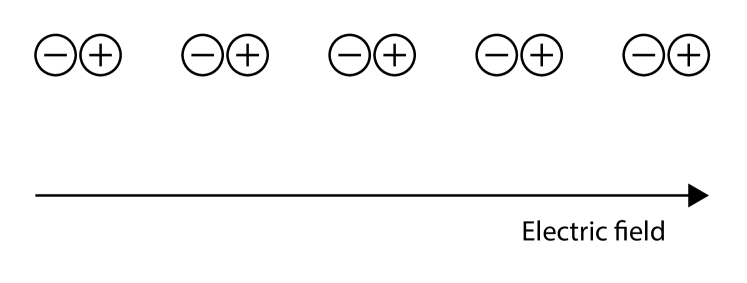
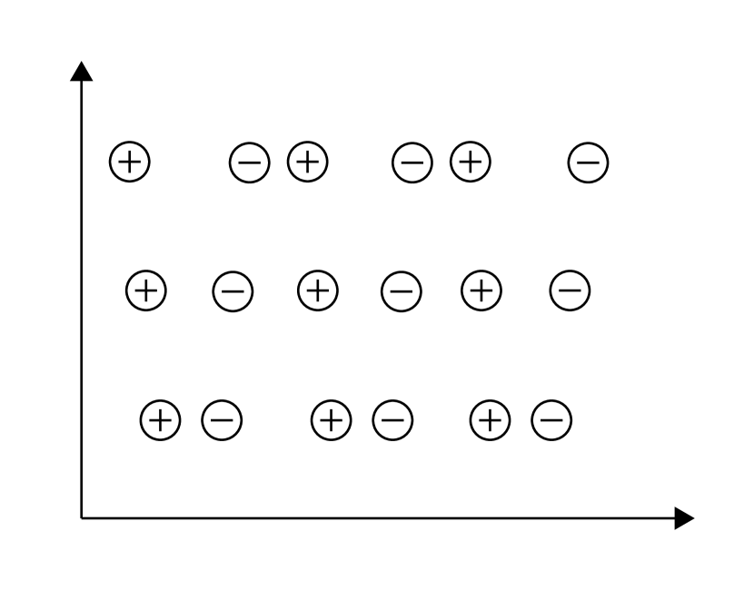
Figure 1: We consider models with two components of dark matter with some dipole interaction. Top: An “electric field” in the longitudinal direction leads to the arrangement in the pattern shown above. Then at the separation scale corresponding to the distance between “-” and “+”, there is an asymmetric cross-correlation between the “-” and “+” populations, along this longitudinal direction. The estimators derived in this work are designed to detect such a transverse vector asymmetry. Botom: A different setup, for which the asymmetry has a sinusoidal modulation in the transverse direction, leading to a transverse asymmetric cross-correlation.

IV.5 The CMB power asymmetry and cold spot

There is evidence for a hemispherical power asymmetry in the cosmic microwave background Eriksen:2003db ; Ade:2013nlj and it is important to investigate whether this preferred direction shows up anywhere else. If the CMB power asymmetry is due to the long-wavelength modulation of primordial perturbations Prunet:2004zy ; Gordon:2005ai ; Gordon:2006ag ; Erickcek:2008sm ; Erickcek:2009at ; Dai:2013kfa , then anisotropic cross-correlation of the type discussed above for biased halo clustering should exist, but with just one long-wavelength mode $h_{L}(\mathbf{K})$ of wavenumber $\mathbf{K}\to 0$ in the direction of the CMB power asymmetry. In simple terms, this Fourier amplitude $h_{L}(\mathbf{K})$ seeks whether a less massive galaxy is more likely to be found on one side of a more massive galaxy than on the other side.

Measurements from Planck Ade:2013nlj ; Ade:2015hxq also confirm the existence of a cold spot in the CMB Vielva . An asymmetric cross-correlation that traces out a hedgehog configuration surrounding the cold spot could conceivably arise either from a large void Inoue:2006rd or from exotic physics Turok:1990gw that may be responsible for the cold spot. A template for such a configuration could be constructed from the estimators $\widehat{h_{L}(\mathbf{K})}$ discussed above.

IV.6 Parity breaking?

There are also novel probes of cosmic parity breaking that can be constructed. Estimators for the two transverse modes $h_{p}(\mathbf{K})$ for each wavevector $\mathbf{K}$ can be constructed analogously to Eq. (5) by replacing the vector $\mathbf{K}$ that appears in the dot product with one of the two transverse polarization vectors. Those two linear polarization vectors $\hat{\epsilon}_{x}$ and $\hat{\epsilon}_{y}$ can be replaced by circular polarizations $\hat{\epsilon}_{\pm}(\mathbf{K})=2^{-1/2}[\epsilon_{x}(\mathbf{K})\pm i\epsilon_{y}(\mathbf{K})]$. Estimators for the Fourier amplitudes of these helicity states are then given by

$$\widehat{h_{\pm}(\mathbf{K})} = P_{L}^{n}(K)\sum_{\mathbf{k}}\frac{f_{L}\left(k,|\mathbf{K}-\mathbf{k}|,\mu\right)\hat{\mathbf{\epsilon}}_{\pm}\cdot(\mathbf{K}+2\mathbf{k})}{2VP_{1}^{\rm tot}(k)P^{\rm tot}_{2}(|\mathbf{K}-\mathbf{k}|)}$$ (9)

$$\ \ \ \ \times\delta_{1}(\mathbf{k})\delta_{2}(\mathbf{K}-\mathbf{k}).$$

It is then straightforward, following the power-spectrum-amplitude estimators discussed above, to construct estimators to check for an asymmetry between the power in right and left circularly polarized modes. Again, while a null result would not be too surprising, a positive result, if found, would be revolutionary.

V Conclusions

We have shown that cross-correlations between different galaxy populations may “point” in a given direction. The vector field from this pointing can be reconstructed from galaxy clustering, and it can be decomposed into longitudinal and transverse components, and also into components of positive and negative helicity. We discussed several physical mechanisms that may give rise to these departures from local statistical isotropy. These include nonlinear halo biasing, an effect that should arise in the standard model of halo clustering, and local-type non-Gaussian primordial perturbations. Other possiblities include couplings of the primordial field responsible for primordial perturbations to a new vector field, as well as a coupling to some field that might account for the hemispherical power asymmetry or cold spot in the CMB. The clustering effects from halo biasing constitute concrete predictions of the standard halo-clustering model that can be measured and used to test that standard model. Although the exotic possibilities we discussed are long shots, they will be easily sought in forthcoming surveys and would, if discovered, be quite remarkable.

Acknowledgments. MK acknowledges the hospitality of the Aspen Center for Physics, supported by NSF Grant No. 1066293. This work was supported at JHU by NSF Grant No. 0244990, NASA NNX15AB18G, the John Templeton Foundation, and the Simons Foundation. MS was supported in part by a Grant-in-Aid for JSPS Research under Grant No. 27-10917, and in part by World Premier International Research Center Initiative (WPI Initiative), MEXT, Japan.

References

- (1) C. L. Bennett et al. [WMAP Collaboration], Astrophys. J. Suppl. 208, 20 (2013) [arXiv:1212.5225 [astro-ph.CO]].
- (2) P. A. R. Ade et al. [Planck Collaboration], arXiv:1502.01589 [astro-ph.CO].
- (3) A. H. Guth and S. Y. Pi, Phys. Rev. Lett. 49, 1110 (1982); A. A. Starobinsky, Phys. Lett. B 117, 175 (1982); J. M. Bardeen, P. J. Steinhardt and M. S. Turner, Phys. Rev. D 28, 679 (1983); V. F. Mukhanov and G. V. Chibisov, JETP Lett. 33, 532 (1981) [Pisma Zh. Eksp. Teor. Fiz. 33, 549 (1981)]; S. W. Hawking, Phys. Lett. B 115, 295 (1982); A. D. Linde, Phys. Lett. B 116, 335 (1982).
- (4) N. Bartolo, E. Komatsu, S. Matarrese and A. Riotto, Phys. Rept. 402, 103 (2004) [astro-ph/0406398].
- (5) Z. Ivezic et al. [LSST Collaboration], arXiv:0805.2366 [astro-ph].
- (6) R. Maartens et al. [SKA Cosmology SWG Collaboration], PoS AASKA 14, 016 (2015) [arXiv:1501.04076 [astro-ph.CO]].
- (7) J. Green, P. Schechter, C. Baltay, R. Bean, D. Bennett, R. Brown, C. Conselice and M. Donahue et al., arXiv:1208.4012 [astro-ph.IM].
- (8) R. Laureijs et al. [EUCLID Collaboration], arXiv:1110.3193 [astro-ph.CO].
- (9) D. Jeong and M. Kamionkowski, Phys. Rev. Lett. 108, 251301 (2012) [arXiv:1203.0302 [astro-ph.CO]].
- (10) C. Bonvin, L. Hui and E. Gaztanaga, Phys. Rev. D 89, 083535 (2014) [arXiv:1309.1321 [astro-ph.CO]].
- (11) P. McDonald, JCAP 0911, 026 (2009) [arXiv:0907.5220 [astro-ph.CO]].
- (12) J. Yoo, N. Hamaus, U. Seljak and M. Zaldarriaga, Phys. Rev. D 86, 063514 (2012) [arXiv:1206.5809 [astro-ph.CO]].
- (13) A. Raccanelli, D. Bertacca, O. Doré and R. Maartens, JCAP 1408, 022 (2014) [arXiv:1306.6646 [astro-ph.CO]].
- (14) H. K. Eriksen, F. K. Hansen, A. J. Banday, K. M. Gorski and P. B. Lilje, Astrophys. J. 605, 14 (2004) [Astrophys. J. 609, 1198 (2004)] [astro-ph/0307507].
- (15) P. A. R. Ade et al. [Planck Collaboration], Astron. Astrophys. 571, A23 (2014) [arXiv:1303.5083 [astro-ph.CO]].
- (16) P. A. R. Ade et al. [Planck Collaboration], arXiv:1506.07135 [astro-ph.CO].
- (17) P. Vielva et al., Astrophys. J. 609, 22 (2004) [astro-ph/0310273]; M. Cruz et al., Mon. Not. Roy. Astron. Soc. 356, 29 (2005) [astro-ph/0405341].
- (18) J. N. Fry and E. Gaztanaga, Astrophys. J. 413, 447 (1993) [astro-ph/9302009].
- (19) L. Verde, A. F. Heavens, W. J. Percival, S. Matarrese, C. M. Baugh, J. Bland-Hawthorn, T. Bridges and R. Cannon et al., Mon. Not. Roy. Astron. Soc. 335, 432 (2002) [astro-ph/0112161].
- (20) H. Gil-Marín, J. Noreña, L. Verde, W. J. Percival, C. Wagner, M. Manera and D. P. Schneider, Mon. Not. Roy. Astron. Soc. 451, 5058 (2015) [arXiv:1407.5668 [astro-ph.CO]].
- (21) F. A. Marin et al. [WiggleZ Collaboration], Mon. Not. Roy. Astron. Soc. 432, 2654 (2013) [arXiv:1303.6644 [astro-ph.CO]].
- (22) C. K. McBride, A. J. Connolly, J. P. Gardner, R. Scranton, J. A. Newman, R. Scoccimarro, I. Zehavi and D. P. Schneider, Astrophys. J. 726, 13 (2011) [arXiv:1007.2414 [astro-ph.CO]].
- (23) F. Marin, Astrophys. J. 737, 97 (2011) [arXiv:1011.4530 [astro-ph.CO]].
- (24) J. N. Fry, Phys. Rev. Lett. 73, 215 (1994).
- (25) S. Matarrese, L. Verde and A. F. Heavens, Mon. Not. Roy. Astron. Soc. 290, 651 (1997) [astro-ph/9706059].
- (26) A. Buchalter and M. Kamionkowski, Astrophys. J. 521, 1 (1999) [astro-ph/9903462].
- (27) R. A. C. Croft, G. B. Dalton and G. Efstathiou, Mon. Not. Roy. Astron. Soc. 305, 547 (1999) [astro-ph/9801254].
- (28) H. J. Martinez, M. E. Merchan, C. A. Valotto and D. G. Lambas, Astrophys. J. 514, 558 (1999) [astro-ph/9810482].
- (29) C. Knobel et al., Astrophys. J. 755, 48 (2012) [arXiv:1207.0005 [astro-ph.CO]].
- (30) Y. Shen et al., Astrophys. J. 778, 98 (2013) [arXiv:1212.4526 [astro-ph.CO]].
- (31) N. Dalal, O. Doré, D. Huterer and A. Shirokov, Phys. Rev. D 77, 123514 (2008) [arXiv:0710.4560 [astro-ph]].
- (32) S. Matarrese and L. Verde, Astrophys. J. 677, L77 (2008) [arXiv:0801.4826 [astro-ph]].
- (33) J. E. Pollack, R. E. Smith and C. Porciani, Mon. Not. Roy. Astron. Soc. 440, no. 1, 555 (2014) [arXiv:1309.0504 [astro-ph.CO]].
- (34) F. Schmidt and M. Kamionkowski, Phys. Rev. D 82, 103002 (2010) [arXiv:1008.0638 [astro-ph.CO]].
- (35) J. N. Fry, Astrophys. J. 279, 499 (1984).
- (36) M. H. Goroff, B. Grinstein, S. J. Rey and M. B. Wise, Astrophys. J. 311, 6 (1986).
- (37) M. Kamionkowski and A. Buchalter, Astrophys. J. 514, 7 (1999) [astro-ph/9807211].
- (38) K. Dimopoulos et al., JCAP 0905, 013 (2009) [arXiv:0809.1055 [astro-ph]]; A. Golovnev and V. Vanchurin, Phys. Rev. D 79, 103524 (2009) [arXiv:0903.2977 [astro-ph.CO]]; N. Bartolo et al., JCAP 0911, 028 (2009) [arXiv:0909.5621 [astro-ph.CO]]; E. Dimastrogiovanni, N. Bartolo, S. Matarrese and A. Riotto, Adv. Astron. 2010, 752670 (2010) [arXiv:1001.4049 [astro-ph.CO]].
- (39) R. W. Hellings and K. Nordtvedt, Phys. Rev. D 7, 3593 (1973); J. Beltran Jimenez and A. L. Maroto, Phys. Rev. D 80, 063512 (2009) [arXiv:0905.1245 [astro-ph.CO]].
- (40) S. Prunet, J. P. Uzan, F. Bernardeau and T. Brunier, Phys. Rev. D 71, 083508 (2005) [astro-ph/0406364].
- (41) C. Gordon, W. Hu, D. Huterer and T. M. Crawford, Phys. Rev. D 72, 103002 (2005) [astro-ph/0509301].
- (42) C. Gordon, Astrophys. J. 656, 636 (2007) [astro-ph/0607423].
- (43) A. L. Erickcek, M. Kamionkowski and S. M. Carroll, Phys. Rev. D 78, 123520 (2008) [arXiv:0806.0377 [astro-ph]].
- (44) A. L. Erickcek, C. M. Hirata and M. Kamionkowski, Phys. Rev. D 80, 083507 (2009) [arXiv:0907.0705 [astro-ph.CO]].
- (45) L. Dai, D. Jeong, M. Kamionkowski and J. Chluba, Phys. Rev. D 87, 123005 (2013) [arXiv:1303.6949 [astro-ph.CO]].
- (46) K. T. Inoue and J. Silk, Astrophys. J. 648, 23 (2006) [astro-ph/0602478].
- (47) N. Turok and D. Spergel, Phys. Rev. Lett. 64, 2736 (1990).