The DES Science Verification Weak Lensing Shear Catalogues

Abstract

We present weak lensing shear catalogues for 139 square degrees of data taken during the Science Verification (SV) time for the new Dark Energy Camera (DECam) being used for the Dark Energy Survey (DES). We describe our object selection, point spread function estimation and shear measurement procedures using two independent shear pipelines, im3shape and ngmix, which produce catalogues of 2.12 million and 3.44 million galaxies respectively. We detail a set of null tests for the shear measurements and find that they pass the requirements for systematic errors at the level necessary for weak lensing science applications using the SV data. We also discuss some of the planned algorithmic improvements that will be necessary to produce sufficiently accurate shear catalogues for the full 5-year DES, which is expected to cover 5000 square degrees.

1 Introduction

Weak gravitational lensing provides a powerful statistical tool for studying the distribution of mass in the Universe. Light traveling from distant galaxies to Earth is deflected by the gravitational field of mass concentrations along the path. This deflection distorts the observed light distribution of galaxies, and when this distortion is very small, stretching the surface brightness profile by of order a few percent or less, it is referred to as “weak lensing”.

The weak lensing distortion includes both a stretching component called “shear” and a dilation component called “convergence”. Here we focus on the shear. The observed shear field can be used to make maps of the matter in the universe, uncover the mass profiles of galaxies and clusters of galaxies, and even test theoretical models of dark energy.

In order to reach its full potential as a probe of dark matter and dark energy, shear measurement must be extremely accurate. Each galaxy is typically stretched by about $2\%$, whereas the intrinsic unknown ellipticity of the galaxy before being lensed is an order of magnitude larger. This “shape noise” constitutes the primary statistical uncertainty for weak lensing measurements. Nevertheless, by measuring the shapes of millions of galaxies, the Dark Energy Survey (DES) and other current surveys can expect to make precise measurements of the mean shear with fractional statistical uncertainties as low as 1%. Future surveys may reach 0.1%. This implies that systematic errors (i.e. biases) in the shape measurements need to be controlled at a level approximately $3$ orders of magnitude smaller than the shape noise on each measurement.

There are many potential sources of systematic error that can bias the shape measurements used for estimating shears. The galaxy images are blurred and smeared when the photons pass through the atmosphere, the telescope optics, and the detector, leading to a spatially and temporally variable point-spread function (PSF). The images are stretched by distortion from the telescope and sometimes by features of the detector. The images are pixellated and have various sources of noise. Detector defects, cosmic rays, satellite trails, and other artefacts in the data can lead to some pixels not being used, and measurement algorithms must deal properly with this “missing data”. Flux from nearby galaxies or stars can obfuscate the determination of the observed intensity profile. All of these phenomena must be included in the analysis at very high accuracy if systematic uncertainties are to be sub-dominant to statistical uncertainties.

Previous studies have taken a range of approaches to measuring galaxy shapes, typically falling into one of two categories. Moments-based methods (e.g. Kaiser et al., 1995; Rhodes et al., 2000; Melchior et al., 2011) involve measuring second and higher-order moments of the galaxy and the PSF. Model-fitting methods (e.g. Massey & Refregier, 2005; Nakajima & Bernstein, 2007; Miller et al., 2013) involve fitting a PSF-convolved galaxy model to the data. A number of blind challenges of shear measurements have been carried out to assess progress in a uniform way across the international shear measurement community: the Shear TEsting Programme (STEP Heymans et al., 2006; Massey et al., 2007) and the GRavitational lEnsing Accuracy Testing (GREAT) Challenges (Bridle et al., 2009, 2010; Kitching et al., 2010, 2012; Mandelbaum et al., 2014, 2015). The wide variety of shear measurement methods and their performance on these benchmarks are summarized there. The two shear algorithms presented in this work, im3shape (Zuntz et al., 2013), and ngmix, are both of the model-fitting variety (cf. §7).

Most shear measurement methods are biased in the low signal-to-noise ($S/N$) regime, where the impact of pixel noise on the shape measurement of each galaxy becomes significant. This “noise bias” effect was first discussed in Bernstein & Jarvis (2002) and Hirata et al. (2004), and was found to be the most significant of the effects studied in the GREAT08 Challenge (Bridle et al., 2009, 2010). It was derived analytically for maximum-likelihood methods in Refregier et al. (2012), in the context of direct estimation in Melchior & Viola (2012), and quantified in the context of future surveys in Kacprzak et al. (2012).

Complex galaxy morphologies can also bias shear measurements (Massey et al., 2007; Lewis, 2009; Voigt & Bridle, 2010; Bernstein, 2010; Melchior et al., 2010; Zhang & Komatsu, 2011). This “model bias” can arise even for simple galaxy profiles if the model being used does not match reality. Model bias was found to be around 1% for bulge+disc model fitting methods, and the interplay with noise bias was found to be small (Kacprzak et al., 2014). The GREAT3 challenge (Mandelbaum et al., 2014, 2015) included realistic galaxy morphologies, and those authors found that the mean model bias was $\sim\!1$% for a wide range of methods. The Fourier Domain Nulling approach (Bernstein, 2010) provides a potential solution to this problem, which may be able to avoid model bias altogether.

One strategy to account for these biases is to apply a multiplicative correction factor calibrated from image simulations. This can take the form of a single constant bias correction applied to all galaxies (e.g. Schrabback et al., 2007), or it can vary according to galaxy properties such as the signal-to-noise ratio (Schrabback et al., 2010; Gruen et al., 2013) and size (von der Linden et al., 2014). For the im3shape shear measurements, we calibrate biases as a function of both of these parameters, as done by Kacprzak et al. (2012). A significant improvement in the current analysis lies in our modeling of additive systematic errors as proportional to PSF ellipticity, which we also apply as a calibration (cf. §7.3.2).

A different strategy to account for noise bias (although not model bias) is to include the known distribution of intrinsic galaxy shapes as Bayesian prior information and fully sample the posterior likelihood surface. Miller et al. (2007) proposed a first order approximation to this, and a more rigorous treatment was given by Bernstein & Armstrong (2014). For the ngmix shear measurements, we follow the approach of Miller et al. (2007) (cf. §7.4.3).

Each part of the sky in a weak lensing survey is generally observed multiple times. Most commonly, the shape measurements are made on coadded images of these multiple exposures (e.g. Wittman et al., 2000; Van Waerbeke et al., 2000; Heymans et al., 2005; Leauthaud et al., 2007; Fu et al., 2008). While coadded images reduce the total data volume, making data handling easier, differences in the PSFs between the epochs complicate the modeling of the coadded PSF and often introduce spurious effects that are problematic for the most sensitive shear probes. Multi-epoch methods (Tyson et al., 2008; Bosch, 2011; Miller et al., 2013) instead simultaneously use all individual exposures of a galaxy with the corresponding single-epoch PSF models and weights, thereby avoiding these problems.

The current state-of-the-art weak lensing shear measurement comes from the Canada-France-Hawaii Telescope Lensing Survey (CFHTLenS; Heymans et al., 2012b), which observed 154 square degrees of sky and measured 7.6 million galaxy shapes. They discovered that the previous CFHTLenS analysis (Fu et al., 2008), using coadd images, had significant systematic errors and that switching to a multi-epoch method (Miller et al., 2013) was superior. We use similar multi-epoch algorithms in this work (cf. §7.1).

For removing problematic data, the CFHTLenS analysis trimmed the survey area to only those fields in which the shape catalogues passed certain systematic tests. We use a somewhat different strategy in our analysis. We blacklist single-epoch images that fail tests of the image quality, the astrometric solution, or the PSF model, and exclude them from the multi-epoch fitting process (cf. §5.1).

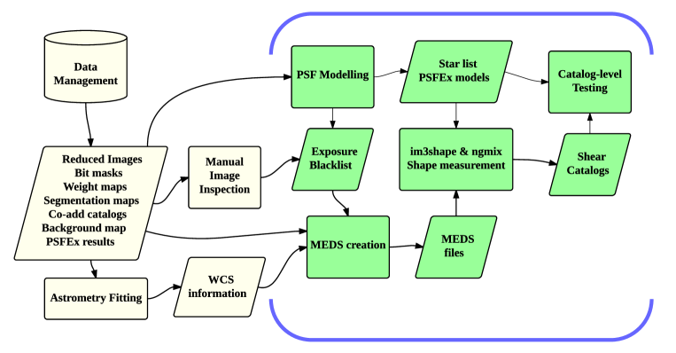
In this paper we present the shear catalogue for the DES Science Verification (SV) data, described in §2. We derive requirements for our systematic uncertainties in §3. The PSF model is described and tested in §4. To facilitate multi-epoch shear measurements, we developed Multi-Epoch Data Structures (MEDS), which we describe in §5. Two sets of simulations that we used for calibration and testing are presented in §6. We present our two shear estimation codes, im3shape and ngmix in §7. Then we submit our catalogues to a suite of null tests, described in §8, which constitutes the main results of this paper. Finally, we describe our final shear catalogues in §9 and conclude in §10. Appendices provide more information on the data structures and catalogue flags. A flowchart outlining the main stages in the production of the shear catalogues is shown in Figure 1.

Figure 1: A flowchart showing the main stages in the production of the shear catalogues. The items inside the blue bracket are done by the weak lensing group in DES and are the principal subject of this paper.

2 Data

The Dark Energy Camera (DECam; Flaugher et al., 2015; Diehl, 2012; Honscheid et al., 2012) was installed on the 4m Victor M. Blanco Telescope at the Cerro Tololo Inter-American Observatory (CTIO) in Chile from June, 2011, to September, 2012 (Diehl et al., 2014). The first light ceremony was September 12, 2012.

DECam holds sixty-two $2048\times 4096$ science CCDs, four $2048\times 2048$ guider CCDs, and eight $2048\times 2048$ focus and alignment CCDs, for a total of 570 megapixels covering a roughly hexagonal footprint. The CCDs were fabricated at Teledyne Dalsa, further processed by Lawrence Berkeley National Laboratory (LBNL), and assembled and tested at Fermilab. Each CCD is 250 microns thick and fully depleted, with two amplifiers per CCD.

The DECam field of view has a diameter of 2.2 degrees on the sky. Unfortunately, one the 62 science CCDs was damaged during commissioning, so we have only 61 working CCDs. The total usable footprint of an exposure, excluding the gaps between the CCDs, totals 2.7 square degrees. Five filters are used during normal survey operations, $g$, $r$, $i$, $z$, $Y$, exchanged using an automated shutter-filter system (Tarlé et al., 2010).

The Dark Energy Survey (DES) officially started taking survey data in August, 2013 (Diehl et al., 2014). It will cover about 5000 square degrees in the South Galactic Cap region, with $\sim$10 visits per field in the $g$, $r$, $i$ and $z$ bands (two visits per year), for a $10\sigma$ limiting magnitude of about 24.1 in the $i$ band. In addition to the main survey, the DES supernova survey contains smaller patches optimized for time-domain science, which are visited more often, and which are useful as a deeper dataset observed with the same instrument.

Before the start of the main survey, a small Science Verification (SV) survey was conducted from November 2012 to February 2013. The strategy was to observe the SV area at 10 different epochs, mimicking the number of visits and total image depth planned for the full 5-year DES survey. The dither pattern matches that of the main survey, which uses large dithers to minimize the impact of any systematic errors related to the location on the field of view. Each tiling is typically observed on different nights to vary the observing conditions as much as possible. Significant depth variations exist in the SV data due to weather, issues with the telescope, and no data quality checks to ensure uniformity (cf. Leistedt et al., 2015).

For the current study we restricted our measurements to the largest portion of the SV area, known as SPT-East (SPT-E for short), an area of approximately 139 square degrees contained within the eastern part of the region observed by the South Pole Telescope (SPT; Carlstrom et al., 2011).

The SV data were reduced by the DES Data Management (DESDM) system (Mohr et al., 2012; Desai et al., 2012), resulting in calibrated and background-subtracted images. Catalogues were produced using the software package Source Extractor (SExtractor; Bertin & Arnouts, 1996; Bertin, 2011). The point spread function was characterized using the PSFEx package (Bertin, 2011; for more details, see §4).

On a set of pre-defined areas of sky, all overlapping single-epoch images were registered and combined into a coadd image using the SCamp and SWarp packages (Bertin et al., 2002; Bertin, 2006).

For weak lensing we used these coadd images only for object detection, deblending, fluxes (for use in photometric redshift measurements, see Sánchez et al., 2014; Bonnett et al., 2015), and for the detailed informational flags which were important for determining a good set of galaxies to use for shear measurement.

In contrast to previous work on DES data by Melchior et al. (2015), we performed object shape measurement directly on all available single-epoch images in which an object was observed, using multi-epoch fitting techniques. See §5 for more details of how we repackaged the data for multi-epoch fitting and §7.1 for a description of the multi-epoch measurement process.

2.1 Object Catalogue

The starting point for our object catalogue was the “SVA1 Gold Catalogue” , which excludes regions of the data that were found to be problematic in some way, due to imaging artefacts, scattered light, failed observations, etc. The selection criteria for the Gold Catalogue included the following:

• Required object to have been observed at least once in each of the $g,r,i,$ and $z$ bands.

• Required Declination to be north of $61^{\circ}S$ to avoid the Large Magellanic Cloud and R Doradus, where the photometric calibration was found to have severe problems.

• Removed regions with a high density of objects with “crazy colours”, i.e. those with any of the following: $g-r<-1,~{}g-r>4,~{}i-z<-1,$ or $i-z>4$. Such regions are usually due to satellite trails, ghosts, scattered light, etc.

• Removed regions with a density less than $3\sigma$ below the mean density.

• Removed regions near bright stars. We eliminated a circular region around all stars detected in the 2-micron All Sky Survey (2MASS; Skrutskie et al., 2006) brighter than $J_{M}=12$ with a mask radius of $r=(-10J_{M}+150)$ arcseconds up to a maximum radius of 120 arcseconds.

• Removed regions with a concentration of objects with large centroid shifts between bandpasses. Some of these objects are just dropout galaxies or large galaxies with complex, wavelength-dependent substructure, but many are due to scattered light, ghosts, satellite trails, etc. 25% of such objects fall into 4% of the total area, so we removed all objects in that 4% on the assumption that the other nearby objects probably have corrupted shapes and photometry.

The full SPT-E area observed during SV totals 163 square degrees. Applying the above selection criteria brings this down to 148 square degrees for the Gold Catalogue.

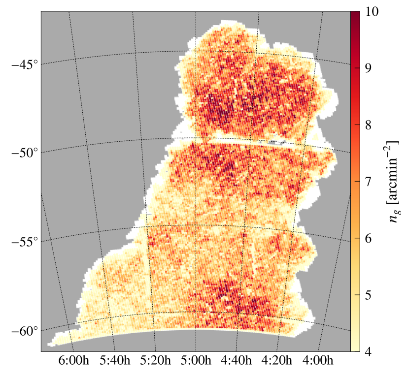
The selection criteria listed above removed galaxies in a non-random way that varied across the sky. We characterized this selection using a geometrical “mask”, implemented as a HEALPIX map (Górski et al., 2005). The HEALPIX map for the DES SPT-E region is shown in Figure 2. The white background represents the Gold Catalogue area. The coloured intensity represents the galaxy number density in the ngmix catalogue (cf. §7.4).

The region used for the weak lensing analysis is somewhat smaller than the full Gold Catalogue region, because we additionally excluded CCD images with poor astrometric solutions (cf. §2.3), poor PSF solutions (cf. §4.2), and blacklisted CCDs containing bright stars, ghosts, airplanes etc. (cf. §5.1). The astrometric cuts in particular removed regions near the edge, since the solutions were poorly constrained there, resulting in a final area for the shear catalogues of 139 square degrees. The intensity map for the im3shape  catalogue (cf. §7.3) looks qualitatively similar, although it is about 40% shallower (cf. §9.3).

Figure 2: A HEALPIX map of the SPT-E region. The white background shows the full “Gold” area. The colours show the galaxy density in the ngmix shear catalogue. (The map for im3shape is qualitatively similar, although about 40% shallower.) The map has HEALPIX resolution nside = 512.

2.2 Galaxy Selection

The preliminary galaxy selection was performed using standard SExtractor outputs from the $i$-band detections in the Gold Catalogue. The selection, in pseudo-code, was

  bright_test = CLASS_STAR > 0.3
                AND MAG_AUTO < 18.0
  locus_test = SPREAD_MODEL +
               3*SPREADERR_MODEL < 0.003
  faint_psf_test = MAG_PSF > 30.0
                   AND MAG_AUTO < 21.0

  galaxies = NOT bright_test
             AND NOT locus_test
             AND NOT faint_psf_test

Within DES, this is called the “Modest Classification” scheme. Bright stars were identified by the standard SExtractor classifier (bright_test). Fainter objects were considered stars if they were near the stellar locus in the SPREAD_MODEL measure, introduced by Desai et al. (2012), which uses a model of the local PSF to quantify the difference between PSF-like objects and resolved objects (locus_test; see also Bouy et al., 2013).

Objects whose best estimate of the total magnitude is much brighter than their PSF magnitude (faint_psf_test) are often spurious detections and were considered “junk” in this classification. Our initial galaxy selection then included every object not classified as either a star or junk by this scheme.

Many faint stars and spurious detections remained in the catalog at this stage. Later, further selection criteria, described in §9.1, were applied based on measurements from the shear pipelines. The initial selection was not intended to produce an accurate galaxy catalogue, but rather to produce a superset of the objects that would eventually be trimmed based on more stringent selection criteria. All objects in this preliminary galaxy catalogue were processed by both shear measurement algorithms (cf. §7).

2.3 Astrometry

For each CCD image we must establish an astrometric solution, i.e. a map from pixel coordinates $(x,y$) to celestial coordinates $(\theta,\phi)$, known as the World Coordinate System (WCS). Since the determination of galaxy shapes is done by a simultaneous fit to the pixel data for all single-epoch exposures covering the galaxy, any misregistration of the exposures will introduce spurious shear signals into the inferred galaxy shapes and sizes.

We found that the astrometric solutions provided by DESDM were not sufficiently accurate for our needs. They included misregistrations of more than 150 milliarcseconds on some CCDs, which induced unacceptably high systematic errors in the galaxy shapes. Here we describe the process we used to improve these solutions to the WCS.

Astrometric solutions for the SV exposures were assumed to take the form

$$P(\theta,\phi)=E\left(C(x,y)\right),$$ (2.1)

where $P$ is a gnomonic projection from the (curved) sky on to a planar coordinate system, using a chosen field coordinate for the pole of the projection; $E$ is an affine transformation chosen to be distinct for each CCD image of each exposure; and $C$ is a cubic polynomial mapping that is common to all exposures in a given filter with a given CCD. In the nomenclature of the SCamp code, $C$ is the “instrument” solution, and $E$ is the “exposure” solution.

The instrument solution $C$ was derived as follows. We took a series of $\approx 20$ exposures of a rich star field in succession, with the telescope displaced by angles ranging from 10 arcseconds up to the field of view of the camera. Coordinates of stars were determined in the pixel coordinates of each exposure, and we adjusted the parameters of the map in equation 2.1 to minimize the internal disagreement between sky coordinates of all the observations of each star. The solution also minimized the discrepancies between the positions of stars in the 2MASS (Skrutskie et al., 2006) catalogue and our measurements of these stars, thereby anchoring the absolute pointing and scale of our astrometric maps.

All 20 coefficients of the cubic polynomial $C$ were left free for each of the 61 functional CCDs (cf. Diehl et al., 2014; Flaugher et al., 2015). While fitting the star field data, we forced all CCDs in a given exposure to share a common affine map $E$, so there were 6 additional free parameters in the fit for each exposure. The instrument maps $C$ derived in this way were assumed to apply to all SV exposures taken with the same CCD in the same filter. The process was repeated for each of the $g$, $r$, $i$, $z$, $Y$ filters.

Repeating the above “star flat” procedure every few months revealed small changes in the astrometric map, consistent with rigid motion of some CCDs relative to the others at a level of $\approx 10$ milliarcseconds, probably occurring when the camera was cycled to room temperature for occasional engineering tasks.

To account for these small shifts, we determined an independent $E$ function (6 degrees of freedom) for each CCD image in the SV data in another round of fitting. In this second stage we minimized the disagreements between positions reported for all CCDs that contribute to each DES coadd image. The coefficients of the affine transformations $E$ were allowed to float, but the higher-order polynomials $C$ were held fixed at the values determined from the star field data. These solutions again minimized residuals with respect to matching sources from the 2MASS catalogue in order to fix the absolute position on the sky.

Note that the principal effects of differential chromatic refraction (DCR) are a shift and a shear along the direction toward zenith, which are both properly included as part of the affine transformation $E$ for each CCD. We did not, however, make any attempt to address the intra-band chromatic effects related to DCR (cf. Plazas & Bernstein, 2012; Meyers & Burchat, 2015).

The RMS disagreement between sky positions of bright stars inferred from distinct DES exposures are consistent with errors in the astrometric maps of 10–20 milliarcseconds RMS in each coordinate. We found these errors to be coherent over arcminute scales in a given exposure, but were uncorrelated between distinct exposures. We interpret this to mean the remaining relative astrometric errors are dominated by stochastic atmospheric distortions (cf. Heymans et al., 2012a). Indeed, equation 8 of Bouy et al. (2013) predicts an RMS astrometric residual due to the atmosphere of order 10 milliarcseconds for our field of view and exposure time.

We found some remaining astrometric errors that were coherent over time and correlated with position on the detector array, which are consistent with small components of the electric fields transverse to the surface of the CCD in some places (Plazas et al., 2014). These residuals are at the few milliarcsecond level, which is small enough to be irrelevant for SV data reductions.

3 Requirements on Systematic Errors

In this section, we derive the requirements for systematic uncertainties on the shear estimates for the DES SV data. These requirements will be used to assess the quality of the PSF and shear catalogues in subsequent sections.

Throughout this paper we will use the notation $e=e_{1}+ie_{2}=|e|\exp(2i\phi)$ as the complex-valued shape of each galaxy. We define the shape $e$ such that the expectation value of the mean shape for an ensemble of galaxies is an estimate of the mean reduced gravitational shear acting on those galaxies

$$\langle e\rangle=g\equiv\frac{\gamma}{1-\kappa},$$ (3.1)

where $\gamma$ and $\kappa$ are the shear and convergence, respectively (see e.g. Hoekstra, 2013 for a review of weak lensing concepts and terminology).

For a galaxy with elliptical isophotes, one finds that $|e|=(a-b)/(a+b)$ satisfies equation 3.1, where $a$ and $b$ are the semi-major and semi-minor axes of the ellipse. However, galaxies do not in general have elliptical isophotes, so this definition is of little practical value. For the more general case, the estimator

$$e=\frac{I_{xx}-I_{yy}+2iI_{xy}}{I_{xx}+I_{yy}+2\sqrt{I_{xx}I_{yy}-I_{xy}^{2}}}$$ (3.2)

has been proposed by Seitz & Schneider (1997), where the second moments of the intensity profile $I(x,y)$ are defined as

$$I_{\mu\nu}=\frac{\int dxdyI(x,y)(\mu-\bar{\mu})(\nu-\bar{\nu})}{\int dxdyI(x,y)}.$$ (3.3)

But since neither shear algorithm in this paper uses equation 3.2 directly, we consider equation 3.1 to be the functional definition of what we mean by the shape of an arbitrary galaxy. See §7.3.1 and §7.4.1 for details about the im3shape and ngmix estimators of $e$.

While equation 3.1 is our goal for the shape estimates in our catalogue, it is inevitable that there will be systematic errors in the shape measurements. A convenient parameterization, based on one first proposed by Heymans et al. (2006), uses a first-order expansion of the form,

$$\langle e\rangle=(1+m)g_{\mathrm{true}}+\alpha e_{\textsc{psf}}+c,$$ (3.4)

where $g_{\mathrm{true}}$ denotes the value that would be obtained from an ideal error-free shape estimator, $m$ quantifies the multiplicative error, $\alpha$ measures the leakage of the PSF shape into the galaxy shapes, and $c$ represents other sources of additive error.

Note that $m$ can in principle be different for each of the two components $e_{1}$ and $e_{2}$. However, we find in practice that the two coefficients are generally very close to equal when they can be measured separately, so we simply take $m$ to be a single real value here. Similarly, $\alpha$ could in principle have up to 4 components if the leakage were anisotropic and involved cross terms, but we do not see evidence for anything beyond a real-valued $\alpha$ in practice.

The leakage term $\alpha e_{\textsc{psf}}$ is commonly (e.g. Heymans et al., 2006) implicitly folded into the general additive error term, $c$, but we have found it useful to retain it explicitly, since PSF leakage can be one of the more difficult additive errors to correct. Furthermore, Mandelbaum et al. (2015) found that the additive systematic errors for essentially all of the methods submitted to the GREAT3 challenge were well-described by $\alpha e_{\textsc{psf}}$, which motivates us to include it as an explicit term in equation 3.4.

3.1 Shear Correlation Functions

We set our requirements on the various kinds of systematic errors according to how they propagate into the shear two-point correlation functions (defined as in Jarvis et al., 2003):

$$\xi_{+}(\theta) =\left\langle e^{*}(\mathbf{x})e(\mathbf{x}+\boldsymbol{\theta})\right\rangle$$ (3.5)

$$\xi_{-}(\theta) =\left\langle e(\mathbf{x})e(\mathbf{x}+\boldsymbol{\theta})\exp(-4i\arg(\boldsymbol{\theta}))\right\rangle,$$ (3.6)

where ^∗ indicates complex conjugation.

Substituting equation 3.4 into these equations and assuming the three types of systematic errors are uncorrelated (which is not necessarily true in general, but is a reasonable assumption for setting requirements), we find

$$\delta\xi_{i}(\theta)\simeq 2m\xi_{i}(\theta)+\alpha^{2}\xi_{i}^{pp}(\theta)+\xi_{i}^{cc}(\theta)$$ (3.7)

to leading order in each type of systematic, where $i\!\in\!\{+,-\}$, $\delta\xi_{i}$ are the systematic errors in the two correlation functions, $\xi_{i}^{pp}$ are the auto-correlation functions of the PSF shapes, and $\xi_{i}^{cc}$ are the auto-correlation functions of the additive error, $c$.

To set requirements on $\delta\xi_{i}$, we consider how the errors will affect our estimate of the cosmological parameter $\sigma_{8}$, the present day amplitude of the (linear) matter power spectrum on the scale of $8h^{-1}$ Mpc. Our requirement is that the systematic errors change the estimated value of $\sigma_{8}$ by less than 3%, $\delta\sigma_{8}/\sigma_{8}<0.03$. This value was chosen to be about half of the expected statistical uncertainty on $\sigma_{8}$ for the DES SV survey.

Propagating this limit to the shear correlation functions, we obtain the requirement

$$\delta\xi^{\mathrm{max}}_{i}=\frac{\partial\xi_{i}}{\partial\sigma_{8}}\delta\sigma_{8}.$$ (3.8)

This constraint assumes that errors are fully correlated across $\theta$; assuming independent errors would be less restrictive.

Figure 3: Requirement for the maximum systematic error contribution to the shear correlation functions. The blue lines correspond to $\delta\sigma_{8}/\sigma_{8}=0.03$ for each of the correlation functions $\xi_{+}$ (solid) and $\xi_{-}$ (dashed). The top and bottom panels shows the requirement for the absolute and relative error in the correlation functions.

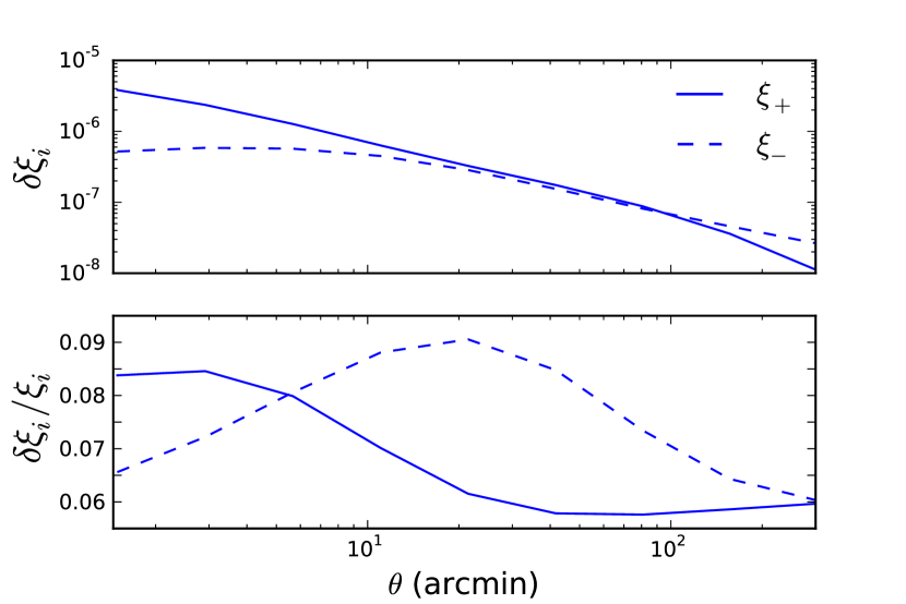
Figure 3 shows the resulting requirements for $\delta{\xi_{i}}$ derived for a flat $\Lambda$CDM central cosmological model with $\sigma_{8}=0.82$, $\Omega_{b}=0.047$ and $\Omega_{c}=0.2344$, $h=0.7$ and $n_{s}=0.96$.

We will apply this requirement to a number of different potential sources of systematic error. If each of them just barely pass the requirement, this would be a problem, since the total net systematic error would then exceed the requirement. We attempt to quantify the total realized systematic error in the shear measurements in §8.7; it is this total error that must be propagated into the next stage(s) of the analysis, along with any other non-measurement sources of systematic error (e.g. photometric redshift errors and intrinsic alignments) that may be relevant for each specific science application.

3.2 Multiplicative and Additive Errors

From equation 3.7, we find that the requirement on the multiplicative bias, $m$, is

$$|m|<\frac{1}{2}\left|\frac{\delta\xi^{\mathrm{max}}_{i}}{\xi_{i}}\right|.$$ (3.9)

As can be seen from the lower panel in Figure 3, the most stringent requirement on $\delta\xi_{i}/\xi_{i}$ is about 0.06, yielding a requirement on the multiplicative error of

$$|m|<0.03.$$ (3.10)

The requirement on the additive systematic error is somewhat more complicated, since it is the correlation function of the additive systematic that matters. For a systematic error that is coherent over small spatial scales (less than $\sim 1$ arcminute), the requirement comes from the zero-lag value of $\delta\xi_{+}$ in Figure 3, $\langle c^{2}\rangle<\delta\xi^{\mathrm{max}}_{+}(0)$, or

$$c_{\mathrm{rms}}<2\times 10^{-3}.$$ (3.11)

For additive errors that have longer correlation lengths, we will need to be more careful about calculating the correlation function of the systematic error. The requirement in this case is

$$|\xi_{i}^{cc}(\theta)|<\delta\xi^{\mathrm{max}}_{i}(\theta)$$ (3.12)

using the function shown in Figure 3. The most notable example of this will be systematic effects due to the PSF: both leakage and modeling errors, which will be discussed in the next two sections.

Note that we do not need to satisfy these requirements for all values of $\theta$. The statistical uncertainties on $\xi_{+,-}(\theta)$ become much larger at large scales, so such scales are not as important for constraining cosmology as smaller scales. In practice, equation 3.12 should ideally be satisfied for scales $\theta<100$ arcminutes, where $\xi_{+,-}(\theta)$ are relatively well-measured.

We note that these results are broadly consistent with those of Amara & Réfrégier (2008), who derived requirements for a tomographic weak lensing survey, performing joint constraints on the set of cosmological parameters for a $w$CDM model. They found requirements of $|m|<4.0\times 10^{-2}$ and $c_{\mathrm{rms}}<2.1\times 10^{-3}$ for DES SV survey parameters, which are in rough agreement with the requirements quoted above.

3.3 PSF Leakage

The requirements for the PSF leakage term in equation 3.4 can be obtained from the general requirement on additive errors, equation 3.12.

$$\alpha^{2}\xi_{i}^{pp}(\theta)<\delta\xi^{\mathrm{max}}_{i}(\theta),$$ (3.13)

which can be solved for $\alpha$ as

$$|\alpha|<\left(\frac{\delta\xi^{\mathrm{max}}_{i}(\theta)}{\xi_{i}^{pp}(\theta)}\right)^{\frac{1}{2}}.$$ (3.14)

Figure 4: Requirement for the PSF leakage factor $\alpha$ based on the relative error in $\sigma_{8}$ being less than 3%.

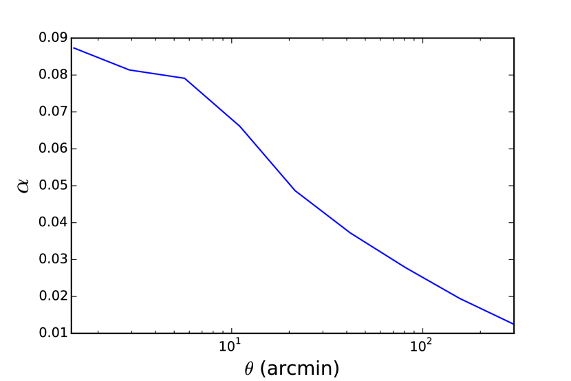
Figure 4 shows this requirement on $\alpha$ as a function of $\theta$ using the observed $\xi_{+}^{pp}$ for DES SV data. The requirement arising from $\xi_{-}^{pp}$ is always larger than 0.05 and is not shown.

In general, the amount of leakage of PSF shapes into galaxy shapes from an imperfect correction scheme is not expected to vary with scale. Rather, we can use Figure 4 to determine a conservative requirement for $\alpha$ that would be applicable for scales $\theta<100$ arcminutes:

$$|\alpha|<0.03.$$ (3.15)

We will estimate $\alpha$ from the data in §8.2.

3.4 PSF Model Errors

We now consider errors in the modeling of the PSF itself. The previous section dealt with the possibility of the galaxy shear estimation algorithm imperfectly accounting for the PSF convolution and letting some of the PSF shape leak into the galaxy shape. However, even a perfect PSF correction scheme can suffer systematic biases if the PSF model itself is biased.

As our starting point, we use the unweighted moments approximation of Paulin-Henriksson et al. (2008), who give the bias on the measured galaxy ellipticity in terms of errors in the PSF model (their equation 13):

$$\delta e_{\mathrm{sys}}=\left(e-e_{\textsc{psf}}\right)\left(\frac{T_{\textsc{psf}}}{T_{\mathrm{gal}}}\right)\frac{\delta T_{\textsc{psf}}}{T_{\textsc{psf}}}-\left(\frac{T_{\textsc{psf}}}{T_{\mathrm{gal}}}\right)\delta e_{\textsc{psf}},$$ (3.16)

where $T\!\equiv\!I_{xx}\!+\!I_{yy}$ is the intensity-weighted second moment of the radius (written as $R^{2}$ in their paper). $T_{\mathrm{gal}}$ refers to the intrinsic galaxy size, unconvolved by the PSF.

Constructing the shear correlation function with this model, we find that the systematic error in $\xi_{+}$ is

$$\delta\xi_{+}(\theta) =2\left\langle\frac{T_{\textsc{psf}}}{T_{\mathrm{gal}}}\frac{\delta T_{\textsc{psf}}}{T_{\textsc{psf}}}\right\rangle\xi_{+}(\theta)+\left\langle\frac{T_{\textsc{psf}}}{T_{\mathrm{gal}}}\right\rangle^{2}\rho_{1}(\theta)$$

$$\quad-\alpha\left\langle\frac{T_{\textsc{psf}}}{T_{\mathrm{gal}}}\right\rangle\rho_{2}(\theta)+\left\langle\frac{T_{\textsc{psf}}}{T_{\mathrm{gal}}}\right\rangle^{2}\rho_{3}(\theta)$$

$$\quad+\left\langle\frac{T_{\textsc{psf}}}{T_{\mathrm{gal}}}\right\rangle^{2}\rho_{4}(\theta)-\alpha\left\langle\frac{T_{\textsc{psf}}}{T_{\mathrm{gal}}}\right\rangle\rho_{5}(\theta),$$ (3.17)

where $\rho_{1}(\theta)$ and $\rho_{2}(\theta)$ are defined as (cf. Rowe, 2010)

$$\rho_{1}(\theta) \equiv\left\langle\delta e_{\textsc{psf}}^{*}(\mathbf{x})\delta e_{\textsc{psf}}(\mathbf{x}+\boldsymbol{\theta})\right\rangle$$ (3.18)

$$\rho_{2}(\theta) \equiv\left\langle e_{\textsc{psf}}^{*}(\mathbf{x})\delta e_{\textsc{psf}}(\mathbf{x}+\boldsymbol{\theta})\right\rangle,$$ (3.19)

and we introduce three new statistics defined as

$$\rho_{3}(\theta) \equiv\left\langle\left(e_{\textsc{psf}}^{*}\frac{\delta T_{\textsc{psf}}}{T_{\textsc{psf}}}\right)\!(\mathbf{x})\left(e_{\textsc{psf}}\frac{\delta T_{\textsc{psf}}}{T_{\textsc{psf}}}\right)\!(\mathbf{x}+\boldsymbol{\theta})\right\rangle$$ (3.20)

$$\rho_{4}(\theta) \equiv\left\langle\delta e_{\textsc{psf}}^{*}(\mathbf{x})\left(e_{\textsc{psf}}\frac{\delta T_{\textsc{psf}}}{T_{\textsc{psf}}}\right)\!(\mathbf{x}+\boldsymbol{\theta})\right\rangle$$ (3.21)

$$\rho_{5}(\theta) \equiv\left\langle e_{\textsc{psf}}^{*}(\mathbf{x})\left(e_{\textsc{psf}}\frac{\delta T_{\textsc{psf}}}{T_{\textsc{psf}}}\right)\!(\mathbf{x}+\boldsymbol{\theta})\right\rangle.$$ (3.22)

There are corresponding terms for $\delta\xi_{-}$, which are negligible in practice and thus uninteresting as requirements.

The first term in equation 3.17 is a multiplicative systematic, so the relevant requirement comes from equation 3.10. We approximate the ensemble average as a product of two averages to set a requirement on the mean error in the PSF size

$$\left|\left\langle\frac{\delta T_{\textsc{psf}}}{T_{\textsc{psf}}}\right\rangle\right|<0.03\left\langle\frac{T_{\textsc{psf}}}{T_{\mathrm{gal}}}\right\rangle^{-1}.$$ (3.23)

This represents an error due to improperly accounting for the “dilution”, the amount by which the blurring of the PSF makes objects rounder than they originally were. Estimating the wrong PSF size will lead to a systematic multiplicative bias in the inferred galaxy shapes.

The other terms are additive errors, contributing to $\xi_{+}^{cc}(\theta)$, so the requirements from equation 3.12 are that each term be less than $\delta\xi^{\mathrm{max}}_{+}(\theta)$:

$$|\rho_{1,3,4}(\theta)| <\left\langle\frac{T_{\textsc{psf}}}{T_{\mathrm{gal}}}\right\rangle^{-2}\delta\xi^{\mathrm{max}}_{+}(\theta)$$ (3.24)

$$|\rho_{2,5}(\theta)| <|\alpha|^{-1}\left\langle\frac{T_{\textsc{psf}}}{T_{\mathrm{gal}}}\right\rangle^{-1}\delta\xi^{\mathrm{max}}_{+}(\theta).$$ (3.25)

We will test these requirements for our PSF model below in §4.4.

For our data, we compute the factor $\langle T_{\textsc{psf}}/T_{\mathrm{gal}}\rangle$ that appears in these requirements to be 1.20 for im3shape and 2.42 for ngmix; the latter is larger because the final galaxy selection for the ngmix catalogue keeps more small galaxies than the im3shape selection. We use the ngmix value in §4.4, as it gives the more stringent requirement. For $\alpha$, we conservatively use the value 0.03. We will find in §8.2.2 that both codes estimate $\alpha$ to be consistent with zero; however, it is not estimated much more precisely than this value.

4 PSF Estimation

The principal confounding factor that must be addressed in order to measure accurate shears is the convolution of the galaxy surface brightness profiles by the point-spread function (PSF). The net PSF is due to quite a number of physical processes including atmospheric turbulence, telescope and camera aberrations, guiding errors, vibrations of the telescope structure, and charge diffusion in the CCDs, among other more subtle effects. Furthermore, this PSF is not constant, but varies both spatially over the focal plane and temporally from one exposure to the next. The atmospheric component varies approximately according to a Kolmogorov turbulent spectrum. The optical aberrations have characteristic patterns due to features in the telescope optics.

Fortunately, we do not need to have a complete physical model of all the contributors to the PSF in order to accurately characterize it. Instead, we build an empirical model, based on observations of stars, which we interpolate to obtain an estimate of the PSF at any location on the focal plane. In this section, we describe how we select appropriate stars to use, and then build and test the PSF model.

4.1 Initial Identification of Stars

We first selected the stars to be used to constrain the PSF model. As stars are point sources, observations of them provide a sample image of the PSF at the location of each star. We desired a high-purity sample of fairly bright stars to make sure we did not erroneously consider images of small, faint galaxies to be images of the PSF, as that would bias the resulting PSF model.

We found that, for some CCD images, the sets of objects identified as stars by the Modest Classification scheme included a relatively high number of galaxies, and in other cases too few stars were identified. The cause of these failures is dependent on many factors, but may be partly related to the use of coadd data for the classification. The coadd PSF can change abruptly at the locations of chip edges in the original single-epoch images, which may have affected the stellar classification near these discontinuities.

Ultimately, the problems with the modest classifier were common enough that we decided to develop a new algorithm tailored specifically to the identification of a pure set of PSF stars. Our algorithm works on each CCD image separately, using a size-magnitude diagram of all the objects detected on the image. For the magnitude, we use the SExtractor measurement MAG_AUTO. For the size, we use the scale size, $\sigma$, of the best-fitting elliptical Gaussian profile using an adaptive moments algorithm. We found that these measures produce a flatter and tighter stellar locus than the FLUX_RADIUS value output by SExtractor, and is thus better suited for selection of stars. As a further improvement, we initialize the algorithm with some stars identified by SExtractor to have CLASS_STAR between 0.9 and 1.0. This was found to give a decent estimate of the size of the PSF, providing a good starting guess for the location of the stellar locus.

Figure 5: An example size-magnitude diagram for a single CCD image, used to identify stars. The size $T=2\sigma^{2}$ is based on the scale size of the best-fitting elliptical Gaussian. The pink and green points are the objects initially identified as stars. The green points are the ones that pass our selection criteria outlined in §4.2, most notably the magnitude cut to avoid objects contaminated by the brighter-fatter effect. These objects are then used to constrain the PSF model. The blue circles show an an alternate star classification, called the Modest Classification within DES, which was found not to work as well for our specific purpose.

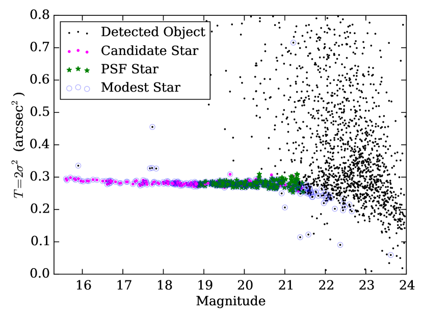
The stars are easily identified at bright magnitudes as a locus of points with constant size nearly independent of magnitude. The galaxies have a range of sizes, all larger than the PSF size. Thus, the algorithm starts with a tight locus at small size for the stars and a broad locus of larger sizes for the galaxies for objects in the brightest 5 magnitudes (excluding saturated objects). Then the algorithm proceeds to fainter magnitudes, building up both loci, until the stellar locus and the galaxy locus start to merge. The precise magnitude at which this happens is a function of the seeing as well as the density of stars and galaxies in the particular part of the sky being observed. As such the faint-end magnitude of the resulting stellar sample varies among the different exposures.

Figure 5 shows such a size-magnitude diagram for a representative CCD image. The stellar locus is easily identified by eye, and the stellar sample identified by our algorithm is marked in pink and green. The pink points are stars that are removed by subsequent steps in the process outlined below, while the green points are the stars that survive these cuts. The blue circles show the objects identified as stars according to the Modest Classification, which includes more outliers and misses some of the objects clearly within the stellar locus.

While the algorithm we currently use is found to work well enough for the SV data, we plan to investigate whether the neural net star-galaxy separator recently developed by Soumagnac et al. (2015) is more robust or could let us include additional stars.

4.2 Selection of PSF Stars

Some of the stars in this sample are not appropriate to use for PSF modeling, even ignoring the inevitable few galaxies that get misidentified as stars. The CCDs on the Dark Energy Camera each have six spots where 100 micron thick spacers were placed behind the CCDs when they were glued to their carriers (cf. Flaugher et al., 2015), which affects the electric field lines near each 2mm $\times$ 2mm spacer. These features, which we call tape bumps, distort the shapes in those parts of the CCDs, so the stellar images there are not accurate samples of the PSF. We exclude any star whose position is within 2 PSF FWHM separation of the outline of a tape bump. The tape bumps are relatively small, so this procedure excludes less than 0.1% of the total area of the CCD, but removes a noticeable bias in the PSF model near the bumps.

Another problem we addressed with regards to star selection is the so-called “brighter-fatter effect” (Antilogus et al., 2014; Guyonnet et al., 2015). As charge builds up in each pixel during the exposure, the resulting lateral electric fields and increased lateral diffusion push newly incoming charges slightly away from the existing charge. This makes bright objects appear a bit larger than fainter objects. In addition, an asymmetry in the magnitude of the effect between rows and columns can make bright stars more elliptical. The galaxies we used for weak lensing are generally faint, so the brightest stars do not accurately sample the PSF that we need to measure. Furthermore, the brighter-fatter effect does not manifest as a convolution of the signal, so the bright stars do not even provide an estimate of the correct PSF to be used for bright galaxies.

Figure 6: The residual size (top) and shape (bottom) of stars relative to that of the PSF model as a function of magnitude. The hatched region on the left shows the magnitude range of the stars we exclude from the sample to reduce the impact of the brighter-fatter effect.

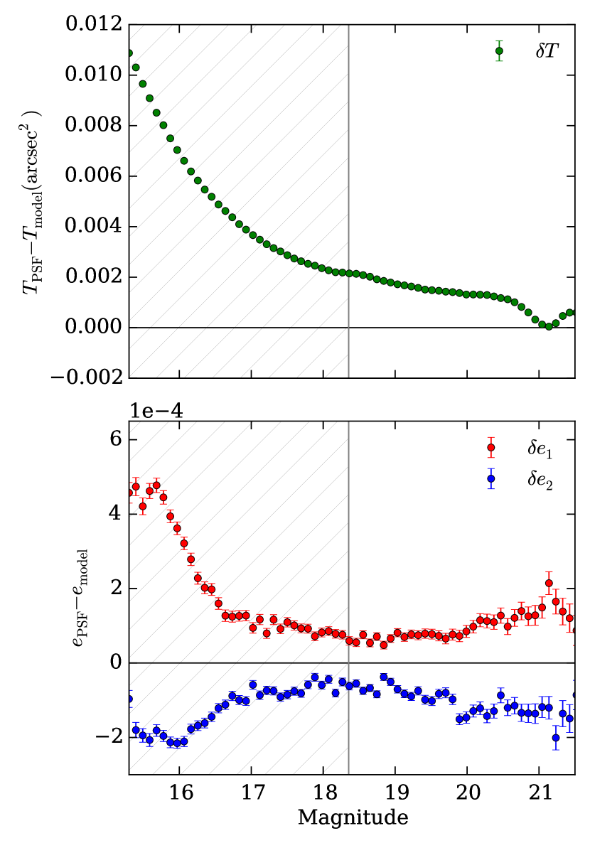
The appropriate solution is to move the shifted charge back to where it would have fallen in the absence of this effect. This will be implemented in future DES data releases (Gruen et al., 2015). For the current round of catalogues, we instead partially avoided the problem by removing the brightest stars from our sample. Specifically, we removed all stars within 3 magnitudes of the saturation limit for the exposure. That is, in our final selection of PSF stars we required that the brightest pixel in the stellar image be less than 6% of the pixel full well. Since the brighter-fatter effect scales approximately linearly with flux, this reduces the magnitude of the effect by a factor of 16. We were left with stars of lower $S/N$, so it is not the ideal solution, but it is an acceptable interim measure (as we demonstrate below) until the more sophisticated solution can be implemented.

In Figure 6 we show the mean difference between the measured sizes of observed stars and the size of the PSF model at their locations, using the model described below in §4.3. For the measurements of the sizes and shapes described here, we used the implementation of the HSM (Hirata & Seljak, 2003; Mandelbaum et al., 2005) algorithm included in the GalSim software package. The hatched region marks the range we excluded to avoid the spurious increase in PSF size from the brighter-fatter effect. In Figure 6 we have also shown the mean difference in ellipticity due to the brighter-fatter effect; it affects the shapes of the stars as well as the size.

We do not yet understand why the residual sizes and shapes shown in Figure 6 do not level off to zero at fainter magnitudes where the brighter-fatter effect is negligible. The requirement on this residual value is given by equation 3.23. We calculate $\langle\delta T_{\textsc{psf}}/T_{\textsc{psf}}\rangle$ to be $0.0044$, which is well below our requirement of 0.013 for the SV data. However, this residual will not be acceptable for future DES analyses, so we will need to investigate what is causing the problem and fix it.

Figure 7: The distribution of the number of stars per CCD image used for constraining the PSF model.

Figure 8: The distribution of the median FWHM of the PSF stars in the non-blacklisted exposures (cf. §5.1). The $r$, $i$ and $z$-band exposures are indicated from top to bottom within each bar in red, purple, and black.

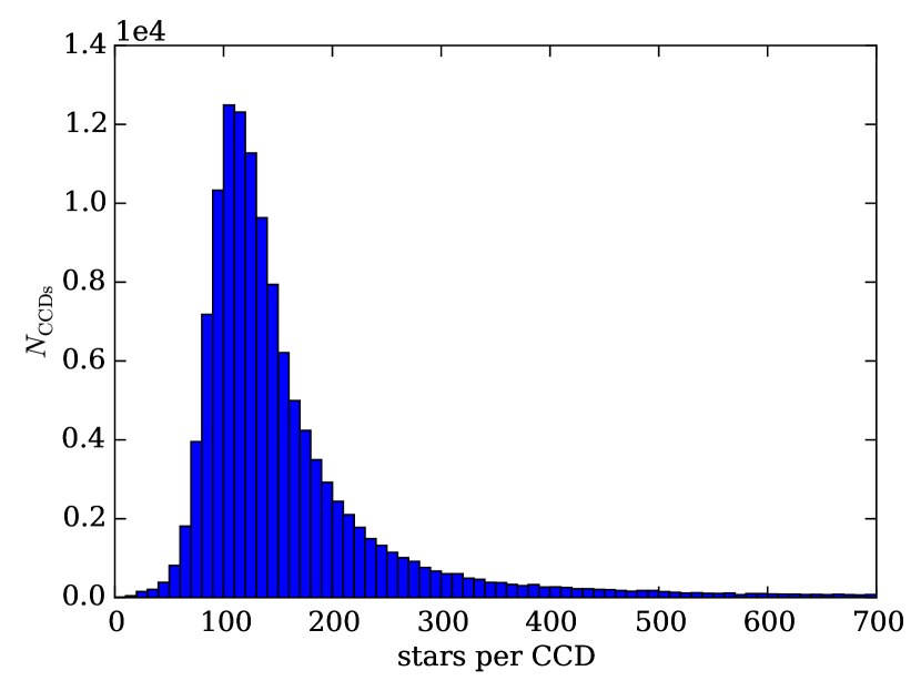
In the complete process described above we find a median of 130 useful stars per CCD image, which we use to constrain the PSF model. The distribution is shown in Figure 7.

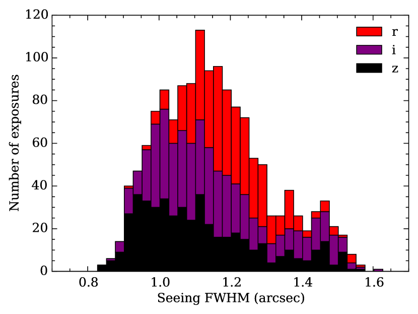
In Figure 8 we show the distribution of the median measured full-width half-max (FWHM) for the PSF stars used in our study, restricted to the exposures used for shear measurements. The overall median seeing of these exposures was 1.08 arcsec. The $r$, $i$ and $z$-bands had median seeing of 1.11, 1.08, and 1.03 arcsec respectively. This was somewhat worse than expected (0.9 arcesec) and reflects the fact that a number of problems related to the instrument, telescope, and control software were being diagnosed and fixed concurrently with the observations. The realized seeing has significantly improved in the subsequent main survey observations (Diehl et al., 2014).

For some CCD images no stars passed our final selection criteria, usually because the initial stellar selection could not find any stars or no stars survived the magnitude cuts. For instance, this can happen when there is a very bright object in the image that essentially masks out the entire image, leaving zero or very few objects detected. In less extreme cases, a bright object can sufficiently contaminate the fluxes and sizes of the other detections that the stellar locus is either difficult to find or merges with the galaxy locus at a fairly bright magnitude, such that the brighter-fatter cut excludes the entire sample.

Whenever the process failed for any reason on a given CCD image, we flagged the image and excluded it from being used in subsequent shear estimation. We also flagged images with less than 20 identified PSF stars, since it is difficult to accurately interpolate the PSF model with so few stars. These flagged images were added to the set of blacklisted images described in §5.1.

4.3 PSF Measurement and Interpolation

Figure 9: Whisker plots of the mean PSF pattern (left) and of the mean residual after subtracting off the model PSF (right) as a function of position in the focal plane. The length of each whisker is proportional to the measured ellipticity, and the orientation is aligned with the direction of the ellipticity. There is still some apparent structure in the plot of the residuals, but the level is below the requirements for SV science. Reference whiskers of 1% and 3% are shown at the bottom of each plot, and we have exaggerated the scale on the right plot by a factor of 10 to make the residual structure more apparent.

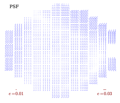
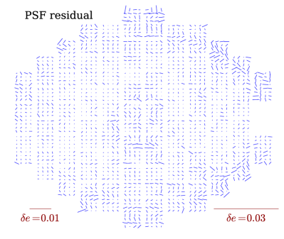
To measure the PSF and its spatial variation on each CCD, we used the software package PSFEx (Bertin, 2011). Normally, PSFEx takes as input the full list of objects detected by SExtractor and finds the bright stars automatically. However, as described in §4.2, we removed some of the stars in the catalogue to avoid the brighter-fatter effect and the tape bumps. This edited catalogue of stars was then passed to PSFEx.

We used the BASIS_TYPE = PIXEL_AUTO option, which uses pixelated images to model the PSF profile, rather than fitting to some functional form. In Kitching et al. (2013), for undersampled PSFs a fixed oversampling was found to perform better than the default PSFEx choice; therefore, we forced the oversampling of these images to be a factor of 2 finer than the original pixel size with PSF_SAMPLING = 0.5. The basis images are set to be $101\times 101$ in the resampled pixels, or approximately 13 arcseconds on a side.

For the interpolation, we used a second order polynomials in chip coordinates, interpolated separately on each CCD. Specifically, we use the following parameters:

PSFVAR_KEYS = XWIN_IMAGE,YWIN_IMAGE
PSFVAR_GROUPS = 1,1
PSFVAR_DEGREES = 2

We found that there was not much gain in using higher order polynomials than this and some evidence that they were overfitting the noise for some CCDs. So we decided to use second order in all cases.

To assess the quality of the PSF interpolation, we first examined the differences between the measured shapes (using the HSM algorithm again) of actual stars on the image and the corresponding values for the PSFEx model at the locations of these stars. In Figure 9 we show the whisker plots of the PSF and the residuals as a function of position on the focal plane. The residual whiskers are small, but not quite zero. The impact of these spatially correlated residuals are investigated below in §4.4, and we will show that they meet the requirements for science with SV data.

We believe the remaining structure seen in the residual plot is largely due to the fact that the PSF modeling and interpolation is done in pixel coordinates rather than sky coordinates. Therefore, the interpolation must also include the effects of the non-uniform WCS. In particular, the distortion due to the telescope optics is a fifth order radial function, but we fit the PSF with only a second order polynomial on each CCD. This is most markedly seen in the CCDs near the edges of the field of view where the residuals look consistent with a fifth order radial function after the local second order approximation has been subtracted off. One of our planned improvements to the analysis is to interpolate the PSF in sky coordinates rather than pixel coordinates, so that WCS variations can be modeled separately from real PSF variations. We expect this change to remove most of the remaining residual PSF pattern.

4.4 PSF Model Diagnostics

Errors in the PSF model, and particularly errors in the interpolation, will directly affect the shear estimates of galaxies, since they would be accounting for the effect of the PSF convolution incorrectly, as discussed in §3.4. If the PSF errors were random, independent values for each galaxy, they would constitute merely an additional contribution to the shear measurement uncertainty, which would be highly subdominant to other sources of statistical noise, such as the unknown intrinsic shapes of the galaxies. However, this is not the case. Because the PSF is interpolated between stars, the errors in the PSF estimate are correlated among nearby galaxies. The two-point correlation function of these errors will directly impact the two-point correlation function of the shear estimates, which means they would be a systematic error, as quantified in equation 3.17.

Rowe (2010) describes two diagnostic functions to quantify the level of interpolation errors in the PSF model using the measured shapes of stars and the interpolated value of the model at the locations of these stars. As we already introduced in §3.4,

$$\rho_{1}(\theta) \equiv\left\langle\delta e_{\textsc{psf}}^{*}(\mathbf{x})\delta e_{\textsc{psf}}(\mathbf{x}+\boldsymbol{\theta})\right\rangle$$ (4.1)

$$\rho_{2}(\theta) \equiv\left\langle e_{\textsc{psf}}^{*}(\mathbf{x})\delta e_{\textsc{psf}}(\mathbf{x}+\boldsymbol{\theta})\right\rangle,$$ (4.2)

where $\delta e_{\textsc{psf}}$ represents the difference between the measured ellipticity of the observed stars and the ellipticity of the PSFEx models at the same locations, which is an estimate of the systematic uncertainty in the shape of the PSF model at those locations.

In addition, we test three other statistics that appear at the same order of the expansion of PSF model errors, involving errors in the PSF size, $T_{\textsc{psf}}$, which we call $\rho_{3}$, $\rho_{4}$, and $\rho_{5}$. They are defined in equations 3.20 – 3.22 and are generally smaller than the two described by Rowe (2010).

Figure 10: The $\rho$ statistics for the PSF shape residuals. Negative values are shown in absolute value as dotted lines. The shaded regions are the requirements for SV data.

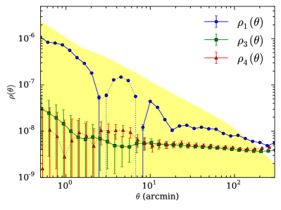
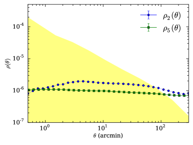
Figure 10 shows the results for these five statistics. The shaded regions show the requirements, from equations 3.24 & 3.25. In all cases, the results are seen to be passing our requirements for scales less than about 100 arcminutes. We see in Figure 10 that $\rho_{1}$ changes sign twice and is below the requirement line by only a factor of $\sim$ 2. However, our requirements make the conservative assumption that additive errors are fully correlated across scales. So we have directly propagated the measured $\rho_{1}$ through to the bias on $\sigma_{8}$ and found the influence on $\sigma_{8}$ to be much less than one percent.

Of course, the PSFEx model describes the full surface brightness profile of the PSF, not just its shape $e_{\textsc{psf}}$ and size $T_{\textsc{psf}}$. However, these are the dominant ways that errors in the PSF model could affect the galaxy shapes, so these statistics are the most important checks of the model accuracy.

5 Multi-Epoch Data Structures

As outlined in §2, we used the coadd images for object detection and deblending. For shear measurement we worked directly with the pixel data from the original single-epoch images (cf. §7.1). To simplify the bookkeeping we developed a new data storage format, which we named Multi-Epoch Data Structures (MEDS).

We created a MEDS file corresponding to each coadd image. In these files we stored a postage stamp for each observation of every object detected in the coadd image along with the corresponding weight maps, segmentation maps, and other relevant data. The postage stamps for each coadd object were stored contiguously in the file, making sequential access of individual objects efficient. The files are quite large, so loading the whole file into memory is not generally feasible, but it is also not necessary.

The postage stamps from the original single-epoch images were sky-subtracted and then scaled to be on a common photometric system, which simplified the model fitting using these images. We also stored the local affine approximation of the WCS function, evaluated at the object centre, so that models could be made in sky coordinates and constrained using the different image coordinates for each postage stamp.

See Appendix A for details about how we build and store the MEDS files.

5.1 Exposure Selection

We did not use all single-epoch images for measuring shapes. We excluded a small fraction of the CCD images that had known problems in the original data or in some step of the data reduction and processing. We created simple “blacklist” files, in which we stored information for CCD images we wished to exclude, and that information was incorporated into the MEDS files as a set of bitmask flags. Postage stamps from blacklisted images were then easily excluded from the analysis when measuring shears. Here we list some of the reasons that images were blacklisted.

Some of the astrometry solutions (cf. §2.3) provided a poor map from CCD coordinates to sky coordinates. This happened primarily near the edges of the SPT-E region where there are not enough overlapping exposures to constrain the fit.

Some of the PSF solutions (cf. §4) provided a poor model of the PSF across the CCD. In some cases there were too few stars detected to constrain the model; occasionally there was some error when running either the star finding code or PSFEx.

A small fraction of the SV images were contaminated by bright scattered-light artefacts. Scattered-light artefacts fall into two broad categories: internal reflections between the CCDs and other elements of the optics, known as “ghosts”; and grazing incidence reflections off of the walls and edges of the shutter and filter changer mechanism. Ghosts primarily occur when a bright star is within the field of view, while grazing incidence scatters occur predominantly for stars just outside the field-of-view. Using the positions of bright stars from the Yale Bright Star Catalogue (Hoffleit & Jaschek, 1991) and knowledge of the telescope optics, it is possible to predict locations on the focal plane that will be most affected by scattered light. We identified and removed a total of 862 CCD images (out of 135,481) from the single-exposure SV data set in this manner. In April 2013, filter baffles were installed to block some of this scattered light, and non-reflective paint was applied to the filter changer and shutter in March 2014 (Flaugher et al., 2015). These modifications have greatly reduced the occurrence of grazing incidence reflections in subsequent DES seasons.

It is common for human-made objects to cross the large DECam field of view during an exposure. The brightest and most impactful of these are low-flying airplanes (two Chilean flight paths pass through the sky viewable by the Blanco telescope). Airplane trails are both bright and broad, and cause significant issues in estimating the sky background in CCDs that they cross. We identified these airplane trails by eye and removed a total of 56 individual CCD images due to airplane contamination (corresponding to 4 distinct exposures). This rate of airplane contamination is expected to continue throughout the DES survey.

In addition to airplanes, earth-orbiting satellites are a common occurrence in DES images. During the 90 second exposure time of a DES survey image, a satellite in low-earth-orbit can traverse the entire focal plane, while geosynchronous satellites travel approximately 1.25 CCD lengths. The impact of these satellite streaks is significantly less than that of airplanes; however, because they only occur in a single filter, they can introduce a strong bias in the colour of objects that they cross. For SV, the “crazy colours” cut mentioned in §2.1 removes most of the contaminated objects. At the end of Year 1, an automated tool was developed by DESDM for detecting and masking satellite streaks using the Hough transform (Hough, 1959; Duda & Hart, 1972). This should greatly reduce the impact of satellite streaks in upcoming seasons of DES observing and will be retroactively applied to reprocessing of earlier data.

5.2 Masks

The user can construct a “mask” for each postage stamp in the MEDS files in a variety of ways. For this analysis, we used what we call an “überseg” mask, constructed from the weight maps, segmentation maps and locations of nearby objects.

To create the überseg mask, we started with the SExtractor segmentation map from the coadd image, mapping it on to the corresponding pixels of the single-epoch images. We prefer this map to the segmentation map derived for each single-epoch image because the coadd image is less noisy, and thus has more object detections and more information for determining the extent of each object.

We then set pixels in the weight map to zero if they were either associated with other objects in the segmentation map or were closer to any other object than to the object of interest. The result was a superset of the information found in the weight maps and segmentation maps alone, hence the name überseg.

Figure 11: Example galaxy image demonstrating two masking strategies. The top row shows the original postage stamps in the MEDS file. The second row shows the result when only the SExtractor segmentation map was used to mask neighbors. The third row shows the result when the überseg algorithm was used to mask neighbors, as described in the text.

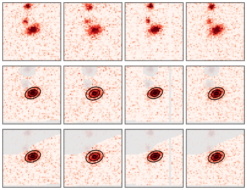
An example set of images and überseg maps are shown in Figure 11. In tests on a simulation with realistically blended galaxies (cf. §6.2), we found a large reduction in the shear biases when using the überseg masking as compared to the ordinary SExtractor segmentation maps. In particular, when using ordinary segmentation maps we found a significant bias of the galaxy shape in the direction toward neighbors. With the überseg masking, such a bias was undetectable.

6 Simulations

Simulations were a crucial part of our shear pipeline development process, providing data with known values of the applied shear for testing the shear estimation code. There is no such absolute calibration source in the real data. In addition to many small targeted simulations designed to answer particular questions about the algorithms, we developed two general purpose simulations that we used extensively to test the shear pipelines.

The first, which we call GREAT-DES, was modeled on the GREAT3 challenge. We used the GREAT-DES simulation to test the accuracy of the shear estimation codes on realistic space-based galaxy images with a realistic range of noise levels and galaxy sizes. As with the GREAT3 challenge, the galaxies were placed on postage stamps, so there were no blending or object detection issues to consider.

The second, which we call the end-to-end simulation, was a high $S/N$ simulation with analytic galaxy models with elliptical isophotes. The motivation with these simulations was to test that various bookkeeping details were implemented correctly, such as the file conventions used by PSFEx, the application of the WCS transformations, and conventions about the origin of the postage stamps in the MEDS files. These are all details that are easy to get wrong, but which can be difficult to notice on noisy data. In these simulations we also tested the efficacy of the überseg masking (c.f. 5.2).

We have found the GalSim (Rowe et al., 2015) image simulation software to be invaluable for this purpose. In particular, its ability to accurately render sheared versions of space-based images using their reimplementation of the SHERA algorithm (SHEar Reconvolution Analysis; Mandelbaum et al., 2012), correctly accounting for the original HST PSF (Bernstein & Gruen, 2014), was particularly important for making the GREAT-DES simulation. The end-to-end simulation relied on GalSim’s ability to generate multiple epochs of the same scene and accurately handle non-trivial WCS transformations for the various exposures.

6.1 GREAT-DES

We used the GREAT-DES simulation to test the precision and accuracy of our shear measurement codes, using DES-tuned sampling of both the population of galaxies (size, shape, morphology) and the observing conditions (PSF ellipticity, noise level). The simulation consists of individual $48\times 48$ pixel postage stamp images. We ignored issues of crowding, bad pixels, and imaging artefacts, but we otherwise attempted to make the images a close approximation to the DES SV data.

We built the GREAT-DES simulation using galaxies from the COSMOS survey (Koekemoer et al., 2007), made available for use with GalSim. Kannawadi et al. (2015) showed that this sample of galaxies is a good representation of galaxy properties, and can be used in shear calibration of lensing surveys to a precision level of $m\!=\!0.01$.

Figure 12: A comparison of the galaxy properties in GREAT-DES (red) and the SV data (blue). The top row shows histograms of $|e|$, $R_{gp}/R_{p}$, and $S/N$ as measured by im3shape. The bottom row shows the dependence of $\langle R_{g}\rangle$, $\langle R_{gp}/R_{p}\ \rangle$, and bulge fraction as functions of $S/N$.

We started with the entire COSMOS sample distributed for use with GalSim  and discarded objects that were flagged as unusable in the GREAT3 challenge (Mandelbaum et al., 2014), which removed about 3% of the objects and left more than 54,000 COSMOS galaxies available for use in the simulation. Next we selected individual galaxies from this set in such a way as to mimic the distribution of galaxy properties found in DES SV data.

For the PSF, we used a Kolmogorov profile with sizes and ellipticities taken to match the range of values present in the SV data. Specifically the PSF size took one of 6 values between 0.8 and 1.3 arcseconds FWHM, and each component $e_{1}$, $e_{2}$ of the shape took one of 4 values from -0.02 to +0.02. Thus, a total of 96 unique PSF images were used in the entire sample. Gaussian noise was added based on the typical noise level observed in SV coadd images.

We then applied a constant shear value within each simulation field, with a magnitude of $|g|=0.05$ and rotated at 8 evenly spaced position angles $\phi$.

Each of the COSMOS galaxies was used hundreds of times, with different noise realizations, different random orientations and different centroid offsets. We did not use 90 degrees rotated galaxy pairs, as has commonly been done for the GREAT challenges (cf. Kitching et al., 2010) to reduce the number of galaxies required to reach a given measurement precision. We instead randomly oriented each galaxy. With this choice, we retained the ability to select subsets of the galaxies according to their measured characteristics. Such selections tends to break up the pairs, which obviates any advantage from using them. More importantly, additive errors can cancel between the pairs of galaxies, which would hide important systematic errors that would yet appear real data. Therefore, we instead use a very large number of galaxies in each field to get to the desired precision on the mean shear. In total, we use 48 million rendered galaxy images.

We developed a DES-specific module for GalSim to store the simulated images directly in MEDS format, so we could run im3shape and ngmix on the resulting MEDS files with minimal modification compared to how we run the code on the data. We did not actually create multiple epochs for this simulation, but it was helpful to use the same file format as the data.

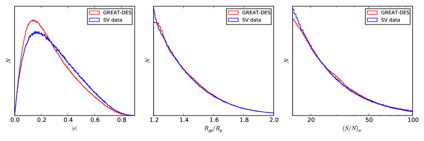
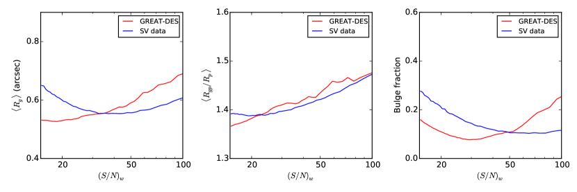
To estimate the level of systematic errors well, we desired the simulation to be closely representative of the data (see e.g. Bergé et al., 2013; Bruderer et al., 2015). To check that we have achieved this goal, we compared the im3shape measurements of relevant galaxy properties in GREAT-DES to those in the SV data. In Figure 12 we show that the distributions of ellipticity, size and $S/N$ are well-matched between the simulation and the data, as is the dependence of $R_{g}$ and $R_{gp}/R_{p}$ as functions of $S/N$. The bulge fraction, estimated by which model im3shape chooses as the better fit, shows systematic disagreement as a functioin of $S/N$, although the overall bulge fraction matches very well: 0.161 and 0.167 for the simulation and the data respectively.

Note that the choice to show im3shape measurements in Figure 12 is arbitrary; the analogous plot of ngmix measurements shows similar agreement, except that there is no estimate of bulge fraction from the ngmix exponential disc model. Also, the im3shape “bulge fraction” should not be considered an estimate of the actual Sérsic index of the galaxies; it is merely a diagnostic measure related to the concentration of the galaxies.

Since ngmix uses an exponential disc model (cf. §7.4.1), and thus has worse model bias for bulge-like galaxies, the discrepancy in the bulge fraction limits our ability to infer what the model bias would be in real data (cf. §8.5). The im3shape shear estimate is based on a bulge-or-disc galaxy model (cf. §7.3.1), which has less overall model bias (Kacprzak et al., 2014), so the discrepancy may have less impact. However, the ability to accurately choose bulge vs. disk is dependent on $S/N$, so our ability to test this aspect of the fitting is also somewhat limited in GREAT-DES.

6.2 End-to-end Simulation

The end-to-end simulation is of an entirely different nature from the GREAT-DES simulation. It is a high $S/N$ simulation used to test various mundane coding details that are easy to mix up, but which can be difficult to verify in noisy data. For the galaxies we used simple exponential disc profiles, which have elliptical isophotes when sheared, and the images were rendered with relatively little pixel noise. The fundamental shape estimation problem is thus straightforward for both algorithms.

The starting point for this simulation was one of the actual MEDS files from the data, along with the corresponding coadd catalogue, the list of single-epoch images that contributed to the coadd image, and the WCS solutions and estimated background maps for each single-epoch image.

Next we built new versions of these single-epoch images using exponential disc galaxies with the same size, flux, ellipticity, and celestial position as the measurements of the real galaxies. We used variable elliptical Gaussian profiles for the PSF, using different parameters for each single-epoch image. The convolved images were rendered at the correct position on each image using the original WCS. With GalSim we applied the Jacobian of the WCS to the surface brightness profile as well, so this important detail was handled correctly. Objects that were deemed to be stars in the original catalogue (based on the SExtractor SPREAD_MODEL being less than 0.003) were drawn as a PSF profile, with the same flux as the original object. Finally, we added the original background sky level to the image, but with relatively small noise so that the faintest galaxies had $S/N>200$.

We then ran these images through the full weak lensing pipelines, starting with SExtractor and PSFEx to estimate the PSF model, then building a MEDS file, and finally running im3shape and ngmix. The resulting measured shape estimates were then compared to the true shapes of the simulated galaxies, which were expected to match to quite high precision, given the nature of the simulation.

The end-to-end simulation was successful in finding several bugs in various parts of the shear pipeline. However, the most notable result from this process was the development of the überseg mask (cf. §5.2). These tests revealed significant biases from the masking procedure we had been using, involving just the SExtractor segmentation maps. When a galaxy had a bright neighbor on the same postage stamp, light from the neighbor that was just outside the segmentation map was being included as part of the fit, thus significantly biasing the inferred shapes in the direction of the neighbor.

Switching to the überseg mask made a big difference; we found the measured shapes were then much closer the true values. We found there was still a small effect from neighbors, which amounted to a slight increase in the effective shape noise for such objects, but we no longer detected any systematic bias in the shape estimates due to unmasked flux from neighboring objects.

7 Shear Measurement

We used two different shear measurement codes for this study: im3shape and ngmix, both of which are based on model-fitting. im3shape performs a maximum likelihood fit using a bulge-or-disc galaxy model (cf §7.3.1). ngmix uses an exponential disc model, exploring the full $N$-dimensional posterior likelihood surface with an informative prior applied on the ellipticity (cf. §7.4.1).

With both shear methods we used the PSFEx models of the PSF detailed in §4.3, although the way the PSF model was used differed. PSFEx produces a 2-D image of the PSF profile at the location of each galaxy. With im3shape we resampled the PSF image to a higher resolution grid and performed the convolution with the galaxy model via FFT. With ngmix, we fit 3 free elliptical Gaussians to the PSF image and performed an analytic convolution with the galaxy model, which was also approximated as a sum of Gaussians, resulting in very fast model creation.

Finally, with both shear codes we used the MEDS files described in §5 to constrain the galaxy models, using pixel data from the original single-epoch images rather than using the coadd image, which we only used for object detection.

We discuss the details of the multi-epoch fitting process in the next section, §7.1. In §7.2, we define what we mean by signal-to-noise. The details of the im3shape and ngmix algorithms are given in §7.3 and §7.4. Finally, our strategy for blinding the shear estimates is described in §7.5.

7.1 Multi-epoch Fitting

The typical method for dealing with multiple exposures of a particular patch of sky is co-addition of images (also known as “stacking”; cf. Fu et al., 2008). However, co-addition can be problematic, since it necessarily loses information and imparts non-trivial, spatially correlated noise into the final image. Furthermore, as each CCD covers a finite region of sky, addition of a finite number of CCD images results in discontinuities in the PSF at image boundaries (cf. Jee et al., 2013 for a discussion of this effect). A more optimal method for fitting a collection of images is to simultaneously fit all independent pixel data, as also advocated by Heymans et al. (2012b). We call this process multi-epoch fitting.

Multi-epoch fitting requires some additional complexity in the fitting process, as we must use the correct PSF and WCS information for each image, rather than a single function for each as would be sufficient to process a coadd image.

In order to simplify the bookkeeping to process the multi-epoch and multi-band DES data, we used the Multi-Epoch Data Structures described in §5. Each observation of a particular galaxy experiences a different PSF, and the local image coordinates are related to celestial coordinates via a different WCS transformation. This information was stored in the MEDS file and used during modeling.

For both codes (ngmix and im3shape) the model for a given set of galaxy parameters was generated in celestial coordinates. For ngmix, we modeled the PSF in celestial coordinates as well, and convolved it with the galaxy model analytically. We then compared this model to the observed data using the WCS transformation. For im3shape we modeled the galaxy and PSF in image coordinates and convolved via fast Fourier transform (FFT).

7.2 Signal-to-noise Ratio

Before we describe the algorithms we used for measuring shapes, it is worth describing in detail what we mean by the signal-to-noise ratio ($S/N$). This will be relevant both in the next section (in particular §7.3.2, where we discuss how im3shape calibrates the shear bias) and in later sections such as §8.3, where we test that the shear is independent of $S/N$, and §9.1, where we use $S/N$ while selecting galaxies for the final shear catalogues.

There is no single definition for the $S/N$ of an image or a surface brightness profile. Rather, a $S/N$ is only well defined for a single measured value – some statistic calculated from the image or profile. Given some such statistic $x$, the $S/N$ is typically defined as that value (either the measurement or the true value) divided by the square root of its variance

$$S/N\equiv\frac{x}{\sqrt{\textrm{Var}(x)}}.$$ (7.1)

One of the standard $S/N$ measures is the so-called “optimal” $S/N$ estimator. One can show that among all statistics that are linear in the pixel values $I_{p}$,

$$\hat{I}_{w}=\sum_{p}w_{p}I_{p},$$ (7.2)

the one with the highest expected $S/N$ has weights $w_{p}=\langle I_{p}\rangle/\sigma_{p}^{2}$, where $\sigma_{p}^{2}$ are the estimated variances in each pixel.

In practice, one does not know the true expectation value of the surface brightness profile, $\langle I_{p}\rangle$, so typically one uses the best-fitting model of the galaxy, which we call $m_{p}$, as part of the weight. The $S/N$ of this statistic is thus estimated as

$$(S/N)_{w}=\frac{\sum_{p}m_{p}I_{p}/\sigma_{p}^{2}}{\left(\sum_{p}m_{p}^{2}/\sigma_{p}^{2}\right)^{1/2}}.$$ (7.3)

This is the $S/N$ measure used by GREAT3 (Mandelbaum et al., 2014), for example.

A drawback of this estimator is that it is not independent of an applied shear. Galaxies that look similar to the PSF will have a higher measured $(S/N)_{w}$ than galaxies with a different size or shape. The PSF essentially acts as a matched filter for these galaxies. This means that $(S/N)_{w}$ is not invariant under an applied gravitational shear.

If the PSF is approximately round, as is the case for our data, then more elliptical galaxies will have a lower estimated $(S/N)_{w}$ than round galaxies (holding flux constant). Thus if galaxies are selected according to their measured $(S/N)_{w}$, the resulting galaxy catalogue will have a selection bias towards round shapes, which will bias the overall mean shear.

One solution to this potential systematic error is to use a $S/N$ estimator that is not biased with respect to an applied shear. There are a number of choices one could make for this. We choose to calculate the $(S/N)_{w}$ that the galaxy would have had if it and the PSF were round.

That is, we take the model of the galaxy profile and apply a shear such that its ellipticity becomes zero. We do the same for the PSF, convolve these two profiles together, and then integrate over the pixels. The resulting $m^{r}_{p}$ values are the intensities we predict would have been observed if both the galaxy and the PSF had been round. We then use these values for both the model $m_{p}$ and the intensity $I_{p}$ in equation 7.3, as the actual data are no longer appropriate for this counterfactual surface brightness profile. The “roundified” $S/N$ estimator is then

$$(S/N)_{r} =\frac{\sum_{p}m^{r}_{p}m^{r}_{p}/\sigma_{p}^{2}}{\left(\sum_{p}(m^{r}_{p})^{2}/\sigma_{p}^{2}\right)^{1/2}}$$

$$=\left(\sum_{p}(m^{r}_{p})^{2}/\sigma_{p}^{2}\right)^{\!\!1/2}.$$ (7.4)

We find both measures of the signal-to-noise useful in different contexts. For ngmix, we use $(S/N)_{r}$ for the reasons described here; we find significantly smaller selection biases when we use $(S/N)_{r}$ to select galaxies for shear measurement, as compared to using $(S/N)_{w}$.

For im3shape, we find that the noise bias calibration (cf. §7.3.2) is more accurate using $(S/N)_{w}$ than $(S/N)_{r}$, presumably because the noise bias is more directly related to the signal-to-noise of the actual galaxy than to that of a counterfactual round version of the galaxy. Thus, the “noise bias” calibration in fact also approximately calibrates the selection bias resulting from using $(S/N)_{w}$. This is therefore the appropriate $S/N$ measure to use for selecting galaxies for the final im3shape catalogue.

7.3 Shear Measurements with im3shape

im3shape is a maximum-likelihood model-fitting code, which we used to fit de Vaucouleurs bulge and exponential disc components to galaxy images. The code was described in Zuntz et al. (2013), where its performance on GREAT08 and its known biases were characterized.

We have slightly modified the model described therein, improving both its stability and its performance on the tests detailed in this paper (cf. §8). Previously each galaxy was modeled as the sum of two components, a bulge and a disc. In this paper, we fit each galaxy twice: once as a pure bulge and once as a pure disc. For shear estimation, we used the model with the higher likelihood, unless that model was flagged as a bad fit (cf. §7.3.3). If both models were flagged the galaxy was excluded from the catalogue.

We found this “bulge or disc” scheme to be much more robust on simulations of realistic galaxies. This scheme produced good model fits in almost all cases, whereas with the previous “bulge plus disc” scheme we frequently found the best fit model was unphysical, with highly negative-flux components.

The parameters of the best-fitting model were found using the numerical optimizer LevMar (Lourakis, 2004), which is an implemention of the Levenberg-Marquardt algorithm (Levenberg, 1944; Marquardt, 1963), iterating towards a model image which minimizes the $\chi^{2}$ with the data image.

For the SV data, we ran im3shape on $r$-band images only. With the future data we plan to test fitting multiple bands simultaneously with marginalized relative amplitudes.

We made a number of additions to the original code presented in Zuntz et al. (2013); in this section we briefly review the code and its methodology, with particular focus on these changes.

The complete code with all the changes described below is available for download. One particularly useful infrastructure improvement was the implementation of a Python interface to the existing C functions. We used the Python interface to load data from MEDS files (via the meds module), select exposures, mask images, and compute most of the diagnostic information described in §7.3.3 below.

The biggest change we made to im3shape was the addition of a new model which fits multiple exposures of the same galaxy simultaneously. We now define our model parameters in a celestial coordinate system: a local tangent plane centred at the nominal Right Ascension and Declination of the galaxy. This model is then constrained by the pixel data from each epoch where the galaxy was observed, as discussed in §7.1.

7.3.1 Bulge or disc model

Each galaxy model was defined by six varied parameters: the amplitudes of either the bulge or disc components ($A_{b},A_{d}$), a centroid relative to the nominal detection position ($\delta u,\delta v$), an ellipticity ($e_{1},e_{2}$), and a half-light radius ($r$).

To compute the likelihood of a particular model for a given galaxy observed on a number of individual exposures, we used the local affine approximation to the WCS for each postage stamp (stored in the MEDS file) to transform these parameters into each image’s local pixel coordinate system. Schematically,

$$\left\{\delta u,\delta v,e^{c}_{1},e^{c}_{2},r^{c}\right\}\rightarrow$$

$$\qquad\bigl{[}\left\{\delta x,\delta y,e^{p}_{1},e^{p}_{2},r^{p}\right\}_{\textrm{Image 1}},$$

$$\qquad~{}\left\{\delta x,\delta y,e^{p}_{1},e^{p}_{2},r^{p}\right\}_{\textrm{Image 2}},...\bigr{]}$$ (7.5)

where ^c indicates the parameters in celestial coordinates ($u,v$) and ^p indicates the transformed parameters in pixel coordinates ($x,y$). The amplitudes do not require any transformation, since the MEDS files have already put the postage stamps on the same photometric system.

Given the appropriate parameters for each postage stamp, we then built the galaxy models in pixel coordinates, each convolved by the correct PSF for that stamp, and computed a $\chi^{2}$ of the model relative to the data, using the correct pixel noise. The total $\chi^{2}$ from all the postage stamps then gave us the final likelihood to use for that set of model parameters. We then iterated to find the maximum likelihood parameters for each galaxy. The maximum likelihood was typically found in less than 50 iterations. At 150 iterations, we stopped the algorithm and declared failure.

The Levenberg-Marquadt code that we used to find the maximum likelihood, LevMar, does not directly handle problems where different weights are applied to each data point. The straightforward fix for this is to scale both the observed intensity $I_{p}$ and the model $m_{p}$ by the standard deviation of the intensity $\sigma_{p}$ before passing them to LevMar:

$$I^{\mathrm{LM}}_{p} =I_{p}/\sigma_{p}$$

$$m^{\mathrm{LM}}_{p} =m_{p}/\sigma_{p}.$$ (7.6)

This maintains the $\chi^{2}$ per pixel that the LevMar algorithm uses as its objective function. The estimates of $\sigma_{p}$ came from the weight map (as $\sigma_{p}^{-2}$) provided with the images.

Figure 13: Shear bias for im3shape measurements on the GREAT-DES simulation: multiplicative bias (left) and PSF leakage (right), as functions of the measured $(S/N)_{w}$ and $R_{gp}/R_{p}$. The fits, which are used to calibrate the shear estimates on the data, are smooth functions in both of these variables. Solid lines show the fits vs $(S/N)_{w}$ at particular choices of $R_{gp}/R_{p}$.

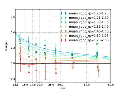
7.3.2 Shear calibration

A significant problem with maximum likelihood shear estimators is that the peak of the likelihood distribution is not an unbiased estimator of the shear in the presence of noise (Refregier et al., 2012; Kacprzak et al., 2012). The fitted model parameters are a non-linear function of pixel intensities affected by Gaussian noise, resulting in noise bias in the estimated shear values. The im3shape algorithm, being a maximum likelihood estimator, is known to suffer from this effect.

In addition, we found a small selection bias, which is introduced by using recommended im3shape flags (cf. §7.3.3) and the selection based on galaxy size and $S/N$ (cf. §9.1). We also expect a small amount of model bias due to realistic galaxies not always being well fit by our bulge-or-disc model. This model bias is expected to be small compared to the requirements (Kacprzak et al., 2014).

To account for all of these sources of error in our shape measurements, we calculated bias corrections of the form shown in equation 3.4. Specifically, we fit for $m$ and $\alpha$ as functions of $(S/N)_{w}$ (defined in equation 7.3) and $R_{gp}/R_{p}$ (the FWHM of the PSF-convolved galaxy divided by the FWHM of the PSF) on simulated data from the GREAT-DES simulation (cf. §6.1). We ran im3shape on the simulated data in the same way as we do on the DES data, including the same choices of input parameters.

In principle, the two multiplicative terms, $m_{1}$ and $m_{2}$ should be treated as independent biases. In practice, however, when averaged over many galaxies we find virtually no difference between the two. As such, we correct both $e_{1}$ and $e_{2}$ by the average $m=(m_{1}+m_{2})/2$.

We fit both $m$ and $\alpha$ as two-dimensional surfaces in the $S/N$ and size parameters. Due to the complicated structure of this surface, we fit $m$ with 15 terms of the form $(S/N)_{w}^{-x}(R_{gp}/R_{p})^{-y}$, where $x$ and $y$ are various powers ranging from 1.5 to 4. To control overfitting, we used a regularization term in the least-square fit and optimized it such that the fitted surface has a reduced $\chi^{2}=1$. A similar procedure was applied to $\alpha$, where we used 18 parameters in the fit. In Figure 13 we show these fits as curves in $(S/N)_{w}$ in bins of $R_{gp}/R_{p}$. However, the actual functions are smooth in both parameters.

We checked if our calibration is robust to the details of this model by (1) varying the number of terms in the basis expansion and (2) splitting the training data into halves. For both tests the changes in the mean multiplicative and additive corrections applied to the SV data did not vary by more than 1%.

In §7.2, we mentioned that $(S/N)_{w}$ is a biased measure of $S/N$ with respect to shear, so if it is used to select a population of galaxies, it will induce a selection bias on the mean shear. $R_{gp}/R_{p}$ similarly induces such a bias. Thus, when we bin the shears by these quantities to construct the calibration functions, there is a selection bias induced in every bin. The scale of selection bias reaches $m\simeq-0.05$ for the most populous bins. This is not a problem for the correction scheme so long as the overall selection is also made using these same quantities. In that case, the shear calibration automatically accounts for the selection bias in addition to the noise bias.

We tried using $(S/N)_{r}$ in the calibration model rather than $(S/N)_{w}$ to help reduce the level of the selection bias in each bin, but we found that it does not perform as well as using the standard $(S/N)_{w}$. Perhaps not surprisingly, the noise bias seems to be more related to the $S/N$ of the actual galaxy than it is to the counterfactual round version of the galaxy used for $(S/N)_{r}$. In future work, it would be interesting to seek an effective shear calibration scheme that disentangles noise and selection biases, but we have not found one yet.

We used these fits to estimate the multiplicative and additive corrections to use for every galaxy in the im3shape catalogue. However, it should be stressed that this bias estimate is itself a noisy quantity, being based on noisy estimates of the size and $S/N$. Therefore one should not directly apply the correction to each galaxy individually. Rather, the mean shear of an ensemble of galaxies should be corrected by the mean shear bias correction of that same ensemble (cf. §9.2).

Note that a selection bias can appear whenever a subset of galaxies is selected from a larger sample. In the cosmological analysis, we apply recommended im3shape flags, cut on $R_{gp}/R_{p}$ and $(S/N)_{w}$, and then typically split the galaxies into redshift bins. The redshift selection in particular is not used in the shear calibration process, so it is possible for there to be uncorrected selection biases in the different redshift bins. In §8.5, we test that the shear calibration nevertheless performs well in this scenario by applying the same selection procedure to the GREAT-DES simulation. There we demonstrate that all biases are removed to the required tolerance level in all redshift bins.

7.3.3 Diagnostics

After performing the shape measurement, we generated a large suite of diagnostic information based on the results of the fits to help identify objects that potentially should not be used for weak lensing. Many objects showed evidence of imaging artefacts or some other problem that violates the assumptions we have made in the model, so we wanted to be able to remove these objects from the final shear catalogue.

We distinguished two types of flags: “error” flags, which identify objects that should definitely be removed from any analysis, and “info” flags, which identify objects that may be somewhat contaminated, but which may have some value depending on the science application. Most of the info flags are derived by examining histograms of the relevant parameters and flagging extreme tails.

The full listing of im3shape flags is given in Appendix B.1. In §9.1, we will detail the final selection criteria that we recommend for the im3shape catalogue, which will include both ERROR_FLAG==0 and INFO_FLAG==0. Moving to a less restrictive selection should only be done after carefully testing for the possibility of increased systematic errors.

7.3.4 Galaxy weights

We assigned a weight to each shear measured by im3shape based on an estimate of the total shear uncertainty including both shape noise $\sigma_{\textsc{sn}}$ (the standard deviation of the intrinsic ellipticities) and measurement uncertainty $\sigma_{e}$:

$$w=\frac{1}{\sigma_{\textsc{sn}}^{2}+\sigma_{e}^{2}}.$$ (7.7)

The LevMar Levenberg-Marquardt implementation we used produces an estimate of the parameter covariance for each galaxy as a by-product of optimization, but we did not use this estimate to give us weights, for two reasons. First, we found it to show rather wide scatter when compared to MCMC tests, often showing spurious parameter covariances. Second, our physical parameters are a non-linear function of the numerical parameters in some regimes, as discussed in Zuntz et al. (2013).

To estimate the appropriate weight for each galaxy, we instead used the measured shears from the GREAT-DES simulation. We grouped galaxies in bins of $(S/N)_{w}$ and $R_{gp}/R_{p}$. We then measured the width of the distribution of ellipticities in each bin, both by fitting a Gaussian to a histogram of the distribution and by measuring the sample variance directly. The larger of the two variance estimates was taken, and the weight was then given by the inverse variance.

We also imposed a maximum weight set by the mean variance of all high-$S/N$ bins. Otherwise spuriously low variance estimates in some sparsely populated bins resulted in very high weight values for those bins.

7.4 Shear Measurements with ngmix

The code ngmix is a general tool for fitting models to astronomical images (Sheldon, 2014). The code is free software, and is available for download.

In ngmix  both the PSF profile and the galaxy are modeled using mixtures of Gaussians, from which the name ngmix is derived. Convolutions are thus performed analytically, resulting in fast model generation as compared to methods that perform the convolution in Fourier space.

7.4.1 Exponential disc model

For the galaxy model, ngmix supports various options including exponential discs, de Vaucouleurs profiles (de Vaucouleurs, 1948), and Sérsic profiles (Sérsic, 1963), all of which are implemented approximately as a sum of Gaussians using the fits from Hogg & Lang (2013). Additionally, any number of Gaussians can be fit, either completely free or constrained to be co-centric and co-elliptical. For the DES SV catalogues, we used the exponential disc model for galaxies.

Using this simple disc model resulted in detectable model bias (cf. §8.5). In simulations, we found this model bias was reduced when using a more flexible model, but the more flexible model was not implemented for real survey data in time for this release. We will explore improved modeling in detail for future DES analyses.

We constructed the model in celestial coordinates and fit it to multiple epochs and bands simultaneously (cf. §7.1). The centre, size and ellipticity were set to be the same for all bands and epochs, but the flux was allowed to vary between bands. For this study we combined bands $r,i,z$, resulting in eight free parameters:

• $u_{c},v_{c}$, the object centre in celestial coordinates, relative to the fiducial centre from the coadd object catalogue. The units are arcseconds.

• $e_{1},e_{2}$, the ellipticity.

• $T$, the area of the object, defined in terms of the unweighted moments of the Gaussian mixture $T=\langle x^{2}\rangle+\langle y^{2}\rangle$. The units are arcseconds squared.

• $F_{k}$, the flux in each of the $r,i,z$ bands.

7.4.2 Image fitting

The ngmix code supports multiple paradigms, all of which were used in the current analysis:

• Exploration of the full likelihood surface for a given set of model parameters with a Markov Chain Monte Carlo (MCMC) scheme, using either the standard Metropolis-Hastings algorithm (MH; Metropolis et al., 1953) or the recently introduced affine invariant method (Goodman & Weare, 2010; Foreman-Mackey et al., 2013). The model can be fit directly to the pixel data, or it can include convolution by a point-spread function (PSF).

• Maximum-likelihood fitting using any of a variety of function minimizers. We used Levenberg-Marquardt (LM; Levenberg, 1944; Marquardt, 1963) as well as the method of Nelder & Mead (1965) (NM) in this work. The model can be fit directly to the pixel data, or it can include convolution by a PSF.

• Expectation Maximization (EM; Dempster et al., 1977), fitting directly to the pixels only. This method is used for PSF fitting.

For PSF measurement, the EM code was used, with three completely free Gaussians. EM is a good choice for PSF measurement, since it is extremely stable even with many components. By allowing all components to be completely free, the off-centre PSF components that are occasionally found in the SV PSF images were fitted without instability.

We chose to handle the WCS information by projecting each pixel into celestial coordinates and building both the galaxy and PSF models in that coordinate system.

Our procedure for fitting the galaxy shapes involves a number of steps:

1. Estimate a flux for the object by fitting the PSF model to the galaxy with a single free parameter, which is the overall normalization (keeping the centroid fixed at its fiducial value).

2. Run NM to find the maximum likelihood model, guessing the flux from the result of step 1, and guessing the size to be the typical seeing size. We find NM to be more robust than LM for this fit.

3. Run LM starting from the maximum likelihood model to estimate the covariance matrix, since NM does not produce one. Relatively few evaluations are made in this step.

4. Run an MCMC chain with MH using the maximum likelihood position as a starting guess and the covariance matrix as a proposal distribution. We run a few thousand burn-in steps, followed by a few thousand post-burn-in evaluations. If the acceptance rate is outside the range $[0.4,0.6]$ we reset the proposal distribution based on the covariance matrix from previous MH run, and run a new burn-in and post-burn in. If the acceptance rate remains outside the desired range we try again up to four times. These bounds on the acceptance rate are somewhat arbitrary, but for our problem we found that rates above 0.6 result in highly correlated chains, and lower than 0.4 can result in a poorly sampled peak.

7.4.3 Shear estimation

Multiple methods are supported for shear measurement, but for this study we adopted the “lensfit”-style method, based on the work of Miller et al. (2007). We found our implementation of this method to be sufficiently accurate for the precision of our current data set; for this study ngmix measurements were instead limited by the use of an overly simple exponential disc model for galaxies (cf. §8.5).

The lensfit method involves multiplication by a prior on the distribution of galaxy ellipticities when estimating the expectation value of the ellipticity for each galaxy.

$$\langle e_{\mu}\rangle =\frac{\int\mathcal{L}(\mbox{\boldmath$e$})p(e)e_{\mu}\mathrm{d}\mbox{\boldmath$e$}}{\int\mathcal{L}(\mbox{\boldmath$e$})p(e)\mathrm{d}\mbox{\boldmath$e$}}$$ (7.8)

$$\simeq\frac{\sum_{j}p(e^{j})e^{j}_{\mu}}{\sum_{j}p(e^{j})},$$ (7.9)

where $\mathcal{L}(\mbox{\boldmath$e$})$ is the likelihood and $p(e)$ is the prior on the galaxy shapes. We approximate the integral over the likelihood with the sum of points from an MCMC chain. The index $\mu$ takes values 1,2 for each ellipticity component such that $\mbox{\boldmath$e$}=(e_{1},e_{2})$; the ellipticity magnitude is given by $e$.

Multiplying by an ellipticity prior reduces the effects of noise, which broadens and distorts the likelihood surface. However, application of the prior also biases the recovered shear, in effect reducing the “sensitivity” of the shear estimate. Miller et al. (2007) derive a measure of the sensitivity of this estimator to a shear $g$, which is approximately given for each component by:

$$s_{\mu}\equiv\frac{\partial\langle e_{\mu}\rangle}{\partial g_{\mu}} \simeq 1-\left[\frac{\int\left(\langle e_{\mu}\rangle-e_{\mu}\right)\mathcal{L}(\mbox{\boldmath$e$})\frac{\partial p}{\partial e_{\mu}}\mathrm{d}e}{\int\mathcal{L}(\mbox{\boldmath$e$})p(e)\mathrm{d}e}\right]$$

$$\simeq 1-\left[\frac{\sum_{j}\left(\langle e_{\mu}\rangle-e^{j}_{\mu}\right)\frac{\partial p}{\partial e_{\mu}}}{\sum_{j}p(e^{j})}\right].$$ (7.10)

No expression was formally derived by Miller et al. (2007) for the mean of the shear field acting on an ensemble of galaxies; however, it was proposed to use the same formula as derived for a constant applied shear:

$$g_{\mu}=\frac{\sum_{i}\langle e^{i}_{\mu}\rangle}{\sum_{i}s^{i}_{\mu}},$$ (7.11)

where the index $i$ runs over all galaxies in the measurement. In practice we also apply weights in both sums,

$$w=\frac{1}{2\sigma_{\textsc{sn}}^{2}+C_{1,1}+C_{2,2}},$$ (7.12)

where $\sigma_{\textsc{sn}}$ is the shape noise per component, which we have calculated to be 0.22 based on fits to COSMOS galaxies (cf. §7.4.4), and $C_{i,j}$ are elements of the 2x2 ellipticity subset of the covariance matrix produced by ngmix.

The sensitivities in equation 7.4.3 do not transform as polarizations. Thus for practical shear measurements, such as tangential shear or two-point functions, which require rotation of the ellipticities, we chose to use a scalar sensitivity for each galaxy that is the mean of its two components.

7.4.4 Ellipticity prior

The lensfit method requires as input a prior on the shapes of galaxies, $p(e)$. The prior must be continuous for $e_{1},e_{2}$ in the unit circle in order to evaluate the derivatives in equation 7.4.3.

In simulations, we found that the accuracy of the shear recovery was sensitive to the details of the ellipticity prior. For example, we ran the shear code on the GREAT-DES simulation presented in §6.1 using a prior with intrinsic variance in ellipticity 35% higher than the true variance, and found the multiplicative bias increased by $(1.3\pm 0.2)$%.

For application to real data, we based our prior on the ellipticities of Sérsic model fits to COSMOS galaxies, as released by the GREAT3 team (Mandelbaum et al., 2014). We fit the observed distribution to a simple model

$$p(e) =2\pi eA~{}\frac{\left(1-\mathrm{exp}\left[\frac{e-1}{a}\right]\right)}{(1+e)\sqrt{e^{2}+e_{0}^{2}}}~{}c(e)$$ (7.13)

$$c(e) =\frac{1}{2}\left(1+\mathrm{erf}\left[\frac{e_{cut}-e}{\sigma_{e}}\right]\right).$$ (7.14)

This model is a modified version of that introduced in Miller et al. (2013). Note in particular the cutoff at high ellipticities achieved by using an error function. We found this formula improved the fit to the distribution of ellipticities.

Figure 14: Distribution of shapes for COSMOS galaxies, selected as described in the text. The model fit was used as a prior for the ngmix shear analysis.

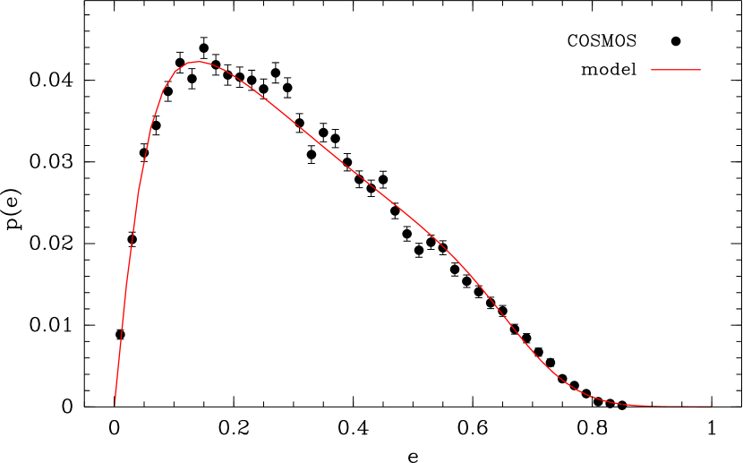
We fit this model to the ellipticities of COSMOS galaxies selected to fall in a range of size and flux that corresponds to the galaxy population seen in our data. A comparison between the measured $p(e)$ and the fit model is shown in Figure 14. The best-fitting parameters are given in Table 1.

Parameter	Fit Value
$A$	$0.025\pm 0.002$
$a$	$2.0\pm 0.2$
$e_{0}$	$0.079\pm 0.003$
$e_{cut}$	$0.706\pm 0.004$
$\sigma_{e}$	$0.125\pm 0.006$

Table 1: Parameters for the ellipticity prior used with the ngmix shear code, with best-fitting values for the distribution of shapes of COSMOS galaxies.

We used this same prior for all galaxies, but the distribution of COSMOS galaxy shapes depends on redshift. However, for this study we found that the uncertainties due to the redshift dependence of the shape distribution were sub-dominant to model bias for ngmix (cf. §8.5).

7.5 Blinding

We blinded the shape catalogues from both pipelines before they were used for any tests or SV science papers. We did this to prevent the experimenter bias effect, wherein researchers work harder on finding bugs, tuning methodology, etc. when results are inconsistent with a previous experiment, or otherwise do not match expectations, than when they do match (cf. Klein & Roodman, 2005).

We blinded the SV shear catalogues by scaling all measured shears by a secret factor generated by an algorithmic, but unpredictable, process (using an MD5 hash of a code phrase) to be between $0.9$ and $1.0$. This unknown scaling meant that it was harder for DES members to, for example, accidentally tune results to get the $\sigma_{8}$ value predicted by Planck. We only unblined the catalogues after the analysis for a given paper was finalized.

This was a gentle blinding approach that was appropriate for the relatively loose statistical constraints that will come from SV data. It has the useful feature that, being linear, correlation tests on it such as those listed in this paper remain valid. It has a significant downside in that it is asymmetric - unblinding could only increase the measured $\sigma_{8}$, so the potential for bias was still present. We will consider new blinding methodologies for future data.

8 Tests of the Shear Measurements

We developed an extensive test suite to check that the shear catalogues do not have significant systematic errors that would adversely affect weak lensing science. While there is no way to definitely prove that the shear catalogues are free of all possible systematic errors, there are many tests that can reveal systematic errors that might be present in the data. These tests were formulated as “null tests”, which should have zero signal in the absence of systematic errors. Most of our null tests were similar to ones that have been performed in previous analyses (cf. e.g. Jarvis et al., 2003; Schrabback et al., 2010; Velander et al., 2011; Heymans et al., 2012b; Jee et al., 2013; Kuijken et al., 2015).

These null tests can be broken up into several broad categories.

1. Spatial tests to check for systematic errors that are connected to the physical structure of the camera. Examples of these are errors in the WCS correction, including effects like edge distortions or tree rings (Plazas et al., 2014), and errors related to features on the CCDs such as the tape bumps. (§8.1)

2. PSF tests to check for systematic errors that are connected to the PSF correction. This includes errors due to inaccurate PSF modeling as well as leakage of the PSF shapes into the galaxy shape estimates. (§8.2)

3. Galaxy property tests to check for errors in the shear measurement algorithm related to properties of the galaxy or its image. This can include effects of masking as well, which involve the other objects near the galaxy being measured. (§8.3)

4. B-mode statistics to check for systematic errors that show up as a B-mode signal in the shear pattern. The gravitational lensing signal is expected to be essentially pure E-mode. Most systematic errors, in contrast, affect the E- and B-mode approximately equally, so the B-mode is a direct test of systematic errors. (§8.4)

5. Calibration tests to check for systematic errors that affect the overall calibration of the shears. If all of the shear values are scaled by a constant factor, most null tests remain zero (if they were zero to start with). Furthermore, there are no known absolute shear calibration sources that we can use to calibrate our results. For these reasons it can be hard to tease out errors in the calibration from the data. However, we can use simulated data where the true shear is known to check that we recover the correct values. (§8.5)

6. Cross-catalogue comparisons to check that the two shear catalogues are consistent with each other. Because we have two shear catalogues available for testing, we can check that the two give consistent results, thus potentially uncovering problems that may be in one shear catalogue but not the other (or have different levels in each). Considering the large differences between the ngmix and im3shape codes, these are non-trivial tests. (§8.6)

Figure 15: Whisker plots of the mean shear binned by position in the focal plane for im3shape (left) and ngmix (right). As in Figure 9, the length of each whisker is proportional to the mean shear, and the orientation is aligned with the direction of the ellipticity. A 1% whisker is shown for scale in the lower left.

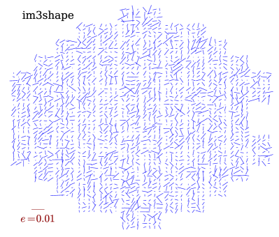
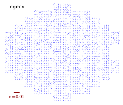
One caveat to keep in mind with the various null tests is that we do not necessarily expect the overall mean shear to be precisely zero. The SV region is small enough that the rms value of the mean shear due to cosmic variance is expected to be about $4\times 10^{-4}$. In fact, the overall mean shear is measured to be

im3shape $$\begin{array}[]{l}\langle e_{1}\rangle=0.1\times 10^{-4}\\ \langle e_{2}\rangle=6.8\times 10^{-4}\end{array}$$

ngmix $$\begin{array}[]{l}\langle e_{1}\rangle=-0.4\times 10^{-4}\\ \langle e_{2}\rangle=10.2\times 10^{-4}.\end{array}$$

These values are both about $2\sigma$ from zero given the expected cosmic variance, so it may be due to an additive systematic error affecting both codes. However, the fact that they roughly agree with each other suggests at least the possibility that it could be a real cosmic shear signal. In any case, each of the null tests look for variations relative to this overall mean shear to find dependencies that may indicate systematic errors.

In §8.1 – §8.6 we show the results of our null tests in each of the above categories. In §8.7 we summarize these results and tries to quantify the total possible systematic errors that may be present in the shear catalogues.

8.1 Spatial Tests

There are many potential sources of systematic error related to the camera and telescope optics that can cause a spatial dependence of the shear with respect to the camera’s field of view. The telescope distortion pattern and some of the optical aberrations are essentially static in time. The CCDs have bad columns and other defects, including the tape bumps mentioned in §4.2. There are also distortion effects at the CCD edges due to the electric field lines becoming non-parallel as well as tree ring distortion patterns due to doping variations in the silicon (Plazas et al., 2014).

8.1.1 Position in the field of view

To check that we have adequately corrected for effects that are connected with the telescope and camera, or that they are small enough to ignore, we binned the shear spatially with respect to the field of view.

In Figure 15 we show the mean shear as a function of position on the focal plane for both im3shape (left) and ngmix (right). Each whisker represents the mean shear of all galaxies that were ever observed in that area of the focal plane. As our shear measurements used information from multiple epochs, each measurement contributed to this plot multiple times: once for each single-epoch observation of that galaxy.

This figure is similar to Figure 9, in which we showed the residual PSF pattern as a function of position on the focal plane. These plots are noisier due to the shape noise of the galaxies, but there is a hint of the same radial patterns that were seen for the PSF residuals, especially in the ngmix results, which are slightly less noisy due to the higher number of galaxies in the catalogue. This is not surprising; we expected these PSF interpolation errors to leak into the galaxy shapes.

8.1.2 Position on CCD

If we bin the shears by their column number, irrespective of the CCD number, as shown in Figure 16, we can see the effect of something known as “edge distortion” (Plazas et al., 2014). This is where the electric field lines in the detector become slightly non-parallel near the edges of the CCDs. The cross section of the pixels becomes rectangular, elongated in the direction towards the edge of the CCD. Plazas et al. (2014, their Figure 6) showed that this effect led to photometric biases of $\sim 20$ mmag at $\sim 30$ pixels from the edge of the CCDs. Since flux and shape respond to the astrometric variation at the same order, this implies that we should expect shape residuals of about $\delta e_{1}\sim 0.02$ near the edge of the CCDs.

Figure 16: The mean shear $\langle e_{1}\rangle$ (blue) and $\langle e_{2}\rangle$ (green) for ngmix, binned by column number $X$; $X$ runs along the readout rows of the CCDs. (The corresponding plot for im3shape looks similar but noisier.) The bottom panel shows the same data blown up near the left and right edges to highlight the effect of the edge distortion. We mask the 15 columns along each edge where the distortion is strongest, but there is still a slight bias in the $e_{1}$ component of the shears up to 40 pixels from the edge.

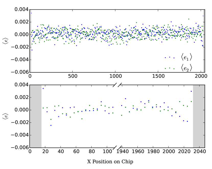
In Figure 16 we show the mean shape measured by ngmix binned by column number. As we do not measure the single-epoch shape, any effect on the shapes has been reduced by a factor of about 10, the number of single-epoch exposures of each galaxy. So we might expect a signal of $\langle e\rangle\sim 0.002$. There does seem to be a slight effect visible in Figure 16 at this level for $e_{1}$, although it is not highly significant. The effect of the edges is even less evident when binning by the row number (not shown).

To quantify how much this edge effect might impact the overall shear signal, we estimated that the effect is only significant for about 20 pixels on any edge. This is a fraction of $40/2048+40/4096=0.015$ of the area. Galaxies have $\sim$ 10 chances to fall in this area, so about 15% of the galaxies may have a spurious shear of $\sim 0.002$. The net additive systematic shear from this effect is thus about $c_{\mathrm{rms}}=8\times 10^{-4}$. This is well below the requirements on additive systematic errors given by equation 3.11, $c_{\mathrm{rms}}<2\times 10^{-3}$; however, it is not below the expected requirements for DES 5-year data. Therefore, we plan to remove this effect directly in the astrometry solution in future DES data analyses.

8.1.3 Tangential shear around field centres

The telescope distortion pattern is approximately a fifth order radial function centred near the centre of the field of view. If it is not corrected it can induce spurious shears oriented either radially or tangentially relative to the field centres. We looked for this effect by measuring the tangential shear pattern around the set of field centres; essentially this is similar to a galaxy-galaxy lensing measurement where the telescope pointings play the role of the lenses.

Figure 17: The tangential shear of galaxies in im3shape (top) and ngmix (bottom) around field centres. Both measurements are approximately consistent with zero, although at scales less than $10$ arcminutes, both show a slight departure from the expected null signal. The magnitude of this effect is well below our requirements in both cases.

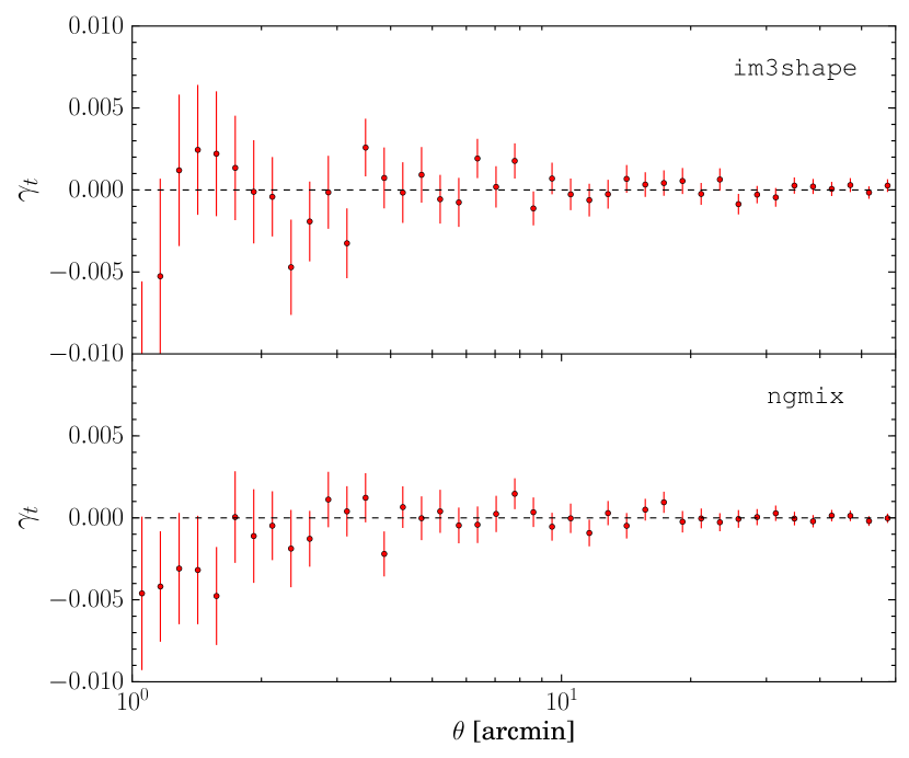
In Figure 17 we show the results of this test for both the im3shape and ngmix shear measurement pipelines. Uncertainties are jackknife estimates, made by splitting the total area into $152$ equal-area sub-fields. At large scales, the measurements are consistent with zero, but at scales less than about $10$ arcminutes there are a few consecutive bins with $\sim 1\sigma$ deviation from zero in both cases. The im3shape results show a slight oscillating pattern, and the ngmix results are slightly negative (a radial shear pattern).

None of these features is highly significant, especially since the points are somewhat correlated, so it may just be a noise fluctuation. Also, since the telescope distortion is largest at the edge of the field of view, we expected the absolute mis-estimation of the distortion to be largest at a separation of around $1$ degree. Furthermore, im3shape and ngmix use exactly the same WCS solution, since it is incorporated into the MEDS files directly. So the fact the tangential shear patterns are different in the two cases, and most significant near the centre, indicates that this is probably not due to errors in the WCS solution, although we do not have a good hypothesis for a plausible cause.

We estimated the magnitude of this potential additive systematic error in the same manner as we used above for the edge distortions. The mean spurious shear in this case has a magnitude of at most $0.005$ in both cases and occurs over a relative area of about $(2\arcmin/62\arcmin)^{2}=0.001$. The net additive systematic shear from this effect is thus at most $c_{\mathrm{rms}}=2\times 10^{-4}$, well below our requirements for an additive systematic shear.

We also looked at the shear around the CCD corners. While there was a very slight hint of a non- zero signal at small scales, the magnitude was even smaller than the shear around the field centres.

8.2 PSF Tests

If the PSF interpolation is not sufficiently accurate or if the shear algorithm does not fully account for the effects of the PSF convolution, the resulting shear estimates will include a spurious additive error that is correlated with properties of the PSF.

We looked for such additive errors by examining: (1) the mean shear binned by PSF ellipticity and PSF size, (2) the PSF-shear two-point correlation function and derived quantities, and (3) the tangential shear measured around stars.

8.2.1 PSF leakage

Figure 18: The mean galaxy shear as a function of the input PSF ellipticity ($e_{1}$ left, and $e_{2}$ right) for im3shape (top) and ngmix (bottom). The solid lines show the best linear fit without binning. Note the range of the abscissa is different for the ngmix and im3shape plots. The ngmix measurements are averaged over $r$, $i$, and $z$-band images, while the im3shape measurements use $r$-band images, and different models are used for measuring the ellipticity, resulting in different PSF ellipticity ranges for the two catalogues.

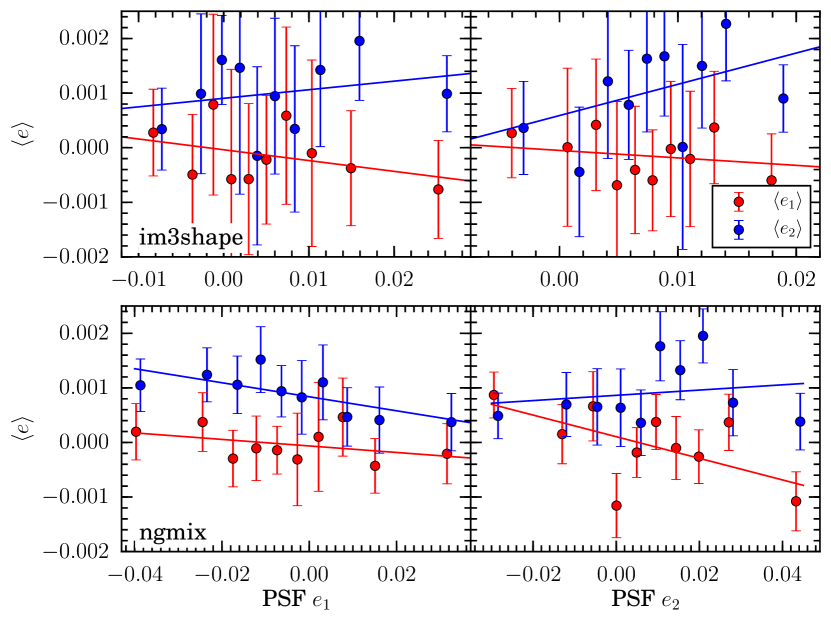
As we introduced in equation 3.4, we assumed that a component of the additive bias in the shear estimates comes from imperfect correction of the PSF, resulting in a term proportional to the PSF shape:

$$e_{\mathrm{gal}}=e_{\mathrm{true}}+\alpha e_{\textsc{psf}}+c.$$ (8.1)

A measured slope of galaxy ellipticity vs. PSF ellipticity can be identified as $\alpha$, where we use the mean PSF shape over all epochs.

The mean shear as a function of PSF ellipticity is shown in Figure 18 for both im3shape and ngmix galaxies. The points represent the mean galaxy ellipticity in each of 10 equal-number bins of PSF ellipticity. The line represents the best fit to the individual (unbinned) galaxy shapes. The slopes of the linear fits range from -2.0% to 5.7% $\pm$ 3% for im3shape and from -2.0% to 0.5% $\pm$ 1% for ngmix. The slopes are consistent with no PSF leakage for both catalogues.

To obtain a more precise estimate of $\alpha$, we computed the (weighted) average of the slopes of the red lines on the left plots (i.e. $\langle e_{1}\rangle$ vs. PSF $e_{1}$) and the blue lines on the right plots (i.e. $\langle e_{2}\rangle$ vs. PSF $e_{2}$). For im3shape we found $\alpha=0.008\pm 0.025$, and for ngmix $\alpha=-0.001\pm 0.007$. There is no evidence for non-zero $\alpha$; however, for im3shape, we cannot definitively confirm that $|\alpha|<0.03$ (cf. equation 3.15) given the uncertainty in the estimate.

Figure 19: The mean galaxy shear as a function of the input PSF size for im3shape (top) and ngmix (bottom). The solid lines show the best linear fit without binning.

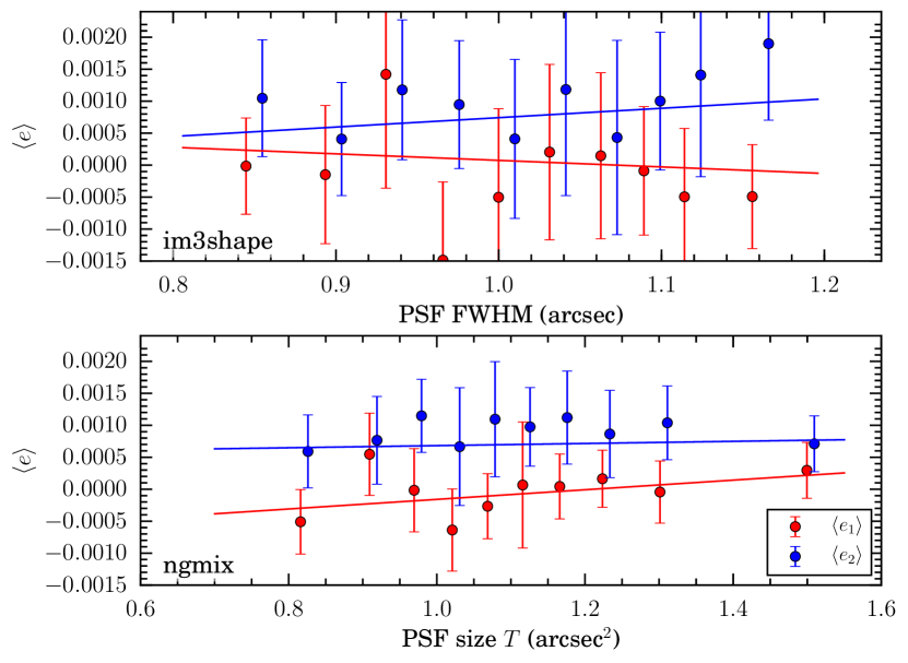
We similarly plot the mean shear as a function of PSF size in Figure 19 for both im3shape (left) and ngmix (right). Linear best-fitting lines are also included. The slopes here are also consistent with zero, being on the order of 0.1% or less, which indicates negligible dependence of the mean shear on the PSF size.

8.2.2 Star/galaxy cross-correlation

Another estimate of the leakage factor $\alpha$ comes from the cross-correlation of the galaxy shapes with the PSF shapes, $\xi_{+}^{gp}$. Writing $\xi_{+}^{gp}$ in terms of equation 8.1 and solving for $\alpha$, we find that

$$\alpha=\frac{\xi_{+}^{gp}-\langle e_{\mathrm{gal}}\rangle^{*}\langle e_{\textsc{psf}}\rangle}{\xi_{+}^{pp}-|\langle e_{\textsc{psf}}\rangle|^{2}},$$ (8.2)

where $\xi_{+}^{pp}$ is the auto-correlation function of the PSF shapes, $e_{\textsc{psf}}$.

While this nominally gives us an estimate of $\alpha$ as a function of scale, $\alpha$ is not a scale-dependent quantity. It is a quantification of a point process, the possible leakage of the PSF shape into the galaxy shape estimates. Therefore, we expect this estimate of $\alpha$ to be consistent at all scales, given the uncertainties in the estimate.

Figure 20: The calculation of the PSF leakage parameter $\alpha$, which is given in equation 8.2. The top plots show $\xi^{gp}$ (red), the cross correlation of the galaxy shapes with the PSF shapes, and $\xi^{pp}$ (blue), the auto-correlation of the PSF shapes, for im3shape (left) and ngmix (right). The bottom plots show $\alpha$, which is a measure of the leakage of the PSF shapes into the galaxy shapes as a function of scale. The grey band shows the sample variance plus shape noise uncertainty for $\alpha$. The $\chi^{2}/{\rm d.o.f.}$ is given for $\alpha$ over all scales.

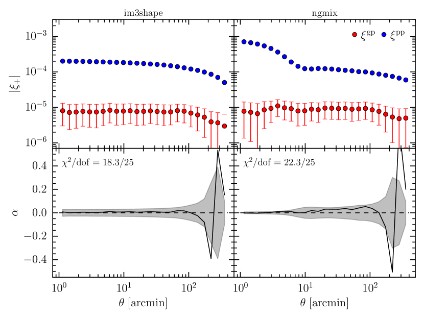
The measured $\xi_{+}^{gp}$ and $\xi_{+}^{pp}$ correlation functions are shown in the top panels of Figure 20 for im3shape (left) and ngmix (right). $\alpha$ is then calculated based on these and shown in the lower panels. Due to sample variance, $\alpha$ can be non-zero in this test even if the measured shears have no PSF contamination. We used the mock catalogues described in Becker et al. (2015) to compute the total uncertainty for $\alpha$. These catalogues were populated with PSF shapes by using the PSF shape from the nearest observed galaxy to each mock galaxy. We then used the full suite of 126 mock catalogues to compute the total uncertainty on $\alpha$ including both shape noise and sample variance.

We found that both im3shape and ngmix show no significant PSF contamination in this test, with a total $\chi^{2}/\mathrm{d.o.f.}$ of 18.3/25 and 22.3/25 for $\alpha$ computed over all scales. The best-fitting value for $\alpha$ in each case, properly taking into account the correlations (Avery, 1996), is $\alpha=0.010\pm 0.023$ for im3shape and $\alpha=-0.008\pm 0.006$ for ngmix, both below the requirement of $|\alpha|<0.03$ from equation 3.15, although in the case of im3shape we are only able to constrain $|\alpha|$ to be less than 0.03 at about $1\sigma$.

8.2.3 Tangential shear around stars

Figure 21: Tangential shear around stars for im3shape (blue) and ngmix (red). Stars are split into to two bins of $i$-band magnitude, where “bright” means $14<m_{i}<18.3$ and “faint” means $18.3<m_{i}<22$. The faint sample includes stars used for PSF modeling; bright stars are excluded to avoid the brighter-fatter effect (cf. §4.2). Shaded regions represent 1$\sigma$ shape noise uncertainty, while error bars are from jackknifing the stars.

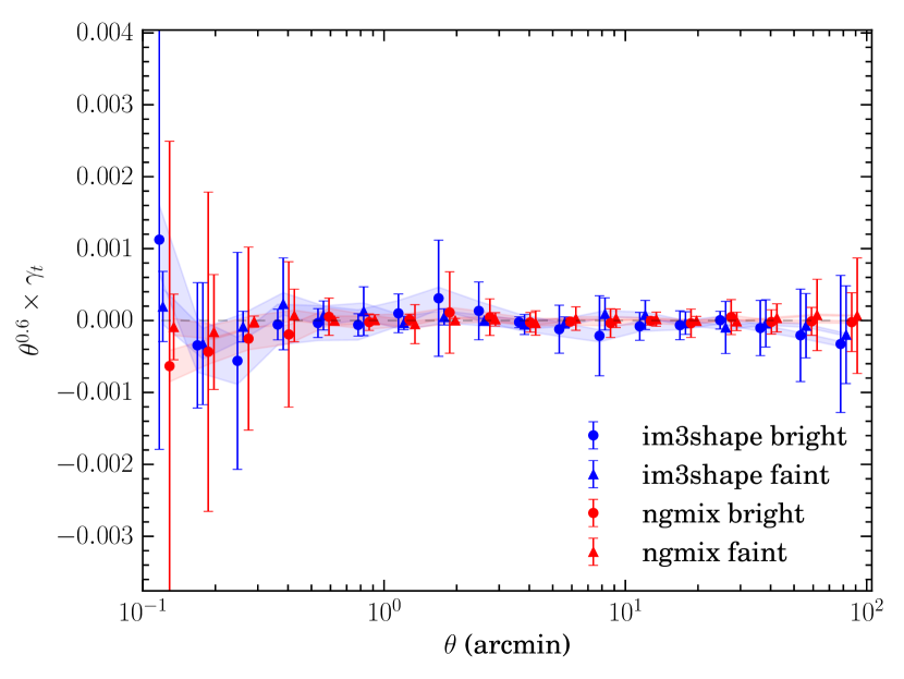
If the PSF correction is incomplete, there may also be a residual signal seen in the mean tangential shear around stars, which could potentially contaminate galaxy-galaxy lensing studies. To test for this, we measured the tangential shear around the positions of stars in both im3shape and ngmix for “bright” ($14<m_{i}<18.3$) and “faint” ($18.3<m_{i}<22$) stellar populations. In all cases we found the signal, shown in Figure 21, to be consistent with zero. The shape noise uncertainty is shown as the shaded regions. The error bars are jackknife uncertainty estimates.

The test using the faint stars primarily checks for effects related to PSF interpolation and PSF modeling. The bright stars are not themselves used to constrain the PSF model (cf. Figure 6), so these stars instead check for problems related to deblending and sky estimation errors in the outskirts of bright stellar haloes. We see no evidence of any systematic errors around either set of stars.

8.3 Galaxy Property Tests

There are many properties of the galaxy images that should be independent of the shear, but which in practice can be correlated with systematic errors in the shear measurement. For example, some of the properties we tested during the course of our analysis were: the size of the postage stamp, the number of neighbors being masked, the fraction of the stamp area being masked, the estimated bulge-to-disc ratio, the galaxy’s signal-to-noise, and the galaxy size. These were all extremely helpful diagnostic tools during the analysis, but here we only present the final two, which initially showed evidence of systematic errors and took the most effort to resolve.

Using $S/N$ or the galaxy size for selections is quite natural, since estimating the shear for small, faint galaxies is more challenging than for large, bright galaxies. However, measurements of these quantities can be correlated with the galaxy ellipticity, and thus an applied shear. Binning the data for the null test by these properties can thus induce selection effects and produce a net mean spurious ellipticity. This was already discussed in §7.2 with respect to $S/N$. We need to do something similar to construct a proper null test for the galaxy size.

8.3.1 Galaxy signal-to-noise

Figure 22: The mean galaxy shear as a function of the signal-to-noise for im3shape (top) and ngmix (bottom). For im3shape we test against $(S/N)_{w}$ (cf. equation 7.3), which is one of the parameters used for the calibration, so it includes corrections for selection bias. For ngmix, we test against $(S/N)_{r}$ (cf. equation 7.4), which does not induce any significant selection bias from the binning.

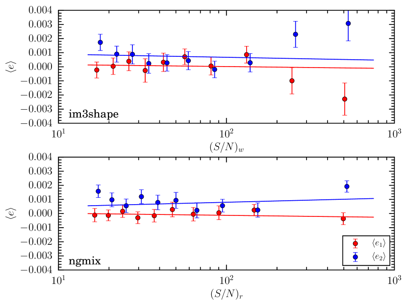
The null test for checking that the galaxy shapes are independent of $S/N$ requires different measures of $S/N$ for each catalogue. As described in §7.3.2, for im3shape we calibrated the bias in the shear measurements from simulations as a function of $(S/N)_{w}$ and $R_{gp}/R_{p}$. As such, the selection bias that is induced by binning on $(S/N)_{w}$ (cf. §7.2) is accounted for as part of the calibration. Thus, the appropriate null test on the data is to check that the mean shear is independent of $(S/N)_{w}$, as shown in the top panel of Figure 22. There is no apparent bias in the mean shear down to $(S/N)_{w}=15$.

We did not apply any external calibration to ngmix, so the null test for it requires a $S/N$ measure that does not induce selection biases from the binning. For ngmix, we used $(S/N)_{r}$ (cf. equation 7.4), which did not induce any selection biases when we tested it on simulated data. In the bottom panel of Figure 22 we show that the mean estimated shear for ngmix is independent of this “roundified” signal-to-noise measure down to $(S/N)_{r}=15$.

Previous versions of the ngmix catalogue had shown a very significant bias in the lowest $S/N$ bin in this plot before we realized that the bias was being induced by our galaxy selection from the cut on $(S/N)_{w}$. im3shape calibrates this kind of selection bias, but when that calibration is faulty, it too could show a bias in the lowest $S/N$ bin. In Figure 22 we show that the final catalogues do not have any such bias. The points are consistent with the mean value (which, as we mentioned, is not necessarily expected to be zero) and show maximal deviations less than our required $c_{\mathrm{rms}}<2\times 10^{-3}$ (equation 3.11).

8.3.2 Galaxy size

Similar considerations apply to the null tests for galaxy size. Since im3shape corrects for selection bias using the measured $R_{gp}/R_{p}$, this is the appropriate quantity to use for the null test regarding galaxy size. In the top panel of Figure 23 we show the mean estimated shear binned by $R_{gp}/R_{p}$. The im3shape measurements show no evidence of any dependence of the shear estimates on the size of the galaxy.

Figure 23: The mean galaxy shear as a function of the galaxy size for im3shape (top) and ngmix (bottom). For im3shape we test against $R_{gp}/R_{p}$, which is one of the parameters used for the calibration, so it includes corrections for selection bias. For ngmix, we test against a size measure, $T_{r}$ (cf. equation 8.4), that does not induce and significant selection bias from the binning.

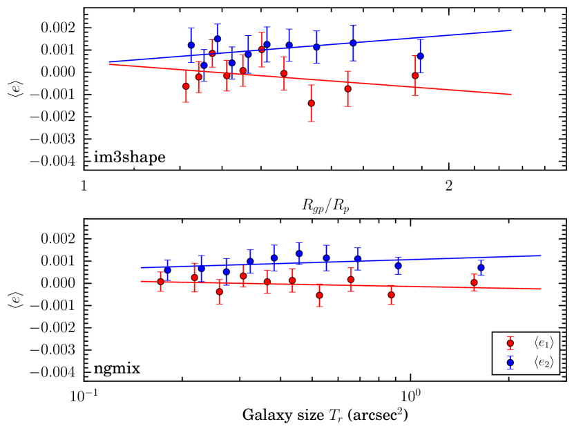
For ngmix, we need to use a size measure that is independent of the shape of the galaxy. The internal parameter that ngmix uses for the size of the galaxy in its model is $T=I_{xx}+I_{yy}$, the standard second moment measure of the size of a galaxy; however, this quantity changes with applied shear. If a round galaxy is sheared by an area-preserving shear $g$, then the measured size will be

$$T^{(g)}=T^{(g=0)}\left(\frac{1+|g|^{2}}{1-|g|^{2}}\right).$$ (8.3)

For non-round galaxies, an applied shear tends to make the estimated size $T$ larger when the shear is aligned with the galaxy shape and smaller when it is anti-aligned. This can lead to an apparent bias in the measured shapes with respect to the measured value of $T$. If the mean PSF shape were precisely round, this bias should average out over an ensemble of galaxies; however, our PSFs have a preferred direction, which breaks the symmetry and leads to an apparent bias in the mean shape with respect to $T$.

In parallel to our definition of $(S/N)_{r}$ as the signal-to-noise that the galaxy would have had if it were round, we similarly construct an estimate of the size that the galaxy would have had if it were round:

$$T_{r}\equiv T\left(\frac{1-|e|^{2}}{1+|e|^{2}}\right),$$ (8.4)

where $e$ is the estimated shape of the galaxy. Binning the shears by this quantity should thus not induce any selection bias from the binning itself. In the lower panel of Figure 23 we show the results of this test for ngmix. There is no apparent dependence of the mean shape on this “roundified” measure of the size of the galaxy.

In both cases the slopes are consistent with zero and show maximal deviations well below our required $c_{\mathrm{rms}}<2\times 10^{-3}$ (equation 3.11).

8.4 B-mode Statistics

The deflection field induced by gravitational lensing has the special property that it is essentially curl-free. Since this is also true of electric fields, the shear field is generally referred to as being an “E-mode” field. The corresponding divergence-free “B-mode” field can be considered as corresponding to an imaginary convergence (Schneider et al., 2002).

In fact gravity can induce a slight B-mode from source clustering (Schneider et al., 2002), multiple deflections (Krause & Hirata, 2010), and intrinsic alignments (Crittenden et al., 2001). But in practice all of these effects are well below the level at which we could measure them, which means that any significant measured B-mode is almost certainly a sign of uncorrected systematic errors in the shears.

We calculated B-mode statistics of the shear field by computing linear combinations of the binned shear two-point correlation function values that are insensitive to any E-mode signals, modulo a very small amount of computable E- to B-mode leakage. See Becker (2013) for details. In this application, we chose linear combinations that approximate band-powers in Fourier space as described in Becker & Rozo (2014). Finally, we used the mock catalogues described in Becker et al. (2015) to compute the shape noise and sample variance uncertainty for the statistics. These mock catalogues include the survey mask and match the shape noise and source photometric redshift distribution for each of the two shear catalogues. We used 126 mock catalogues in total.

Figure 24: The measured B-mode for ngmix (top) and im3shape (bottom). Each band power measurement is plotted at its central location in $\ell$. The grey band shows the uncertainty on the measurement due to both sample variance and shape noise. Adjacent points are highly correlated and the indicated $\chi^{2}$ accounts for the correlations.

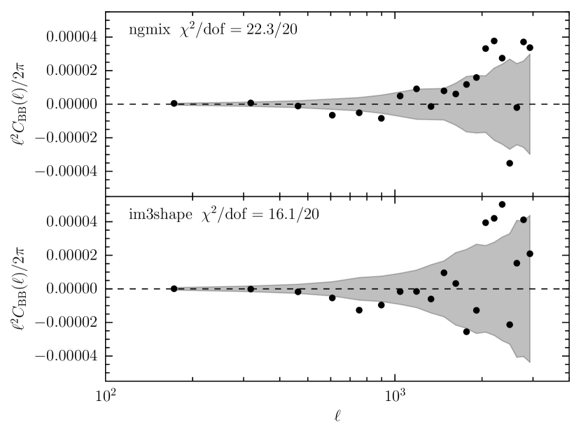
In Figure 24 we show the measured B-mode for each catalogue using the most conservative selection described below. Each band-power measurement is plotted at its central location in $\ell$. Adjacent points are highly correlated and the $\chi^{2}$ given in the figure accounts for the correlation. We find a $\chi^{2}/\mathrm{d.o.f.}$ of 22.3/20 for ngmix and 16.1/20 for im3shape indicating no significant B-mode contamination in the shear field.

8.5 Calibration Tests

It is difficult to test the overall shear calibration using the data alone. However, we can use the GREAT-DES simulation described in §6.1 to test the performance of the two shear algorithms on relatively realistic images with known applied shear.

Since im3shape uses this simulation to calibrate the shear measurements (cf. §7.3.2), the overall corrected shears should be accurate, almost by construction. The calibration was done without weighting, but for this test we used the same weights that we recommend for the data (cf. §7.3.4). The mean shear is thus not mathematically guaranteed to be exactly zero. We detect a net bias after applying the calibrations, but it less than our requirements for DES SV data: $m_{1}=0.0008\pm 0.0015$ and $m_{2}=-0.0068\pm 0.0015$.

For ngmix, the overall calibration error is a more relevant test. The priors used for GREAT-DES were the same as used for the DES SV data, which is expected to be appropriate given the general agreement between the galaxy properties in the simulation and the data (cf. §6.1). We found the overall calibration error for ngmix to be $m_{1}=-0.030\pm 0.0015$ and $m_{2}=-0.035\pm 0.0015$. This does not quite meet our requirement of $|m|<0.03$ from equation 3.10.

Considering that many science applications will use tomography to investigate the evolution of the shear signal with redshift, it is interesting to look at the calibration of both shear codes as a function of redshift. To test the redshift dependence of the bias, we used the known photometric redshifts of the galaxies from the COSMOS data, from which we drew the galaxy images used in the GREAT-DES simulation. With this test, we can also learn if the tomographic selection process itself leads to any significant selection biases.

In Figure 25 we show the results of performing this test for ngmix (top) and im3shape (bottom), taking galaxies in different ranges of photometric redshift, using the same redshift bins that will be used for the cosmology constraints (The Dark Energy Survey Collaboration et al., 2015). Note that the redshift information was not used in the calibration process for im3shape, so the variation with redshift is a non-trivial test of the correction. Prior to calibration, we find a significant bias in each of the three redshift bins, $m=(-0.039,-0.058,-0.072)$. After calibration (red circles, Figure 25), the net multiplicative bias for im3shape is reduced to a level well within the requirements. This indicates that the derived corrections are robust to galaxy selections based on redshift.

Figure 25: Multiplicative shear bias in three bins of photometric redshift for ngmix (top) and im3shape (bottom), as calculated using the GREAT-DES simulation. In both cases, the same selection and weights were used as for the real data. The red circles denote the average bias in each bin after correcting for the sensitivity (ngmix) or the calibration (im3shape). The blue triangles show an estimate of selection bias, calculated using the known true ellipticities. The grey band in both panels marks the $\pm$3% requirement for SV data.

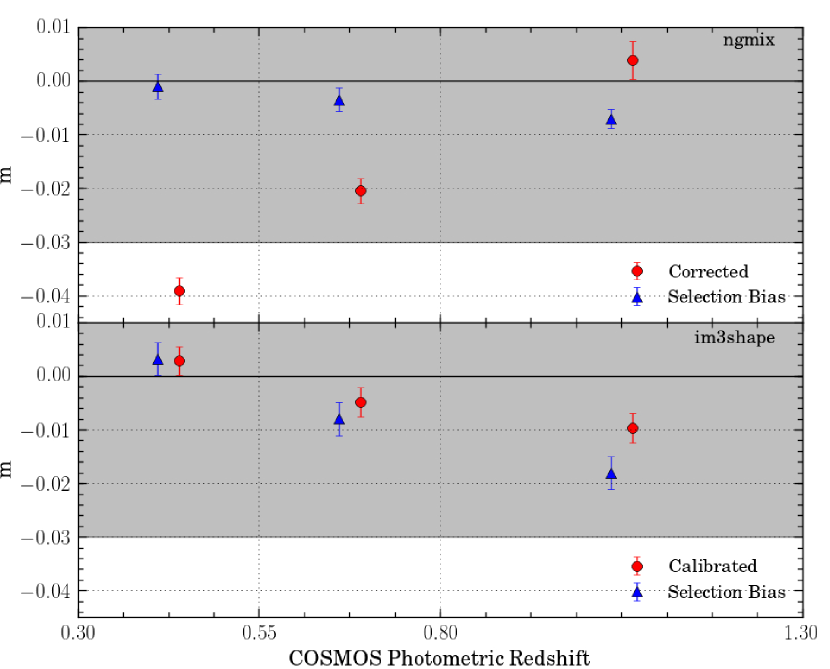
We also tested the performance of im3shape’s PSF leakage calibration as a function of redshift (not shown). We found the overall leakage before calibration was $\alpha=(0.070,0.112,0.102)$ for the three redshift bins. After calibration, we found $\alpha=(0.001,0.021,-0.005)$, which demonstrates good performance of the leakage calibration as well.

We found the multiplicative bias for ngmix to be outside of the requirement band for the lowest redshift bin, and then rose to acceptable levels in the two higher bins. We believe this is because the proportion of bulge galaxies is highest at low redshift, and the ngmix exponential model has significant model bias for these galaxies. As the proportion of bulges decreases at higher redshift, the mean model bias decreases, and the calibration is within our requirements.

To test the hypothesis that we are measuring a model bias for the exponential disc model, we implemented a more flexible model and applied it to this simulation. This model is a simple two-component bulge and disc model, where the bulge fraction is determined not by a simultaneous fit with other parameters but by an initial comparison of two separate bulge and disc fits to the galaxy image. A similar model used in the Sloan Digital Sky Survey for galaxy fluxes was known as the “composite” model (Abazajian et al., 2004). For the composite model we found biases $\sim 1$%, suggesting that the larger bias evident for the exponential model is principally model bias. Unfortunately, we were unable to apply this new composite model to the DES data in time to be used for this paper.

The blue triangles in Figure 25 represent the estimated selection bias in each bin induced by our various selection criteria. To calculate these values, we applied the known shear to the COSMOS shape estimates (Kannawadi et al., 2015) of the galaxies used for the simulation, and then applied the same selection criteria we used for each of the two algorithms. We found the selection bias from the im3shape cuts was at most $2\%$ in the highest redshift bin, which is largely corrected by the calibration scheme. We found the selection bias for ngmix was less than $1\%$ for all redshift bins.

8.6 Cross-catalogue Comparisons

Another powerful test is to compare the two independent shear catalogues, im3shape and ngmix. We used two very different strategies when generating these catalogues. For im3shape we used simulations to determine the shear calibration, and applied corrections to the shear measurements on real data. For ngmix we expected relatively little noise bias, but the sensitivity of the shear estimator was calculated from the data itself and applied to the shear measurements, a process that was worth testing in detail. And we did expect some model bias for ngmix. Furthermore, the PSF was treated differently by the two methods: for im3shape we used the reconstructed PSF image directly, and for ngmix we fit models to the PSF.

A direct galaxy-by-galaxy test is not appropriate for a cross-catalogue comparison, since there is not a unique unbiased shear estimate for a single galaxy. Rather, we wished to test that both methods produced consistent shear statistics for an ensemble of galaxies (cf. Velander et al., 2011). Two potential shear statistics that can be used are a galaxy-galaxy lensing signal and the two-point shear correlation function. We tested if the results were consistent when using the same ensemble of galaxies with the same weighting.

Disagreement between the catalogues would be proof that at least one catalogue is biased, but we would not be able to determine which one, nor the magnitude of this bias. Agreement between the two catalogues is subjectively reassuring, but we wish to emphasize that agreement does not prove that both catalogues are “correct” in the sense that they can be used to generate unbiased shear estimates.

8.6.1 Tangential shear ratio

Galaxy-galaxy lensing provides one of the cleanest tests of the relative calibration of the two catalogues, because the azimuthal symmetry inherent in the tangential shear signal largely cancels most sources of additive systematic error. Thus the ratio of two tangential shear signals is primarily a measure of the relative multiplicative errors between the two catalogues.

For this test, we used the tangential shear signal around Luminous Red Galaxies (LRGs) as determined by redMaGiC (red sequence Matched-filter Galaxies Catalogue; Rozo et al., 2015) from the same DES SPT-E data. For this purpose, we did not require sources to be behind the lenses. Rather, we took the full LRG catalogue as the lenses, and for the sources, we used all galaxies that were well-measured by both ngmix and im3shape. Regardless of the redshifts of the LRGs and the source galaxies, we expected the signal to be the same for both catalogues in the absence of a multiplicative bias.

The observed signal $\langle e_{t,i}(\theta)\rangle$ for each method $i\in$ {im3shape, ngmix} can be written as:

$$\langle e_{t,i}(\theta)\rangle=(1+m_{i})\langle\gamma_{t}(\theta)\rangle+\langle\eta_{i}(\theta)\rangle,$$ (8.5)

where $\langle\gamma_{t}\rangle$ is the true underlying signal, $\langle\eta_{i}\rangle$ is a noise term including both intrinsic shape noise and measurement noise, and $m_{i}$ is a possible calibration error for each method. We mostly drop the argument $\theta$ in the following for brevity. For the same ensemble of galaxies, the two catalogues have identical values of $\langle\gamma_{t}\rangle$ and a similar shape noise contribution to $\langle\eta_{i}\rangle$ (though not identical, since the two methods use different bands). The contribution to $\langle\eta_{i}\rangle$ from shape measurement noise, however, is expected to be somewhat different.

Figure 26: The ratios of tangential shear measurements around LRG galaxies from shears measured by ngmix to those measured by im3shape. The red circles show the direct ratio and the triangles correspond to the ratio after subtraction of the tangential shear around random points. The weighted mean ratio in the scale range $1-20$ arcminutes is $0.954\pm 0.018$. The blue line shows a prediction of the ratio ($0.94$) based on the GREAT-DES simulation, which accounts for a selection bias induced by the intersection of the two shape catalogues. This result is in good agreement with the data points.

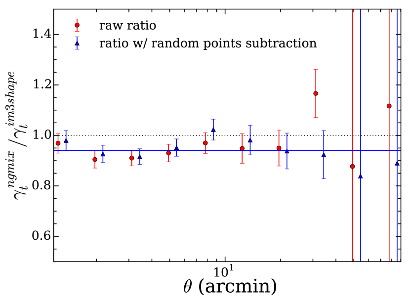
The red points in Figure 26 represent the ratio of measured tangential shear using the two shear catalogues. The weighted mean of the ratio over the range from 1 to 20 arcminutes (the typical scales of interest for weak lensing) is $0.932\pm 0.018$. We would naively expect this to be an estimate of $(1+m_{\textsc{ngmix}})/(1+m_{{\textsc{im3shape}}})\approx 1+m_{\textsc{ngmix}}-m_{{\textsc{im3shape}}}$. However, three corrections are required before any conclusions can be drawn from this result about potential differences in the relative calibration.

First, additive systematic errors only cancel if the sources are distributed uniformly around the lenses. This is approximately true, but masking can break the symmetry, especially at large scales. One solution is to subtract off the measured tangential shear around random points, drawn from the same region and with the same masking as the LRGs. No signal is expected around such points, but any additive bias will affect both measurements equally. Thus the difference is a cleaner estimate of the true tangential shear than the uncorrected signal. The blue points in Figure 26 represent the signal after this subtraction, and have a mean ratio of $0.954\pm 0.018$,

Second, the ratio of two noisy quantities with the same mean does not in general have an expectation value equal to 1. If the denominator is a random variable, $X$, with a symmetric probability distribution (e.g. $X\sim\mathcal{N}(\bar{X},\sigma_{X})$), the ratio will be approximately $1+\sigma_{X}^{2}/\bar{X}^{2}$. To account for this bias, we created simulated realizations of the ratio, and compared the measured signal to the mean and variance of these. We generated a ratio realization in the following way:

1. Fit a polynomial, $\log(\langle e_{t}\rangle(\theta))\!=\!p(\log(\theta))$ to the measured ngmix signal, and take this to be the true signal, $\hat{\gamma}_{t}(\theta)$.

2. For each source in the ensemble, rotate both the ngmix and im3shape shear by the same random angle.

3. Re-measure the two tangential shear signals, which now give estimates of the noise, $\langle\eta^{r}(\theta)\rangle$, as the true signal is removed by the random rotations.

4. Compute the realization ratio as

   $$(\hat{\gamma}_{t}+\langle\eta_{\textsc{ngmix}}^{r}\rangle)/(\hat{\gamma}_{t}+\langle\eta_{{\textsc{im3shape}}}^{r}\rangle).$$ (8.6)

We found the mean of these realizations to be consistent with a ratio of 1 on all scales, which means that the $S/N$of the tangential shear is high enough that we can neglect the noise term in the denominator.

Finally, we found that the act of matching the two catalogues caused a selection bias in the ngmix catalogue, for two reasons. First, the im3shape algorithm failed more often for objects with low Sérsic index ($n<1$). And second, the cuts we made on the im3shape measurements of $(S/N)_{w}$ and $R_{gp}/R_{p}$ altered the mix of galaxy properties in the matched catalogue. These two selection effects, when applied to the ngmix catalogue imparted a net bias on the ngmix shear estimates in the matched catalogue that was not present in the full ngmix catalogue.

Figure 27: Multiplicative bias for ngmix shear measurements on GREAT-DES simulated data as a function of redshift. The red circles show the bias calculated using all galaxies that pass the ngmix selection criteria (as in the upper panel of in Figure 25). The blue triangles show the bias when also including the recommended im3shape selection, as we do to obtain the matched catalogue used for Figure 26. As in Figure 25, the grey band represents the $\pm$3% requirement for the SV data.

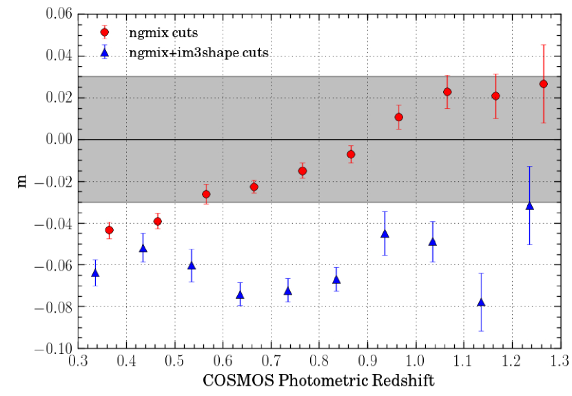
We quantified the level of this selection bias by performing the same procedure on the GREAT-DES simulation. We compared the mean bias for ngmix using the canonical ngmix selection criteria to the bias after applying the im3shape selection, as a function of redshift. The result is shown in Figure 27. The matching induced a mean selection bias of about $-3\%$. Furthermore, we found that this bias increased with redshift. Weighting the bias according to the lens redshift distribution and the lensing efficiency of the source galaxies used in the tangential shear ratio test (and assuming that the lenses do not evolve with redshift), we found a net selection bias of $-6\%$ for ngmix in the matched catalogue relative to whatever bias might be present in the full ngmix catalogue.

The mean ratio of $0.954\pm 0.018$ is thus consistent with the prediction from GREAT-DES of $-6\%$ selection bias (which would produce a ratio of $0.94$). This bias induced by the combination of im3shape and ngmix selection criteria in the matched shape catalogues is shown by the blue line in Figure 26. Our finding is therefore consistent with no relative multiplicative bias between the two catalogues.

We cannot of course prove that neither catalogue is affected by a significant multiplicative bias based on this test. They could both be biased by the same amount in either direction. Furthermore, there are significant uncertainties in the calculation of the predicted selection bias described above that may be at the $\sim 3\%$ level.

8.6.2 Differential shear correlations

The two-point shear correlation function is much more sensitive to additive shear errors than the tangential shear, as mentioned above; it would be difficult to disentangle multiplicative and additive errors in a ratio test. Even in the absence of additive errors, the ratio of shear correlation functions is much noisier than the ratio of tangential shears, making it a less stringent test of calibration.

For these reasons, we instead use the two point function of the difference in the shear estimates from ngmix and im3shape to compare the shear catalogues:

$$\xi_{+,\Delta e}(\theta) =\langle(e_{\textsc{ngmix}}(\mathbf{x})-e_{{\textsc{im3shape}}}(\mathbf{x}))^{*}$$

$$\qquad(e_{\textsc{ngmix}}(\mathbf{x}+\boldsymbol{\theta})-e_{{\textsc{im3shape}}}(\mathbf{x}+\boldsymbol{\theta}))\rangle.$$ (8.7)

Consider the following model for the additive systematic errors in each catalogue (labelled $i$ here):

$$e_{i}=(1+m_{i})\gamma+\eta_{i}+a_{i}c_{\rm common}+c_{i},$$ (8.8)

where $m_{i}$ is the calibration error, $\eta_{i}$ is the noise in the estimate, $c_{\rm common}$ includes any additive systematic errors present in both catalogues, possibly multiplied by different coefficients $a_{i}$, and $c_{i}$ is the additive error particular to each catalogue.

By construction, the additive bias terms in equation 8.8 are independent. If we further make the assumption that the systematic errors are uncorrelated with the applied shear and the noise, and that $m$ and $c$ are uncorrelated, we find that

$$\xi_{+,\Delta e}(\theta) =(\Delta m)^{2}\xi_{+}(\theta)$$

$$\quad+(\Delta a)^{2}\langle c_{\rm common}^{*}c_{\rm common}\rangle(\theta)$$

$$\quad+\langle c_{\textsc{ngmix}}^{*}c_{\textsc{ngmix}}\rangle(\theta)$$

$$\quad+\langle c_{\textsc{im3shape}}^{*}c_{\textsc{im3shape}}\ \rangle(\theta).$$ (8.9)

This test is sensitive to the spatial correlations of the systematic errors in either catalogue, but particularly to additive errors, rather than multiplicative. The $(\Delta m)^{2}$ factor for the multiplicative term typically makes this term insignificant.

There is one subtlety in the construction of this test. As we found in §8.6.1, the act of matching the two catalogues can induce selection biases that are not present in either catalogue separately when using its own individual selection criteria. In this case, the salient selection effects are a spurious PSF leakage $\alpha$ and an overall mean $\langle c\rangle$ that can be induced by the match.

The estimated value of $\alpha$ for ngmix changed by less than $0.1\%$ in the matched catalogue relative to the full ngmix catalogue. But for im3shape, the matching changed $\alpha$ by $-1.5\%$. Therefore, to make this a fair test of the additive systematic errors, we added back $0.015\times e_{\textsc{psf}}$ to the im3shape galaxy shapes to account for this selection effect.

Even after correcting for the above effect, we found that the mean shear changed by $(3.9+2.2i)\times 10^{-4}$ for ngmix and by $(2.0-3.0i)\times 10^{-4}$ for im3shape. We interpreted these changes as due to selection biases from the matching itself, leading to a spurious overall $\langle c\rangle$ for each catalogue. We thus subtracted these values as well from the shape estimates in each catalogue.

Figure 28: The shear auto-correlation function of the difference in shear estimates of ngmix and im3shape. This test shows the level of additive systematic errors that may still be present in one catalogue that is not present in the other. The yellow band is the requirement, $\delta\xi^{\mathrm{max}}_{+}$ from Figure 3.

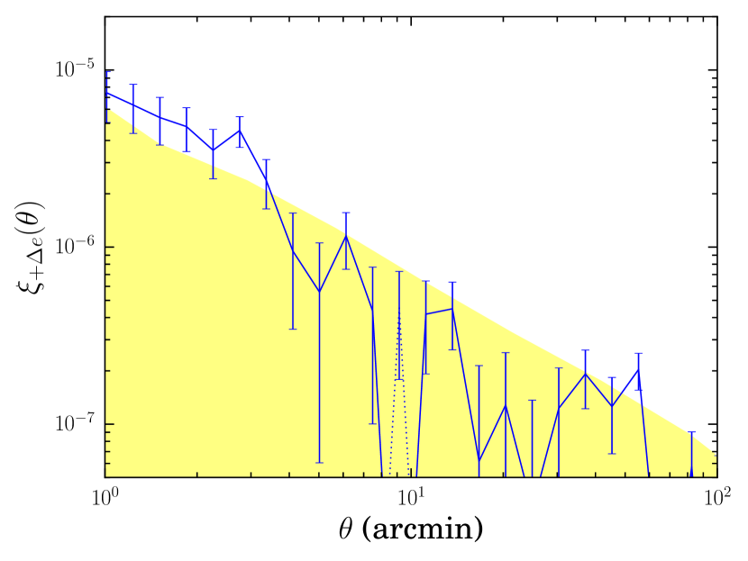
Test	Upper Limit on Systematic Error
	im3shape	ngmix
PSF Model Tests
§4.2 Mean PSF size error	$|m|<0.005$	$|m|<0.01$
§4.4 PSF model diagnostics $\rho_{1,3,4}$	$\xi_{+}^{cc}(1\arcmin)<$ $2\times 10^{-6}$$\dagger$	$\xi_{+}^{cc}(1\arcmin)<5\times 10^{-6}$
	$\xi_{+}^{cc}(30\arcmin)<$ $7\times 10^{-8}$	$\xi_{+}^{cc}(30\arcmin)<9\times 10^{-8}$
§4.4 PSF model diagnostics $\rho_{2,5}$	$\xi_{+}^{cc}(1\arcmin)<$ $2\times 10^{-7}$	$\xi_{+}^{cc}(1\arcmin)<8\times 10^{-8}$
	$\xi_{+}^{cc}(30\arcmin)<$ $1.5\times 10^{-7}$	$\xi_{+}^{cc}(30\arcmin)<1.4\times 10^{-7}$
Spatial Tests
§8.1.1 Position in the field of view	No evidence of systematic errors	No evidence of systematic errors
§8.1.2 Position on CCD	$\xi_{+}^{cc}(1\arcmin)<6\times 10^{-7}$	$\xi_{+}^{cc}(1\arcmin)<6\times 10^{-7}$
§8.1.3 Tangential shear around field centres	$\xi_{+}^{cc}(1\arcmin)<4\times 10^{-8}$	$\xi_{+}^{cc}(1\arcmin)<4\times 10^{-8}$
PSF Tests
§8.2.1 PSF leakage	$|\alpha|<0.04$	$|\alpha|<0.01$
§8.2.1 Dependence on PSF size	No evidence of systematic errors	No evidence of systematic errors
§8.2.2 Star-galaxy cross correlation	$|\alpha|<0.03$	$|\alpha|<0.015$
§8.2.3 Tangential shear around stars	No evidence of systematic errors	No evidence of systematic errors
Galaxy Property Tests
§8.3.1 Galaxy $S/N$	No evidence of systematic errors	No evidence of systematic errors
§8.3.2 Galaxy size	No evidence of systematic errors	No evidence of systematic errors
B-mode Statistics
§8.4 $\ell^{2}C_{\mathrm{BB}}(\ell)/2\pi$	No evidence of B-mode	No evidence of B-mode
Calibration Tests
§8.5 Redshift dependence in GREAT-DES	$|m|<0.02$	$|m|<0.04$
Cross-catalogue Comparison
§8.6.1 Tangential shear ratio	$|\Delta m|\lesssim 0.04$
§8.6.2 Differential shear correlations	$|\xi_{+}^{cc}(1\arcmin)|<9\times 10^{-6}$
	$|\xi_{+}^{cc}(30\arcmin)|<$ $2\times 10^{-7}$

^$\dagger$ Since im3shape use only the $r$-band images, the values quoted here are based on the $\rho$ statistics measured for the $r$-band-only PSFs. These curves are a bit higher than what is shown in Figure 10, which uses $r,i,z$ bands.

Table 2: Summary of the results of our suite of null tests (including tests in §4.4). For reference, our nominal requirements from §3 are $|\alpha|<0.03$, $|m|<0.03$, $\xi_{+}^{cc}(1\arcmin)<7\times 10^{-6}$, and $\xi_{+}^{cc}(30\arcmin)<2.5\times 10^{-7}$.

In Figure 28 we show the resulting correlation function (equation 8.7) after subtracting these selection biases. For the weights, we used $w=\sqrt{w_{\textsc{ngmix}}\times w_{\textsc{im3shape}}}$. The yellow band represents our requirement for additive systematic errors from equation 3.12. We see that, at scales less than 3 arcminutes, we do not quite meet the requirements. Either one or both catalogues apparently have non-negligible additive systematic errors at these scales. We recommend that science applications sensitive to additive systematic errors check carefully how these small-scale systematic errors may affect their science results.

8.7 Summary of Systematics Tests

We now attempt to synthesize the results of our large suite of null tests. With this many tests, even if all the tests pass individually, it would not necessarily imply that the total systematic error is below our requirements. In this section we attempt to quantify an upper limit on the level of systematic error that may be in the shear catalogues, given all of the information we have available.

In Table 2 we provide a summary of the results from the previous sections (including the tests in §4). For each, we have converted the result of the test into the impact that the result could have on 4 possible values. For PSF leakage, we give the maximum allowed value of $\alpha$. For other kinds of additive systematic errors, we give the maximum value of $\xi_{+}^{cc}(\theta)$ at $\theta=1$ arcminute and (when relevant) $30$ arcminutes. And for multiplicative errors, we give the maximum $|m|$ that is consistent with the test. Some tests do not lend themselves to a quantitative upper limit. Fortunately, in each of these cases, there is no evidence from the test that there is any systematic error.

There are two tests that give constraints on the PSF leakage coefficient $\alpha$. In all cases, the tests are completely consistent with $\alpha=0$. However, given the uncertainties in each case, we think it is appropriate to take the upper limit from the star-galaxy correlation function estimate, since it is the more precise estimate in both cases. This gives us limits of $\alpha<0.03$ for im3shape and $\alpha<0.015$ for ngmix. We can multiply this by $\xi_{+}^{pp}$ to give a limit on the maximum additive systematic error we may have at $1\arcmin$ and $30\arcmin$ due to PSF leakage.

For the other additive systematic errors, we can add them together linearly. $\xi$ acts like a variance, so systematic uncertainties add linearly, not in quadrature. However, the differential shear correlation test is different from the others. It includes many of the additive systematic errors tested by other tests, and in particular would almost certainly incorporate any systematic error due to PSF leakage, as the mechanism for any such leakage would be different for the two algorithms. Thus, it actually places a tighter limit on the potential systematic error from PSF leakage at $30\arcmin$ than the direct estimate of $\alpha$.

The differential shear correlation does not however include all of the additive errors from the PSF model tests. The two codes use the same PSF model for the $r$-band exposures, although ngmix also uses $i$ and $z$-bands. We conservatively assume that the PSF modeling systematic errors act as $c_{\mathrm{common}}$ terms in the nomenclature of §8.6.2 and add them to the estimate from the differential shear correlation to get our final estimate on the possible additive systematic error in each catalogue:

im3shape $$\begin{array}[]{l}\left|\xi_{+}^{\mathrm{sys}}(1\arcmin)\right|<1.1\times 10^{-5}\\ \left|\xi_{+}^{\mathrm{sys}}(30\arcmin)\right|<4\times 10^{-7}\end{array}$$ (8.12)

ngmix $$\begin{array}[]{l}\left|\xi_{+}^{\mathrm{sys}}(1\arcmin)\right|<1.4\times 10^{-5}\\ \left|\xi_{+}^{\mathrm{sys}}(30\arcmin)\right|<4\times 10^{-7}.\end{array}$$ (8.15)

Note that we are not claiming that either catalogue has systematic errors as large as this. Rather, we are claiming at $\sim 1\sigma$ level of confidence that the additive systematic errors in the two catalogues are smaller than this.

The limits on the multiplicative systematic errors come from two sources. We have estimated the bias on simulated data, and we have measured the relative bias of the two catalogues with respect to each other. With the exception of the lowest redshift bin for ngmix, where we found a bias of $m\simeq-0.04$, all of the tests are consistent with $|m|<0.02$ for both catalogues.

Investigation of the low redshift result for ngmix indicates that it is largely due to that bin having more bulge galaxies than the higher-redshift bins, leading to increased model bias there. However, Figure 12 shows that the distribution of bulges in GREAT-DES may not match the data very well, in particular as a function of $S/N$, which is correlated with redshift. This makes us uncertain how applicable the $m\!=\!-0.04$ result is to the SV data.

Furthermore, while the tangential shear ratio test showed that the two catalogues were consistent to within $|\Delta m|\!<\!0.02$, this was only after correcting for a matching-induced selection effect of $\Delta m\!\simeq\!0.06$. This correction involves a number of assumptions, so we are not confident that it is more precise than about $\pm 0.03$.

For these reasons, we feel that an appropriate upper limit on $m$ for both catalogues is

$$|m|<0.05.$$ (8.16)

We recommend science applications that are sensitive to multiplicative bias marginalize over a Bayesian prior on $m$ centred at $0$ with a standard deviation of $0.05$.

9 Shear Catalogues

The final shear catalogues are publicly available on the DESDM Releases web page. See that web page for complete documentation about how to access these catalogues, as well as the other DES SV catalogues that are available.

In this section we describe the final galaxy selection, how to correctly apply the calibrations and sensitivities to ensembles of galaxies, and what final number density we achieve. Appendix B has further details about the content and structure of the catalogues.

9.1 Final Galaxy Selection

The starting point for our galaxy catalogues was described in §2.1 and §2.2. The former described how we selected regions of the survey where we trust the images, and the latter described our initial galaxy selection function. We now describe further cuts informed by the suite of null tests in §8, such that the final shear catalogues were found to pass our tests.

We removed individual objects according to the following criteria:

• SExtractor flags = 1 or 2. Objects with higher SExtractor flags were already been removed from the input catalogues, since they are clearly problematic for a shape measurement code. But these two flags indicate that the object is likely to be blended, and thus the shape measurement was likely to be corrupted.

• “Crazy colours”. Individual objects with questionable colours are probably contaminated by cosmic rays or other defects, so their shapes are also likely to be inaccurate.

• Very low surface brightness. We found a class of spurious objects with very large sizes, but relatively low flux that were usually associated with various image artefacts. We excluded objects with $i+3.5\log(f_{i}/T)<28$, where $f_{i}$ is the $i$-band flux, and $T=I_{xx}+I_{yy}$ is the (deconvolved) object size estimated by ngmix. This cut is efficient at bright fluxes, but less so at faint fluxes, removing a significant number of real galaxies.

• Tiny size. If the ngmix estimate of the object size is very small, then the object is probably a star. Specifically, we removed objects with $T+\sigma_{T}<0.02$ square arcseconds.

From the resulting set of “good galaxies”, we then made a further selection based on both $S/N$ and the size of the galaxy relative to the PSF size, such that the resulting ensembles of shear estimates passed the null tests.

As we have already mentioned in §7.3.2, the im3shape selection needs to be made using $(S/N)_{w}$ and $R_{gp}/R_{p}$, since these are the parameters used for the shear calibration. ngmix does not do any calibration, so its selection is made using $(S/N)_{r}$ and $T_{r}/T_{\textsc{psf}}$ (cf. equations 7.4 & 8.4) to avoid inducing a selection bias.

The selection that we find passes the suite of null tests is the following:

$${\textsc{im3shape}}:\quad \begin{array}[]{l}(S/N)_{w}>15\\ R_{gp}/R_{p}>1.2\end{array}$$

$$\textsc{ngmix}:\quad \begin{array}[]{l}(S/N)_{r}>15\\ T_{r}/T_{\textsc{psf}}>0.15.\end{array}$$

We used this selection for all of the test results shown in §8.

Figure 29: A histogram of the $r$-band magnitude distribution showing the application of the various selection criteria from the initial “Gold” Catalogue to the two final shear catalogues. The dark red and blue show the galaxies with sufficiently accurate shape for ngmix and im3shape respectively.

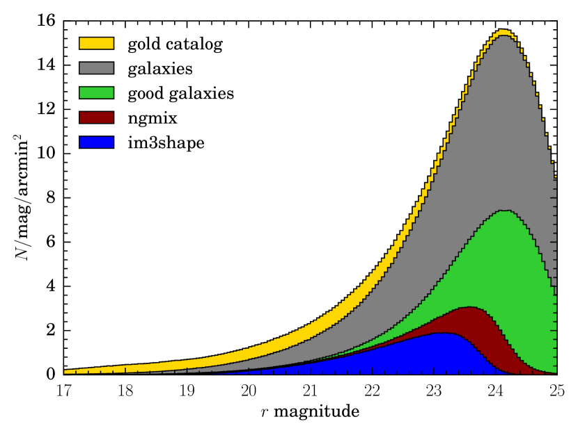
In Figure 29 we show the effect that successively applying each round of selections has on the distribution of $r$-band magnitudes, starting with the original Gold Catalogue, selecting possible galaxies, removing problematic galaxies, and then applying the $S/N$ and size criteria for the two shear catalogues.

9.2 Applying the Calibration/Sensitivity

For both im3shape and ngmix, the raw galaxy shape values given in the catalogue are intrinsically biased estimators of the shear. In the case of im3shape, simulation-based calibration is used (cf. §7.3.2). For ngmix, the expectation value of the ellipticity was estimated from the posterior likelihood surface with a centrally-concentrated prior applied, which reduces the sensitivity of the estimator to an applied shear. An estimate of this sensitivity was calculated and given in the catalogue (cf. §7.4.3).

In both cases, the correction factor is a noisy estimate of the true correction. It is therefore not advisable to correct each galaxy’s shape by the corresponding correction factor directly as this will introduce a bias. Rather the mean shear of an ensemble of galaxies should be corrected by the mean of the correction factors:

$$\langle\gamma\rangle=\frac{\sum(e_{i}-c_{i})}{\sum s_{i}},$$ (9.1)

where $c_{i}$ is the additive correction for im3shape ($c_{i}\equiv 0$ for ngmix) and $s_{i}$ is the multiplicative correction $1+m$ for im3shape or the estimated sensitivity for ngmix.

The corrections in both cases are accurate in the limit of large numbers of galaxies. In practice, the ensemble should contain at least hundreds to thousands of galaxies to avoid dividing by noisy estimates of the mean sensitivity or shear bias correction.

In addition, each catalogue comes with a recommended weight $w_{i}$ to use for making these ensemble averages:

$$\langle\gamma\rangle=\frac{\sum w_{i}(e_{i}-c_{i})}{\sum w_{i}s_{i}}.$$ (9.2)

For statistics such as tangential shear, you would apply the correction separately in each bin where you are computing a mean shear. This will apply the appropriate correction to the subset of the galaxies that fall into each bin.

The correction method is slightly more complicated for two-point correlation functions, since each product involves two correction factors. In this case, the proper estimate is

$$\langle\gamma^{a}\gamma^{b}\rangle=\frac{\sum w_{i}^{a}w_{j}^{b}(e_{i}^{a}-c_{i}^{a})(e_{j}^{b}-c_{j}^{b})}{\sum w_{i}^{a}w_{j}^{b}s_{i}^{a}s_{j}^{b}}.$$ (9.3)

The denominator is just the two-point function of the scalar numbers $s^{a}$ and $s^{b}$. The ratio is then taken for each bin in $\theta$.

9.3 Effective Number Density

The effective number density of a weak lensing survey is defined implicitly in terms of the expected variance of either component of the estimated mean shear over its solid angle $\Omega$ (Chang et al., 2013):

$$\mathrm{var}(\langle\gamma_{1,2}\rangle)\equiv\frac{\sigma_{\textsc{sn}}^{2}}{\Omega n_{\mathrm{eff}}},$$ (9.4)

where $\sigma_{\textsc{sn}}$ is the shape noise per component.

Applying all of the selections defined in §9.1 to our shape catalogues results in 2.12 million galaxies for im3shape and 3.44 million galaxies for ngmix. The total useable area of SPTE is $\Omega=$ 139 square degrees (cf. §2.1), which leads to direct number densities of 4.2 and 6.9 galaxies per square arcminute respectively.

To turn these numbers into proper effective number densities, we first need to calculate the shape noise $\sigma_{\textsc{sn}}^{2}$.

$$\sigma_{\textsc{sn}}^{2} =\frac{\sum w_{i}^{2}\left(|e_{i}|^{2}-2\sigma_{e,i}^{2}\right)}{2\sum w_{i}^{2}s_{i}^{2}},$$ (9.5)

where $2\sigma_{e}^{2}$ is the trace of the covariance matrix of $e_{1},e_{2}$, and the $2$ in the denominator is to match the standard convention of quoting shape noise per component. As described above, $s_{i}$ is the calibration factor or sensitivity correction for the two catalogues. For the im3shape catalogue, this number comes to $\sigma_{\textsc{sn}}=0.233$, and for ngmix, $\sigma_{\textsc{sn}}=0.243$.

The variance of each component of the mean shear over the entire survey area can be calculated from equation 9.2:

$$\mathrm{var}(\langle\gamma_{1,2}\rangle)=\frac{\sum w_{i}^{2}\left(s_{i}^{2}\sigma_{\textsc{sn}}^{2}+\sigma_{e,i}^{2}\right)}{\left(\sum w_{i}s_{i}\right)^{2}},$$ (9.6)

which, using equations 9.4 & 9.5, leads to

$$n_{\rm eff} =\frac{1}{\Omega}\frac{\sigma_{\textsc{sn}}^{2}\left(\sum w_{i}s_{i}\right)^{2}}{\sum w_{i}^{2}\left(s_{i}^{2}\sigma_{\textsc{sn}}^{2}+\sigma_{e,i}^{2}\right)}.$$ (9.7)

$$=\frac{1}{\Omega}\frac{\left(\sum w_{i}s_{i}\right)^{2}}{\sum w_{i}^{2}s_{i}^{2}}\left(1-\frac{2\sum w_{i}^{2}\sigma_{e,i}^{2}}{\sum w_{i}^{2}|e_{i}|^{2}}\right)$$ (9.8)

For im3shape, we find $n_{\rm eff}$ = 3.7 galaxies per square arcminute, and for ngmix, $n_{\rm eff}$ = 5.7 galaxies per square arcminute.

Note that other authors use different definitions of $n_{\rm eff}$ than this. For instance, Heymans et al. (2012b) uses the definition

$$n_{\mathrm{eff}}=\frac{1}{\Omega}\frac{\left(\sum w_{i}\right)^{2}}{\sum w_{i}^{2}}.$$ (9.9)

Using this definition we obtain $n_{\rm eff}=$ 4.1 and 6.8 for im3shape and ngmix, respectively. With this definition however, the appropriate numerator in the ratio $\sigma_{\epsilon}^{2}/n_{\rm eff}$ is not the intrinsic shape noise $\sigma_{\textsc{sn}}^{2}$, but rather the total shear noise including measurement noise. For our data, the values to use would be $\sigma_{\epsilon}=0.245$ for im3shape and $\sigma_{\epsilon}=0.265$ for ngmix.

These number densities are quite a bit below the 10 galaxies per square arcminute that was predicted for DES (The Dark Energy Survey Collaboration, 2005). This is in part because of our decision to cut both catalogues at $S/N>15$ rather than $10$ as we had originally hoped to be able to do. This removed about 0.5 million galaxies from the im3shape catalogue and 1.0 million from the ngmix catalogue. Moving the im3shape size cut down to $R_{gp}/R_{p}>1.15$ as well would add another 0.8 million galaxies. We hope that algorithm improvements to both catalogues will make these looser selection criteria possible in future DES analyses.

Furthermore, the average depth of the SV survey was not the full $\sim$10 exposures we expect for DES after five years. Instead, the mean is approximately $7$ exposures averaged across the SPT-E area. If we reach an average of $10$ exposures, This will lead to a 20% increase in the mean $S/N$ and a corresponding increase in the number of usable galaxies.

In addition, the predicted value was based on an expected median seeing of 0.9″, while the median seeing during science verification was slightly above 1.0″. We are closer to achieving our goal of 0.9″ in the main survey observations (Diehl et al., 2014), so this will help to increase $n_{\mathrm{eff}}$.

Another reason for the low number count is the rejection of objects with neighbors. The SExtractor flags related to blended objects removed almost 1 million galaxies from the catalogues. We are currently working on an algorithm to model the profiles of neighboring objects so their light profiles can be effectively removed from the image and not contaminate the shapes of nearby objects, thus allowing us to keep more of these objects in the catalogue.

Another obvious improvement will be to use multi-band fitting in im3shape, which would increase the $S/N$ of each galaxy by using more pixels of information. This is already implemented, but it was not complete in time to be run and tested on these data. It will be used in the next DES analysis.

Finally, the detection of image artefacts in the data management pipeline has been improved from the version used for the SV data. The removal of low surface brightness objects, which was designed to remove a large proportion of these artefacts, removed 1.5 million objects. Presumably many of these are real galaxies rather than image artefacts, so if we can omit this step, we will keep more galaxies in the catalogue.

With all of these improvements to both the data and the algorithms, we are optimistic that we will be able achieve our forecasted $n_{\mathrm{eff}}\!=\!10$ galaxies per square arcminute in the 5-year DES analysis.

10 Summary and Discussion

We present here two shear catalogues for the SPT-E region observed as part of the DES science verification time. Both catalogues, ngmix and im3shape, have passed a comprehensive suite of null tests that show that they are accurate enough to be used for weak lensing science with these data. The catalogues have 4.2 and 6.9 galaxies per square arcminute (for im3shape and ngmix respectively), which corresponds to 2.12 and 3.44 million galaxies over the 139 square degree footprint. These correspond to effective number densities of 3.7 and 5.7 galaxies per square arcminute, respectively (cf. §9.3).

For creation of both shear catalogues we used the original single-epoch pixel data to jointly constrain the galaxy models, thereby avoiding issues of correlated noise and complex PSF interpolation that occur when using stacked images. This is a relatively new technique in weak lensing, having only previously been employed on real data by Heymans et al. (2012b) and Kuijken et al. (2015).

In addition to passing null tests on the data individually, the two catalogues are consistent with each other, both in terms of possible additive systematic errors and the overall calibration (i.e. multiplicative systematic errors). This is a non-trivial result, considering that the calibration strategies of the two catalogues are completely different; im3shape calibrates the shear bias from simulations, and ngmix uses a Bayesian algorithm that is relatively insensitive to noise bias, but does require a prior on the ellipticity distribution. This is the first significant weak lensing analysis to present two accurate and independent shear catalogues, and thus the first to be able to show this kind of consistency.

In §8.7 we estimated upper limits on the level of additive systematic errors that may be present in the two catalogues at $1\arcmin$ and $30\arcmin$. We recommend a Bayesian prior of $|m|<0.05$ for the systematic uncertainty on the calibration for both catalogues. Since ngmix is the deeper catalogue (due to using multi-band data rather than just $r$ band), users desiring the most precise measurement may adopt ngmix as their canonical shear catalogue. However, we strongly recommend also comparing with results using the im3shape catalogue, while carefully taking into account any selection effects; any discrepancy indicates a systematic error in one or both catalogues.

While the catalogues were seen to be sufficiently accurate for SV weak lensing science, they do not yet pass the tests at the level that will be needed for the full 5-year DES data. There is still a significant amount of work required to improve the algorithms to meet those requirements.

One area that needs improvement is our PSF modeling (cf. Figures 6 & 10). Fortunately, there has been a significant amount of work in recent years on improved PSF modeling and interpolation algorithms (e.g. Chang et al., 2012; Li et al., 2012; Kitching et al., 2013; Gentile et al., 2013). We have also been working on an algorithm to model the PSF using the actual optical aberrations measured from the wavefront sensors in the corners of the DECam field of view (Roodman et al., 2014). We will investigate whether incorporating this information can lead to more accurate PSF interpolation.

We also expect a significant improvement in the astrometric solution in the next round of analysis. It will include a more accurate functional form for the telescope distortion and also take into account effects like edge distortions and tree rings that are present in the data (cf. Figure 16). We expect this to reduce some of the spurious features seen in Figures 9 & 17.

We have recently implemented an algorithmic correction to the brighter-fatter relation discussed in §4.2 (Gruen et al., 2015). This will allow us to use brighter stars for constraining the PSF than we were able to use in this analysis, which is expected to lead to better estimated PSFs.

We are working on an improved algorithm for handling neighbors by subtracting off an estimate of their light profile rather than merely masking contaminated pixels. While not a perfect subtraction, we expect this will let us use more pixels for constraining the galaxy models, which will lead to fewer galaxies being removed from the final catalogues. Contamination by neighbors was one of the more significant cuts that led to the drop in number density for the “good galaxies” seen in Figure 29.

There are also two new shear algorithms being developed for DES. One is based on the Bayesian Fourier domain (BFD) algorithm of Bernstein & Armstrong (2014). The other is based on the MetaCalibration strategy, a preliminary version of which was tested in the GREAT3 challenge (Mandelbaum et al., 2015). Considering how useful we found it to have two catalogues, we are looking forward to the prospect of additional catalogues to compare in various ways.

We also plan to begin implementing corrections for the chromatic effects of the PSF described by Meyers & Burchat (2015). According to their estimates of the effects of PSF chromaticity, it is not expected to be a significant problem for the current analysis, but we will need to correct for these effects in the 5-year data analysis.

In addition to these planned algorithmic improvements, the data itself will be somewhat better in the main survey. Part of the reason for taking the science verification data was to find problems with the camera and telescope hardware. As such, quite a few hardware improvements were made during this time, as well as some in the following year (cf. Diehl et al., 2014). The image quality for the main survey is thus significantly better than the already quite good image quality in the SV data.

We therefore believe that we will be able to significantly improve the quality of the shear catalogues in future DES analyses. We must keep the level of systematic errors below the improved statistical uncertainty for these data. The full 5-year DES data will cover about 30 times more area, so our requirements for the systematic errors will drop by roughly a factor of 5. By implementing the improvements discussed here, we hope to keep pace with the requirements.

Appendix A Multi-Epoch Data Structures

Each MEDS file corresponds to a single coadd image. For each one, we gather the list of all single-epoch images that were used to construct the coadd image. Then for each object in the corresponding coadd detection catalogue, we identify the location of the object in all single-epoch images where that object appears using each image’s WCS transformation to convert between the coordinate systems. We then identify a region around each object in each single-epoch image and save it as a postage stamp in the MEDS file. A postage stamp from the coadd image is also stored in the file as the first entry for each object.

The size of the cutout is determined from the basic SExtractor measurements FLUX_RADIUS, A_WORLD and B_WORLD as follows:

$$s =2\times 5\times\sigma\times(1+\epsilon)$$ (A.1)

$$\sigma =\mathrm{FWHM}/fac$$ (A.2)

$$\mathrm{FWHM} =2\times\texttt{\small FLUX\_RADIUS}$$ (A.3)

$$\epsilon =1-\texttt{\small B\_WORLD}/\texttt{\small A\_WORLD},$$ (A.4)

where $fac\sim 2.35$ is the conversion between FWHM and $\sigma$. The FLUX_RADIUS is a robustly measured quantity, being the radius of the circular aperture enclosing half the estimated total flux of the object. We find that A_WORLD and B_WORLD, while not suitable for a lensing shear analysis, are measured well enough for the purpose of estimating the eccentricity $\epsilon$.

We take the maximum of the size $s$ from all single-epoch measurements as the fiducial cutout size. To facilitate fast FFT calculations on the cutouts, we round the fiducial cutout sizes upward to either a power of two or 3 times a power of two.

In addition to the image cutouts, we also store the SExtractor weight map and segmentation map. The cutouts are background subtracted using the background maps output by SExtractor. The weight maps are modified to be zero anywhere that a flag is set in the SExtractor maskplane, which includes defects such as bad pixels. The different image types are stored in separate extensions of the file, along with a plethora of metadata.

All images, including the coadd image, are placed on the same photometric system such that the magnitude zero point is 30.0. The weight maps are also scaled appropriately.

Because the full set of data to be stored in the MEDS file does not fit into memory simultaneously, we use the ability of CFITSIO to write chunks of images directly to disk without keeping the full image in main memory.

The code for creating MEDS files, including the WCS transformation library, is hosted publicly as part of a larger package deswl_shapelets. The code that generates the input object list, including cutout sizes, is part of the meds software library.

The MEDS data, including all of the images of each object observed in a single coadd tile, along with appropriate catalogue information, are stored in a single FITS file.

To simplify access to the data in the MEDS filess, we provide an Application Programmer’s Interface (API) library, meds, which is available for download and is free software. A full API is provided for the Python language. A smaller subset of the full functionality is available as a library for the C programming language. For complete documentation of the meds file structure and the API for reading these files, we direct the reader to the meds repository URL.

Appendix B Details of the Shear Catalogues

B.1 im3shape Flags

im3shape reports two kinds of flags. Table 3 lists “error” flags, and Table 4 lists “info” flags. For the most conservative treatment, users should select galaxies where both are zero. However, using INFO_FLAG $>0$ may be appropriate in some cases.

Value	Decimal	Meaning
$2^{0}$	1	im3shape failed completely.
$2^{1}$	2	Minimizer failed to converge.
$2^{2}$	4	Tiny ellipticty $|e|<10^{-4}$: im3shape fit failed.
$2^{3}$	8	$e_{1}$ or $e_{2}$ outside $(-1,1)$.
$2^{4}$	16	Radius $>20$ arcseconds.
$2^{5}$	32	$R_{gp}/R_{p}>6$ - huge galaxy.
$2^{6}$	64	Negative or nan $R_{gp}/R_{p}$.
$2^{7}$	128	$(S/N)_{w}<1$.
$2^{8}$	256	$\chi^{2}$ per effective pixel $>3$.
$2^{9}$	512	Normed residuals $<-20$ somewhere.
$2^{10}$	1024	Normed residuals $>20$ somewhere.
$2^{11}$	2048	$\delta u$ more than 10 arcseconds from nominal.
$2^{12}$	4096	$\delta v$ more than 10 arcseconds from nominal.
$2^{13}$	8192	Failed to measure the FWHM of PSF or galaxy.
$2^{14}$	16384	$r$-band SExtractor flag has 0x4 or above.
$2^{30}$	1073741824	No attempt at a fit was made due to cuts prior to running im3shape.

Table 3: Error flags in the im3shape catalogue. Objects with non-zero ERROR_FLAG should be removed from any science analysis.

Value	Decimal	Meaning
$2^{0}$	1	$r$-band SExtractor flagged with 0x1, indicating bright neigbours.
$2^{1}$	2	$r$-band SExtractor flagged with 0x2, indicating blending.
$2^{2}$	4	Mask fraction $>0.5$.
$2^{3}$	8	Model image $<-0.01$ somewhere.
$2^{4}$	16	$R_{gp}/R_{p}<1.15$.
$2^{5}$	32	Radius $>5$ arcseconds.
$2^{6}$	64	Centroid more than 0.6 arcseconds from nominal.
$2^{7}$	128	$\chi^{2}$ per effective pixel $>1.25$.
$2^{8}$	256	$R_{gp}/R_{p}>3.5$ (very large galaxy).
$2^{9}$	512	Normed residuals $<-2$ somewhere.
$2^{10}$	1024	Normed residuals $>2$ somewhere.
$2^{11}$	2048	Declination below limit where we have good photometry.
$2^{12}$	4096	$(S/N)_{w}>10^{5}$.
$2^{13}$	8192	Radius $>10$ arcseconds.
$2^{14}$	16384	$(S/N)_{w}<10$.
$2^{15}$	32768	Model image $<-0.05$ somewhere.
$2^{16}$	65536	$\chi^{2}$ per effective pixel $<0.8$.
$2^{17}$	131072	More than 70% of fitted flux is in masked region.
$2^{18}$	262144	Model completely negative.
$2^{19}$	524288	$\chi^{2}$ per effective pixel $>2$.
$2^{20}$	1048576	PSF FWHM $>10$ arcsec.
$2^{21}$	2097152	Negative PSF FWHM.
$2^{22}$	4194304	$R_{gp}/R_{p}<1.1$.
$2^{23}$	8388608	Centroid more than one arcsecond from nominal.
$2^{24}$	16777216	Mask fraction $>0.75$.
$2^{25}$	33554432	One or more error flags is set.

Table 4: Info flags in the im3shape catalogue. Objects with non-zero INFO_FLAG may be acceptable depending on the scientific application.

B.2 ngmix Flags

The ngmix catalogue has an error flag that indicate when some kind of error occurred during the fitting procedure. Users should only use galaxies with ERROR_FLAG == 0. The meanings of the various possible error flag values are given in Table 5.

Value	Decimal	Meaning
$2^{0}$	1	There were no cutouts for this object.
$2^{1}$	2	PSF fitting failed for all epochs.
$2^{2}$	4	Not used.
$2^{3}$	8	Galaxy fitting failed.
$2^{4}$	16	Box size was larger than 2048.
$2^{5}$	32	Not used.
$2^{6}$	64	The $(S/N)_{w}$ of the PSF flux was lower than 4 in all bands.
$2^{7}$	128	Utter failure of the fitting. For this release, the flag was set when no valid guess for the fitters could be generated.
$2^{8}$	256	Not used.
$2^{9}$	512	No attempt was made for round measures because of prior failure.
$2^{10}$	1024	Round model could not be evaluated within the allowed region of parameter space.
$2^{11}$	2048	Fitting failed when trying to estimate $S/N$ of $T_{r}$.
$2^{30}$	1073741824	No attempt of a fit was made due to other flags.

Table 5: Error flag values in the ngmix catalogue. Objects with non-zero ERROR_FLAG should be removed from any science analysis.

B.3 File Structure

There are three files available on the DESDM SVA1 Release web page containing the final DES SV shear catalogues:

• sva1_gold_r1.1_im3shape.fits.gz is the im3shape catalogue. The relevant columns in this catalogue are listed in Table 6.

• sva1_gold_r1.0_ngmix.fits.gz is the ngmix catalogue. The relevant columns in this catalogue are listed in Table 7

• sva1_gold_r1.0_wlinfo.fits has flags that can be used to select a set of galaxies with good shear estimates. It also has columns with information from the main coadd catalogue, such as RA and Declination, for convenience in using these catalogues without having to join them to the main DES object catalogue. Photometric redshift information is based on the SkyNet algorithm (Sánchez et al., 2014; Bonnett, 2015; Bonnett et al., 2015). The columns in this catalogue are listed in Table 8.

In addition to these three weak lensing files, the SVA1 release includes files for the Gold Catalogue, limiting magnitude maps, the good-region footprint, photo-z catalogues (including both point estimates and full PDFs) (Bonnett et al., 2015), redMaPPer cluster catalogues (Rykoff et al., 2016), and redMaGiC galaxy catalogues (Rozo et al., 2015). See the release documentation page for more details about these other files.

Most users will want to select objects where SVA1_FLAG == 0. This selects the objects that we are confident are actually galaxies, and not either stars or some kind of spurious artefact in the data. See Table 9 for the meaning of non-zero values of this flag. In addition we have two additional columns that indicate which galaxies fail the im3shape and ngmix selection criteria. The IM3SHAPE_FLAG column is zero if

   (ERROR_FLAG==0) & (INFO_FLAG==0) &
   (SNR_W>15) & (MEAN_RGPP_RP>1.2)

The NGMIX_FLAG column is zero if

   (ERROR_FLAG==0) & (0.4<ARATE<0.6) &
   (SENS_1>0.0) & (SENS_2>0.0) &
   (SNR_R>15) & (T_R/MEAN_PSF_T>0.15)

In each case, these select the galaxies which have been found to pass all of the null tests in §8. Users can thus select galaxies with good shear estimates by simply selecting IM3SHAPE_FLAG==0 or NGMIX_FLAG==0 as appropriate.

Column	Meaning
COADD_OBJECTS_ID	A unique id number of the object.
E_1	The raw $e_{1}$ shape estimate.
E_2	The raw $e_{2}$ shape estimate.
NBC_M	The multiplicative bias correction.
NBC_C$i$	($i\!\!\,\in$ {1,2}) The additive bias corrections.
W	The recommended weight.
ERROR_FLAG	The error flag (cf. Table 3 in Appendix B.1).
INFO_FLAG	The info flag (cf. Table 4 in Appendix B.1).
SNR_W	The estimated $(S/N)_{w}$.
SNR_R	The estimated $(S/N)_{r}$.
MEAN_RGPP_RP	The mean value of $R_{gp}/R_{p}$ among the different observations of the galaxy.

Table 6: The most relevant columns in the im3shape catalogue. Additional columns included in the catalogues are described in the documentation on the release web page.

Column	Meaning
COADD_OBJECTS_ID	A unique id number of the object.
E_1	The raw $e_{1}$ shape estimate.
E_2	The raw $e_{2}$ shape estimate.
SENS_AVG	The average of the two sensitivity estimates.
W	The recommended weight.
E_COV_$i$_$j$	($i,j\!\!\,\in$ {1,2}) The covariance matrix of the shape estimate.
ERROR_FLAG	The error flag (cf. Table 5 in Appendix B.2).
SNR_W	The estimated $(S/N)_{w}$.
SNR_R	The estimated $(S/N)_{r}$.
T	An estimate of the size, $T$, in arcsec2.
T_R	An estimate of the size, $T$, that the object would have had if it were round.
MEAN_PSF_T	The mean measured size, $T$, of the PSF for the different exposures that went into the shear estimates for this galaxy.
ARATE	Acceptance rate of the MCMC chain.

Table 7: The most relevant columns in the ngmix catalogue. Additional columns included in the catalogues are described in the documentation on the release web page.

Column	Meaning
COADD_OBJECTS_ID	A unique id number of the object
RA	The right ascension of the object in degrees
DEC	The declination of the object in degrees
MAG_AUTO_G	The $g$-band magnitude
MAG_AUTO_R	The $r$-band magnitude
MAG_AUTO_I	The $i$-band magnitude
MAG_AUTO_Z	The $z$-band magnitude
PHOTOZ_BIN	The cosmological photometric redshift bin (0,1,2) as described in The Dark Energy Survey Collaboration et al. (2015)
MEAN_PHOTOZ	A point estimate of the photometric redshift from the SkyNet photo-z catalogue (Bonnett et al., 2015)
SVA1_FLAG	A flag indicating problematic galaxies (cf. Table 9)
IM3SHAPE_FLAG	A flag that is 0 if this object’s shape in the im3shape catalogue is good to use; 1 if not.
NGMIX_FLAG	A flag that is 0 if this object’s shape in the ngmix catalogue is good to use; 1 if not.

Table 8: The columns in the info catalogue.

Value	Decimal	Meaning
$2^{0}$	1	$i$-band SExtractor flag has bit 0x1 set, indicating bright neighbors.
$2^{1}$	2	$i$-band SExtractor flag has bit 0x2 set, indicating blending.
$2^{2}$	4	Modest Classification calls this object a star (bright_test or locus_test from §2.2).
$2^{3}$	8	Modest Classification calls this object junk (faint_psf_test from §2.2).
$2^{4}$	16	In region with high density of objects with “crazy colours” (i.e. any of the following: ${g-r}<-1$, ${g-r}>4$, ${i-z}<-1$, or ${i-z}>4$).
$2^{5}$	32	In region with a high density of objects with large centroid shifts between bandpasses.
$2^{6}$	64	Near a 2MASS star with $J_{M}<12$. The mask radius is flux dependent, up to 120 arcmin for the brightest stars.
$2^{7}$	128	Large offset in $g$ and $i$ band windowed positions.
$2^{8}$	256	Object was not measured by ngmix.
$2^{9}$	512	Likely star according to ngmix $T+\sigma_{T}<0.02$ square arcseconds.
$2^{10}$	1024	Very low surface brightness according to ngmix measurements.
$2^{11}$	2048	Object does not satisfy good measurement flags in ngmix.
$2^{12}$	4096	Object does not have a valid magnitude in all $g$,$r$,$i$,$z$ bands. (That is, at least one of them is invalid.)

Table 9: Values of the SVA1_FLAG in the info catalogue

References

- Abazajian et al. (2004) Abazajian K., et al., 2004, AJ, 128, 502
- Amara & Réfrégier (2008) Amara A., Réfrégier A., 2008, MNRAS, 391, 228
- Antilogus et al. (2014) Antilogus P., Astier P., Doherty P., Guyonnet A., Regnault N., 2014, Journal of Instrumentation, 9, C3048
- Avery (1996) Avery P., 1996, Combining Measurements with Correlated Errors, CBX 95–55
- Becker (2013) Becker M. R., 2013, MNRAS, 435, 1547
- Becker & Rozo (2014) Becker M. R., Rozo E., 2014, preprint, (arXiv:1412.3851)
- Becker et al. (2015) Becker M. R., et al., 2015, preprint, (arXiv:1507.05598)
- Bergé et al. (2013) Bergé J., Gamper L., Réfrégier A., Amara A., 2013, Astronomy and Computing, 1, 23
- Bernstein (2010) Bernstein G. M., 2010, MNRAS, 406, 2793
- Bernstein & Armstrong (2014) Bernstein G. M., Armstrong R., 2014, MNRAS, 438, 1880
- Bernstein & Gruen (2014) Bernstein G. M., Gruen D., 2014, PASP, 126, 287
- Bernstein & Jarvis (2002) Bernstein G. M., Jarvis M., 2002, AJ, 123, 583
- Bertin (2006) Bertin E., 2006, in Gabriel C., Arviset C., Ponz D., Enrique S., eds, Astronomical Society of the Pacific Conference Series Vol. 351, Astronomical Data Analysis Software and Systems XV. p. 112
- Bertin (2011) Bertin E., 2011, in Evans I. N., Accomazzi A., Mink D. J., Rots A. H., eds, Astronomical Society of the Pacific Conference Series Vol. 442, Astronomical Data Analysis Software and Systems XX. p. 435
- Bertin & Arnouts (1996) Bertin E., Arnouts S., 1996, A&AS, 117, 393
- Bertin et al. (2002) Bertin E., Mellier Y., Radovich M., Missonnier G., Didelon P., Morin B., 2002, in Bohlender D. A., Durand D., Handley T. H., eds, Astronomical Society of the Pacific Conference Series Vol. 281, Astronomical Data Analysis Software and Systems XI. p. 228
- Bonnett (2015) Bonnett C., 2015, MNRAS, 449, 1043
- Bonnett et al. (2015) Bonnett C., et al., 2015, preprint, (arXiv:1507.05909)
- Bosch (2011) Bosch J. F., 2011, PhD thesis, University of California, Davis
- Bouy et al. (2013) Bouy H., Bertin E., Moraux E., Cuillandre J.-C., Bouvier J., Barrado D., Solano E., Bayo A., 2013, A&A, 554, A101
- Bridle et al. (2009) Bridle S., et al., 2009, Annals of Applied Statistics, 3, 6
- Bridle et al. (2010) Bridle S., et al., 2010, MNRAS, 405, 2044
- Bruderer et al. (2015) Bruderer C., Chang C., Refregier A., Amara A., Berge J., Gamper L., 2015, preprint, (arXiv:1504.02778)
- Carlstrom et al. (2011) Carlstrom J. E., et al., 2011, PASP, 123, 568
- Chang et al. (2012) Chang C., et al., 2012, MNRAS, 427, 2572
- Chang et al. (2013) Chang C., et al., 2013, MNRAS, 434, 2121
- Crittenden et al. (2001) Crittenden R. G., Natarajan P., Pen U.-L., Theuns T., 2001, ApJ, 559, 552
- Dempster et al. (1977) Dempster A. P., Laird N. M., Rubin D. B., 1977, Journal of the Royal Statistical Society, 39, 1
- Desai et al. (2012) Desai S., et al., 2012, ApJ, 757, 83
- Diehl (2012) Diehl T., 2012, Physics Procedia, 37, 1332
- Diehl et al. (2014) Diehl H. T., et al., 2014, in Society of Photo-Optical Instrumentation Engineers (SPIE) Conference Series. p. 91490V, doi:10.1117/12.2056982
- Duda & Hart (1972) Duda R. O., Hart P. E., 1972, Commun. ACM, 15, 11
- Flaugher et al. (2015) Flaugher B., et al., 2015, preprint, (arXiv:1504.02900)
- Foreman-Mackey et al. (2013) Foreman-Mackey D., Hogg D. W., Lang D., Goodman J., 2013, PASP, 125, 306
- Fu et al. (2008) Fu L., et al., 2008, A&A, 479, 9
- Gentile et al. (2013) Gentile M., Courbin F., Meylan G., 2013, A&A, 549, A1
- Goodman & Weare (2010) Goodman J., Weare J., 2010, App. Math. Comp. Sci., 5, 65
- Górski et al. (2005) Górski K. M., Hivon E., Banday A. J., Wandelt B. D., Hansen F. K., Reinecke M., Bartelmann M., 2005, ApJ, 622, 759
- Gruen et al. (2013) Gruen D., et al., 2013, MNRAS, 432, 1455
- Gruen et al. (2015) Gruen D., Bernstein G. M., Jarvis M., Rowe B., Vikram V., Plazas A. A., Seitz S., 2015, preprint, (arXiv:1501.02802)
- Guyonnet et al. (2015) Guyonnet A., Astier P., Antilogus P., Regnault N., Doherty P., 2015, A&A, 575, A41
- Heymans et al. (2005) Heymans C., et al., 2005, MNRAS, 361, 160
- Heymans et al. (2006) Heymans C., et al., 2006, MNRAS, 368, 1323
- Heymans et al. (2012a) Heymans C., Rowe B., Hoekstra H., Miller L., Erben T., Kitching T., van Waerbeke L., 2012a, MNRAS, 421, 381
- Heymans et al. (2012b) Heymans C., et al., 2012b, MNRAS, 427, 146
- Hirata & Seljak (2003) Hirata C., Seljak U., 2003, MNRAS, 343, 459
- Hirata et al. (2004) Hirata C. M., et al., 2004, MNRAS, 353, 529
- Hoekstra (2013) Hoekstra H., 2013, preprint, (arXiv:1312.5981)
- Hoffleit & Jaschek (1991) Hoffleit D., Jaschek C. ., 1991, The Bright star catalogue
- Hogg & Lang (2013) Hogg D. W., Lang D., 2013, PASP, 125, 719
- Honscheid et al. (2012) Honscheid K., et al., 2012, in Society of Photo-Optical Instrumentation Engineers (SPIE) Conference Series. p. 845112, doi:10.1117/12.925717
- Hough (1959) Hough P. V. C., 1959, in Proceedings of the International Conference on High Energy Accelerators and Instrumentation.
- Jarvis et al. (2003) Jarvis M., Bernstein G. M., Fischer P., Smith D., Jain B., Tyson J. A., Wittman D., 2003, AJ, 125, 1014
- Jee et al. (2013) Jee M. J., Tyson J. A., Schneider M. D., Wittman D., Schmidt S., Hilbert S., 2013, ApJ, 765, 74
- Kacprzak et al. (2012) Kacprzak T., Zuntz J., Rowe B., Bridle S., Refregier A., Amara A., Voigt L., Hirsch M., 2012, MNRAS, 427, 2711
- Kacprzak et al. (2014) Kacprzak T., Bridle S., Rowe B., Voigt L., Zuntz J., Hirsch M., MacCrann N., 2014, MNRAS, 441, 2528
- Kaiser et al. (1995) Kaiser N., Squires G., Broadhurst T., 1995, ApJ, 449, 460
- Kannawadi et al. (2015) Kannawadi A., Mandelbaum R., Lackner C., 2015, MNRAS, 449, 3597
- Kitching et al. (2010) Kitching T., et al., 2010, preprint, (arXiv:1009.0779)
- Kitching et al. (2012) Kitching T. D., et al., 2012, MNRAS, 423, 3163
- Kitching et al. (2013) Kitching T. D., et al., 2013, ApJS, 205, 12
- Klein & Roodman (2005) Klein J. R., Roodman A., 2005, Annual Review of Nuclear and Particle Science, 55, 141
- Koekemoer et al. (2007) Koekemoer A. M., et al., 2007, ApJS, 172, 196
- Krause & Hirata (2010) Krause E., Hirata C. M., 2010, A&A, 523, A28
- Kuijken et al. (2015) Kuijken K., et al., 2015, preprint, (arXiv:1507.00738)
- Leauthaud et al. (2007) Leauthaud A., et al., 2007, ApJS, 172, 219
- Leistedt et al. (2015) Leistedt B., et al., 2015, preprint, (arXiv:1507.05647)
- Levenberg (1944) Levenberg K., 1944, Quarterly of Applied Mathematics, pp 164–168
- Lewis (2009) Lewis A., 2009, MNRAS, 398, 471
- Li et al. (2012) Li G., Xin B., Cui W., 2012, preprint, (arXiv:1203.0571)
- Lourakis (2004) Lourakis M., 2004, levmar: Levenberg-Marquardt nonlinear least squares algorithms in C/C++, http://www.ics.forth.gr/~lourakis/levmar/
- Mandelbaum et al. (2005) Mandelbaum R., et al., 2005, MNRAS, 361, 1287
- Mandelbaum et al. (2012) Mandelbaum R., Hirata C. M., Leauthaud A., Massey R. J., Rhodes J., 2012, MNRAS, 420, 1518
- Mandelbaum et al. (2014) Mandelbaum R., et al., 2014, ApJS, 212, 5
- Mandelbaum et al. (2015) Mandelbaum R., et al., 2015, MNRAS, 450, 2963
- Marquardt (1963) Marquardt D., 1963, SIAM Journal on Applied Mathematics, pp 431–441
- Massey & Refregier (2005) Massey R., Refregier A., 2005, MNRAS, 363, 197
- Massey et al. (2007) Massey R., et al., 2007, MNRAS, 376, 13
- Melchior & Viola (2012) Melchior P., Viola M., 2012, MNRAS, 424, 2757
- Melchior et al. (2010) Melchior P., Böhnert A., Lombardi M., Bartelmann M., 2010, A&A, 510, A75
- Melchior et al. (2011) Melchior P., Viola M., Schäfer B. M., Bartelmann M., 2011, MNRAS, 412, 1552
- Melchior et al. (2015) Melchior P., et al., 2015, MNRAS, 449, 2219
- Metropolis et al. (1953) Metropolis N., Rosenbluth A. W., Rosenbluth M. N., Teller A. H., Teller E., 1953, J. Chem. Phys., 21, 1087
- Meyers & Burchat (2015) Meyers J. E., Burchat P. R., 2015, ApJ, 807, 182
- Miller et al. (2007) Miller L., Kitching T. D., Heymans C., Heavens A. F., van Waerbeke L., 2007, MNRAS, 382, 315
- Miller et al. (2013) Miller L., et al., 2013, MNRAS, 429, 2858
- Mohr et al. (2012) Mohr J. J., et al., 2012, in Society of Photo-Optical Instrumentation Engineers (SPIE) Conference Series. p. 84510D, doi:10.1117/12.926785
- Nakajima & Bernstein (2007) Nakajima R., Bernstein G., 2007, AJ, 133, 1763
- Nelder & Mead (1965) Nelder J. A., Mead R., 1965, Computer Journal, pp 308–313
- Paulin-Henriksson et al. (2008) Paulin-Henriksson S., Amara A., Voigt L., Refregier A., Bridle S. L., 2008, A&A, 484, 67
- Plazas & Bernstein (2012) Plazas A. A., Bernstein G., 2012, PASP, 124, 1113
- Plazas et al. (2014) Plazas A. A., Bernstein G. M., Sheldon E. S., 2014, PASP, 126, 750
- Refregier et al. (2012) Refregier A., Kacprzak T., Amara A., Bridle S., Rowe B., 2012, MNRAS, 425, 1951
- Rhodes et al. (2000) Rhodes J., Refregier A., Groth E. J., 2000, ApJ, 536, 79
- Roodman et al. (2014) Roodman A., Reil K., Davis C., 2014, in Society of Photo-Optical Instrumentation Engineers (SPIE) Conference Series. p. 914516, doi:10.1117/12.2056904
- Rowe (2010) Rowe B., 2010, MNRAS, 404, 350
- Rowe et al. (2015) Rowe B. T. P., et al., 2015, Astronomy and Computing, 10, 121
- Rozo et al. (2015) Rozo E., et al., 2015, preprint, (arXiv:1507.05460)
- Rykoff et al. (2016) Rykoff E. S., et al., 2016, preprint, (arXiv:1601.00621)
- Sánchez et al. (2014) Sánchez C., et al., 2014, MNRAS, 445, 1482
- Schneider et al. (2002) Schneider P., van Waerbeke L., Mellier Y., 2002, A&A, 389, 729
- Schrabback et al. (2007) Schrabback T., et al., 2007, A&A, 468, 823
- Schrabback et al. (2010) Schrabback T., et al., 2010, A&A, 516, A63
- Seitz & Schneider (1997) Seitz C., Schneider P., 1997, A&A, 318, 687
- Sérsic (1963) Sérsic J. L., 1963, Boletin de la Asociacion Argentina de Astronomia La Plata Argentina, 6, 41
- Sheldon (2014) Sheldon E. S., 2014, MNRAS, 444, L25
- Skrutskie et al. (2006) Skrutskie M. F., et al., 2006, AJ, 131, 1163
- Soumagnac et al. (2015) Soumagnac M. T., et al., 2015, MNRAS, 450, 666
- Tarlé et al. (2010) Tarlé G., et al., 2010, in Society of Photo-Optical Instrumentation Engineers (SPIE) Conference Series. p. 77393L, doi:10.1117/12.857426
- The Dark Energy Survey Collaboration (2005) The Dark Energy Survey Collaboration 2005, preprint, (astroph/:0510346)
- The Dark Energy Survey Collaboration et al. (2015) The Dark Energy Survey Collaboration et al., 2015, preprint, (arXiv:1507.05552)
- Tyson et al. (2008) Tyson J. A., Roat C., Bosch J., Wittman D., 2008, in Argyle R. W., Bunclark P. S., Lewis J. R., eds, Astronomical Society of the Pacific Conference Series Vol. 394, Astronomical Data Analysis Software and Systems XVII. p. 107
- Van Waerbeke et al. (2000) Van Waerbeke L., et al., 2000, A&A, 358, 30
- Velander et al. (2011) Velander M., Kuijken K., Schrabback T., 2011, MNRAS, 412, 2665
- Voigt & Bridle (2010) Voigt L. M., Bridle S. L., 2010, MNRAS, 404, 458
- Wittman et al. (2000) Wittman D. M., Tyson J. A., Kirkman D., Dell’Antonio I., Bernstein G., 2000, Nature, 405, 143
- Zhang & Komatsu (2011) Zhang J., Komatsu E., 2011, MNRAS, 414, 1047
- Zuntz et al. (2013) Zuntz J., Kacprzak T., Voigt L., Hirsch M., Rowe B., Bridle S., 2013, MNRAS, 434, 1604
- de Vaucouleurs (1948) de Vaucouleurs G., 1948, Annales d’Astrophysique, 11, 247
- von der Linden et al. (2014) von der Linden A., et al., 2014, MNRAS, 439, 2