Cosmic Shear Measurements with DES Science Verification Data

Abstract

We present measurements of weak gravitational lensing cosmic shear two-point statistics using Dark Energy Survey Science Verification data. We demonstrate that our results are robust to the choice of shear measurement pipeline, either ngmix or im3shape, and robust to the choice of two-point statistic, including both real and Fourier-space statistics. Our results pass a suite of null tests including tests for B-mode contamination and direct tests for any dependence of the two-point functions on a set of 16 observing conditions and galaxy properties, such as seeing, airmass, galaxy color, galaxy magnitude, etc. We furthermore use a large suite of simulations to compute the covariance matrix of the cosmic shear measurements and assign statistical significance to our null tests. We find that our covariance matrix is consistent with the halo model prediction, indicating that it has the appropriate level of halo sample variance. We compare the same jackknife procedure applied to the data and the simulations in order to search for additional sources of noise not captured by the simulations. We find no statistically significant extra sources of noise in the data. The overall detection significance with tomography for our highest source density catalog is 9.7$\sigma$. Cosmological constraints from the measurements in this work are presented in a companion paper (The Dark Energy Survey Collaboration et al., 2015).

I Introduction

Cosmic shear, the weak gravitational lensing of galaxies due to large-scale structure, is one of the most statistically powerful probes of Dark Energy, massive neutrinos, and potential modifications to General Relativity (Albrecht et al., 2006; Peacock and Schneider, 2006). Due to its powerful potential as a cosmological probe, many ongoing and future surveys (Kilo-Degree Survey: KiDS, Hyper Suprime-Cam survey: HSC, the Dark Energy Survey: DES, the Large Synoptic Survey Telescope: LSST, Euclid and WFIRST) will employ cosmic shear as one of their principle cosmological probes. Cosmic shear two-point measurements, in their simplest form, are made by correlating the shapes of many millions of galaxies as a function of their separation in angle. Additionally, if the galaxies can be separated as a function of redshift, then tomographic cosmic shear measurements can be made by cross-correlating galaxies at different redshifts, which can probe the evolution of large-scale structure. The galaxies themselves have intrinsic shapes that are an order of magnitude larger than the cosmic shear signal, which means that cosmic shear measurements involve extracting small correlations from a large, shape noise-dominated background. Competitive cosmological constraints from cosmic shear will require of order percent level or better measurements at all steps of the analysis, from shear measurement to the measurements of cosmic shear two-point functions (see, e.g., Weinberg et al. (2013) or Kilbinger (2015) for a review).

Cosmic shear was first detected in 2000 (Bacon et al., 2000; Kaiser et al., 2000; Wittman et al., 2000; van Waerbeke et al., 2000). The most recent results have detected correlated shapes on scales from a few to 60 arcminutes from the Deep Lens Survey (Jee et al., 2013), the Sloan Digital Sky Survey (Lin et al., 2012; Huff et al., 2014), KiDS (Kuijken et al., 2015) and the Canada-France-Hawaii Legacy Survey (Kilbinger et al., 2013), including in 6 redshift bins (Heymans et al., 2013). Future cosmic shear measurements will be very high signal-to-noise and over much larger survey areas, yielding a wealth of cosmological information.

Cosmic shear measurements are challenging for a variety of reasons. First and foremost, shear measurements are subject to biases that can arise from a number of sources. These biases are usually split into additive and multiplicative components. Sources of additive biases include inaccuracies in the modeling of the point spread function (PSF), inaccuracies in correcting for the effect of the PSF on galaxy images, astrometric errors, and contaminating flux from nearby galaxies. Multiplicative biases can arise from the effects of noise on the shear measurement process, incorrect estimates of the size of the PSF, and, for model-fitting methods, mismatches between an object’s true underlying structure and the model employed in the shear measurement process. Additionally, many modern shear measurement methods require accurate estimates of the distribution of galaxy shapes and profiles in the absence of lensing to either serve as priors in the extraction of shapes from the data or to directly make corrections to the data. These priors can be estimated from high-resolution Hubble Space Telescope imaging, but must be matched to the observational sample under consideration.

Significant computational and scientific challenges in cosmic shear measurements remain, even in the presence of perfect shear measurements. The cosmic shear field is the result of lensing by the non-linearly evolved matter density field. Accurate predictions for the non-linear matter power spectrum, even just for pure dark matter models, are computationally expensive and are needed at every point in parameter space in order to extract cosmological parameters. Emulators, like the Coyote Universe (Heitmann et al., 2014), have solved this problem for typical cosmologies and Dark Energy models, but neglect important physical effects, like galaxy formation, on the matter power spectrum. Additionally, some physical effects of galaxy formation break the assumption that galaxies are randomly oriented in the absence of lensing. These effects, called intrinsic alignments, can introduce correlations in the shapes of galaxies that are not due to lensing, complicating the interpretation of cosmic shear measurements (see, e.g., Troxel and Ishak, 2015; Kirk et al., 2015). Furthermore, even if the mean signal can be modeled properly, the covariance matrix of cosmic shear measurements is dominated by sample variance, requiring either extensive suites of numerical simulations or complicated halo model calculations. The (mis-)estimation of photometric redshifts (photo-$z$s) from imaging data is yet another important source of bias in the modeling of cosmic shear measurements. Finally, for precise cosmic shear measurements, lensing magnification, second-order lensing effects, and source selection effects will be important.

In this work, we present cosmic shear measurements from Dark Energy Survey (DES) Science Verification (SV) data (Gruendl et al. in preparation; Rykoff et al. in preparation) using the shear catalogs by Jarvis et al. (2015). We employ a combination of two shear estimation codes and two photometric redshift estimation codes, each of which takes a different approach to many of the issues described above. Additionally, we use a suite of ray-traced weak lensing simulations to compute the sample variance contributions to the covariance matrix of our measurements. We then present an extensive suite of tests of both the signals in the data and the covariance matrices. These tests include comparisons of the covariance matrices to halo model predictions, null tests of B-mode contamination, and null tests based on comparing the signal between halves of the source galaxy sample split by survey metadata, like seeing, depth, etc. Overall, we find no statistically significant contamination. This paper is closely related to three other papers, namely the presentation of the DES SV shear catalog (Jarvis et al., 2015), the presentation of the DES SV photometric redshifts for weak lensing (Bonnett et al., 2015), and a companion paper that presents constraints on cosmological parameters using the measurements in this paper (The Dark Energy Survey Collaboration et al., 2015).

This work is organized as follows. In Section II, we describe the DES SV shear catalogs and photometric redshifts. Then we describe the mock catalogs used in this work in Section III. Next, in Section IV, we present our detections of cosmic shear with DES SV data and our real-space two-point function estimators. Appendix A describes alternate two-point estimators besides the real-space correlation functions used for the bulk of this work. We discuss the estimation and validation of our covariance estimation in Section V. Then, we describe our suite of null and consistency tests of our measurements in Section VI. Finally, we conclude in Section VII. The shear correlation functions and simulation covariance matrices from this work are available as online supplementary material with this paper.

II Data

The DES SV data with weak lensing measurements consists of $139$ square degrees of five-band imaging with roughly 7 exposures per band on average (Diehl, 2012; Flaugher et al., 2012; Honscheid et al., 2012; Flaugher et al., 2015). The depth of the data is somewhat shallower than the expected $\sim$10-exposure average depth of the DES five-year data. The basic reductions and co-add source detection were done with the DES data management (DESDM) system as described in Desai et al. (2012) and Gruendl et al. (in preparation). We use the shear measurements from Jarvis et al. (2015) performed on the DES SV Gold sample of galaxies (Rykoff et al., in preparation). For more information on the shear measurements and recommended cuts, we refer the reader to Jarvis et al. (2015). The shear measurement pipelines and photo-$z$s used in this work are described below for completeness. We use the “reduced shear” ellipticity definition (Schneider and Seitz, 1995). Finally, note that the two shear measurement codes used in this work are not identical, employing different cuts and different parts of the DES SV data. Thus they have different overall source number densities and photometric redshift distributions. These differences, which we expect to be smaller in future DES analyses (see Jarvis et al. (2015)), have no effect on the major conclusions of this work and are in fact important in verifying the robustness of our results.

II.1 Shear Measurement Pipeline 1: ngmix

The ngmix pipeline (Sheldon, 2014) uses sums of Gaussians to represent simple galaxy models (Hogg and Lang, 2013). The model parameters of each object are sampled using Markov Chain Monte Carlo (MCMC) techniques applied to a full likelihood which forward models the galaxy and its convolution with the PSF. The total likelihood for each object is a product of the likelihoods of the individual images of each object. The $r$-, $i$- and $z$-bands are fit simultaneously with the same model shape, but different amplitudes. The samples of the likelihood are then used with the lensfit algorithm (Miller et al., 2007) to measure the shear of each object using a prior on the intrinsic distribution of shapes from the GREAT3 (Mandelbaum et al., 2014) release of the COSMOS galaxy sample. The final effective source number density of the ngmix catalog is $\simeq 6.1$ galaxies per square arcminute. Each source has an associated weight and we use the average sensitivity over both directions, as described in Jarvis et al. (2015)

II.2 Shear Measurement Pipeline 2: im3shape

The im3shape pipeline is built on the im3shape code described in Zuntz et al. (2013), with configuration and modifications for its application to DES SV data described in Jarvis et al. (2015). im3shape is a forward-modelling maximum likelihood code that uses a Levenberg-Marquardt algorithm to fit (in the configuration used here) two different models to galaxy images, one a de Vaucouleurs bulge and the other an exponential disc, including the effect of the PSF and pixelization. The better-fitting model is then used to give an ellipticity estimate. Maximum-likelihood parameter sets computed by im3shape and similar codes have a bias we refer to as noise bias (Refregier et al., 2012; Kacprzak et al., 2012). This bias is removed using a calibration scheme based on the work of Kacprzak et al. (2012). The scheme is applied to an ensemble of galaxies using the mean bias calibration for the ensemble; different subsets of objects thus use different correction factors. The final im3shape catalog has an effective number density of $\simeq 4.1$ galaxies per square arcminute. Each source in im3shape has a weight, two additive noise bias corrections (one each for $e_{1}$ and $e_{2}$) and a single multiplicative correction.

II.3 Photometric Redshifts

Based on an extensive comparison of four photo-$z$ methods’ impacts on the two-point correlation function in Bonnett et al. (2015) and a comparison of a much larger set of photo-$z$ methods in Sánchez et al. (2014), we have selected SkyNet (Bonnett, 2015; Graff and Feroz, 2013) for our fiducial photo-$z$ tomography. Galaxies are split into tomographic bins of equal lensing weight for the ngmix catalog according to the mean of the photo-$z$ PDF for each galaxy produced from SkyNet. The resulting tomographic bin boundaries are then used for galaxies in both shear catalogs. For a given shear code, the redshift distribution of each tomographic bin is estimated from summing the redshift probability distributions of each individual galaxy according to their weights assigned by the shear code. The relative agreement between the photo-$z$ estimates and its impact on the correlation function is discussed in more detail in Bonnett et al. (2015).

Figure 1: The measured shear correlation functions $\xi_{+/-}$ for a single tomographic bin for the ngmix shape catalog (left) and im3shape shape catalog (right). The single tomographic bin corresponds to redshift distribution shown in Figure 3, $z\approx 0.3-1.3$. Note that the redshift distributions of the two catalogs are not identical, so that the shear correlation functions are not expected to match. A detailed comparison of the two catalogs is described in Section VI.2. Negative measurements are shown as upper limits. The error bars show the $1\sigma$ uncertainties from the mock catalogs with the appropriate level of shape noise for each shear pipeline. The black solid lines show the predictions from a flat, $\Lambda$CDM model described in Section III — not chosen to fit the data.

Figure 2: The measured shear correlation functions $\xi_{+/-}$ times $\theta$ in six angular bins and three tomographic bins for the ngmix shape catalog (left) and im3shape shape catalog (right). The tomographic bins correspond to those shown in Figure 3, $z\approx 0.30-0.55,0.55-0.83,0.83-1.30$, and are labeled from 1 to 3, increasing with redshift. Thus, panel ‘3-2’ shows the cross-correlation between the highest and middle redshift bins. The error bars show the $1\sigma$ uncertainties from the mock catalogs with the appropriate level of shape noise for each shear pipeline. As in Figure 1, the black solid lines show the predictions from our fiducial $\Lambda$CDM model — not chosen to fit the data.

III Mock Catalogs

We use a set of 126 mock catalogs to compute the covariance matrix of the shear correlation functions, E/B-mode statistics, power spectra and null statistics described in the following sections. These mock catalogs are constructed from seven sets of simulations consisting of three N-body light cones pieced together along the line of sight. We use 1050 $h^{-1}\mathrm{Mpc}$, 2600 $h^{-1}\mathrm{Mpc}$ and 4000 $h^{-1}\mathrm{Mpc}$ boxes with $1400^{3}$, $2048^{3}$ and $2048^{3}$ particles respectively. We use a flat, $\Lambda$CDM model with $\Omega_{m}=0.286$, $\Omega_{\Lambda}=0.714$, $n_{s}=0.96$, $h=0.7$, $\Omega_{b}=0.047$, $w=-1$ and $\sigma_{8}=0.820$. The initial conditions are generated at redshift 49 with 2LPTic, a second-order Lagrangian perturbation theory initial conditions generator (Crocce et al., 2006) using linear power spectra from the CAMB Boltzmann code (Lewis and Bridle, 2002). The N-body evolution is computed with an efficient dark-matter-only version of the Gadget-2 code (Springel, 2005), LGadget-2. We have implemented our own on-the-fly light cone generator directly into the LGadget-2 code (Busha et al. in preparation). We produce a full-sky light cone which formally replicates the N-body box eight times. However, each final simulation covers only one octant of the full-sky, $\simeq 5,000$ square degrees, eliminating the replications. As the DES SV area with weak lensing measurements is only $139$ square degrees, we divide each simulation into 18 different pieces using the observed SV mask to construct 126 total mock catalogs. This procedure has the advantage of properly computing the halo sample variance contributions to the lensing covariance matrices due to the fact that each patch is embedded in the large-scale modes of the box.

We place lensing sources randomly in angle with in the DES SV mask (see Jarvis et al. (2015) for the details of the mask), and with the redshift distribution of the tomographic bins defined above. Then the weak lensing shear for each source is computed using the CALCLENS ray-tracing code (Becker, 2013). In this application of CALCLENS, we use the pure spherical harmonic transform version with Nside=8192. Appendix B presents tests of the underlying simulations in comparison to simple expectations from fitting functions to the matter power spectrum. We find that the simple expectations from matter power spectrum fitting functions agree with the simulation to within sample variance, but that some resolution issues remain on small scales. Note, however, that these small scales are excluded from the companion cosmological analysis (The Dark Energy Survey Collaboration et al., 2015) and that despite the resolution issues, we find excellent agreement between the covariances computed from the mock catalogs and the halo model, as discussed below. Thus for purposes of computing covariance matrices, the mock catalogs we have constructed are sufficient. Future work may require higher-resolution shear fields for covariance estimation.

Finally, we generate the shape noise and other properties in the mock by randomly drawing from the observations separately for each tomographic bin. Importantly, we draw the intrinsic shape of each mock shear source separately from its other properties, like signal-to-noise, size, etc. Properties which have intrinsic spatial dependence in the survey (e.g. seeing, airmass, etc.) are drawn from the nearest real galaxy to each mock galaxy. See Section VI.3 for more details. These procedures randomise the shear field in the data and ensure that the mock catalogs have no correlations between the systematic parameters and the shear field.

IV Measurements of Cosmic Shear Two-point Statistics

In this work, we focus on cosmic shear measurements made with two-point statistics, which are detailed in the following sections. A companion paper (The Dark Energy Survey Collaboration et al., 2015) presents the associated cosmological parameter constraints using these measurements, which use the real-space two-point correlation functions as the fiducial two-point estimator. We summarize results from alternate estimators in Section IV.3 and Appendix A. Note that although the choice of which two-point statistic to use is somewhat arbitrary, the companion cosmological analysis of this data (The Dark Energy Survey Collaboration et al., 2015) demonstrates that the exact choice of two-point statistic does not change the cosmological parameter constraints from this data in a statistically significant way.

IV.1 Real-space Two-point Function Estimators

We follow Miller et al. (2013) and estimate the two-point functions with

$$\xi_{\pm} = X_{+}\pm X_{\times}$$ (1)

$$X_{+/\times} = \frac{\sum_{i,j}w_{i}w_{j}(e-c)_{i,+/\times}(e-c)_{j,+/\times}}{\sum_{i,j}w_{i}w_{j}s_{i}s_{j}}$$

where $i,j$ index the galaxies in the two sets we are correlating. Here $e_{+/\times}$ are the estimated shears from the lensing analysis projected into the $+$ (tangential) and $\times$ (cross) components rotated into the reference frame connecting each each pair of galaxies $\{i,j\}$ in the sum. The $w_{i}$ are weights applied to each galaxy (typically inverse variance weighting; see Sec. II for each lensing code). The $s_{i}$ are multiplicative noise bias and/or lensing sensitivity corrections that are applied to the shears. We follow Miller et al. (2013) and apply these corrections to the entire population of shears as opposed to applying them to each shear individually. We compared several different methods for incorporating the sensitivities into the two-point function estimator and find that they differ by at most $\sim 2\%$. The $c_{i}$ are the additive bias corrections used for im3shape and are identically zero for ngmix per the definition of the lensfit method (Miller et al., 2007). Finally, we use TreeCorr (Jarvis et al., 2004) to compute the shear correlation functions.

Figure 3: The estimated redshift distributions from SkyNet for the ngmix shape catalog (left) and the im3shape shape catalog (right). The full $n(z)$ for objects with mean redshifts in the redshift range $0.3<\bar{z}<1.3$ (top) and the $n(z)$ for three tomographic bins (bottom) are shown. The redshift distributions are estimated by summing and rescaling the photometric redshift probability distributions for each galaxy in the tomographic bin using the weights applied to the shear catalog.

IV.2 Real-space Correlation Functions

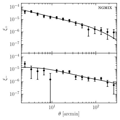
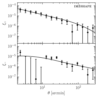
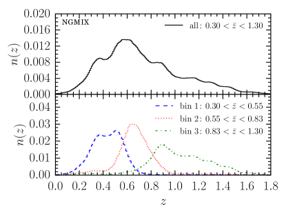
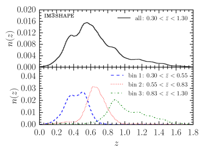
The real-space correlation functions without tomography are shown in Figure 1. We show ngmix on the left and im3shape on the right, with $\xi_{+}$ in the top rows and $\xi_{-}$ in the bottom rows. Negative measurements are shown as upper limits. The redshift distribution of sources for the non-tomographic analysis is shown in the top panel of Figure 3 for the SkyNet code. It appears in Figure 1 that the $\xi_{+}$ correlation function may approach a constant value at large scales. Interestingly, Jarvis et al. (2015) find that the mean shear across the survey for ngmix and im3shape is $\approx 7-10\times 10^{-4}$. This level of mean shear would produce a constant floor in the shear correlation functions of $\approx 5-10\times 10^{-7}$. For the DES SV survey, the root-mean-square mean shear just due to shape noise and cosmic variance is $\approx 4\times 10^{-4}$. Thus it is not clear if this feature is an indication of systematic effects or a few sigma fluctuation in the mean shear due to a real physical effect. However, in the cosmological analysis of this data, all $\xi_{+}$ data points above $60$ arcminutes were cut to avoid systematics in the PSF models (Jarvis et al., 2015; The Dark Energy Survey Collaboration et al., 2015). Thus we do not explore this issue further in this work.

We generate estimates of the $1\sigma$ uncertainties for each measurement by computing the covariance of the two-point functions over the simulation mock catalogs described in Section III. These mock catalogs are built separately for each shear catalog in order to match the non-tomographic redshift distribution of the sources. The correction factor described in Hartlap et al. (2007) is then applied to produce an unbiased estimate (see Section V.1 for a further discussion of the statistical properties of the covariance matrix estimate from the mock catalogs). The significance of the resulting measurement is then calculated from this covariance as

$$S/N=\frac{\bm{\xi}_{\rm data}\mathbf{C}^{-1}\bm{\xi}_{\rm model}}{\sqrt{\bm{\xi}_{\rm model}\mathbf{C}^{-1}\bm{\xi}_{\rm model}}},$$ (2)

where $\mathbf{C}^{-1}$ is the inverse covariance matrix estimated from the mock catalogs, $\bm{\xi}_{\rm data}$ is the vector of real-space shear two-point function measurements from the data, and $\bm{\xi}_{\rm model}$ is the vector of real-space shear two-point function measurements predicted from the cosmological model given above in Section III. This quantity corresponds to the signal-to-noise of a least-squares estimate of a scaling parameter comparing our measurements to the theoretical model. This signal-to-noise measure will be an underestimate if the model employed is not well matched to the data. However, given the good match of our fiducial model to the data as shown in Figures 1 and 2, the degree to which the signal-to-noise is underestimated is small in this case. We use the COSMOSIS package by Zuntz et al. (2015) to compute the shear correlation functions with the Takahashi et al. (2012) non-linear power spectrum fitting function. See the companion paper (The Dark Energy Survey Collaboration et al., 2015) presenting cosmological constraints from these measurements for additional details on the model correlation function $\bm{\xi}_{\rm model}$ computation. The covariance matrix has been validated through comparisons to both a detailed halo model prediction and jackknife estimates in single mock patches versus the survey data, which are discussed in detail in the Section V. We find non-tomographic cosmic shear detections at 6.5$\sigma$ and 4.7$\sigma$ significance for ngmix and im3shape respectively.

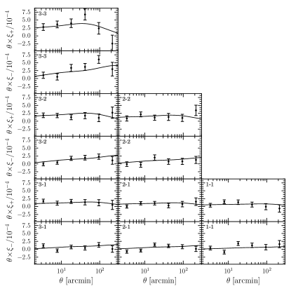
Figure 2 shows the full three-bin tomographic shear correlation function measurements for ngmix on the left and im3shape on the right. The redshift distributions of the three tomographic bins for the SkyNet code are given in the lower panels of Figure 3. In order to compute the covariance matrix of these measurements, we use the same procedure in the mock catalogs as for the non-tomographic case, except that we use the tomographic redshift distributions to assign the mock galaxies to different tomographic bins. We additionally draw the shape noise in the mock from only the galaxies in the data in the same tomographic bin. We find overall tomographic cosmic shear detections of 9.7$\sigma$ and 7.0$\sigma$ for ngmix and im3shape, respectively. Note that the ngmix catalog has more sources and extends to slightly higher redshift on average, yielding higher significance detections of cosmic shear. We have chosen three tomographic bins as a compromise between gaining signal-to-noise in the data and having too many data points in order to use the mocks to compute the covariance matrix of the data.

In Figures 1 and 2, the solid black line shows the expected amplitude and shape of the shear correlation functions in the cosmological model given above. This curve is not a fit, and is merely presented as a reference for comparison. Due to the fact that the two catalogs have different redshift distributions, a direct comparison of the shear correlation functions between the two catalogs is not possible without further work matching the two catalogs and accounting for the shared shape noise, sample variance, and image noise between the two catalogs. This matched comparison is described further in Sec. VI.2.

IV.3 Alternative Two-point Statistics

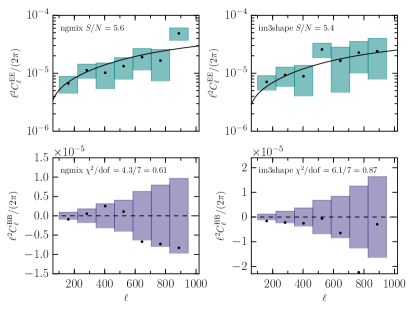
In Appendix A, we describe results from two alternative two-point statistics of the shear field. These include the methods of: (i) Becker and Rozo (2016), which use a weighting of the real-space correlation estimates to construct efficient estimates of the $C_{\ell}$ values and (ii) a second estimation of the spherical harmonic shear power spectrum using PolSpice (Szapudi et al., 2000; Chon et al., 2004). Note that these estimators weight the data at different angular scales differently than the default two-point correlation functions so that we do not expect to get identical results in terms of the significance of the cosmic shear detection. We do find detections of cosmic shear that are consistent with the conventional real-space estimators we use by default, indicating no strong preference for any given estimator. Tests of B-mode statistics from these estimators are discussed in Sec. VI.1, where we again find consistency between different two-point function estimation methods.

V Estimating and Validating the Covariance Matrix

In this section, we present our covariance matrix and a set of validation tests. The fiducial covariance matrix for our measurements is estimated from the mock catalogs presented in Section III. First we compare the covariance matrix from the mock catalogs to halo model computations. Second, we compare jackknife covariances in the data to the jackknife covariance computed from the mock catalogs. This procedure allows us to look for additional sources of noise and correlations in the data that are not present in the mock catalogs.

Figure 4: Comparison of the tomographic shear correlation function correlation matrix estimated from the mock catalogs and calculated from the halo model. The left plot shows the correlation matrix from the mock catalogs (upper left) and halo model (lower right). We show only the components for the first and last tomographic bins, plus their cross correlations. On the right, we show the square root of the diagonal elements of both covariance matrices, sorted in reverse numerical order. The open symbols show the results from the halo model and the closed symbols show the results from the mock catalogs.

Figure 5: Jackknife covariances in the mock catalogs and the data for the non-tomographic shear correlation functions. The left panel shows the correlation matrix using jackknifes in the data for ngmix (top left) and when averaging the jackknife covariances in the 126 mock catalogues (bottom right). The bottom left quadrant contains the $\xi_{+}$ correlations, the top right the $\xi_{-}$ correlations and the off diagonal components contain the cross-correlations. For each submatrix of the full correlation matrix, the angular scale increases from 2 arcminutes to 300 arcminutes. On the right, we show the diagonal elements of the jackknife covariance matrix in the data for ngmix (points) and when averaged over 126 mock catalogues (line). The grey band shows the standard deviation of diagonal elements over the 126 mock catalogs.

V.1 Simulation and Halo Model Comparison

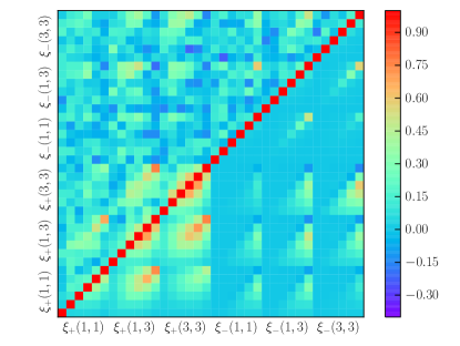
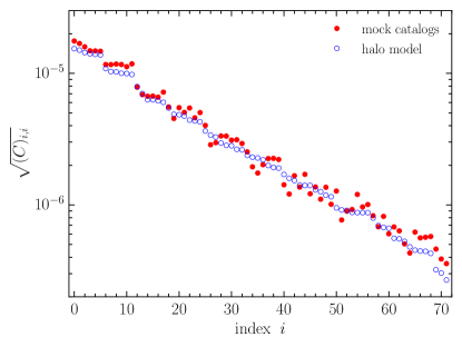
We compare the covariance matrix computed from the simulations to that obtained from a halo model in Figure 4. The simulation-based covariance matrix is computed by populating the mock catalogs with shear sources as described above in Section III, and then computing the covariance of the measurements performed on the full ensemble of mock catalogs. The halo model covariance was computed with the CosmoLike covariance module (see Eifler et al. (2014) and Krause et al. (2016) for details). Further details of our halo model computation and the full tomographic covariance matrix are given in Appendix C. Briefly, we include the Gaussian, non-Gaussian and halo sample variance terms (e.g., Takada and Hu, 2013) and compute the halo model covariance at the same cosmology and with the same redshift distribution as was used in the mock catalogs.

We compare the general structure of the mock (upper triangle) and halo model (lower triangle) covariance in the left panel of Figure 4, which shows part of the correlation matrix. Here we have shown a subset of the full set of tomographic bin combinations. The full correlation matrix is shown in Appendix C. The right panel compares the amplitude of the two covariances by plotting the variance. Overall, we find good agreement in both structure and amplitude.

We quantitatively test the agreement using a Fisher matrix computation. We compute the expected error on the degenerate parameter combination $\sigma_{8}(\Omega_{m}/0.3)^{0.5}$, where $\sigma_{8}$ is the RMS amplitude of the linear matter power spectrum at redshift zero in a top hat window of 8 $h^{-1}$Mpc and $\Omega_{m}$ is the matter density in units of the critical density at $z=0$. This combination of parameters is typically the best constrained by low-redshift cosmic shear data sets like the DES SV data. The exact degeneracy is computed in the companion cosmological constraints paper to this work (The Dark Energy Survey Collaboration et al., 2015). We use the standard Fisher matrix formalism for cosmic shear (see, e.g., Albrecht et al., 2009) and the same cosmological model as described above. We vary only the spectral index $n_{s}$, $\sigma_{8}$ and $\Omega_{m}$ in the Fisher matrix.

We find that the error bars on $\sigma_{8}(\Omega_{m}/0.3)^{0.5}$ from the halo model and mock covariances agree to approximately $10\%$ without tomography, with the halo model yielding larger parameter uncertainties. When repeating the same exercise with tomography, we find a larger, $\approx 35\%$ disagreement in the error bars, with the mocks yielding larger errors. However, we expect fluctuations in the uncertainties in parameters computed with the simulations due to the finite number of realizations used for the covariance computation. Dodelson and Schneider (2013) estimate that this effect, in the Gaussian limit, increases the variance in the parameter estimates by a factor of

$$\alpha=1+\frac{(N_{d}-N_{p})(N_{s}-N_{d}-2)}{(N_{s}-N_{b}-1)(N_{s}-N_{b}-4)}$$

where $N_{d}$ is the number of data points, $N_{s}$ is the number of simulations and $N_{p}$ is the number of parameters. This factor is $\approx 1+N_{d}/N_{s}$ in the limit that $N_{s}\gg N_{d}\gg N_{p}$. Thus we expect a fractional uncertainty in the parameter uncertainties of $\approx\sqrt{\alpha-1}$. In our case with tomography, $N_{d}=72$, $N_{s}=126$ and $N_{p}=1$. With these numbers, we get that the fractional uncertainty in the parameter uncertainty is $\approx 118\%$. Thus the disagreement of $\approx 35\%$ we find with the halo model with tomography is not statistically significant. Without tomography, we find a fractional uncertainty in the uncertainty of $\approx 56\%$, again indicating consistency.

Importantly, these numbers are the fractional uncertainty in the uncertainty. For parameter estimates, the fractional increase in the uncertainty on the parameter, equal to $\sqrt{\alpha}$, is the relevant quantity. For tomography, this fractional increase is $\approx 55\%$ and without tomography it is $\approx 15\%$. Furthermore, we have assumed that the tomographic analysis uses all 72 data points. As described in The Dark Energy Survey Collaboration et al. (2015), only 36 of the 72 data points are used for tomography, bringing the fractional increase in the error due to the finite number of realizations down to only $\approx 18\%$. Similar cuts are made for the non-tomographic analysis, using only 16 of the 30 data points. This number of data points results in a fractional increase of the parameter uncertainties of only $\approx 7\%$ for the non-tomographic analysis.

V.2 Jackknife Comparisons to Data

While our mock catalogs include both sample variance and shape noise contributions, any spatially varying systematic effects, like errors in the shear calibration, should be included in the covariance matrix of the shear correlation functions as well. To search for these potential effects, we use the jackknife covariance matrix of the shear correlation functions as a statistic to be compared between the data and the mock catalogs. Any additional sources of noise in the data, which are captured by the spatial scale of our jackknife regions, will show up as a difference between the jackknife covariance as computed in the data versus the mock catalogs.

We estimate the jackknife covariances from the data and our mock catalogs as follows. We divide both the mock catalog and data into $100$ spatial sub-regions, employing the k-means algorithm. These regions are then used to perform jackknife resampling. For the details of jackknife covariance estimation for cosmic shear correlation functions, we refer the reader to a (technical) companion paper where these choices are examined in further detail (Friedrich et al. (2016), see also Norberg et al. (2009) for an application to galaxy clustering). We use the standard jackknife scheme, where all of the shear sources in an entire subregion are removed for each jackknife resampling, which is called the galaxy-jackknife in Friedrich et al. (2016).

Note that we are not comparing jackknife covariances with the true covariances, but rather simply the co-variance in the shear correlation function across the DES SV survey to the same statistic computed with the mock catalogs. Thus the absolute correctness of the jackknife covariance matrix is not an issue for our test, since it is just a statistic that is sensitive to the effects for which we wish to search. The performance of empirical covariance measures for cosmic shear surveys is explored in Friedrich et al. (2016).

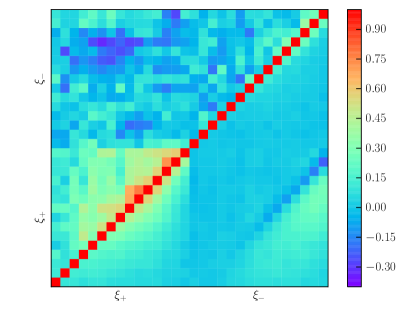
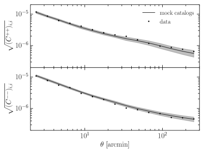
The comparison of our jackknife procedure between the mocks and the data is shown in Figure 5. Here we plot the correlation matrix of the averaged jackknife covariance from the 126 mock ngmix catalogs (left panel, on the bottom right) and the same computation in the DES SV data (on the top left). The right panel compares the diagonal elements of the jackknife covariance for $\xi_{+}$ and $\xi_{-}$ when averaged over 126 mock catalogs and when computed from the data for ngmix. Using the Fisher matrix procedure described above, we find that the error on $\sigma_{8}(\Omega_{m}/0.3)^{0.5}$ from the data jackknife covariance matrix agrees with the mean of the ensemble of errors on this parameter from the mock jackknife covariances to within one standard deviation of the error over the ensemble. Thus we conclude that there are no statistically significant sources of additional variance in the data compared to the mock catalogs.

Figure 6: Tomographic B-modes in DES SV data for ngmix (left) and im3shape (right). The error bars are calculated from the simulation realizations using the shape noise appropriate for each catalog. The tomographic bins correspond to those shown in Fig. 3 and are labeled from 1 to 3, increasing with redshift. Thus, panel ’3-2’ shows the cross-correlation between the highest and middle redshift bins. The total $\chi^{2}/{\rm d.o.f.}$, accounting for the correlations between the points in each panel, for ngmix is 62.5/60 and for im3shape is 41.2/60.

VI Tests for Residual Systematic Errors in the Cosmic Shear Signal

Systematic errors in shear measurements can be from a wide array of sources ranging from telescope optics and observing conditions to details in the modeling, measurement, and calibration of shapes. The development of tests to identify potential systematic errors is critical to verifying accurate measurement of cosmic shear. Toward this end, we devise a set of tests that should produce a null result when applied to true gravitational shear. The measurement of a significant non-zero result is then an indication of unresolved systematic errors in the shear catalog that could bias measurements.

The DES SV shear catalogs have passed a rigorous set of both traditional and novel null tests that lay the groundwork for validating the precise measurements that will be made with ongoing DES measurements during the main survey observing period. These tests are performed both at the catalog level and during the process of validating specific measurements based on the shear catalogs. We describe the methodology and results of both traditional and new null tests for sources of potential systematic errors in both the non-tomographic and tomographic measured cosmic shear signal in the next two sections.

Catalog-level tests were performed by Jarvis et al. (2015, cf. their Section 8) and included tests for additive systematic errors related to spatial position, the PSF, and galaxy properties. These tests included the cross-correlation of the galaxies and the PSF. No significant additive systematic errors were found, and they put upper limits on the potential additive systematic contribution to $\xi_{+}$ in their Section 8.7. In addition, the overall multiplicative bias of the shear estimates was tested with simulations in Jarvis et al. (2015). Jarvis et al. (2015) concludes that both catalogs are consistent with having small overall multiplicative bias, but due to uncertainties in their ability to constrain this value, they suggest marginalizing over a prior on the multiplicative bias with a standard deviation of 0.05 (see Equation 8-12 of Jarvis et al. (2015)). This multiplicative systematic is treated in the cosmological analysis of this data (The Dark Energy Survey Collaboration et al., 2015), where it contributes to an increase in the uncertainties on the final cosmological parameters constrained with this data.

VI.1 B-mode Measurements

The cosmic shear field can be characterized by E- and B-modes which differ in parity. At first-order in the gravitational potential in General Relativity, cosmic shear produces a pure E-mode field (see, e.g., Bartelmann, 2010). However, contaminating signals, like that from the telescope point-spread function, tend to contain both E- and B-modes. Thus one of the first suggested tests of cosmic shear detections was verifying that the B-mode signal is consistent with zero (Kaiser, 1992). Many methods have been suggested for B-mode estimation (e.g., Schneider et al., 1998; Seljak, 1998; Hu and White, 2001; Crittenden et al., 2002; Schneider and Kilbinger, 2007; Schneider et al., 2010). Here we use the estimators from Becker and Rozo (2016), which estimate band-powers using linear combinations of the shear two-point functions that optimally separate E- and B-modes (Becker, 2013). These estimators are

$$E=\frac{1}{2}\left[\sum f_{+i}\xi_{+i}+\sum f_{-i}\xi_{-i}\right]$$ (3)

$$B=\frac{1}{2}\left[\sum f_{+i}\xi_{+i}-\sum f_{-i}\xi_{-i}\right],$$ (4)

where the sums run over the angular bins of the shear two-point functions. The weight vectors $f_{+/-}$ are chosen to simultaneously minimize E- to B-mode mixing while also producing compact band-power estimates in Fourier-space. See Appendix A for more details.

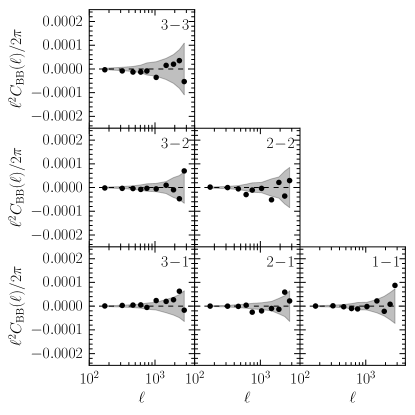
In Figure 6, we show a measurement of the tomographic B-mode signal using the Becker and Rozo (2016) band-powers. We find no statistically significant B-mode contamination, with a total $\chi^{2}/{\rm d.o.f.}$ for ngmix of 62.5/60 and for im3shape of 41.2/60. The error bars in this case are computed using the mock catalogs above. In Appendix A, we verify this conclusion by computing a complementary measurement of the non-tomographic B-mode signal using an alternate estimation of the spherical harmonic shear power spectrum. We find the B-modes from this alternate technique are consistent with zero with a $\chi^{2}/{\rm d.o.f.}=4.5/7$ for ngmix and 6.3/7 for im3shape. Finally, note that Becker and Rozo (2016) band-power measurements of the non-tomographic B-mode signal are presented in Jarvis et al. (2015) using the methods and mock catalogs of this work. The non-tomographic B-mode measurements were again found to be consistent with zero, with $\chi^{2}/{\rm d.o.f.}=22.3/20$ for ngmix and $16.1/20$ for im3shape.

VI.2 Consistency Between the Shear Pipelines

We further test for consistency between the shear catalogs split into tomographic bins by selecting only sources which pass the selection cuts for both codes. For this subset of sources, we then compare the shear auto- and cross-correlation functions for each bin. Due to the fact that the two catalogs have the same sample variance, have similar shape noise and have correlated shear measurement errors, the error bars on the difference between the two correlation functions is much smaller than that on the correlation functions themselves. We account for this effect by constructing mock catalogs where a given mock galaxy is assigned its shape noise for each shear measurement code, ngmix or im3shape, from the same real galaxy.

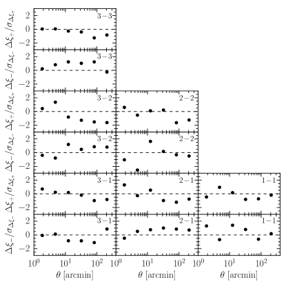
This comparison is shown in Figure 7 for the shear correlation function for im3shape minus ngmix. We find that the shear correlation functions from the codes are statistically consistent over the full range of scales from 2 to 300 arcminutes, giving a $\chi^{2}/{\rm d.o.f.}=46.8/72$. Finally, note that this test is similar to the differenced shear correlation function test presented in Section 8.6 of Jarvis et al. (2015). For their test, they examine the shear correlation function of the the difference in the ngmix and im3shape shear estimates using the matched catalogs. They find that below $\approx$3 arcminutes, the catalogs do not meet the requirements for additive systematic errors, set by the expected precision of the cosmological constraints. The test presented in this work is generally less sensitive, but complementary, to the differenced shear correlation function.

Figure 7: Difference over error in the tomographic correlation functions for matched shear catalogues from ngmix and im3shape. We show im3shape minus ngmix. The total $\chi^{2}/{\rm d.o.f.}$ accounting for all correlations is 46.8/72.

Figure 8: An example of the redshift re-weighting procedure used when comparing the correlation function between galaxies split into bins of galaxy or survey properties. Left: The SkyNet redshift distribution for each half of the ngmix data, split into upper (blue) and lower (red) bins of signal-to-noise ratio $(S/N)_{r}$ before (dashed) and after (solid) re-weighting, compared to the full sample $n(z)$ (black solid curve). Right: The distribution of weights applied to each galaxy to produce the solid $n(z)$ lines, generated as described in Sec. VI.3.

Figure 9: Null tests for the ngmix two point correlation function based on a variety of catalog and survey properties as described in Table 1. Each panel for a given property shows the difference between the $\xi_{+}$ relative to its error for the galaxies in the upper and lower halves of the sample split into bins by the magnitude of the quantity. The two halves of the sample have been reweighted to have the same redshift distribution. The error on the difference is computed directly via the mock catalogs. Grey bands are shown representing the $1\sigma$ and $2\sigma$ variance at each value of $\theta$. Adjacent points in angle are correlated.

VI.3 Two-Point Null Tests

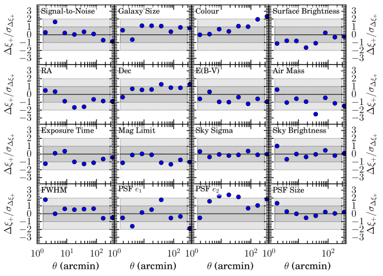
Even with a carefully chosen set of null tests at the catalog level, it is still possible that systematic errors, which can be due to complex interplays between different aspects of data and analysis, may influence the cosmic shear measurement. To test for any uncorrected systematic errors remaining in the measured cosmic shear signal, we attempt to measure the variation in $\xi_{+}$ as a function of survey and galaxy properties that may be correlated with sources systematic errors. For each survey or galaxy property, the shear data is split in half, and the correlation functions of each half are compared. We use a reweighting method to ensure that the redshift distribution of each half is the same in order to remove any cosmological dependence from this null test. If the photo-$z$s and shear measurements are correct, then the shear correlation functions of the two halves should be consistent to within the noise of the shear measurements and the redshift reweighting. If they are not, this would indicate either uncorrected systematics, selection effects from the split, or non-shear differences in the two halves such as intrinsic alignments.

Due to the fact that each half is drawn from the same area in many cases, the standard error bars computed for the shear correlation functions are not correct for this test. We instead use the mock catalogs described above to compute the error on the difference between the two halves relative to the full sample, accounting for shared sample variance, as described below. It is important to note that this is a simultaneous test of both the photometric redshifts and the shear calibrations. This feature is in fact desirable because both of these quantities can contribute to biases in the shear correlation functions. We have used both the survey property maps described by Leistedt et al. (2015) and also properties directly produced by the shape measurement codes. The 16 various systematic parameters are described in Table 1. Finally, Jarvis et al. (2015) found that making cuts on signal-to-noise and size could lead to a selection bias in the population of shear values due to preferentially selecting galaxies that look more or less like the PSF. We attempt to minimize this problem by using the “round” measures of signal-to-noise, size and surface brightness.

VI.3.1 Methodology

The galaxies in each half-sample must be reweighted so that the total $n(z)$, computed from summing the individual $p(z)$ for each galaxy according to its weight, matches between the two half-samples. Matching the redshift distributions of the two halves removes any cosmological dependence in each null test. For the data, the extra weights are computed using Ridge Regression (or Tikhonov regularization) (Pedregosa et al., 2011). We use the Ridge Regression algorithm to solve for an additional weight for each galaxy, which when used with the shear measurement weights described in Section II to compute the $n(z)$, produces a matching redshift distribution between the two half-samples. The Ridge Regression algorithm solves the linear least-squares problem with an additional regularization parameter $\alpha$, minimizing

$$||\mathbf{R}\mathbf{v}-\mathbf{t}||+||\alpha(\mathbf{v-I})||$$ (5)

where $||...||$ denotes the least-squares norm, $\mathbf{R}$ is the matrix of galaxy $p(z)$’s each weighted by the lensing weights given in Section II,

$$\mathbf{R}=\left[\begin{array}[]{lllll}w_{1}p_{11}&w_{2}p_{12}&w_{3}p_{13}&...&w_{n}p_{1n}\\ w_{1}p_{21}&w_{2}p_{22}&w_{3}p_{23}&...&w_{n}p_{2n}\\ w_{1}p_{31}&w_{2}p_{32}&w_{3}p_{33}&...&w_{n}p_{3n}\\ ...&...&...&...&...\\ w_{1}p_{m1}&w_{2}p_{m2}&w_{3}p_{m3}&...&w_{n}p_{mn}\end{array}\right]$$ (6)

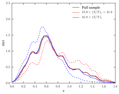
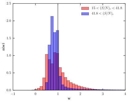
for $n$ galaxies and $m$ photo-$z$ bins with lensing weights $w_{i}$ and galaxy $p(z)$’s $p_{ji}$, $\mathbf{t}$ is the target photo-$z$ distribution, $\mathbf{v}$ is the vector of new weights for which we are solving and $\mathbf{I}$ is the identity vector. The parameter $\alpha$ governs the flexibility of the weight selection – the smaller the value, the better matched the reweighed $n(z)$ are — and is adjusted to prevent a significant contribution of negative or large weight values, which may impact the validity of the null tests. We find that $\alpha=5\times 10^{-11}$ produces an optimal match between the two half-samples while keeping the weights $\mathbf{v}$ sufficiently regular for our photo-$z$s and lensing weights. This value may not generalize to other lensing weights or photo-$z$s. We match the redshift distribution of each half-sample to that of the full sample (i.e. $\mathbf{t}$ is the redshift distribution of the full sample). This procedure is more stable than matching one half to another since smaller weights are needed for each half. The application of the Ridge Regression algorithm then produces a new weight $\mathbf{v}$, which is combined multiplicatively with the lensing weight in the calculation of the correlation functions. The resulting reweighting for galaxies split into bins of low and high galaxy detection signal-to-noise for ngmix is shown in Fig. 8. The left panel shows the $n(z)$ for each half before (dashed) and after (solid) reweighting compared to the full sample. The corresponding weight histograms are shown in the right panel.

We use the 126 DES SV-shaped mock catalogs described above to compute the variance and significance of the differences between the shear correlation functions in each half-sample. In the mock catalogs, we select a subset of galaxies in narrow redshift slices to match the $n(z)$ distribution for the full galaxy catalog. Random shape noise is generated from the shear catalog and applied to the mock catalogs, and the property with which we split the galaxy sample in half is then mapped onto the galaxies in each mock via a nearest neighbour algorithm in angular position, and redshift. This preserves the same spatial patterns as exist in the data, but the shears have been randomised so that there is no correlation with this property. We then apply the same procedure to each mock as applied to the data to directly compute the error bars on the difference via Monte Carlo, with the exception of using the true mock point redshift values to reweight the $n(z)$ histograms of each half instead of a $p(z)$ estimate for each galaxy. We expect this difference will only underestimate the variance. Any statistically significant deviations then indicate that the there may be a residual systematic error in the shear catalogs related to the quantity split upon, which has affected the measured two-point correlation function.

Figure 10: Null tests for the im3shape two point correlation function based on a variety of catalog and survey properties as described in Table 1. See Fig. 9 for details.

Property	$\chi^{2}$ $[\mathrm{d.o.f.}=8]$	$\Delta\xi_{+}/\sigma(\xi_{+})$	Description
	ngmix (im3shape)	ngmix (im3shape)
Signal-to-Noise	4.9 ( 5.2 )	0.05 ( 0.49 )	Signal-to-noise of galaxy detection
Galaxy Size	5.3 ( 10.7 )	-0.3 ( 0.15 )	Galaxy size (deconvolved with PSF)
Galaxy Colour	7.3 ( 2.2 )	-0.31 ( -0.32 )	$g-z$ colour
Surface Brightness	7.8 ( 8.7 )	0.33 ( -0.32 )	Galaxy surface brightness
RA	7.0 ( 8.8 )	0.24 ( 0.28 )	Galaxy right ascension
Dec	4.0 ( 6.2 )	-0.24 ( -0.57 )	Galaxy declination
E(B-V)	5.1 ( 6.2 )	0.23 ( 0.06 )	Mean extinction
Air Mass	20.7 ( 13.8 )	0.31 ( 0.46 )	Mean $r$-band air mass
Exposure Time	4.7 ( 6.8 )	0.18 ( 0.3 )	Mean total $r$-band exposure time
Mag. Limit	4.4 ( 7.4 )	0.18 ( 0.45 )	Mean $r$-band limiting magnitude
Sky Sigma	1.7 ( 13.0 )	-0.02 ( -0.08 )	Mean $r$-band RMS sky brightness
Sky Brightness	5.0 ( 14.3 )	-0.05 ( -0.27 )	Mean $r$-band sky brightness
FWHM	6.4 ( 3.3 )	-0.23 ( -0.13 )	Mean $r$-band PSF FWHM
PSF $e_{1}$	16.8 ( 13.5 )	0.12 ( -0.37 )	Galaxy PSF $e_{1}$
PSF $e_{2}$	17.1 ( 7.5 )	-0.58 ( -0.22 )	Galaxy PSF $e_{2}$
PSF Size	2.6 ( 5.6 )	-0.1 ( 0.42 )	Galaxy PSF size

Table 1: Summary of null tests for ngmix and im3shape. Results are given as ngmix (im3shape). The $\chi^{2}$ values are given for the differences between the two-point correlation function calculated from galaxies that fall within one of two bins in each catalog or survey property. Also shown is the magnitude of the difference relative to the 1$\sigma$ error of the measurement of $\xi_{+}$ on the full sample.

VI.3.2 Results

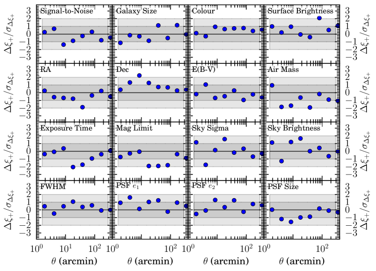
The split null tests on $\xi_{+}$ are presented in Figure 9 for ngmix and Figure 10 for im3shape. This is repeated in Appendix D for $\xi_{-}$. For each quantity (panel), the difference in $\xi_{+}$ is shown at each value of $\theta$ relative to the $1\sigma$ error in the difference from the mock catalogs. Grey bands corresponding to $1\sigma$ and $2\sigma$ errors are shown for comparison. The corresponding statistical significance of the null tests for im3shape and ngmix are given in Table 1. We find that for both ngmix and im3shape the null tests pass with deviations smaller than 2$\sigma$ ($\chi^{2}/{\rm d.o.f.}=17.8/8$) for all tests except for ngmix airmass. Note that because ngmix has a higher source density, it is generally more sensitive to residual systematic errors in these tests. While this detection is still weak, it warrants evaluating whether this difference in the galaxy population halves will have a significant bias on the correlation function. To test this, we also show in Table 1 the difference $\Delta\xi_{+}=\xi_{+({\rm upper})}-\xi_{+({\rm lower})}$ relative to the 1$\sigma$ error on the full sample measurement. For ngmix airmass, this difference is approximately one-third of the statistical error on the measurements and consistent with the level of bias in several other quantities. Of slightly lesser significance are splits in the magnitude of ngmix PSF $e_{1}$ and $e_{2}$, for which PSF $e_{2}$ has the largest difference in $\xi_{+}$ between upper and lower halves — though still small compared to the statistical error.

There is some subtlety in interpreting the significance of these null tests. First, due to physical effects not accounted for in the simulations, some tests could yield non-zero results but not indicate systematic errors in the data analysis itself. For example, if the level of intrinsic alignments differs between galaxies split by colour, then these null tests could fail and yet the shear measurements themselves could be free of systematic errors. Second, these tests could also, in principle, flag differences between the shear calibrations of galaxies of different types, which although interesting, may not ultimately impact cosmological constraints from the full sample, which could be unbiased on average. Third, as stated above, it is not clear from these tests alone if any deviations are due to the shear measurements or the photometric redshifts. Finally, note that the $\chi^{2}$ values from these tests are not independent, due to correlations in the underlying quantities used to construct the tests (e.g., the survey depth is correlated with the seeing). We have performed a large number of null tests, so to the extent that the $\chi^{2}$ values between many of the tests should be independent, we do expect some apparent deviations purely from statistical fluctuations. However, we have not attempted to combine the tests in order to quote an overall significance.

VII Conclusions

In this work, we present cosmic shear two-point measurements from Dark Energy Survey Science Verification data. We find an overall detection significance of $9.7\sigma$ for our higher source density catalog, ngmix. We additionally present multiple advances in band-power estimation, covariance estimation, simulations versus theory, and null tests for shear two-point correlations. Through this work we demonstrate that our measurements are robust and free of statistically significant systematic errors.

We demonstrate that the covariance matrices derived from the DES SV mock simulations presented in this work are consistent with the halo model, including the halo sample variance terms. We also compare the variance in the mock catalogs to the variance in the DES SV data by comparing jackknife covariances computed in the data and mock catalogs. The structure of the covariance matrices is very similar and we detect no statistically significant sources of additional variance in the data.

We find that the B-mode signals in the data are consistent with zero and that the two shear estimation codes agree well. We additionally present a set of simultaneous null tests of the photo-$z$s and shear measurements, performed by splitting the shear sample in half according to some parameter and comparing the shear correlation functions of the halves. We find that these tests pass with no statistically significant indications of biases. We expect null tests similar to those developed here to have increased utility in future cosmic shear analyses, where the statistical power is larger and the requirements for controlling systematic errors and shear selection effects are more stringent. The DES itself will have nearly $\approx 36\times$ more data and will measure cosmic shear at significantly higher signal-to-noise, so that these tests will be very useful.

Future cosmic shear two-point function measurements in the Dark Energy Survey face a variety of challenges. First, while we have a sufficient number of simulations for the SV data, simulating the increased area of the full DES will present a significant computational challenge. This challenge will need to be met by a combination of large simulation campaigns, information compression schemes applied directly to the data, and combinations of theoretical models for the covariances with simulations in order to reduce the noise in the covariance matrix elements. Second, in order to use simulations to evaluate the statistical significance of null tests on future DES data, like those presented in this work, we will need to increase the fidelity of the treatment of both the galaxies and the shear signals. Third, we must better address the formal aspects of the construction of the two-point function statistic estimators in order to make higher precision measurements. Finally, while this work has focused exclusively on broad-bin tomography of the two-point function measurements of cosmic shear, future exploration of higher order correlation functions and finer tomographic binning will be needed to extract the full amount of cosmological information from cosmic shear data. Fortunately, none of these issues are fundamentally intractable and we expect that the new techniques presented in this work will be of great assistance in making future cosmic shear measurements with DES data.

Appendix A Alternative E- and B-mode Statistics

In this appendix we consider alternative statistics of the shear field, verifying that our conclusions above, especially that the B-modes are consistent with zero, do not depend on the choice of statistic. These alternative statistics include the band-powers of Becker and Rozo (2016) and power spectra band-powers estimated with PolSpice (Szapudi et al., 2000; Chon et al., 2004).

A.1 Band-powers

The band-powers of Becker and Rozo (2016) use the methods of Becker (2013) to estimate Fourier-space band-powers directly from linear combinations of the real-space two-point functions. The final band-power estimates can be computed from the underlying E-mode power spectrum as

$$E=\int\frac{d\ln\ell\,\ell^{2}}{2\pi}C_{EE}(\ell)W_{+}(\ell)$$ (7)

where $W_{+}(\ell)$ is the band-power window function computed from the coefficients $\{f_{+i},f_{-i}\}$ in Eqs. 3 & 4. See Becker and Rozo (2016) for more details. The optimal computation of the band-powers requires computing the effective radial bin window functions of the shear correlation function points. Instead in this work we just use the geometric approximation to the bin window functions to compute the amplitudes $\{f_{+i},f_{-i}\}$. This procedure means that the band-powers do not separate E- and B-modes as well as they could in principle. However, when comparing to a fiducial cosmological model below, we do compute the band-power window function using estimates of radial bin window functions from the data. These window functions are computed via interpolating the weighted counts in each radial bin of the estimated shear two-point function. We have compared the results of this procedure for computing the window functions to estimates of the window functions from counts in finer bins. We find unsurprisingly that the bin window functions are quite smooth and thus the interpolation is accurate enough for our purpose.

Figure 11: Band-powers in DES SV data for ngmix (top) and im3shape (bottom). The error bars indicated by the grey bands are calculated from the simulation realizations using the shape noise appropriate for each catalog. The dotted lines show the band-power window functions $W_{+}(\ell)$ scaled so that their peak values are $2\times 10^{-6}$. The solid line is the prediction for the shear power spectrum for the flat, $\Lambda$CDM model given above. The dashed line shows the integral of the band-power window functions over the shear power spectrum.

Figure 12: Spherical harmonic shear power spectrum estimated using PolSpice. The left and right panels correspond to the ngmix and im3shape catalogs, respectively. The top and bottom panels show the E- and B-modes, respectively. The measurement uncertainties are estimated using the mock catalogs. The black solid lines show the predictions for the flat, $\Lambda$CDM model given above. Note that the theoretical prediction has been convolved with the PolSpice kernels, which relate the true to measured power spectra. The $S/N$ values for the E-modes are computed as outlined in Section IV.1 and the $\chi^{2}$ values for the B-modes indicate consistency with zero. The reported values take into account correlations between the band-powers.

A.2 Spherical Harmonic Power Spectrum

The cosmic shear power spectrum can also be estimated in spherical harmonic space, which has the advantage of being faster and less memory intensive than working in real-space. In view of upcoming wide field galaxy lensing surveys, e.g. the full five year DES dataset, we therefore investigate the applicability of standard spherical harmonic space methods to weak lensing. For this purpose, we use the PolSpice (Szapudi et al., 2000; Chon et al., 2004) code together with the HEALPix (Górski et al., 2005) package, which has been applied to, amongst other things, CMB polarization data (e.g., Chiang et al., 2010). PolSpice is based on the fast correlation function approach described in Szapudi et al. (2000) and Chon et al. (2004). The method is designed to exploit the advantages of both real and spherical harmonic space: to limit computation time and resources, the data are analyzed in spherical harmonic space. In order to facilitate demasking, the power spectrum is transformed to real-space in an intermediate step. In real-space, the survey mask can simply be corrected for, since the masked correlation function is the product of the unmasked correlation function and the correlation function of the mask. More precisely, the algorithm first calculates pseudo-$C_{\ell}$’s from pixelized and masked galaxy ellipticity maps which are then transformed to the correlation function. The real-space correlation function is then divided by the correlation function of the mask to correct for finite survey effects and inverted to obtain the full-sky power spectrum, removing E- to B-mode leakage in the mean. Incomplete sky coverage implies that the inversion can only be performed on angular scales for which the correlation function can be estimated thus introducing Fourier ringing in the inversion process, which can be reduced by apodizing the correlation function. Both the apodization and finite integration range introduce kernels which relate the power spectra measured by PolSpice to the underlying true power spectra. These kernels can be computed for a given apodization scheme and integration range and can therefore be corrected for when comparing measurement to theory (for details see Chon et al. (2004)).

For our analysis, we pixelize the galaxy ellipticities onto a HEALPix pixelization of the sphere with a resolution of Nside=1024, where each pixel covers a solid angle of $\approx$11.8 arcmin². In order to obtain a robust estimate of the shear field, we need to correct for multiplicative bias in the measured ellipticities. Since the correction factors described in Sections II.1 and II.2 are noisy estimates of the true corrections, we determine the mean sensitivity or multiplicative bias correction for our galaxy sample and apply this mean correction to the pixelized maps. As the power spectrum is estimated from maps constructed from the discrete values of the galaxy ellipticities, we apply a conservative masking scheme to maximize galaxy number density. We therefore adopt the DES SV LSS mask used for galaxy clustering measurements (Crocce et al., 2016). This mask is identical to the DES SV mask used for weak lensing except that it restricts analyses to the largest contiguous region overlapping the SPT-E field by selecting the area with $60<\mathrm{ra}\ [\mathrm{deg}]<95$ and $-60<\mathrm{dec}\ [\mathrm{deg}]<-40$. It further considers only regions with survey limiting magnitude in the i-band $>22.5$ (i.e. all regions considered to provide at least 10$\sigma$ measurements for objects at i-band $=22.5$; (Crocce et al., 2016)). For the power spectrum measurement, we limit all integrations to scales smaller than $\theta_{\mathrm{max}}=15$ degrees and we apodize the correlation function with a Gaussian window of $\theta_{\mathrm{FWHM}}=10$ degrees. Finally, we correct the measured power spectra for the HEALPix pixel window function and compress them into 7 band-powers with PolSpice band-power kernels.

The noise power spectrum needs to be computed from simulations. In order to produce noise only maps from the data, we remove correlations in the ellipticity maps by rotating each galaxy ellipticity by a random angle. We then estimate the noise power spectrum as the mean of the power spectra of 100 such random realizations. This procedure yields shape noise estimates consistent with $C_{\ell,\mathrm{SN}}=\frac{\sigma^{2}_{\epsilon,\mathrm{pix}}}{n_{\mathrm{pix}}}$ where $\sigma^{2}_{\epsilon,\mathrm{pix}}$ is the variance of either component of the mean ellipticity per pixel and $n_{\mathrm{pix}}$ is the angular number density of HEALPix pixels. Comparing the measured shape noise to the galaxy-based Gaussian shape noise estimate $C_{\ell,\mathrm{SN}}=\frac{\sigma^{2}_{\epsilon,\mathrm{gal}}}{n_{\mathrm{gal}}}$, where $\sigma^{2}_{\epsilon,\mathrm{gal}}$ is the variance of either component of the galaxy ellipticities and $n_{\mathrm{gal}}$ denotes the galaxy number density, we find that the latter underestimates the measured shape noise. This suggests that the galaxy ellipticity distribution is non-Gaussian and the Gaussian approximation can therefore only be applied after averaging the galaxy ellipticities over pixels. We test the pipeline using Gaussian field realizations and the mock catalogs.

A.3 Results

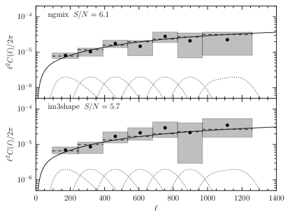
Figure 11 shows the non-tomographic band-powers using the methods of Becker and Rozo (2016), their window functions as the dotted lines, and their error bars computed with the mock catalogs as the grey bands. We find a detection significance 6.1$\sigma$ and 5.7$\sigma$ for ngmix and im3shape, respectively. These detection significances are similar to the real-space two-point functions. Finally, the solid line shows the expected shear power spectrum amplitude assuming the flat, $\Lambda$CDM model given above. The dashed line shows for each band-power the integral of the band-power window function over the shear power spectrum.

Figure 12 shows the results for the PolSpice statistics. We find a detection of cosmic shear of 5.6$\sigma$ and 5.4$\sigma$ for ngmix and im3shape respectively for the PolSpice statistics. Note that the PolSpice statistics do not use as many high-$\ell$ modes as the real-space band-powers or the real-space correlation functions, so that one expects a lower detection significance. We also find that the B-modes are statistically consistent with zero for the PolSpice statistics.

Finally, note that these two estimators process the data in different ways (e.g., averaging the data in pixels versus computing real-space correlation functions), have different sensitivities to shot noise, and have different Fourier-space window functions. We thus do not expect them to give precisely the same results in Fourier-space for the shear power spectrum. However, we do expect that when treated self-consistently they should give statistically consistent results for cosmological parameters, as demonstrated in the accompanying cosmological analysis of this data (The Dark Energy Survey Collaboration et al., 2015).  

Appendix B Validation of the Mock Catalogs

Figure 13: The shear correlation functions in the mock catalogs compared to the expected values from Takahashi et al. (2012) for all three tomographic bins (labeled in the top left corner from left to right). In the top panel, the solid lines show the theoretical expectation, the bands show the $1\sigma$ sample variance estimate and the dashed line shows the mean from the mock catalogs. $\xi_{+}$ is in red and $\xi_{-}$ is in blue. In the bottom panels, we show the fractional deviation of the mean signal in the mock catalogs from the expected values from Takahashi et al. (2012) in units of the sample variance. $\xi_{+}$ data below $\approx 2-4$ arcminutes and $\xi-$ data below $\approx 25-55$ arcminutes is not used for the final cosmological analysis in The Dark Energy Survey Collaboration et al. (2015) due to the expected baryonic effects in the matter power spectrum.

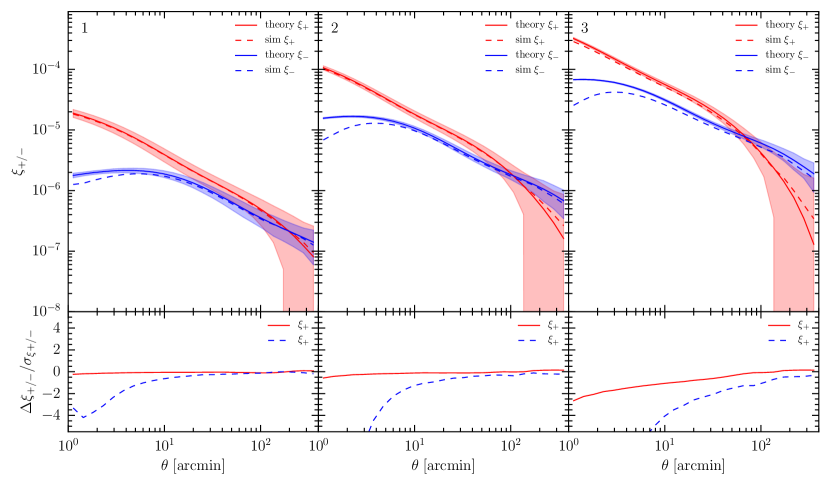
In this section we present a validation test for the mock catalogs. We compare the shear correlation functions measured in the mock catalogs in tomographic bins with the theoretical expectation from the Takahashi et al. (2012) fitting function for the matter power spectrum. The result of this test is shown in Figure 13. We find that at high redshift the small-scale shear correlation functions are suppressed relative to the theoretical expectation. Note however that this numerical effect is below the scales where the two-point functions are being used for cosmological parameter estimation ($\approx 2-4$ arcminutes for $\xi_{+}$ and $\approx 25-55$ arcminutes for $\xi_{-}$; see Table 2 of The Dark Energy Survey Collaboration et al. (2015)). Additionally, we only estimate the covariance of the two-point functions from the mock catalogs, not the mean signal. Within the noise of our mock covariance matrix, the overall parameter uncertainties are consistent when using the halo model versus the simulation covariance (see Sec. V for a quantitative comparison). This fact may indicate that the covariance is less sensitive to these numerical effects than the mean signal. Future work may require higher-resolution shear fields for covariance estimation.

Appendix C Detailed Covariance Matrix Validation

In this section, we present further details of the validation of the covariance matrices, including our tomographic halo model computations and the comparison to the simulations. The halo model covariance was computed with the CosmoLike covariance module (see Eifler et al. (2014) and Krause et al. (2016) for details).

Figure 14: Comparison of the shear correlation function correlation matrix estimated from mock catalogs and calculated from the halo model. Figure 4 shows a subset, those for tomographic bin combinations (1,1), (1,3) and (3,3), of the covariance matrix elements shown in this figure. The correlation matrix from mock catalogs is on the upper-left and that from the halo model is on the lower-right.

In the halo model, the covariance of tomographic shear power spectra $C_{\kappa}^{ij}(l)$ is given by (Cooray and Hu, 2001; Hu and Jain, 2004; Sato et al., 2009)

$$\mathrm{Cov}\left(C_{\kappa}^{ij}(l_{1}),C_{\kappa}^{kl}(l_{2})\right)=$$ (8)

$$\frac{2\pi\delta_{l_{1}l_{2}}}{\Omega_{\mathrm{s}}l_{1}\Delta l_{1}}\left[\left(C_{\kappa}^{ik}(l_{1})+\delta_{ik}\frac{\sigma_{\epsilon}^{2}}{2n^{i}}\right)\left(C_{\kappa}^{jl}(l_{2})+\delta_{jl}\frac{\sigma_{\epsilon}^{2}}{2n^{j}}\right)+\left(C_{\kappa}^{il}(l_{1})+\delta_{il}\frac{\sigma_{\epsilon}^{2}}{2n^{i}}\right)\left(C_{\kappa}^{jk}(l_{2})+\delta_{jk}\frac{\sigma_{\epsilon}^{2}}{2n^{j}}\right)\right]$$

$$+\int_{|\mathbf{l}|\in l_{1}}\frac{d^{2}\mathbf{l}}{A(l_{1})}\int_{|\mathbf{l}^{\prime}|\in l_{2}}\frac{d^{2}\mathbf{l}^{\prime}}{A(l_{2})}\left[\frac{1}{\Omega_{\mathrm{s}}}T_{\kappa,0}^{ijkl}(\mathbf{l},-\mathbf{l},\mathbf{l}^{\prime},-\mathbf{l}^{\prime})+T_{\kappa,\rm{HSV}}^{ijkl}(\mathbf{l},-\mathbf{l},\mathbf{l}^{\prime},-\mathbf{l}^{\prime})\right]\,,$$

with $n^{i}$ the number of source galaxies in tomography bin $i$, $\sigma_{\epsilon}$ the ellipticity dispersion, $A(l_{i})=\int_{|\mathbf{l}|\in l_{i}}d^{2}\mathbf{l}\approx 2\pi l_{i}\Delta l_{i}$ the integration area associated with a power spectrum bin centered at $l_{i}$ and width $\Delta l_{i}$, and $T_{\kappa,0}^{ijkl}$ and $T_{\kappa,\rm{HSV}}^{ijkl}$ the convergence trispectrum of source redshift bins $i,j,k$ and $l$ in the absence of finite volume effects and the halo sample variance contribution to the trispectrum (Sato et al., 2009; Takada and Hu, 2013). Our halo model implementation for these terms is described in Eifler et al. (2015).

Note that Equation 8 ignores the so called finite-area effect (cf. Sato et al. (2011) or Friedrich et al. (2016)), linear beat-coupling terms (e.g., Takada and Jain, 2009) and linear dilation terms Li et al. (e.g., 2014). For a survey of the size of DES-SV the finite-area effect is expected to be negligible. Furthermore, ignoring this effect is at most conservative since it will slightly overestimate the statistical uncertainties. The beat-coupling terms are negligible compared to the halo sample variance terms (and even the non-Gaussian terms, see e.g., Takada and Jain (2009)). Further, the linear dilation terms reduce the effect of the beat-coupling terms and are negligible (Li et al., 2014). Finally, we have ignored the effects of masking (except for the total area of the survey in the halo sample variance terms). We have found with Gaussian simulations that the effects of the details of the mask, besides the overall survey area, are negligible when computing cosmological constraints.

The covariance of angular shear correlation functions is then given by

$$\mathrm{Cov}\left(\xi_{\pm}^{ij}(\theta_{1}),\xi_{\pm}^{kl}(\theta_{2})\right)=\int\frac{dl}{2\pi}lJ_{0/4}\left(l\theta_{1}\right)\int\frac{dl^{\prime}}{2\pi}l^{\prime}J_{0/4}\left(l^{\prime}\theta_{2}\right)\,\mathrm{Cov}\left(C_{\kappa}^{ij}(l_{1}),C_{\kappa}^{kl}(l_{2})\right)\,$$ (9)

where we use the results of Joachimi et al. (2008) to simplify the calculation of the Gaussian part of the covariance.

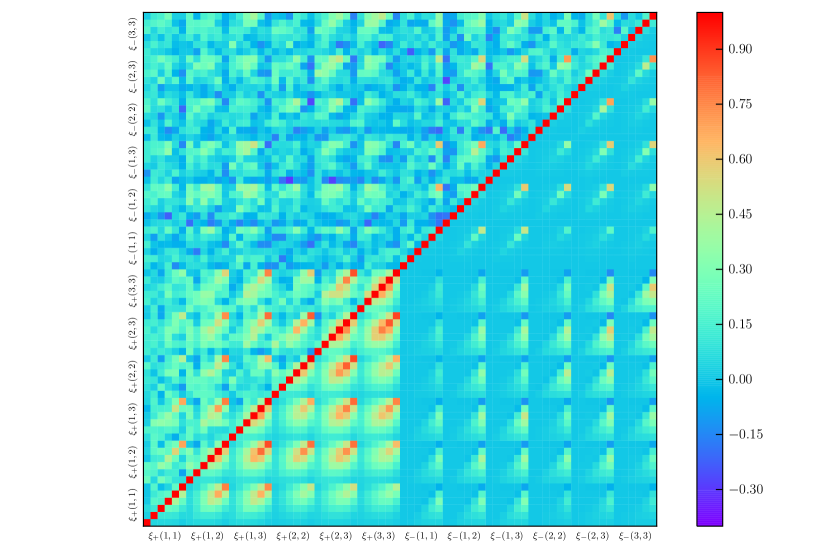
Figure 14 shows the full tomographic correlation matrix, comparing the halo model on the lower-right and the mock catalogs on the upper-left. The overall structure of the covariance matrices is similar in both computations, but the mock catalogs exhibit more noise in the off-diagonal components.

Appendix D Additional Two-Point Null Tests of $\xi_{-}$

Figure 15: Null tests for the ngmix two point correlation function based on a variety of catalog and survey properties as described in Table 1. See Fig. 9 for details.

Figure 16: Null tests for the im3shape two point correlation function based on a variety of catalog and survey properties as described in Table 1. See Fig. 9 for details.

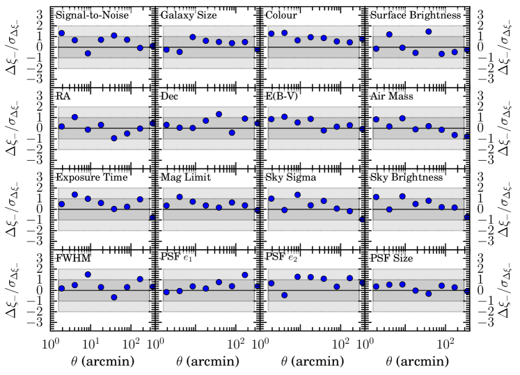
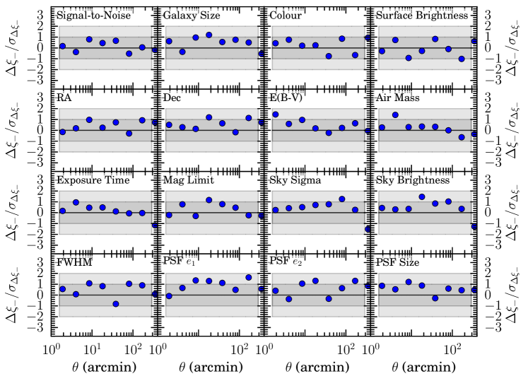
We have repeated an identical analysis for $\xi_{-}$ to that described in Sec. VI.3 for $\xi_{+}$. We show the results of the tests for im3shape in Fig. 15 and for ngmix in Fig. 16. Qualitatively, comparing to Figs. 9 & 10, there is an indication that some of the larger deviations in the figures for $\xi_{+}$ may be due to additive systematic errors. For example, there is an offset in the difference of $\xi_{+}$ based on values of airmass at the 2$\sigma$ level that disappears for $\xi_{-}$. The corresponding $\chi^{2}$ and difference values are given in Table 2. There are no significant indications of systematic errors in these null tests for $\xi_{-}$, though this may simply be due to the poorer constraining power of $\xi_{-}$.

Property	$\chi^{2}$ $[\mathrm{d.o.f.}=8]$	$\Delta\xi_{-}/\sigma(\xi_{-})$	Description
	ngmix (im3shape)	ngmix (im3shape)
Signal-to-Noise	5.8 ( 1.8 )	-0.07 ( 0.03 )	Signal-to-noise of galaxy detection
Galaxy Size	2.5 ( 5.0 )	-0.23 ( -0.35 )	Galaxy size (deconvolved with PSF)
Galaxy Colour	7.1 ( 3.8 )	-0.3 ( 0.04 )	$g-z$ colour
Surface Brightness	4.4 ( 5.2 )	-0.04 ( -0.06 )	Galaxy surface brightness
RA	2.9 ( 3.0 )	0.06 ( -0.22 )	Galaxy right ascension
Dec	4.9 ( 3.5 )	-0.35 ( -0.37 )	Galaxy declination
E(B-V)	2.8 ( 4.9 )	-0.22 ( -0.02 )	Mean extinction
Air Mass	2.7 ( 3.4 )	-0.01 ( -0.08 )	Mean $r$-band air mass
Exposure Time	4.5 ( 2.5 )	-0.35 ( 0.0 )	Mean total $r$-band exposure time
Mag. Limit	2.2 ( 3.3 )	-0.29 ( -0.43 )	Mean $r$-band limiting magnitude
Sky Sigma	3.8 ( 5.6 )	-0.21 ( -0.3 )	Mean $r$-band RMS sky brightness
Sky Brightness	4.0 ( 6.2 )	-0.27 ( -0.42 )	Mean $r$-band sky brightness
FWHM	4.1 ( 4.5 )	-0.2 ( -0.08 )	Mean $r$-band PSF FWHM
PSF $e_{1}$	2.7 ( 7.9 )	-0.37 ( -0.55 )	Galaxy PSF $e_{1}$
PSF $e_{2}$	6.8 ( 5.8 )	-0.5 ( -0.33 )	Galaxy PSF $e_{2}$
PSF Size	1.2 ( 3.8 )	-0.08 ( -0.1 )	Galaxy PSF size

Table 2: Summary of null tests for ngmix and im3shape. Results for ngmix and im3shape are given as ngmix (im3shape). The $\chi^{2}$ values are given for the differences between the two-point correlation function calculated from galaxies that fall within one of two bins in each catalog or survey property. Also shown is the magnitude of the difference relative to the 1$\sigma$ error of the measurement of $\xi_{-}$ on the full sample.

References

- The Dark Energy Survey Collaboration et al. (2015) The Dark Energy Survey Collaboration, T. Abbott, F. B. Abdalla, S. Allam, A. Amara, J. Annis, R. Armstrong, D. Bacon, M. Banerji, A. H. Bauer, E. Baxter, M. R. Becker, A. Benoit-Lévy, R. A. Bernstein, G. M. Bernstein, E. Bertin, J. Blazek, C. Bonnett, S. L. Bridle, D. Brooks, C. Bruderer, E. Buckley-Geer, D. L. Burke, M. T. Busha, D. Capozzi, A. Carnero Rosell, M. Carrasco Kind, J. Carretero, F. J. Castander, C. Chang, J. Clampitt, M. Crocce, C. E. Cunha, C. B. D’Andrea, L. N. da Costa, R. Das, D. L. DePoy, S. Desai, H. T. Diehl, J. P. Dietrich, S. Dodelson, P. Doel, A. Drlica-Wagner, G. Efstathiou, T. F. Eifler, B. Erickson, J. Estrada, A. E. Evrard, A. Fausti Neto, E. Fernandez, D. A. Finley, B. Flaugher, P. Fosalba, O. Friedrich, J. Frieman, C. Gangkofner, J. Garcia-Bellido, E. Gaztanaga, D. W. Gerdes, D. Gruen, R. A. Gruendl, G. Gutierrez, W. Hartley, M. Hirsch, K. Honscheid, E. M. Huff, B. Jain, D. J. James, M. Jarvis, T. Kacprzak, S. Kent, D. Kirk, E. Krause, A. Kravtsov, K. Kuehn, N. Kuropatkin, J. Kwan, O. Lahav, B. Leistedt, T. S. Li, M. Lima, H. Lin, N. MacCrann, M. March, J. L. Marshall, P. Martini, R. G. McMahon, P. Melchior, C. J. Miller, R. Miquel, J. J. Mohr, E. Neilsen, R. C. Nichol, A. Nicola, B. Nord, R. Ogando, A. Palmese, H. V. Peiris, A. A. Plazas, A. Refregier, N. Roe, A. K. Romer, A. Roodman, B. Rowe, E. S. Rykoff, C. Sabiu, I. Sadeh, M. Sako, S. Samuroff, C. Sánchez, E. Sanchez, H. Seo, I. Sevilla-Noarbe, E. Sheldon, R. C. Smith, M. Soares-Santos, F. Sobreira, E. Suchyta, M. E. C. Swanson, G. Tarle, J. Thaler, D. Thomas, M. A. Troxel, V. Vikram, A. R. Walker, R. H. Wechsler, J. Weller, Y. Zhang, and J. Zuntz, arXiv:astro-ph/1507.05552 (2015), arXiv:1507.05552 .
- Albrecht et al. (2006) A. Albrecht, G. Bernstein, R. Cahn, W. L. Freedman, J. Hewitt, W. Hu, J. Huth, M. Kamionkowski, E. W. Kolb, L. Knox, J. C. Mather, S. Staggs, and N. B. Suntzeff, arXiv:astro-ph/0609591 (2006), astro-ph/0609591 .
- Peacock and Schneider (2006) J. Peacock and P. Schneider, The Messenger 125, 48 (2006).
- Weinberg et al. (2013) D. H. Weinberg, M. J. Mortonson, D. J. Eisenstein, C. Hirata, A. G. Riess, and E. Rozo, Phys. Rep. 530, 87 (2013), arXiv:1201.2434 .
- Kilbinger (2015) M. Kilbinger, Reports on Progress in Physics 78, 086901 (2015), arXiv:1411.0115 .
- Bacon et al. (2000) D. J. Bacon, A. R. Refregier, and R. S. Ellis, MNRAS 318, 625 (2000), arXiv:astro-ph/0003008 .
- Kaiser et al. (2000) N. Kaiser, G. Wilson, and G. A. Luppino, arXiv:astro-ph/0003338 (2000), astro-ph/0003338 .
- Wittman et al. (2000) D. M. Wittman, J. A. Tyson, D. Kirkman, I. Dell’Antonio, and G. Bernstein, Nature 405, 143 (2000), astro-ph/0003014 .
- van Waerbeke et al. (2000) L. van Waerbeke et al., Astron. Astrophys. 358, 30 (2000), astro-ph/0002500 .
- Jee et al. (2013) M. J. Jee, J. A. Tyson, M. D. Schneider, D. Wittman, S. Schmidt, and S. Hilbert, ApJ 765, 74 (2013), arXiv:1210.2732 [astro-ph.CO] .
- Lin et al. (2012) H. Lin, S. Dodelson, H.-J. Seo, M. Soares-Santos, J. Annis, J. Hao, D. Johnston, J. M. Kubo, R. R. R. Reis, and M. Simet, ApJ 761, 15 (2012), arXiv:1111.6622 .
- Huff et al. (2014) E. M. Huff, T. Eifler, C. M. Hirata, R. Mandelbaum, D. Schlegel, and U. Seljak, MNRAS 440, 1322 (2014).
- Kuijken et al. (2015) K. Kuijken, C. Heymans, H. Hildebrandt, R. Nakajima, T. Erben, J. T. A. de Jong, M. Viola, A. Choi, H. Hoekstra, L. Miller, E. van Uitert, A. Amon, C. Blake, M. Brouwer, A. Buddendiek, I. F. Conti, M. Eriksen, A. Grado, J. Harnois-Déraps, E. Helmich, R. Herbonnet, N. Irisarri, T. Kitching, D. Klaes, F. La Barbera, N. Napolitano, M. Radovich, P. Schneider, C. Sifón, G. Sikkema, P. Simon, A. Tudorica, E. Valentijn, G. Verdoes Kleijn, and L. van Waerbeke, MNRAS 454, 3500 (2015), arXiv:1507.00738 .
- Kilbinger et al. (2013) M. Kilbinger, L. Fu, C. Heymans, F. Simpson, J. Benjamin, T. Erben, J. Harnois-Déraps, H. Hoekstra, H. Hildebrandt, T. D. Kitching, Y. Mellier, L. Miller, L. Van Waerbeke, K. Benabed, C. Bonnett, J. Coupon, M. J. Hudson, K. Kuijken, B. Rowe, T. Schrabback, E. Semboloni, S. Vafaei, and M. Velander, MNRAS 430, 2200 (2013), arXiv:1212.3338 [astro-ph.CO] .
- Heymans et al. (2013) C. Heymans, E. Grocutt, A. Heavens, M. Kilbinger, T. D. Kitching, F. Simpson, J. Benjamin, T. Erben, H. Hildebrandt, H. Hoekstra, Y. Mellier, L. Miller, L. Van Waerbeke, M. L. Brown, J. Coupon, L. Fu, J. Harnois-Déraps, M. J. Hudson, K. Kuijken, B. Rowe, T. Schrabback, E. Semboloni, S. Vafaei, and M. Velander, MNRAS 432, 2433 (2013), arXiv:1303.1808 [astro-ph.CO] .
- Heitmann et al. (2014) K. Heitmann, E. Lawrence, J. Kwan, S. Habib, and D. Higdon, ApJ 780, 111 (2014), arXiv:1304.7849 [astro-ph.CO] .
- Troxel and Ishak (2015) M. A. Troxel and M. Ishak, Phys. Rep. 558, 1 (2015), arXiv:1407.6990 .
- Kirk et al. (2015) D. Kirk, M. L. Brown, H. Hoekstra, B. Joachimi, T. D. Kitching, R. Mandelbaum, C. Sifón, M. Cacciato, A. Choi, A. Kiessling, A. Leonard, A. Rassat, and B. M. Schäfer, Space Sci. Rev. 193, 139 (2015), arXiv:1504.05465 .
- Jarvis et al. (2015) M. Jarvis, E. Sheldon, J. Zuntz, T. Kacprzak, S. L. Bridle, A. Amara, R. Armstrong, M. R. Becker, G. M. Bernstein, C. Bonnett, C. Chang, R. Das, J. P. Dietrich, A. Drlica-Wagner, T. F. Eifler, C. Gangkofner, D. Gruen, M. Hirsch, E. M. Huff, B. Jain, S. Kent, D. Kirk, N. MacCrann, P. Melchior, A. A. Plazas, A. Refregier, B. Rowe, E. S. Rykoff, S. Samuroff, C. Sánchez, E. Suchyta, M. A. Troxel, V. Vikram, T. Abbott, F. B. Abdalla, S. Allam, J. Annis, A. Benoit-Lévy, E. Bertin, D. Brooks, E. Buckley-Geer, D. L. Burke, D. Capozzi, A. Carnero Rosell, M. Carrasco Kind, J. Carretero, F. J. Castander, M. Crocce, C. E. Cunha, C. B. D’Andrea, L. N. da Costa, D. L. DePoy, S. Desai, H. T. Diehl, P. Doel, A. Fausti Neto, B. Flaugher, P. Fosalba, J. Frieman, E. Gaztanaga, D. W. Gerdes, R. A. Gruendl, G. Gutierrez, K. Honscheid, D. J. James, K. Kuehn, N. Kuropatkin, O. Lahav, T. S. Li, M. Lima, M. March, P. Martini, R. Miquel, J. J. Mohr, E. Neilsen, B. Nord, R. Ogando, K. Reil, A. K. Romer, A. Roodman, M. Sako, E. Sanchez, V. Scarpine, M. Schubnell, I. Sevilla-Noarbe, R. C. Smith, M. Soares-Santos, F. Sobreira, M. E. C. Swanson, G. Tarle, J. Thaler, D. Thomas, A. R. Walker, and R. H. Wechsler, arXiv:astro-ph/1507.05603 (2015), arXiv:1507.05603 [astro-ph.IM] .
- Bonnett et al. (2015) C. Bonnett, M. A. Troxel, W. Hartley, A. Amara, B. Leistedt, M. R. Becker, G. M. Bernstein, S. Bridle, C. Bruderer, M. T. Busha, M. Carrasco Kind, M. J. Childress, F. J. Castander, C. Chang, M. Crocce, T. M. Davis, T. F. Eifler, J. Frieman, C. Gangkofner, E. Gaztanaga, K. Glazebrook, D. Gruen, T. Kacprzak, A. King, J. Kwan, O. Lahav, G. Lewis, C. Lidman, H. Lin, N. MacCrann, R. Miquel, C. R. O’Neill, A. Palmese, H. V. Peiris, A. Refregier, E. Rozo, E. S. Rykoff, I. Sadeh, C. Sánchez, E. Sheldon, S. Uddin, R. H. Wechsler, J. Zuntz, T. Abbott, F. B. Abdalla, S. Allam, R. Armstrong, M. Banerji, A. H. Bauer, A. Benoit-Lévy, E. Bertin, D. Brooks, E. Buckley-Geer, D. L. Burke, D. Capozzi, A. Carnero Rosell, J. Carretero, C. E. Cunha, C. B. D’Andrea, L. N. da Costa, D. L. DePoy, S. Desai, H. T. Diehl, J. P. Dietrich, P. Doel, A. Fausti Neto, E. Fernandez, B. Flaugher, P. Fosalba, D. W. Gerdes, R. A. Gruendl, K. Honscheid, B. Jain, D. J. James, M. Jarvis, A. G. Kim, K. Kuehn, N. Kuropatkin, T. S. Li, M. Lima, M. A. G. Maia, M. March, J. L. Marshall, P. Martini, P. Melchior, C. J. Miller, E. Neilsen, R. C. Nichol, B. Nord, R. Ogando, A. A. Plazas, K. Reil, A. K. Romer, A. Roodman, M. Sako, E. Sanchez, B. Santiago, R. C. Smith, M. Soares-Santos, F. Sobreira, E. Suchyta, M. E. C. Swanson, G. Tarle, J. Thaler, D. Thomas, V. Vikram, and A. R. Walker, arXiv:astro-ph/1507.05909 (2015), arXiv:1507.05909 .
- Diehl (2012) H. T. Diehl, in Proceedings of the 2nd International Conference on Technology and Instrumentation in Particle Physics (TIPP 2011), Physics Procedia, Vol. 37 (2012) pp. 1332 – 1340, proceedings of the 2nd International Conference on Technology and Instrumentation in Particle Physics (TIPP 2011).
- Flaugher et al. (2012) B. L. Flaugher, T. M. C. Abbott, R. Angstadt, J. Annis, M. L. Antonik, J. Bailey, O. Ballester, J. P. Bernstein, R. A. Bernstein, M. Bonati, G. Bremer, J. Briones, D. Brooks, E. J. Buckley-Geer, J. Campa, L. Cardiel-Sas, F. Castander, J. Castilla, H. Cease, S. Chappa, E. C. Chi, L. da Costa, D. L. DePoy, G. Derylo, J. de Vincente, H. T. Diehl, P. Doel, J. Estrada, J. Eiting, A. E. Elliott, D. A. Finley, R. Flores, J. Frieman, E. Gaztanaga, D. Gerdes, M. Gladders, V. Guarino, G. Gutierrez, J. Grudzinski, B. Hanlon, J. Hao, S. Holland, K. Honscheid, D. Huffman, C. Jackson, M. Jonas, I. Karliner, D. Kau, S. Kent, M. Kozlovsky, K. Krempetz, J. Krider, D. Kubik, K. Kuehn, S. E. Kuhlmann, K. Kuk, O. Lahav, N. Langellier, A. Lathrop, P. M. Lewis, H. Lin, W. Lorenzon, G. Martinez, T. McKay, W. Merritt, M. Meyer, R. Miquel, J. Morgan, P. Moore, T. Moore, E. Neilsen, B. Nord, R. Ogando, J. Olson, K. Patton, J. Peoples, A. Plazas, T. Qian, N. Roe, A. Roodman, B. Rossetto, E. Sanchez, M. Soares-Santos, V. Scarpine, T. Schalk, R. Schindler, R. Schmidt, R. Schmitt, M. Schubnell, K. Schultz, M. Selen, S. Serrano, T. Shaw, V. Simaitis, J. Slaughter, R. C. Smith, H. Spinka, A. Stefanik, W. Stuermer, A. Sypniewski, R. Talaga, G. Tarle, J. Thaler, D. Tucker, A. R. Walker, C. Weaverdyck, W. Wester, R. J. Woods, S. Worswick, and A. Zhao, in Society of Photo-Optical Instrumentation Engineers (SPIE) Conference Series, Society of Photo-Optical Instrumentation Engineers (SPIE) Conference Series, Vol. 8446 (2012) p. 11.
- Honscheid et al. (2012) K. Honscheid, A. Elliott, J. Annis, M. Bonati, E. Buckley-Geer, F. Castander, L. daCosta, A. Fausti, I. Karliner, S. Kuhlmann, E. Neilsen, K. Patton, K. Reil, A. Roodman, J. Thaler, S. Serrano, M. Soares Santos, and E. Suchyta, in Society of Photo-Optical Instrumentation Engineers (SPIE) Conference Series, Society of Photo-Optical Instrumentation Engineers (SPIE) Conference Series, Vol. 8451 (2012) p. 12.
- Flaugher et al. (2015) B. Flaugher, H. T. Diehl, K. Honscheid, T. M. C. Abbott, O. Alvarez, R. Angstadt, J. T. Annis, M. Antonik, O. Ballester, L. Beaufore, G. M. Bernstein, R. A. Bernstein, B. Bigelow, M. Bonati, D. Boprie, D. Brooks, E. J. Buckley-Geer, J. Campa, L. Cardiel-Sas, F. J. Castander, J. Castilla, H. Cease, J. M. Cela-Ruiz, S. Chappa, E. Chi, C. Cooper, L. N. da Costa, E. Dede, G. Derylo, D. L. DePoy, J. de Vicente, P. Doel, A. Drlica-Wagner, J. Eiting, A. E. Elliott, J. Emes, J. Estrada, A. Fausti Neto, D. A. Finley, R. Flores, J. Frieman, D. Gerdes, M. D. Gladders, B. Gregory, G. R. Gutierrez, J. Hao, S. E. Holland, S. Holm, D. Huffman, C. Jackson, D. J. James, M. Jonas, A. Karcher, I. Karliner, S. Kent, R. Kessler, M. Kozlovsky, R. G. Kron, D. Kubik, K. Kuehn, S. Kuhlmann, K. Kuk, O. Lahav, A. Lathrop, J. Lee, M. E. Levi, P. Lewis, T. S. Li, I. Mandrichenko, J. L. Marshall, G. Martinez, K. W. Merritt, R. Miquel, F. Muñoz, E. H. Neilsen, R. C. Nichol, B. Nord, R. Ogando, J. Olsen, N. Palaio, K. Patton, J. Peoples, A. A. Plazas, J. Rauch, K. Reil, J.-P. Rheault, N. A. Roe, H. Rogers, A. Roodman, E. Sanchez, V. Scarpine, R. H. Schindler, R. Schmidt, R. Schmitt, M. Schubnell, K. Schultz, P. Schurter, L. Scott, S. Serrano, T. M. Shaw, R. C. Smith, M. Soares-Santos, A. Stefanik, W. Stuermer, E. Suchyta, A. Sypniewski, G. Tarle, J. Thaler, R. Tighe, C. Tran, D. Tucker, A. R. Walker, G. Wang, M. Watson, C. Weaverdyck, W. Wester, R. Woods, B. Yanny, and DES Collaboration, AJ 150, 150 (2015), arXiv:1504.02900 [astro-ph.IM] .
- Desai et al. (2012) S. Desai, R. Armstrong, J. J. Mohr, D. R. Semler, J. Liu, E. Bertin, S. S. Allam, W. A. Barkhouse, G. Bazin, E. J. Buckley-Geer, M. C. Cooper, S. M. Hansen, F. W. High, H. Lin, Y.-T. Lin, C.-C. Ngeow, A. Rest, J. Song, D. Tucker, and A. Zenteno, ApJ 757, 83 (2012), arXiv:1204.1210 [astro-ph.CO] .
- Schneider and Seitz (1995) P. Schneider and C. Seitz, A&A 294, 411 (1995), astro-ph/9407032 .
- Sheldon (2014) E. S. Sheldon, MNRAS 444, L25 (2014), arXiv:1403.7669 .
- Hogg and Lang (2013) D. W. Hogg and D. Lang, PASP 125, 719 (2013), arXiv:1210.6563 [astro-ph.IM] .
- Miller et al. (2007) L. Miller, T. D. Kitching, C. Heymans, A. F. Heavens, and L. van Waerbeke, MNRAS 382, 315 (2007), arXiv:0708.2340 .
- Mandelbaum et al. (2014) R. Mandelbaum, B. Rowe, J. Bosch, C. Chang, F. Courbin, M. Gill, M. Jarvis, A. Kannawadi, T. Kacprzak, C. Lackner, A. Leauthaud, H. Miyatake, R. Nakajima, J. Rhodes, M. Simet, J. Zuntz, B. Armstrong, S. Bridle, J. Coupon, J. P. Dietrich, M. Gentile, C. Heymans, A. S. Jurling, S. M. Kent, D. Kirkby, D. Margala, R. Massey, P. Melchior, J. Peterson, A. Roodman, and T. Schrabback, ApJS 212, 5 (2014), arXiv:1308.4982 .
- Zuntz et al. (2013) J. Zuntz, T. Kacprzak, L. Voigt, M. Hirsch, B. Rowe, and S. Bridle, MNRAS 434, 1604 (2013), arXiv:1302.0183 [astro-ph.CO] .
- Refregier et al. (2012) A. Refregier, T. Kacprzak, A. Amara, S. Bridle, and B. Rowe, MNRAS 425, 1951 (2012), arXiv:1203.5050 .
- Kacprzak et al. (2012) T. Kacprzak, J. Zuntz, B. Rowe, S. Bridle, A. Refregier, A. Amara, L. Voigt, and M. Hirsch, MNRAS 427, 2711 (2012), arXiv:1203.5049 [astro-ph.CO] .
- Sánchez et al. (2014) C. Sánchez, M. Carrasco Kind, H. Lin, R. Miquel, F. B. Abdalla, A. Amara, M. Banerji, C. Bonnett, R. Brunner, D. Capozzi, A. Carnero, F. J. Castander, L. A. N. da Costa, C. Cunha, A. Fausti, D. Gerdes, N. Greisel, J. Gschwend, W. Hartley, S. Jouvel, O. Lahav, M. Lima, M. A. G. Maia, P. Martí, R. L. C. Ogando, F. Ostrovski, P. Pellegrini, M. M. Rau, I. Sadeh, S. Seitz, I. Sevilla-Noarbe, A. Sypniewski, J. de Vicente, T. Abbot, S. S. Allam, D. Atlee, G. Bernstein, J. P. Bernstein, E. Buckley-Geer, D. Burke, M. J. Childress, T. Davis, D. L. DePoy, A. Dey, S. Desai, H. T. Diehl, P. Doel, J. Estrada, A. Evrard, E. Fernández, D. Finley, B. Flaugher, J. Frieman, E. Gaztanaga, K. Glazebrook, K. Honscheid, A. Kim, K. Kuehn, N. Kuropatkin, C. Lidman, M. Makler, J. L. Marshall, R. C. Nichol, A. Roodman, E. Sánchez, B. X. Santiago, M. Sako, R. Scalzo, R. C. Smith, M. E. C. Swanson, G. Tarle, D. Thomas, D. L. Tucker, S. A. Uddin, F. Valdés, A. Walker, F. Yuan, and J. Zuntz, MNRAS 445, 1482 (2014), arXiv:1406.4407 [astro-ph.IM] .
- Bonnett (2015) C. Bonnett, Monthly Notices of the Royal Astronomical Society 449, 1043 (2015), http://mnras.oxfordjournals.org/content/449/1/1043.full.pdf+html .
- Graff and Feroz (2013) P. Graff and F. Feroz, “SkyNet: Neural network training tool for machine learning in astronomy,” Astrophysics Source Code Library (2013), ascl:1312.007 .
- Crocce et al. (2006) M. Crocce, S. Pueblas, and R. Scoccimarro, MNRAS 373, 369 (2006), astro-ph/0606505 .
- Lewis and Bridle (2002) A. Lewis and S. Bridle, Phys. Rev. D66, 103511 (2002), astro-ph/0205436 .
- Springel (2005) V. Springel, MNRAS 364, 1105 (2005), arXiv:astro-ph/0505010 .
- Becker (2013) M. R. Becker, MNRAS 435, 1547 (2013), arXiv:1208.0068 .
- Miller et al. (2013) L. Miller, C. Heymans, T. D. Kitching, L. van Waerbeke, T. Erben, H. Hildebrandt, H. Hoekstra, Y. Mellier, B. T. P. Rowe, J. Coupon, J. P. Dietrich, L. Fu, J. Harnois-Déraps, M. J. Hudson, M. Kilbinger, K. Kuijken, T. Schrabback, E. Semboloni, S. Vafaei, and M. Velander, MNRAS 429, 2858 (2013), arXiv:1210.8201 [astro-ph.CO] .
- Jarvis et al. (2004) M. Jarvis, G. Bernstein, and B. Jain, MNRAS 352, 338 (2004), astro-ph/0307393 .
- Hartlap et al. (2007) J. Hartlap, P. Simon, and P. Schneider, A&A 464, 399 (2007), astro-ph/0608064 .
- Zuntz et al. (2015) J. Zuntz, M. Paterno, E. Jennings, D. Rudd, A. Manzotti, S. Dodelson, S. Bridle, S. Sehrish, and J. Kowalkowski, Astronomy and Computing 12, 45 (2015), arXiv:1409.3409 .
- Takahashi et al. (2012) R. Takahashi, M. Sato, T. Nishimichi, A. Taruya, and M. Oguri, ApJ 761, 152 (2012), arXiv:1208.2701 [astro-ph.CO] .
- Becker and Rozo (2016) M. R. Becker and E. Rozo, MNRAS 457, 304 (2016), arXiv:1412.3851 .
- Szapudi et al. (2000) I. Szapudi, S. Prunet, D. Pogosyan, A. S. Szalay, and J. R. Bond, arXiv:astro-ph/0010256 (2000), astro-ph/0010256 .
- Chon et al. (2004) G. Chon, A. Challinor, S. Prunet, E. Hivon, and I. Szapudi, MNRAS 350, 914 (2004), astro-ph/0303414 .
- Eifler et al. (2014) T. Eifler, E. Krause, P. Schneider, and K. Honscheid, MNRAS 440, 1379 (2014), arXiv:1302.2401 .
- Krause et al. (2016) E. Krause, T. Eifler, and J. Blazek, MNRAS 456, 207 (2016), arXiv:1506.08730 .
- Takada and Hu (2013) M. Takada and W. Hu, Phys. Rev. D 87, 123504 (2013), arXiv:1302.6994 [astro-ph.CO] .
- Albrecht et al. (2009) A. Albrecht, L. Amendola, G. Bernstein, D. Clowe, D. Eisenstein, L. Guzzo, C. Hirata, D. Huterer, R. Kirshner, E. Kolb, and R. Nichol, arXiv:astro-ph/0901.0721 (2009), arXiv:0901.0721 [astro-ph.IM] .
- Dodelson and Schneider (2013) S. Dodelson and M. D. Schneider, Phys. Rev. D 88, 063537 (2013), arXiv:1304.2593 [astro-ph.CO] .
- Friedrich et al. (2016) O. Friedrich, S. Seitz, T. F. Eifler, and D. Gruen, MNRAS 456, 2662 (2016), arXiv:1508.00895 .
- Norberg et al. (2009) P. Norberg, C. M. Baugh, E. Gaztañaga, and D. J. Croton, MNRAS 396, 19 (2009), arXiv:0810.1885 .
- Bartelmann (2010) M. Bartelmann, Class. Quant. Grav. 27, 233001 (2010), arXiv:1010.3829 [astro-ph.CO] .
- Kaiser (1992) N. Kaiser, ApJ 388, 272 (1992).
- Hilbert et al. (2009) S. Hilbert, J. Hartlap, S. D. M. White, and P. Schneider, A&A 499, 31 (2009), arXiv:0809.5035 .
- Krause and Hirata (2010) E. Krause and C. M. Hirata, A&A 523, A28 (2010), arXiv:0910.3786 [astro-ph.CO] .
- Schneider et al. (1998) P. Schneider, L. van Waerbeke, B. Jain, and G. Kruse, MNRAS 296, 873 (1998), arXiv:astro-ph/9708143 .
- Seljak (1998) U. Seljak, ApJ 506, 64 (1998), arXiv:astro-ph/9711124 .
- Hu and White (2001) W. Hu and M. White, ApJ 554, 67 (2001), arXiv:astro-ph/0010352 .
- Crittenden et al. (2002) R. G. Crittenden, P. Natarajan, U.-L. Pen, and T. Theuns, ApJ 568, 20 (2002), astro-ph/0012336 .
- Schneider and Kilbinger (2007) P. Schneider and M. Kilbinger, A&A 462, 841 (2007), arXiv:astro-ph/0605084 .
- Schneider et al. (2010) P. Schneider, T. Eifler, and E. Krause, A&A 520, A116 (2010), arXiv:1002.2136 [astro-ph.CO] .
- Leistedt et al. (2015) B. Leistedt, H. V. Peiris, F. Elsner, A. Benoit-Lévy, A. Amara, A. H. Bauer, M. R. Becker, C. Bonnett, C. Bruderer, M. T. Busha, M. Carrasco Kind, C. Chang, M. Crocce, L. N. da Costa, E. Gaztanaga, E. M. Huff, O. Lahav, A. Palmese, W. J. Percival, A. Refregier, A. J. Ross, E. Rozo, E. S. Rykoff, C. Sánchez, I. Sadeh, I. Sevilla-Noarbe, F. Sobreira, E. Suchyta, M. E. C. Swanson, R. H. Wechsler, F. B. Abdalla, S. Allam, M. Banerji, G. M. Bernstein, R. A. Bernstein, E. Bertin, S. L. Bridle, D. Brooks, E. Buckley-Geer, D. L. Burke, D. Capozzi, A. Carnero Rosell, J. Carretero, C. E. Cunha, C. B. D’Andrea, D. L. DePoy, S. Desai, H. T. Diehl, P. Doel, T. F. Eifler, A. E. Evrard, A. Fausti Neto, B. Flaugher, P. Fosalba, J. Frieman, D. W. Gerdes, D. Gruen, R. A. Gruendl, G. Gutierrez, K. Honscheid, D. J. James, M. Jarvis, S. Kent, K. Kuehn, N. Kuropatkin, T. S. Li, M. Lima, M. A. G. Maia, M. March, J. L. Marshall, P. Martini, P. Melchior, C. J. Miller, R. Miquel, R. C. Nichol, B. Nord, R. Ogando, A. A. Plazas, K. Reil, A. K. Romer, A. Roodman, E. Sanchez, B. Santiago, V. Scarpine, M. Schubnell, R. C. Smith, M. Soares-Santos, G. Tarle, J. Thaler, D. Thomas, V. Vikram, A. R. Walker, W. Wester, Y. Zhang, and J. Zuntz, arXiv:astro-ph/1507.05647 (2015), arXiv:1507.05647 .
- Pedregosa et al. (2011) F. Pedregosa, G. Varoquaux, A. Gramfort, V. Michel, B. Thirion, O. Grisel, M. Blondel, P. Prettenhofer, R. Weiss, V. Dubourg, J. Vanderplas, A. Passos, D. Cournapeau, M. Brucher, M. Perrot, and E. Duchesnay, Journal of Machine Learning Research 12, 2825 (2011).
- Górski et al. (2005) K. M. Górski, E. Hivon, A. J. Banday, B. D. Wandelt, F. K. Hansen, M. Reinecke, and M. Bartelmann, ApJ 622, 759 (2005), arXiv:astro-ph/0409513 .
- Chiang et al. (2010) H. C. Chiang, P. A. R. Ade, D. Barkats, J. O. Battle, E. M. Bierman, J. J. Bock, C. D. Dowell, L. Duband, E. F. Hivon, W. L. Holzapfel, V. V. Hristov, W. C. Jones, B. G. Keating, J. M. Kovac, C. L. Kuo, A. E. Lange, E. M. Leitch, P. V. Mason, T. Matsumura, H. T. Nguyen, N. Ponthieu, C. Pryke, S. Richter, G. Rocha, C. Sheehy, Y. D. Takahashi, J. E. Tolan, and K. W. Yoon, ApJ 711, 1123 (2010), arXiv:0906.1181 [astro-ph.CO] .
- Crocce et al. (2016) M. Crocce, J. Carretero, A. H. Bauer, A. J. Ross, I. Sevilla-Noarbe, T. Giannantonio, F. Sobreira, J. Sanchez, E. Gaztanaga, M. C. Kind, C. Sánchez, C. Bonnett, A. Benoit-Lévy, R. J. Brunner, A. C. Rosell, R. Cawthon, P. Fosalba, W. Hartley, E. J. Kim, B. Leistedt, R. Miquel, H. V. Peiris, W. J. Percival, R. Rosenfeld, E. S. Rykoff, E. Sánchez, T. Abbott, F. B. Abdalla, S. Allam, M. Banerji, G. M. Bernstein, E. Bertin, D. Brooks, E. Buckley-Geer, D. L. Burke, D. Capozzi, F. J. Castander, C. E. Cunha, C. B. D’Andrea, L. N. da Costa, S. Desai, H. T. Diehl, T. F. Eifler, A. E. Evrard, A. F. Neto, E. Fernandez, D. A. Finley, B. Flaugher, J. Frieman, D. W. Gerdes, D. Gruen, R. A. Gruendl, G. Gutierrez, K. Honscheid, D. J. James, K. Kuehn, N. Kuropatkin, O. Lahav, T. S. Li, M. Lima, M. A. G. Maia, M. March, J. L. Marshall, P. Martini, P. Melchior, C. J. Miller, E. Neilsen, R. C. Nichol, B. Nord, R. Ogando, A. A. Plazas, A. K. Romer, M. Sako, B. Santiago, M. Schubnell, R. C. Smith, M. Soares-Santos, E. Suchyta, M. E. C. Swanson, G. Tarle, J. Thaler, D. Thomas, V. Vikram, A. R. Walker, R. H. Wechsler, J. Weller, J. Zuntz, and DES Collaboration, MNRAS 455, 4301 (2016), arXiv:1507.05360 .
- Cooray and Hu (2001) A. Cooray and W. Hu, ApJ 554, 56 (2001), astro-ph/0012087 .
- Hu and Jain (2004) W. Hu and B. Jain, Phys. Rev. D 70, 043009 (2004), astro-ph/0312395 .
- Sato et al. (2009) M. Sato, T. Hamana, R. Takahashi, M. Takada, N. Yoshida, T. Matsubara, and N. Sugiyama, ApJ 701, 945 (2009), arXiv:0906.2237 [astro-ph.CO] .
- Eifler et al. (2015) T. Eifler, E. Krause, S. Dodelson, A. R. Zentner, A. P. Hearin, and N. Y. Gnedin, MNRAS 454, 2451 (2015), arXiv:1405.7423 .
- Sato et al. (2011) M. Sato, M. Takada, T. Hamana, and T. Matsubara, ApJ 734, 76 (2011), arXiv:1009.2558 .
- Takada and Jain (2009) M. Takada and B. Jain, MNRAS 395, 2065 (2009), arXiv:0810.4170 .
- Li et al. (2014) Y. Li, W. Hu, and M. Takada, Phys. Rev. D 89, 083519 (2014), arXiv:1401.0385 .
- Joachimi et al. (2008) B. Joachimi, P. Schneider, and T. Eifler, A&A 477, 43 (2008), arXiv:0708.0387 .