Order-disorder transition in the two dimensional interacting monomer-dimer model: Ising criticality

Abstract

We study the order-disorder transition of the two dimensional interacting monomer-dimer model (IMD) which has two symmetric absorbing states. To be self-contained, we first estimate numerically the dynamic exponent $z$ of the two dimensional Ising model. From the relaxation dynamics of the magnetization at the critical point, we obtain $\beta/(\nu z)=0.057~{}650(12)$, or $z=2.168~{}26(45)$, where $\beta=\frac{1}{8}$ and $\nu=1$ are exactly known exponents. We, then, compare the critical relaxation of the order parameter at the transition point of the IMD with that of the Ising model. We found that the critical relaxation exponent $\beta/(\nu z)$ is in good agreement with the Ising model, unlike the recent claim by Nam et al[JSTAT (2014), P08011]. We also claim that the Binder cumulant is not an efficient quantity to locate the order-disorder transition point of the model with two symmetric absorbing states.

1 Introduction

In two dimensions, systems with two symmetric absorbing states generally exhibit two phase transitions [1, 2, 3, 4, 5, 6]. One is the symmetry breaking order-disorder transition (SBODT) and the other is the absorbing phase transition (APT). When these two transitions coincide [7], the critical relaxation dynamics shows logarithmic behavior like the voter model [8] and, in this context, the universality class to which models with two symmetric absorbing states belong is termed as the generalized voter (GV) class [2, 9, 10].

By capturing main feature of models with two symmetric absorbing states, Al Hammal et al [2] suggested a representative Langevin equation of the GV class, which resembles the model A (according to the classification scheme of [11]) with a single component. Because the critical behavior of the model A with a single component order parameter is robust against various nonequilibrium perturbations [12, 13, 14], the SBODT, once occurring at a distinct point from the APT point, is expected to share criticality with the Ising model. This indeed was confirmed numerically for the two-dimensional interacting monomers (2DIM) model [6].

Recent numerical study of the two dimensional interacting monomer-dimer model (IMD) which also has two symmetric absorbing states, however, challenged this general picture and the SBODT of the IMD was claimed not to be the same as the Ising-type phase transition [16]. Nam et al [16] argued that non-Ising criticality can be originated from interfacial fluctuation of the third state, so-called ‘dimer’ state which is absent in the 2DIM. Hence more extensive numerical study for the IMD is desired to settle down the issue of the universality class. The purpose of this paper is to clarify the universality class of the IMD by extensive Monte Carlo simulations.

This paper is organized as follows: In section 2, the dynamic rules of the two dimensional IMD are explained. Section 3 presents simulation results. Since the relaxation dynamics of the Ising model at the critical point will play an important role in this paper, we present simulation results about the dynamic exponent of the Ising model in section 3.1. Then simulation results for the IMD are presented in section 3.2. Section 4 summarizes and concludes this work.

2 Two dimensional Interacting Monomer-Dimer Model

As a variant of a catalytic surface reaction model proposed in [17], the IMD was first introduced as a one dimensional model with two symmetric absorbing states [18] and the generalization to two dimensions was introduced and studied in [5, 16]. This section explains the dynamics of the two dimensional IMD through a simulation algorithm and introduces quantities we are interested in. Let us first denote the index of each lattice point by $\vec{n}=(i,j)$ ($i,j=1,2,\ldots,L$). Periodic boundary conditions are assumed. For convenience, a site $(i,j)$ will be called an even (odd) site if $i+j$ is even (odd).

Each site is one of three states; $A$-occupied, $B$-occupied, and vacant. Each site $\vec{n}$ is assigned a random variable $\sigma_{\vec{n}}$ which takes one of three values $1$, $0$, and $-1$ if the site is occupied by $A$ ($\sigma_{\vec{n}}=1$), occupied by $B$ ($\sigma_{\vec{n}}=0$), or vacant ($\sigma_{\vec{n}}=-1$). By $A_{\vec{n}}$ [$B_{\vec{n}}$] is denoted the number of $A$’s [$B$’s] in the nearest neighbors of site $\vec{n}$. If $\sigma_{\vec{n}}=-1$ (vacant) and $A_{\vec{n}}\neq 4$, the site $\vec{n}$ is referred to as an active site. If there is no active site, no change of configurations is allowed. In this sense, a configuration without any active site is absorbing and there are two absorbing states; all even sites are occupied by $A$ and all odd sites are vacant, and vice versa.

Now we are ready for explaining an algorithm for simulations. Let us assume that there are $N_{t}$ active sites at time $t$. We choose one of active sites at random with equal probability. Assume that site $\vec{n}=(i,j)$ is selected. With probability $p$ a ‘monomer’ $A$ attempts to adsorb at this site (monomer-event) and with probability $1-p$ a ‘dimer’ $BB$ attempts to adsorb at site $\vec{n}$ and one of nearest neighbors of $\vec{n}$ (dimer-event). For a dimer-event, the nearest neighbor site $\vec{m}$ can be either $(i+1,j)$ or $(i,j+1)$ with probability $\frac{1}{2}$. Note that even if we choose $\vec{m}$ among four nearest neighbors with equal probability, the result is the same in the sense of probability.

The change by a monomer-event is as follows. If $A_{\vec{n}}=B_{\vec{n}}=0$, that is, all nearest neighbors of site $\vec{n}$ are vacant, $A$ adsorbs at site $\vec{n}$, resulting in $\sigma_{\vec{n}}=1$. If $B_{\vec{n}}=0$ but $A_{\vec{n}}\neq 0$, the adsorption attempt is neglected and no configuration change happens, which models strong repulsion between $A$’s. If $B_{\vec{n}}\neq 0$ , we choose one site among $B$-occupied nearest neighbors of $\vec{n}$ with equal probability. Assume that site $\vec{r}$ is chosen. Then the adsorption-attempting $A$ and $B$ at site $\vec{r}$ react and form a ‘molecule’ $AB$ which desorbs in no time. This event amounts to the change of $\sigma_{\vec{r}}$ from $0$ to $-1$. In any case including dimer-events below, a ‘molecule’ $AB$ formed by reaction is always removed from the system immediately.

A change by a dimer-event is as follows. If site $\vec{m}$ is not vacant, the adsorption attempt is neglected and the configuration remains the same. Assume that site $\vec{m}$ is also vacant. There are three cases which allow for a change of the configuration.

Case I:

$A_{\vec{n}}=A_{\vec{m}}=B_{\vec{n}}=B_{\vec{m}}=0$.

Case II:

$A_{\vec{n}}\neq 0$ and $A_{\vec{m}}=B_{\vec{m}}=0$; or $A_{\vec{m}}\neq 0$ and $A_{{\vec{n}}}=B_{{\vec{n}}}=0$.

Case III:

$A_{\vec{n}}\neq 0$, $A_{\vec{m}}\neq 0$.

In all three cases, a dimer $BB$ is first dissociated into two monomers which attempt to adsorb at site ${\vec{n}}$ and ${\vec{m}}$, individually. In the case I, two $B$’s adsorb at sites $\vec{n}$ and $\vec{m}$, which gives $\sigma_{\vec{n}}=\sigma_{\vec{m}}=0$. To explain what will happen in the case II, we let $\vec{s}$ [$\vec{r}$] be the site with nonzero [zero] number of $A$’s in its nearest neighbors. Then, one $B$ adsorbs at site $\vec{r}$ and another $B$ reacts with one of $A$’s occupying nearest neighbors of $\vec{s}$. This event results in $\sigma_{\vec{r}}=0$ and $\sigma_{\vec{l}}=-1$, where $\vec{l}$ is a randomly chosen site among $A$-occupied nearest neighbors of $\vec{s}$. In the case III, two $B$’s react individually with randomly chosen $A$’s. That is, the configuration becomes $\sigma_{\vec{n}_{n}}=\sigma_{\vec{m}_{n}}=-1$, where $\vec{n}_{n}$ ($\vec{m}_{n}$) is a randomly chosen site among $A$-occupied nearest neighbors of $\vec{n}$ ($\vec{m}$). Except these cases, no configuration change happens.

After the adsorption attempt, regardless of whether it is successful or not, time increases by $1/N_{t}$.

For a given configuration, we introduce a random variable ${\cal M}$ to be called ‘staggered magnetization’ (SM) as

$${\cal M}=\frac{1}{L^{2}}\sum_{i,j}(-1)^{i+j}\sigma_{i,j}.$$ (1)

After many realizations with the same initial condition, we calculate the mean SM, $m(t)$, and the (time-dependent) Binder cumulant, $U(t)$, defined as

$$m(t)=\left\langle{\cal M}\right\rangle_{t},\quad U(t)=1-\frac{\langle{\cal M}^{4}\rangle_{t}}{3\langle{\cal M}^{2}\rangle_{t}^{2}},$$ (2)

where $\langle\ldots\rangle_{t}$ stands for the average at time $t$. At the critical point of the SBODT, $m(t)$ decays to zero as $t^{-\beta/(\nu z)}$, where $\beta$ is the critical exponent for the order parameter, $\nu$ is the correlation length exponent, and $z$ is the dynamic exponent. We will estimate $\beta/(\nu z)$ from simulations and compare it with that of the Ising model.

3 Simulation Results

3.1 Preliminary : dynamic exponent of the two dimensional Ising model

Since the main purpose of this paper is to figure out whether the SBODT of the IMD is described by the critical exponents of the Ising model, we first present simulation results for the dynamic exponent of the Ising model at criticality, to be self-contained. This subsection may be read independently of other sections. In this subsection, $\sigma$ and $m(t)$ should be understood as an Ising spin and the mean magnetization of the Ising model, respectively, and these should not be confused with the same notation for the IMD.

The Ising Hamiltonian is

$$H=-J\sum_{i,j=1}^{L}\sigma_{i,j}\left(\sigma_{i+1,j}+\sigma_{i,j+1}\right),$$ (3)

where $\sigma_{i,j}$ is the Ising spin at site $(i,j)$ and periodic boundary conditions are assumed. We remind that the critical point and energy per site at the critical point are exactly known as $K_{c}\equiv J/k_{B}T_{c}=\ln(1+\sqrt{2})/2$ and $E_{c}/J=-\ln 2/2$ [19]. For convenience, we set $J=1$ and energy is measured in unit of $J$.

We simulated the dynamics of the Ising model at the critical point, using single spin flip dynamics with the Metropolis algorithm. As an initial condition, a fully ordered state is used, that is, we set $\sigma_{i,j}=1$ for all $i,j$ at $t=0$. We measure magnetization $m(t)$, fluctuation of magnetization $V(t)$, and the energy per site $E(t)$, defined as

$$m(t) = \left\langle\frac{1}{L^{2}}\sum_{i,j}\sigma_{i,j}\right\rangle_{t},$$ (4)

$$V(t) = \left\langle\left[\frac{1}{L^{2}}\sum_{i,j}\sigma_{i,j}\right]^{2}\right\rangle_{t}-m(t)^{2},$$ (5)

$$E(t) = -\frac{1}{L^{2}}\left\langle\sum_{i,j}\sigma_{i,j}\left(\sigma_{i+1,j}+\sigma_{i,j+1}\right)\right\rangle_{t}.$$ (6)

At the critical point, the asymptotic behaviors of these quantities are (see, for example, [20])

$$m(t) = A_{m}t^{-\beta/(\nu z)}\left[1+B_{m}t^{-\chi_{m}}+o(t^{-\chi_{m}})\right],$$ (7)

$$e(t) \equiv E(t)-E_{c}=A_{e}t^{-(\nu d-1)/(\nu z)}\left[1+B_{e}t^{-\chi_{e}}+o(t^{-\chi_{e}})\right],$$ (8)

$$V(t) = A_{v}t^{(\nu d-2\beta)/(z\nu)}\left[1+B_{v}t^{-\chi_{v}}+o(t^{-\chi_{v}})\right],$$ (9)

where $d$ is the dimensions of the system ($d=2$ in this paper); $\beta=\frac{1}{8}$ and $\nu=1$ are exactly known critical exponents (see, for example, [21]); $z$ is the dynamic exponent to be determined; $A$’s and $B$’s are constants; and $\chi$’s are exponents of the leading correction-to-scaling behavior which will be called leading corrections-to-scaling exponents (LCEs). To find the dynamic exponent, we investigate the effective exponent functions (EEFs) $(b>1)$

$${\cal E}_{m}(t;b) = \frac{\ln[m(t)/m(t/b)]}{\ln b}=-\frac{1}{8z}-B_{m}\frac{b^{\chi_{m}}-1}{\ln b}t^{-\chi_{m}}+o(t^{-\chi_{m}}),$$ (10)

$${\cal E}_{e}(t;b) = \frac{\ln[e(t)/e(t/b)]}{\ln b}=-\frac{1}{z}-B_{e}\frac{b^{\chi_{e}}-1}{\ln b}t^{-\chi_{e}}+o(t^{-\chi_{e}}),$$ (11)

$${\cal E}_{v}(t;b) = \frac{\ln[V(t)/V(t/b)]}{\ln b}=-\frac{7}{4z}-B_{v}\frac{b^{\chi_{v}}-1}{\ln b}t^{-\chi_{v}}+o(t^{-\chi_{v}}).$$ (12)

Since the LCE governs how the EEF approaches the asymptotic value, it is also important to find the value of the LCE. To this end, we use the method introduced recently [22, 23]. We numerically calculate the corrections-to-scaling functions (CTSFs) $Q_{m}(t;b)$, $Q_{e}(t;b)$, $Q_{v}(t;b)$, defined as

$$Q_{m}(t;b) = \ln\left[\frac{m(t)m(t/b^{2})}{m(t/b)^{2}}\right]=B_{m}(b^{\chi}_{m}-1)^{2}t^{-\chi_{m}}+o(t^{-\chi_{m}}),$$ (13)

$$Q_{e}(t;b) = \ln\left[\frac{e(t)e(t/b^{2})}{e(t/b)^{2}}\right]=B_{e}(b^{\chi}_{e}-1)^{2}t^{-\chi_{e}}+o(t^{-\chi_{e}}),$$ (14)

$$Q_{v}(t;b) = \ln\left[\frac{V(t)V(t/b^{2})}{V(t/b)^{2}}\right]=B_{v}(b^{\chi}_{v}-1)^{2}t^{-\chi_{v}}+o(t^{-\chi_{v}}).$$ (15)

Note that the knowledge of critical indices is not necessary to find $\chi$ from $Q$. For convenience, we just drop indices like $Q(t;b)$, ${\cal E}(t;b)$, $\chi$ when we have to write EEFs, CTSFs, or LCEs collectively in the following.

To estimate the critical exponents, we use the following strategy. First note that the correct value of $\chi$ makes $Q(t;b)/(b^{\chi}-1)^{2}$ for any $b$ lie on a single curve $Bt^{-\chi}$ in the long time regime. Exploiting this feature, we adjust the value of $\chi$ until double-logarithmic plots of $Q(t;b)/(b^{\chi}-1)^{2}$ as a function of $t$ for different $b$’s lie on a single straight line. After finding $\chi$, we plot ${\cal E}(t;b)$ as a function of $\tau\equiv(b^{\chi}-1)t^{-\chi}/\ln b$ for various $b$’s. These curves should lie on a straight line in the asymptotic regime, once $\chi$ is correctly estimated. By extrapolating the straight line behavior of ${\cal E}(t;b)$, we can estimate the critical exponent.

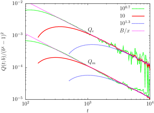
Figure 1: Double-logarithmic plots of $Q(t;b)/(b^{\chi}-1)^{2}$ vs $t$ for $b=10^{0.7}\approx 5$, $b=10$, and $b=10^{1.3}\approx 20$ (left to right) with $\chi=1$. Top three curves are for $Q_{e}(t;b)$ and bottom three curves for $Q_{m}(t;b)$. Asymptotically, curves for different $b$’s lie on a single curve, suggesting $\chi_{m}=\chi_{e}=1$. For comparison, we also plot $B/x$ with $B$ obtained from the fitting of the effective exponents; see figure 2 and figure 3.

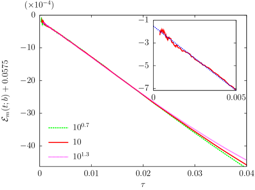
Figure 2: Plots of ${\cal E}_{m}(t;b)+0.0575$ vs $\tau\equiv(b-1)/(t\ln b)$ for $b=10^{0.7}$, 10, and $10^{1.3}$. Note that the scale on the $y$ axis is multiplied by $10^{-4}$. In the region $\tau\leq 0.02$, the effective exponents lie on a single straight line. The fitting for $\tau\leq 0.015$ of the effective exponents gives $1/(8z)=0.057~{}650(12)$ and $B_{m}=0.114(2)$. Inset: Close-up view on the region $\tau\leq 0.005$ for $b=10$ with the fitted linear function (straight line).

Now we present the simulation results. In simulations, the system size is $L=2^{12}$, the maximum observation time is $t=10^{4}$, and the number of independent runs is $2\times 10^{4}$. We begin with the analysis of $Q_{m}$ and $Q_{e}$. Figure 1 depicts $Q(t;b)/(b^{\chi}-1)^{2}$ as functions of $t$ for a few $b$’s with $\chi=1$. Since the asymptotic behavior does not depend on $b$ with the choice of $\chi=1$, the LCEs are estimated as $\chi_{m}=\chi_{e}=1$. Note that this estimate is consistent with the fitting result by Nam et al [20].

We now analyze the EEFs. Figure 2 shows how ${\cal E}_{m}(t;b)$ behaves for sufficiently large $t$, when it is depicted against $\tau\equiv(b-1)/(t\ln b)$. Since EEFs are almost on the same line irrespective of $b$ for $\tau\leq 0.02$, we conclude that the critical relaxation dynamics is well described by terms up to the leading correction for $\tau\leq 0.02$. Fitting of ${\cal E}_{m}(t;10)$ for the region $\tau\leq 0.015$ using a linear function, $1/(8z)-B_{m}\tau$ with $1/(8z)$ and $B_{m}$ to be fitting parameters, we get

$$\frac{1}{8z}=0.057~{}650(12),\quad B_{m}\approx 0.114(2),$$ (16)

or equivalently

$$z=2.168~{}26(45),$$ (17)

where the numbers in parentheses indicate the uncertainty of the last digits. We use this convention throughout the paper.

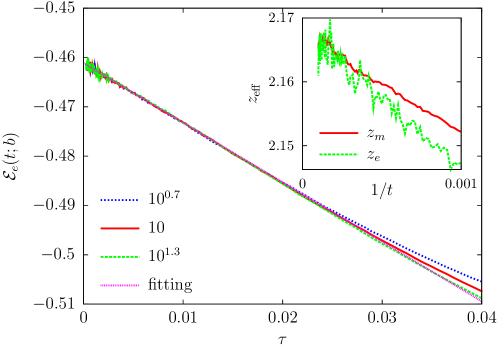
Figure 3: Plots of ${\cal E}_{e}(t;b)$ vs $\tau\equiv(b-1)/(t\ln b)$ for $b=10^{0.7}$, 10, and $10^{1.3}$. The straight line is the result of the fitting ${\cal E}_{e}(t;10)$ for the region $\tau\leq 0.015$, using a linear fitting function. Inset: Plots of $z_{\textrm{\footnotesize eff}}$ as a function of $1/t$ for the magnetization ($z_{m}$) and the energy density ($z_{e}$).

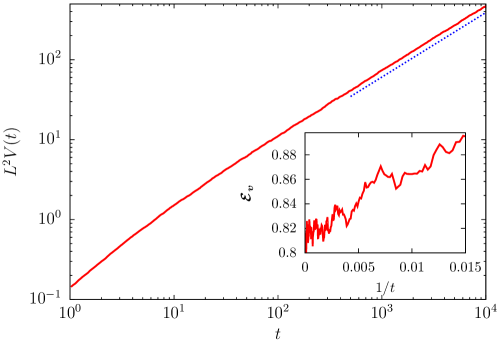
Figure 4: Log-log plot of $L^{2}V(t)$ vs $t$. A line segment with slope $7/(4z)\approx 0.8071$ is for a guide to the eyes. Inset: Plot of ${\cal E}_{v}$ vs $1/t$ for $b=10$.

Figure 3 depicts the behavior of ${\cal E}_{e}(t;b)$ for some $b$’s. Similar to ${\cal E}_{m}$, all curves for $\tau\leq 0.02$ lie on a single straight line. Due to the statistical noise of the data, the estimate of $z$ is less accurate than (17). Still, we get a consistent result within error bars. For comparison, we define effective exponents for $z$ as

$$z_{m}(t)\equiv-\frac{1}{8{\cal E}_{m}(t;10)},\quad z_{e}(t)\equiv-\frac{1}{{\cal E}_{e}(t;10)},$$ (18)

which are collectively called $z_{\textrm{\footnotesize eff}}$. The inset of figure 3 compares these two effective exponents, which shows an agreement of the limiting values of two curves within errors.

Figure 4 depicts $L^{2}V(t)$ as a function of $t$. Since $V(t)$ is the fluctuation of $m(t)$, it is not surprising that $V(t)$ is much noisier than $m(t)$. The noisy behavior of $V(t)$ becomes conspicuous when ${\cal E}_{v}$ is depicted (see the inset of figure 4). Since ${\cal E}_{v}$ is quite noisy compared to ${\cal E}_{m}$ and ${\cal E}_{e}$, the error of the estimate of the leading scaling exponent, $7/(4z)$, solely from ${\cal E}_{v}$ is larger than before. From ${\cal E}_{v}$, we estimate $7/(4z)=0.81(1)$ which is, of course, consistent with the estimate (17) within errors.

As we have seen, statistical noise is minimal when the relaxation of magnetization is investigated. Thus, we conclude $\beta/(\nu z)=0.057~{}650(12)$ and, accordingly, $z=2.168~{}26(45)$ for the single spin flip dynamics of the two dimensional Ising model with the Metropolis algorithm.

3.2 Interacting monomer-dimer model

In this section, we present the simulation results for the IMD. We begin with analyzing the EEF ${\cal E}_{m}(t)$ and the CTSF $Q_{m}(t)$ for the SM, defined similarly as (10) and (13), respectively. Since we do not know the critical point a priori, ${\cal E}_{m}(t)$ will be used to find the critical point, by exploiting the fact that ${\cal E}_{m}(t)$ should veer up (down) as $t$ gets larger if the system is in the ordered (disordered) phase.

The initial condition of simulation is that all odd sites are vacant and each even site can be either $A$-occupied with probability $m_{0}$ or vacant with probability $1-m_{0}$. With this initial preparation, the SM at time $t=0$ is $m(0)=m_{0}$. As in [16], we set $m_{0}=0.7$. Figure 5 depicts ${\cal E}_{m}$ with $b=10$ as a function of $t^{-0.75}$ for $p=0.638~{}59$ and $0.6386$. Here, the system size is $L=2^{11}$, the number of independent runs is $1400$, and the system evolves up to $t=10^{6}$. The effective exponent for $p=0.638~{}59$ [$0.6386$] approaches the Ising value (16) then veers down [up] for large $t$, suggesting that the critical point is $p_{c}=0.638~{}595(5)$. This observation shows that the critical exponent of the IMD is consistent with the Ising value, contrary to the claim in [16].

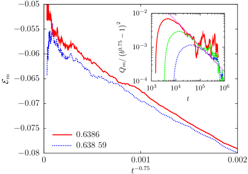
Figure 5: Plots of the effective exponents ${\cal E}_{m}$ of the SM against $t^{-0.75}$ for $p=0.638~{}59$ and $0.6386$. Here, we are using $b=10$. Inset: Log-log plots of $Q_{m}/(b^{\chi}-1)^{2}$ vs $t$ with $\chi=0.75$ for $b=10^{0.7}$, 10, $10^{1.3}$ (left to right). The straight line with the slope 0.75 is also drawn for comparison.

The inset of figure 5 shows the behavior of $Q_{m}/(b^{\chi}-1)^{2}$ at $p=0.638~{}59$ with $\chi=0.75$ for some values of $b$ on a double-logarithmic scale. Since $Q_{m}$ is measured at the disordered phase, the curves should eventually veer down [23] as can be seen at the tail of the curves in the inset. Still, the power-law region is observable and we conclude that the CSE is about 0.75. Notice that the LCSE of the IMD is smaller than that of the Ising model (see figure 1). Thus, to find the correct value of critical exponents for the IMD requires longer evolution time than the Ising model, which is also observed in [6] for the 2DIM.

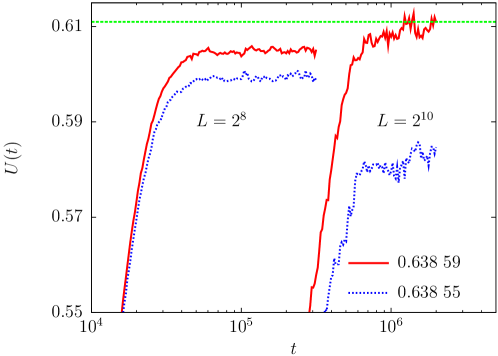
Figure 6: Plots of the time dependent Binder cumulant against $t$ on a semi-logarithmic scales for $L=2^{8}$ (left two curves) and $L=2^{10}$ (right two curves) at $p=0.638~{}55$ (top red curves) and $p=0.638~{}59$ (bottom blue curves). For comparison, a straight line indicating the critical Binder cumulant of the Ising model (0.611) is also drawn.

The study of ${\cal E}_{m}$ suggests that the order-disorder transition of the IMD is indeed described by the critical exponents of the Ising model. To support our claim further, we also study the behavior of the Binder cumulant $U(t)$. As in [16], the initial condition for the study of the Binder cumulant is the fully vacant state without any $A$ and $B$. In figure 6, we showed the behavior of $U(t)$ at $p=0.638~{}59$ (top red curves) and $p=0.638~{}55$ (bottom blue curves) for $L=2^{8}$ (left two curves) and $2^{10}$ (right two curves). The number of independent runs for $L=2^{8}$ and $p=0.638~{}55$ ($p=0.638~{}59$) is 40 000 (60 000) and the number of independent runs for $L=2^{10}$ and $p=0.638~{}55$ ($p=0.638~{}59$) is 2000 (3000). At $p=0.638~{}55$ which is the estimated critical point in [16], we also observed that $U(t)$ approaches around 0.6 for $L=2^{8}$ as in [16]. However, $U(t)$ for $L=2^{10}$ approaches 0.58, indicating that the system with $p=0.638~{}55$ is in the disordered phase. This observation is consistent with our estimate of the critical point.

As in the 2DIM studied in [6], analyzing the Binder cumulant is not an efficient method to find the critical point of the SBODT for models with two symmetric absorbing states. Even though the system with $p=0.638~{}59$ is in the disordered phase, the Binder cumulant increases up to $L=2^{10}$, which might lead to a wrong conclusion. Since the Binder cumulant at $p=0.638~{}59$ is quite close to the Ising critical value for $L=2^{10}$, to find the correct critical point using Binder cumulant requires the system size to be larger than $L=2^{10}$.

4 Summary and Conclusion

We numerically studied the two-dimensional interacting monomer-dimer model (IMD), focusing on the symmetry breaking order-disorder transition. Relaxation dynamics of the ‘staggered magnetization’ around the critical point was analyzed. The analysis of the corrections to scaling function showed that the two-dimensional IMD model has stronger corrections to scaling than the Ising model. We found that the critical point of the IMD is $p_{c}=0.638~{}595(5)$ and the relaxation dynamics at the critical point is consistent with the critical relaxation of the Ising model which is estimated as $\beta/(\nu z)=0.057~{}650(12)$ in section 3.1. Thus, we concluded that the order-disorder transition in the two dimensional IMD shares criticality with the Ising model. As a final remark, we would like to emphasize that due to strong corrections to scaling, the estimate of the critical point using the Binder cumulant becomes unreliable unless the system size is larger than $2^{10}$.

References

References

- [1] Michel Droz, Antonio L. Ferreira, and Adam Lipowski. Splitting the voter Potts model critical point. Phys. Rev. E, 67:056108, 2003.
- [2] Omar Al Hammal, Hugues Chaté, Ivan Dornic, and Miguel A . Muñoz. Langevin description of critical phenomena with two symmetric absorbing states. Phys. Rev. Lett., 94:230601, 2005.
- [3] Federico Vazquez and Cristóbal López. Systems with two symmetric absorbing states: Relating the microscopic dynamics with the macroscopic behavior. Phys. Rev. E, 78:061127, 2008.
- [4] Claudio Castellano, Miguel A . Muñoz, and Romualdo Pastor-Satorras. Nonlinear q-voter model. Phys. Rev. E, 80:041129, 2009.
- [5] Keekwon Nam, Sangwoong Park, Bongsoo Kim, and Sung Jong Lee. Double transitions, non-Ising criticality and the critical absorbing phase in an interacting monomer–dimer model on a square lattice. J. Stat. Mech.: Theory Exp., (2011):L06001, 2011.
- [6] Su-Chan Park. Order-disorder transition in a model with two symmetric absorbing states. Phys. Rev. E, 85:041140, 2012.
- [7] Man Young Lee and Thomas Vojta. Generalized contact process with two symmetric absorbing states in two dimensions. Phys. Rev. E, 83:011114, 2011.
- [8] T. M. Liggett. Interacting Particle Systems. Springer, New York, 1985.
- [9] Ivan Dornic, Hugues Chaté, Jérôme Chave, and Haye Hinrichsen. Critical coarsening without surface tension: The universality class of the voter model. Phys. Rev. Lett., 87:045701, 2001.
- [10] Léonie Canet, Hugues Chaté, Bertrand Delamotte, Ivan Dornic, and Miguel A . Muñoz. Nonperturbative fixed point in a nonequilibrium phase transition. Phys. Rev. Lett., 95:100601, 2005.
- [11] P. C. Hohenberg and B. I. Halperin. Theory of dynamic critical phenomena. Rev. Mod. Phys., 49:435, 1977.
- [12] K. E. Bassler and B. Schmittmann. Critical dynamics of nonconserved Ising-like systems. Phys. Rev. Lett., 73:3343–3346, 1994.
- [13] G Grinstein, C Jayaprakash, and H Yu. Statistical mechanics of probabilistic cellular automata. Phys. Rev. Lett., 55:2527–2530, 1985.
- [14] Uwe C. Täuber, Vamsi K. Akkineni, and Jaimie E. Santos. Effects of violating detailed balance on critical dynamics. Phys. Rev. Lett., 88:045702, 2002.
- [15] Sreedhar B. Dutta and Su-Chan Park. Critical dynamics of nonconserved -vector models with anisotropic nonequilibrium perturbations. Phys. Rev. E, 83:011117, 2011.
- [16] Keekwon Nam, Bongsoo Kim, and Sung Jong Lee. Nonequilibrium critical dynamics of two dimensional interacting monomer-dimer model: non-Ising criticality. J. Stat. Mech.: Theory Exp., (2014):P08011, 2014.
- [17] Robert M. Ziff, Erdagon Gulari, and Yoav Barshad. Kinetic phase transitions in an irreversible surface-reaction model. Phys. Rev. Lett., 56:2553–2556, 1986.
- [18] Mann Ho Kim and Hyunggyu Park. Critical behavior of an interacting monomer-dimer model. Phys. Rev. Lett., 73:2579–2582, 1994.
- [19] Lars Onsager. Crystal statistics. I. a two-dimensional model with an order-disorder transition. Phys. Rev., 65:117–149, 1944.
- [20] Keekwon Nam, Bongsoo Kim, and Sung Jong Lee. Nonequilibrium critical relaxation of the order parameter and energy in the two-dimensional ferromagnetic Potts model. Phys. Rev. E, 77:056104, 2008.
- [21] R. Baxter. Exactly Solved Models in Statistical Mechanics. Academic, New York, 1982.
- [22] Su-Chan Park. High-precision estimate of the critical exponents for the directed Ising universality class. J. Kor. Phys. Soc., 62:469–474, 2013.
- [23] Su-Chan Park. Critical decay exponent of the pair contact process with diffusion. Phys. Rev. E, 90:052115, 2014.