Phase diagram of a quantum Coulomb wire

Abstract

We report the quantum phase diagram of a one-dimensional Coulomb wire obtained using the path integral Monte Carlo (PIMC) method. The exact knowledge of the nodal points of this system permits us to find the energy in an exact way, solving the sign problem which spoils fermionic calculations in higher dimensions. The results obtained allow for the determination of the stability domain, in terms of density and temperature, of the one-dimensional Wigner crystal. At low temperatures, the quantum wire reaches the quantum-degenerate regime, which is also described by the diffusion Monte Carlo method. Increasing the temperature the system transforms to a classical Boltzmann gas which we simulate using classical Monte Carlo. At large enough density, we identify a one-dimensional ideal Fermi gas which remains quantum up to higher temperatures than in two- and three-dimensional electron gases. The obtained phase diagram as well as the energetic and structural properties of this system are relevant to experiments with electrons in quantum wires and to Coulomb ions in one-dimensional confinement.

Few systems are more universal than electron gases. Their study started long-time ago and the compilation of knowledge that we have now at hand is very wide, with impressive quantitative and qualitative results giuliani . Phase diagrams for the electron gas in two and three dimensions appear now quite well understood thanks to progressively more accurate many-body calculations using mainly quantum Monte Carlo methods ceperley_rev . However, the theoretical knowledge of the electron gas in the one-dimensional (1D) geometry is more scarce and a full determination of the density-temperature phase diagram is still lacking. The present work is intended as a contribution towards filling this gap by means of a microscopic approach based on the path integral Monte Carlo (PIMC) method.

The quasiparticle concept introduced by Landau in his Fermi liquid theory is able to account for the excitations of the electron gas in two and three dimensions. This is not the case in one dimension where the enhancement of correlations makes all excitations, even at low energy, to be collective. The appropriate theoretical framework is an effective low-energy Tomonaga-Luttinger (TL) theory tomonaga ; luttinger ; haldane , properly modified by Schulz schulz to account for the long-range nature of the Coulomb interaction. Probably, the most noticeable prediction of the TL theory is the separation between spin and charge degrees of freedom, whose excitations are predicted to travel at different velocities. At the same time, a Coulomb wire is fundamentally different from other TL systems in that at low densities it forms a Wigner crystal, as manifested by the emergence of quasi-Bragg peaks schulz . Also the strongly repulsive nature of interactions might lead to a formation of a Coulomb Tonks-Girardeau gasCTG . In spite of the experimental difficulties in getting real 1D environments, strong evidences of having reached the TL liquid and the 1D Wigner crystal have been reported in the last years pouget ; goni ; auslaender ; kim ; jompol ; laroche ; deshpande . Therefore, the continued theoretical interest on this 1D system is completely justified and can help to understand future experimental findings.

The ground-state properties of the 1D Coulomb gas have been studied in the past using several methods, the most accurate results being obtained using the diffusion Monte Carlo (DMC) method casula1 ; casula2 ; lee . One of the main goals of these calculations was the estimation of the interaction energy of the gas with as higher precision as possible to generate accurate density functionals to be used within density functional theory of quasi-one-dimensional systems. All these calculations have been carried out assuming a quasi-1D geometry imposed by a tight transverse confinement, normally of harmonic type. In the latter case, one assumes that electrons occupy the ground-state of the transverse harmonic potential and so in the resulting effective Coulomb interaction the divergence at $x=0$ is eliminated. Proceeding in this way, the effective one-dimensional interatomic potential can be Fourier transformed. However, a recent DMC calculation astra has shown that the use of the bare Coulomb interaction is not a problem for the estimation of the energy and structural properties because the wave function becomes zero when $|x|\rightarrow 0$. More importantly, the presence of a node at $x=0$ makes Girardeau’s mapping applicable girardeau which means that the many-particle bosonic wave function is the absolute value of the fermionic one, with the same Hamiltonian. In other words, the non-integrable divergence of the interaction at small distances acts effectively as a Pauli principle for bosons. From the computational point of view, this is highly relevant because knowing the exact position of the nodes allows us to perform an exact simulation without the usual upper-bound restriction imposed by the fixed-node approximation when the nodal surfaces are unknown.

We consider a system composed of $N$ particles with charge $e$ and mass $m$ in a 1D box of length $L$ with periodic boundary conditions, that interact by means of a pure Coulomb potential. We work in atomic units, the Bohr radius $a_{0}=\hbar^{2}/(me^{2})$ for the length and the Hartree $\text{Ha}=e^{2}/a_{0}$ for the energy. In these reduced units, the Hamiltonian is given by

$$H=-\frac{1}{2}\sum_{i=1}^{N}\frac{\partial^{2}}{\partial x_{i}^{2}}+\sum_{i<j}^{N}\frac{1}{|x_{i}-x_{j}|}\ .$$ (1)

At finite temperature $T$, the knowledge of the partition function $Z=\mathrm{Tr}\,e^{-\beta H}$ ($\beta=1/T$) gives access to a microscopic description of the properties of the system. The partition function satisfies a convolution property which allows for its estimation via a path integral Monte Carlo (PIMC) scheme,

$$Z=\int d{\bf R}_{1}\ldots d{\bf R}_{M}\prod_{\alpha=1}^{M}\rho({\bf R}_{\alpha},{\bf R}_{\alpha+1})\ ,$$ (2)

where $\rho({\bf R}_{\alpha},{\bf R}_{\alpha+1})$ stands for an approximated density matrix at higher temperature $MT$. In the present work, we use a fourth-order approximation for $\rho$ Chin that has already proved its efficiency in the study of other systems such as liquid ${}^{4}\mathrm{He}$ HighOrder . Here, the fourth-order dependence of the energy on $1/M$ is recovered at larger $M$ values than in ${}^{4}\mathrm{He}$ due to the pathological behavior of the Coulomb potential for the lowest approximation for the action (primitive approximation) broughton . Nevertheless, the high-order PIMC method is able to explore the major part of the density-temperature phase diagram with accuracy and without any bias coming from the fixed-node constraint.

Our main goal is the calculation of the phase diagram of the 1D Coulomb quantum wire. To this end, we mainly determine the energetic and structure properties of this system. For the energy we use the virial estimator, which relies on the invariance of the partition function under a scaling of the coordinate variables, thus providing good results at large values of $M$, where the thermodynamic estimator fails to provide converged results HighOrder . The structure properties of the system are obtained from the behavior of the static structure factor, $S(k)=N^{-1}\langle\hat{\rho}_{k}\hat{\rho}_{-k}\rangle$, with $\hat{\rho}_{k}=\sum_{l=1}^{N}\exp(ikx_{l})$ the density operator.

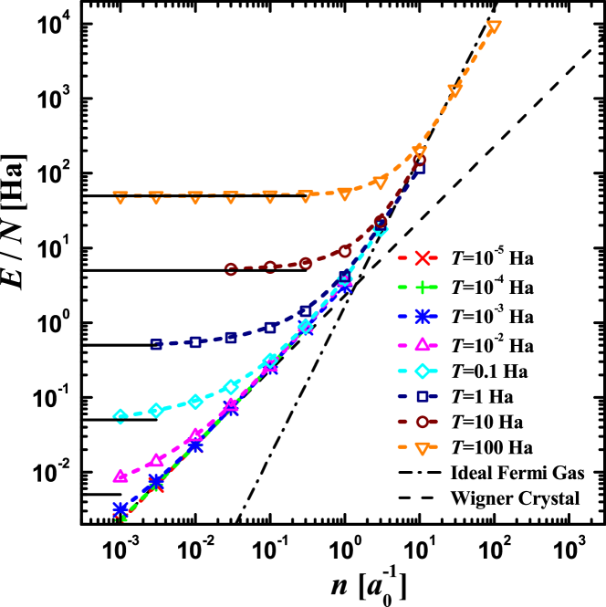
Figure 1: (Color online) Energy per particle as a function of the density for $N=10$. Symbols, PIMC results at different temperatures; dashed line, energy of a Wigner crystal at $T=0$; dash-dotted line, IFG energy at $T=0$. Solid lines, classical limit $E/N=T/2$.

The energies obtained at different temperatures and densities are shown in Fig. 1. When both the temperature and density are low, the potential energy dominates and the total energy can be estimated by summing up all pair Coulomb potential energies for a set of particles at the fixed positions of a Wigner crystal. For a given number of particles $N$, the leading term in the energy is linear with the density $n$ dubin ,

$$\frac{E_{\text{W}}}{N}=e^{2}n\ln N\ .$$ (3)

If one fixes the density and changes the number of particles, Eq. (3) predicts an energy per particle which diverges logarithmically with $N$. This is, in fact, a well known effect of the long-range behavior of the Coulomb potential in strictly 1D problems astra . When the density increases, the kinetic energy increases faster than the potential energy due to its quadratic dependence with $n$. Then, the system reaches a regime where the energy is well approximated by the ground-state energy of an ideal Fermi gas,

$$\frac{E_{\text{ IFG}}}{N}=\frac{\hbar^{2}k_{F}^{2}}{6m}\ ,$$ (4)

with $k_{F}=\pi n$ being the 1D one-component Fermi momentum. Both limiting behaviors, $E_{\text{W}}/N$ (3) and $E_{\text{ IFG}}/N$ (4) are shown as straight lines which cross at $n\simeq 1$ in the log-log plot of Fig. 1. The ground-state energy obtained with the DMC method for $T=0$ is recovered in our PIMC simulation when the temperature drops below some critical temperature, which value depends on the density. Increasing the density in the ground state, the system evolves from a Wigner crystal to a zero-temperature ideal Fermi gas astra . For a fixed finite temperature, $T\lesssim 1$ Ha, the dilute regime of low density corresponds to a classical gas with the energy per particle given by the classical value $E_{\text{C}}=T/2$ (solid horizontal lines) , the Wigner crystal is realized at larger densities and, finally, the quantum wire behaves as an ideal Fermi gas for $n\gtrsim 1$. For temperatures $T\gtrsim 1$ Ha, the Wigner crystal behavior is no more observed and the system evolves directly from a classical gas to a Fermi one.

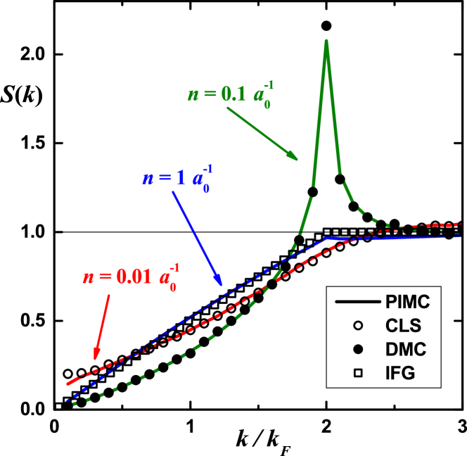
Figure 2: (Color online) Static structure factor for $N=20$ and $T=10^{-2}$ Ha for different densities. At the lowest density, we compare the PIMC result with a classical Monte Carlo simulation (CLS). For densities $n\geq 0.1\,a_{0}^{-1}$, we make a comparison with the ground-state properties obtained by the DMC method ($T=0$). For densities $n\geq 1\,a_{0}^{-1}$, we compare the PIMC results with the Ideal Fermi Gas.

In spite of the absence of real phase transitions in this 1D system one can identify different regimes with well-known limiting cases. As we have shown in Fig. 1, the energy shows a rich variety of behaviors as both the density and temperature are changed. However, it is the study of the structural properties which provides us a deeper understanding on the difference between regimes. To this end, we use the PIMC method to calculate the density and temperature dependence of the static structure factor $S(k)$. Its behavior at a constant temperature ($T=10^{-2}$ Ha) and different densities is shown in Fig. 2. At the lowest density $n=0.01\,a_{0}^{-1}$, the quantum PIMC results are nearly indistinguishable of the classical $S(k)$ obtained by the classical Monte Carlo method (Boltzmann distribution) at the same density and temperature. Increasing more the density, the static structure factor shows clearly the emergence of a Bragg peak at $k/k_{F}=2$ signaling the formation of a Wigner crystal in 1D schulz . At low temperatures, the quantum degeneracy is reached and $S(k)$ agrees with that of a DMC estimation at $T=0$ at the same density. Similarly to what happens at zero temperature astra , increasing even more the density the system evolves to an ideal Fermi gas. In Fig. 2, we also compare the PIMC result for $S(k)$ at $n=1\,a_{0}^{-1}$ with the IFG $S(k)$ at the same density and $T=0$: the agreement between both curves is excellent.

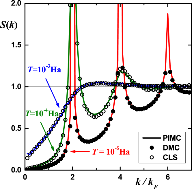
Figure 3: (Color online) Static structure factor for $N=20$ and $n=10^{-3}$ for different temperatures. At the lowest temperature we compare the PIMC result with the DMC result of $T=0$. At high temperature, we compare the PIMC result with a classical Monte Carlo simulation (CLS).

It is important to understand how the temperature affects the structural properties, when the density is fixed and the temperature is progressively increased. Figure 3 reports PIMC results obtained at low density, $n=10^{-3}\,a_{0}^{-1}$. At low temperatures, one identifies the characteristic Bragg peaks at $k/k_{F}=2l$ with integer $l$. At the lowest considered temperature, $T=10^{-5}$ Ha, we observe a quantum crystal and $S(k)$ is in nice agreement with the $T=0$ result obtained by the DMC method. Increasing the temperature by a factor of ten, the presence of Bragg peaks confirms the formation of a Wigner crystal while its structure is very different from the quantum one, observed at $T=0$. Importantly, we find out that the correlations at $T=10^{-4}$ Ha are the same as in a crystal with electrons obeying Boltzmann statistics.

Once in the classical regime, by increasing the temperature the crystal melts and becomes a gas. In Fig. 3, one can observe that PIMC and classical simulations predict the same $S(k)$ in a gas at temperature $T=10^{-3}$ Ha. It becomes clear from Figs. 2 and 3 that the transition between different regimes can be induced by changing the density or the temperature.

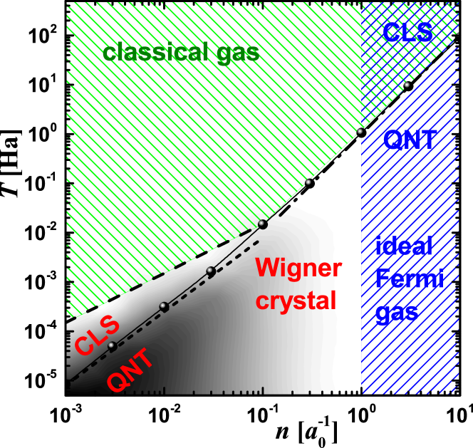
Figure 4: (Color online) Temperature – density phase diagram. Long-dashed line, gas-Wigner crystal crossover; dash-dotted line, locates the crossover between a quantum Fermi gas and a classical thermal gas ($T_{F}\propto n^{2}$); short-dashed line separates the classical (CLS) and quantum (QNT) regimes within the Wigner crystal, $T\propto n^{3/2}$; symbols connected with a thin line (guide to an eye), position of the classical-quantum crossover estimated as $E_{\text{kin}}=T$. Ideal Fermi gas and Wigner crystal regimes for the considered number of particles are separated by $n\approx 1$. Within the Wigner phase, the ratio of the peak value in $S(k)$ for $N=20$ and $N=10$ is shown with a contour plot (white color, no difference; black, large difference).

From the PIMC results for both energy and structure we establish the temperature-density phase diagram of the 1D Coulomb wire. The phase diagram is reported in Fig. 4 and constitutes the main result of our work. We identify three different regimes: classical Coulomb gas, Wigner crystal and ideal Fermi gas, where the last two regimes show a crossover from quantum to classical behavior. The Wigner crystal is identified by calculating the ratio of the peak’s height of $S(k)$ at $k/k_{F}=2$ for two values of the number of particles ($N=20$, 10). When the height of the peak increases with $N$, the system behaves as a Wigner crystal. In Fig. 4, we use a contour plot to show that ratio in a grey scale, where black color stands for large ratio and white for ratio equal to one. In the $T$-$n$ plane, the Wigner crystal phase shows a triangular shape, with the strongest signal localized in the vertex of lowest density and temperature, delimited by transitions to a Coulomb or an ideal Fermi gas. This quantum Wigner crystal is well described by the zero-temperature theory, as we have shown in Figs. 2 and 3. Increasing the temperature, one can see how the quantum crystal transforms into a classical Wigner lattice. In both regimes, particles move around the lattice points but these fluctuations are of quantum and thermal nature in quantum and classic crystals, respectively. Starting from a high-temperature crystal and by decreasing the temperature we see that the system becomes more ordered and the height of the peaks increases. Indeed, at zero temperature the classical system would always form a perfect crystal with no fluctuations. Instead, we see that the height of the peaks stops growing when we decrease the temperature down to the quantum-degeneracy regime. By lowering the temperature further the system remains in the ground state. In fact, the classical crystal regime is realized when the temperature is large compared to the height of the first Brillouin zone ($E_{\text{BZ}}$), $E_{\text{BZ}}\ll T$. That can be estimated from the phonon spectrum at the border of the Brillouin zone, $E_{\text{BZ}}=E_{\text{ph}}(k_{\text{BZ}})\approx\hbar c|k_{\text{BZ}}|$, with $k_{\text{BZ}}=2k_{F}=2\pi n$. The speed of sound $c$ is related to the chemical potential through the compressibility relation $mc^{2}=n\partial\mu/\partial N$. As $\mu$ in the Wigner crystal is linear in $n$, one can locate the transition from the quantum to the classical Wigner crystal as $T\sim n^{3/2}$ (short-dashed line in Fig. 4). When the temperature is high enough, thermal fluctuations become large compared to the potential energy of the Coulomb crystal and thus the Wigner crystal melts to a classical Coulomb gas. As the energy of the Wigner crystal is linear with the density (for a fixed number of particles $N$) (3) this melting transition line follows approximately the law $T\sim n$ (dashed line in Fig. 4).

By changing the density while keeping the temperature fixed to a very low value, the system evolves from a Wigner crystal towards an ideal Fermi gas. This evolution is driven by the different dependence of the potential and kinetic energies on the density. The kinetic energy grows quadratically, $E_{\text{k}in}/N\propto n^{2}$, instead of the linear dependence of the potential energy, $E_{\text{W}}\propto n\ln N$. At $n\approx 1$, we observe this transition both in energy and in the shape of the static structure factor $S(k)$. For temperatures smaller than $T\lesssim 10^{-2}$ Ha, we observe two different transitions: at low densities an evolution from a thermal classical gas to a Wigner crystal, and at $n\approx 1$ the melting of the crystal towards the Fermi gas. When $T>10^{-2}$ Ha, the Wigner crystal is no more stable and the evolution with the density is from a classical gas to an IFG for densities $n>1$. On the other hand, the finite-size dependence is very weak as it can be appreciated from the logarithmic dependence of the Wigner crystal energy on $N$, Eq. (3). Still, it becomes important when the number of electrons is large. It is expected that the stability region of the Wigner crystal will increase with $N$ both in density astra and in temperature.

The transition from the zero-temperature ideal Fermi gas to a classical gas is governed by a single parameter, namely the ratio of the temperature and the Fermi temperature, $T/T_{F}=T/[\pi^{2}n^{2}/2m]$. When this ratio is much smaller than one, the system stays in the ground-state of a quantum degenerate gas. When this ratio is much larger than one, the energy approaches that of a Boltzmann classical gas. In between, the system properties are that of a finite-temperature quantum ideal Fermi gas. A special feature of the one-dimensional world is that the stability of the quantum degenerate regime is greatly increased. Indeed, the stability regime grows rapidly as the density is increased since $T/T_{F}\propto n^{2}$. This should be contrasted with $T/T_{F}\propto n$ in two dimensions and even weaker $n^{2/3}$ dependence in three dimensions.

Summarizing, we have carried out a complete PIMC study of the density-temperature phase diagram of a 1D quantum Coulomb wire. The singularity of the Coulomb interaction at $x=0$ allows us to solve the sign problem and makes it possible to carry out an exact calculation of the electron gas problem since we know a priori the exact position of the Fermi nodes. This is clearly a special feature of the 1D environment which cannot be translated to higher dimensions. There, in 2D and 3D, one can only access to approximate solutions to the many-body problem which worsen when the the temperature is not zero. Focusing our analysis on energetic and structural properties we have been able to characterize the different regimes of the electron wire. In spite of the lack of real phase transitions due to the strictly 1D character of the system, we have been able to define different physical regimes, including the Wigner crystal (classical and quantum), the classical Coulomb gas, and the universal ideal Fermi gas. Two relevant features make this phase diagram specially interesting: the large stability domain of the ideal Fermi gas and the double crossing gas-crystal-gas with increasing density within a quite wide temperature window. Our results are relevant to current and future experiments with electrons in a quantum wire and to Coulomb ions in one-dimensional confinement.

We acknowledge partial financial support from the MICINN (Spain) Grant No. FIS2014-56257-C2-1-P. The Barcelona Supercomputing Center (The Spanish National Supercomputing Center – Centro Nacional de Supercomputación) is acknowledged for the provided computational facilities.

References

- (1) G. F. Giuliani and G. Vignale, Quantum Theory of the Electron Liquid (Cambridge University Press, Cambridge, 2005).
- (2) D. M. Ceperley, in Proceedings of the International School of Physics Enrico Fermi, pgs. 3-42, Course CLVII, eds. G. F. Giuliani and G. Vignale (IOS Press, Amsterdam, 2004).
- (3) S. Tomonaga, Prog. Theor. Phys. 5, 544 (1950).
- (4) J. M. Luttinger, J. Math. Phys. 4, 1154 (1963).
- (5) F. D. M. Haldane, J. Phys. C 14, 2585 (1981).
- (6) H. J. Schulz, Phys. Rev. Lett. 71, 1864 (1993).
- (7) M. M. Fogler, Phys. Rev. B 71, 161304(R) (2005); M. M. Fogler and E. Pivovarov, ibid. 72, 195344 (2005).
- (8) J. P. Pouget, S. K. Khanna, F. Denoyer, R. Comès, A. F. Garito, and A. J. Heeger, Phys. Rev. Lett. 37, 437 (1976).
- (9) A. R. Goñi, A. Pinczuk, J. S. Weiner, J. M. Calleja, B. S. Dennis, L. N. Pfeiffer, and K. W. West, Phys. Rev. Lett. 67, 3298 (1991).
- (10) O. M. Auslaender, A. Yacoby, R. de Picciotto, K. W. Baldwin, L. N. Pfeiffer, and K. W. West, Science 295, 825 (2002).
- (11) B. J. Kim, H. Koh, E. Rotenberg, S.-J. Oh, H. Eisaki, N. Motoyama, S. Uchida, T. Tohyama, S. Maekawa, Z.-X. Shen, and C. Kim, Nature Physics 2, 397 (2006).
- (12) Y. Jompol, C. J. B. Ford, J. P. Griffiths, I. Farrer, G. A. C. Jones, D. Anderson, D. A. Ritchie, T. W. Silk, and A. J. Schofield, Science 325, 597 (2009).
- (13) D. Laroche, G. Gervais, M. P. Lilly, and J. L. Reno, Science 343, 631 (2014).
- (14) V.V. Deshpande and M. Bockrath, Nature Physics 4, 314 (2008).
- (15) M. Casula, S. Sorella, and G. Senatore, Phys. Rev. B 74, 245427 (2006).
- (16) L. Shulenburger, M. Casula, G. Senatore, and R. M. Martin, Phys. Rev. B 78, 165303 (2008).
- (17) R. M. Lee and N. D. Drummond, Phys. Rev. B 83, 245114 (2011).
- (18) G. E. Astrakharchik and M. D. Girardeau, Phys. Rev. B 83,153303 (2011).
- (19) M. Girardeau, J. Math. Phys. (NY) 1, 516 (1960).
- (20) Siu A. Chin and C. R. Chen, J. Chem. Phys. 117, 1409 (2002).
- (21) K. Sakkos, J. Casulleras, and J. Boronat, J. Chem. Phys. 130, 204109 (2009).
- (22) X-P. Li and J. Q. Broughton, J. Chem. Phys. 86, 5094 (1987).
- (23) D. H. E. Dubin, Phys. Rev. E 55, 4017 (1997).