Multiple dynamo modes as a mechanism
for long-term solar activity variations

Abstract

Context. Solar magnetic activity shows both smooth secular changes, such as the Grand Modern Maximum, and quite abrupt drops that are denoted as grand minima, such as the Maunder Minimum. Direct numerical simulations (DNS) of convection-driven dynamos offer one way of examining the mechanisms behind these events.

Aims. In this work, we analyze a solution of a solar-like DNS that has been evolved for roughly 80 magnetic cycles of 4.9 years, during which epochs of irregular behavior are detected. The emphasis of our analysis is to find physical causes for such behavior.

Methods. The DNS employed is a semi-global (wedge) magnetoconvection model. For the data analysis tasks we use Ensemble Empirical Mode Decomposition and phase dispersion methods, as they are well suited for analyzing cyclic (not periodic) signals.

Results. A special property of the DNS is the existence of multiple dynamo modes at different depths and latitudes. The dominant mode is solar-like (equatorward migration at low and poleward at high latitudes). This mode is accompanied by a higher frequency mode near the surface and at low latitudes, showing poleward migration, and a low-frequency mode at the bottom of the convection zone. The low-frequency mode is almost purely antisymmetric with respect to the equator, while the dominant mode has strongly fluctuating mixed parity. The overall behavior of the dynamo solution is extremely complex exhibiting variable cycle lengths, epochs of disturbed and even ceased surface activity, and strong short-term hemispherical asymmetries. Surprisingly, the most prominent suppressed surface activity epoch is actually a global magnetic energy maximum, as during it the bottom toroidal magnetic field obtains a maximum, demonstrating that the interpretation of grand minima-type events is nontrivial. The hemispherical asymmetries are seen only in the magnetic field, while the velocity field exhibits considerably weaker asymmetry.

Conclusions. We interpret the overall irregular behavior to be due to the interplay of the different dynamo modes showing different equatorial symmetries, especially the smoother part of the irregular variations being related to the variations of the mode strengths, evolving with different and variable cycle lengths. The abrupt low activity epoch in the dominant dynamo mode near the surface is related to a strong maximum of the bottom toroidal field strength, which causes abrupt disturbances especially in the differential rotation profile via the suppression of the Reynolds stresses.

1 Introduction

Solar activity manifests itself through the well-known 11-year sunspot cycle, during which sunspots are formed progressively closer to the equator. This is best seen in the time-latitude domain resulting in the so-called butterfly diagram. The cycle is not strictly periodic: both cycle length and amplitude are known to be variable over time. While there are signs of a long-term cyclic modulation on a centennial timescale referred to as the Gleissberg cycle, also frequent grand minima with very low activity indicators are known in solar history. The Maunder minimum (1645–1715) and the Dalton minimum (1790–1830) are two prime examples of such minima in existing historical sunspot records. Several such events have been retrieved also indirectly from cosmogenic radionucleid data over several millennia (e.g. Usoskin et al. 2007). Especially the actual duration and level of activity of the Maunder minimum (hereafter MM) still continues to raise debate. For example, Zolotova & Ponyavin (2015) claimed to have found historical evidence showing that some observers did not mark down all the sunspot observations on purpose due to the influence of religious or philosophical dogmas, resulting in the underestimation of spottedness during the MM, which, according to their interpretation, was actually rather typical cyclic activity during a regular minimum of the centennial Gleissberg cycle. In the light of all other available activity indicators (auroral sightings, cosmogenic radionuclide data, solar eclipse observations), analyzed by Usoskin et al. (2015), this interpretation seems however unlikely. Moreover, during the MM, the latitude range where sunspots appeared (i.e. the width of the butterfly wings) was narrower (e.g. Ribes & Nesme-Ribes 1993; Ivanov & Miletsky 2011; Usoskin et al. 2015) and strong hemispherical asymmetry was present (e.g. Ribes & Nesme-Ribes 1993; Sokoloff & Nesme-Ribes 1994). Analysis of sunspot proper motion seem to indicate slower rotation and stronger latitudinal surface differential rotation during the MM than for more prominent activity states (Eddy et al. 1976; Ribes & Nesme-Ribes 1993).

The solar magnetic field is thought to arise as an interplay of rotation, non-uniformities related to it, and the collective inductive effects of small-scale convective turbulent motions that amplify and sustain the magnetic field against intense turbulent mixing (see, e.g., Ossendrijver 2003; Charbonneau 2014, and references therein). The classical hydromagnetic dynamo picture relies on significant turbulence effects throughout the convection zone, described by tensorial turbulent transport coefficients describing, e.g., the $\alpha$ effect, turbulent pumping, and turbulent diffusion (e.g. Moffatt 1978; Krause & Rädler 1980). Mean-field models of these so-called distributed dynamos usually employ subsets of turbulent transport coefficients that are either analytically derived (e.g. Pipin & Seehafer 2009) or extracted from local convection simulations (Käpylä et al. 2006). The other dynamo paradigm is the so-called flux-transport scenario which relies on the existence of highly localized field generation regions. One such region is at the bottom of the convection zone in the tachocline, and the other at the top. In the top layer the twist of the buoyantly rising flux tubes due to the Coriolis force generates poloidal field from the underlying toroidal field (the Babcock-Leighton mechanism). The two regions are connected through turbulent diffusion and meridional flow acting as a conveyor belt (e.g. Choudhuri et al. 1995; Dikpati & Charbonneau 1999; Karak et al. 2014). Both of these scenarios are capable of explaining the regular part of the solar cycle, manifested, e.g., by the equatorial symmetry properties and the migration direction of surface magnetic fields, provided the turbulence effects are suitably parameterized (e.g. Charbonneau 2010).

To explain the grand minima-type events with mean-field dynamo models, one usually invokes fluctuations in the main dynamo drivers, i.e., differential rotation, meridional circulation, and the small-scale turbulence effects. By including such fluctuations, dynamo models are usually found to exhibit irregular behavior reminiscent of grand minima-type events (e.g. Ossendrijver et al. 1996; Moss et al. 2008; Choudhuri & Karak 2012). The direct observational knowledge of the change of these quantities during a grand minimum-type event, however, is very limited, and therefore the mean-field modeling approach is problematic. Another possibility is to seek answers from direct numerical simulations of turbulent convection either in local (e.g. Käpylä et al. 2013a; Masada & Sano 2014) or global domains (e.g. Ghizaru et al. 2010; Käpylä et al. 2012; Augustson et al. 2015; Fan & Fang 2014; Mabuchi et al. 2015; Simitev et al. 2015). This is particularly promising in the latter case, where it is possible to directly track the change of all relevant dynamo drivers, provided that a desired type of dynamo solution is found. Important exceptions are the turbulent quantities, namely the inductive and diffusive parts of the mean turbulent electromotive force that require special techniques to be properly separated. One such method is the so-called test-field method (Schrinner et al. 2005, 2007, 2012), the proper application of which to solar-like global, spherical magnetoconvection solutions is under way (Warnecke et al. 2016).

Oscillatory dynamo solutions from global magnetoconvection models have been known for a long time (Gilman 1983; Glatzmaier 1985). The first solar-like solutions, however, have been obtained only recently (Käpylä et al. 2012; Augustson et al. 2015), and only a couple of them have previously been run up to time scales of interest for detecting the irregular variations: the EULAG code Millennium simulation at solar rotation (Passos & Charbonneau 2014; Norton et al. 2014, hereafter EULAG-MHD) covers roughly 20 magnetic cycles of 40 years half-cycle length, while the ASH code simulation (Augustson et al. 2015, hereafter ABMT), rotating at three times the solar rate, covers roughly 24 cycles with a cycle length of 6.2 years. The former does not exhibit significant irregular behavior and only very weak latitudinal migration of the magnetic field, while the latter produces a clearer equatorward migrating branch at lower latitudes, and a poleward migrating branch at higher latitudes, especially pronounced in the radial field. In addition, ABMT report a particular grand minimum-type event, during which magnetic activity is suppressed in the equatorial surface region and polarity reversals are not seen in the polar surface regions for roughly 5 half cycles. The interpretation of the origin of an oscillatory magnetic field and equatorward migration vary considerably: from a turbulent dynamo picture producing an $\alpha\Omega$ oscillatory solution exhibiting a latitudinal dynamo wave (Käpylä et al. 2012; Warnecke et al. 2014) to the magnetic field feeding back to differential rotation via the Lorentz-force, the field migration being related to the variations in the differential rotation and possibly to a non-linear dynamo wave (Augustson et al. 2015).

In this paper we analyze a semi-global (wedge-shaped) magnetoconvection simulation similar to those reported earlier (Käpylä et al. 2012; Warnecke et al. 2014) with slightly varied parameters, but integrated over a much longer time span. The obtained simulation shows solar-like migration patterns of the toroidal magnetic field, and exhibits a dominant cyclic dynamo mode with an average cycle length of roughly 5 years. The simulation covers roughly 80 such cycles. In addition to this ‘basic’ mode, two other significant modes are detected and characterized with suitable time series analysis tools designed for non-periodic signals: Ensemble Empirical Mode Decomposition (Wu & Huang 2009) and phase dispersion statistics (Pelt 1983). In the following, we refer to these methods as EEMD and $D^{2}$ statistics, respectively. One of the main goals of this paper is to investigate the significance of these multiple dynamo modes to the global dynamics of the system. The solution also exhibits several epochs of abrupt irregular behavior (disappearance of the surface activity, sudden switches of parity, sudden changes in cycle length and migration direction of the toroidal field), and a physical explanation for these events are sought for by computing proxies for the different dynamo drivers, namely differential rotation, meridional circulation and the $\alpha$ effect, during different activity states.

2 The Model

Our magnetohydrodynamic (MHD) model has been described in many earlier studies, in particular in Käpylä et al. (2013b), and the details of it will not be repeated here. We perform computations in a spherical wedge using spherical polar coordinates $(r,\theta,\phi)$ corresponding to radius, colatitude, and longitude, respectively. The computational domain spans from $r_{0}=0.7\,R_{\odot}$ to $r_{1}=R_{\odot}$ in the radial direction, where $R_{\odot}=7\cdot 10^{8}$m is the solar radius, from $\theta_{0}=\pi/12$ to $\theta_{1}=11\pi/12$ in colatitude ($\pm 75^{\circ}$ latitude), and $90^{\circ}$ in longitude, i.e. a quarter of a full sphere. Our setup is semi-global in the sense that we exclude the polar regions. Including the poles would require prohibitively short timesteps. Within this domain, we solve the standard compressible magnetohydrodynamic equations for logarithmic density $\ln\rho$, specific entropy $s$, velocity $\bm{u}$, and magnetic vector potential $\bm{A}$, which gives the magnetic field as $\bm{B}=\nabla\times\bm{A}$. To close the system of equations, we assume that the fluid obeys the ideal gas law with $p=(\gamma-1)\rho e$, where $\gamma=c_{\rm P}/c_{\rm V}=5/3$ is the ratio of specific heats at constant pressure and volume, respectively, and $e=c_{\rm V}T$ is the specific internal energy, where $T$ is temperature. The fluid is subject to gravitational acceleration, $\bm{g}=-GM_{\odot}\bm{r}/r^{3}$, where $G=6.67\cdot 10^{-11}$ m³ kg^-1 s^-2 is the gravitational constant and $M_{\odot}=2.0\cdot 10^{30}$ kg is the mass of the Sun, and to rotation, the rotation vector being $\bm{\Omega}_{0}=(\cos\theta,-\sin\theta,0)\Omega_{0}$. We neglect self-gravity of the gas in the convection zone.

As explained in detail in Käpylä et al. (2013b), since we cannot get anywhere near the high Rayleigh numbers of real stars, we must use higher diffusivities. In the present model this implies a roughly $10^{6}$ times higher luminosity in the model in comparison to the Sun. This allows us to reach the Kelvin-Helmholtz time scale in our simulations, implying that our runs are thermally relaxed. As the convective energy flux scales as $F_{\rm conv}\sim\rho u^{3}$, the convective velocity $u$ is roughly 100 times greater in the simulations than in the Sun. To obtain the same rotational influence on the flow as in the Sun, we must therefore increase $\Omega$ by the same factor. In general, the scaling of velocity and rotation rate can be written as

$${\bm{u}}_{\rm sim}=L_{\rm ratio}^{1/3}{\bm{u}}_{\odot}\quad{\rm and}\quad\Omega_{\rm sim}=L_{\rm ratio}^{1/3}\Omega_{\odot},$$ (1)

where $L_{\rm ratio}=L_{0}/L_{\odot}$, with $L_{0}$ and $L_{\odot}\approx 3.84\cdot 10^{26}$ W being the luminosities of the model and the Sun, respectively. In the current model, as in Warnecke et al. (2014), we then renormalize our simulation to the rotation rate $\Omega_{0}\equiv 5\Omega_{\odot}$, where $\Omega_{\odot}\approx 2.7\cdot 10^{-6}$s^-1 is the mean solar rotation rate, corresponding to $\Omega_{\odot}/2\pi=430$ nHz.

In what follows we express our results in solar units so that, say for the velocity, we quote ${\bm{u}}_{\rm sim}/L_{\rm ratio}^{1/3}$. The scaling used here is based on dimensional arguments. It is supported by mixing length theory (Vitense 1953) and simulations (Brandenburg et al. 2005; Miesch et al. 2012), and should be applicable as long as the energy transport is not yet affected by rotation (see e.g. Yadav et al. 2013). Furthermore, we assume that the density at the base of the convection zone ($r=0.7R_{\odot}$) has the solar value $\rho=200$ kg m^-3.

The simulations are performed with the Pencil Code, which uses a high-order finite difference method for solving the compressible equations of magnetohydrodynamics.

2.1 Initial and boundary conditions

The initial hydrostatic state is described by a polytrope with index $n_{\rm ad}=1.5$, i.e. an isentropic stratification. Our model does not include a stable overshoot region in the bottom of the convection zone. The density stratification is roughly 30 in the beginning, while it decreases to about 20 in the course of the simulation. In the final state, the number of density scale heights covered by the model is roughly 3. To speed up the thermal relaxation, the initial condition is chosen not to be in thermostatic equilibrium, but closer to the final convecting state. We choose the heat conduction profile $K(r)$ such that it decreases toward the surface like $r^{-15}$. This means that a very small portion of the energy is carried by radiative diffusion near the surface (Brandenburg et al. 2005; Käpylä et al. 2014). We introduce weak small-scale Gaussian distributed noise as velocity and magnetic field perturbations in the initial state.

Our simulations are defined through the energy flux imposed at the bottom boundary, $F_{\rm b}=-(K\partial T/\partial r)|_{r=r_{0}}$, the values of the rotation rate $\Omega_{0}$, the kinematic viscosity $\nu$, the magnetic diffusivity $\eta$, and the subgrid scale diffusivity for the entropy in the middle of the convection zone, $\chi^{\rm m}_{\rm SGS}=\chi_{\rm SGS}(r_{\rm m}=0.85\,R_{\odot})$. The radial profile of $\chi_{\rm SGS}$ is similar to that shown in Fig. 1 of Käpylä et al. (2011) with the surface value being $\chi_{\rm SGS}(r_{1})=6\chi^{\rm m}_{\rm SGS}$, corresponding to $6.2\cdot 10^{8}\,{\rm m}^{2}\,{\rm s}^{-1}$ in physical units. The control parameters of the simulation are quantified by the thermal and magnetic Prandtl numbers, ${\rm Pr}_{\rm SGS}=\nu/\chi^{\rm m}_{\rm SGS}$ and ${\rm Pr}_{\rm M}=\nu/\eta$, respectively, and the Rayleigh number ${\rm Ra}\!=GM_{\odot}(\Delta r)^{4}/c_{\rm P}\nu\chi^{\rm m}_{\rm SGS}R_{\odot}^{2}(-{\rm d}s_{\rm hs}/{\rm d}r)_{r_{\rm m}}$, where the subscript ‘hs’ indicates a hydrostatic non-convecting state and $\Delta r=r_{1}-r_{0}=0.3\,R_{\odot}$ is the depth of the convection zone.

The radial and latitudinal boundaries are assumed to be impenetrable and stress free for the flow; see Eqs. (8)–(9) of Käpylä et al. (2013b). The magnetic field is assumed radial on the outer boundary at $r_{1}$, while the latitudinal and inner radial boundaries are perfectly conducting; see Eqs. (10)-(12) of Käpylä et al. (2013b). Density and specific entropy have vanishing first derivatives on the latitudinal boundaries. On the outer radial boundary we apply a black body condition $\sigma T^{4}=-K\nabla_{r}T-\chi_{\rm SGS}\rho T\nabla_{r}s$, where $\sigma$ is a modified Stefan–Boltzmann constant, which is chosen such that the flux at the surface carries the total luminosity through the boundary in the initial non-convecting state.

Table 1: Input and diagnostic parameters together with the kinetic and magnetic energies realized in the simulation in units of $10^{5}$J m^-3.

${\rm Pr}_{\rm SGS}$	${\rm Pr}_{\rm M}$	${\rm Re}$	${{\rm Re}_{\rm M}}$	${\rm Co}$	${{\rm Re}_{\rm M}}_{\rm tot}$	${\rm Co}_{\rm tot}$	$E_{\rm kin}$	$E_{\rm kin}^{\rm DR}$	$E_{\rm kin}^{\rm MC}[10^{-3}]$	$E_{\rm kin}^{\rm fluct}$	$E_{\rm mag}$	$E_{\rm mag}^{\rm tor}$	$E_{\rm mag}^{\rm pol}$	$E_{\rm mag}^{\rm fluct}$
1	1	29	29	9.5	55	5.1	4.29	2.45	3.10	1.83	0.96	0.21	0.10	0.66

2.2 Diagnostic quantities

The most important non-dimensional diagnostic quantities of our model are the fluid and magnetic Reynolds numbers, ${\rm Re}=u_{\rm rms}/\nu k_{\rm f}$ and ${{\rm Re}_{\rm M}}=u_{\rm rms}/\eta k_{\rm f}$, where $u_{\rm rms}=\sqrt{(3/2)\langle u_{r}^{2}+u_{\theta}^{2}\rangle_{r\theta\phi t}}$ is an estimate of the full three-dimensional rms velocity based on the values in the meridional plane, and the subscripts indicate averaging over $r$, $\theta$, $\phi$, and a time interval during which the run is thermally relaxed, and $k_{\rm f}=2\pi/(r_{1}-r_{0})\approx 21R_{\odot}^{-1}$ is an estimate of the wavenumber of the largest eddies. The azimuthal velocity component is not included in the computation because it is dominated by the differential rotation, which would then not characterize the level of turbulence, which is what we are interested in. We also use the meridional distribution of turbulent velocities $u^{\prime}_{\rm rms}(r,\theta)=\sqrt{\langle{\bm{u}}^{\prime\,2}\rangle_{\phi t}}$, where the fluctuating velocity is defined via ${\bm{u}}^{\prime}={\bm{u}}-\overline{\bm{u}}$, where the overbar denotes an azimuthal average, see Sect. 3 for a more specific definition of the averages. Furthermore, the rotational influence on the flow is measured by the Coriolis number ${\rm Co}=2\Omega_{0}/u_{\rm rms}k_{\rm f}$.

Our simulations are characterized by ${\rm Re}={{\rm Re}_{\rm M}}\approx 30$, ${\rm Pr}_{\rm SGS}={\rm Pr}_{\rm M}=1$, ${\rm Co}\approx 9.5$, and ${\rm Ra}\approx 1.0\cdot 10^{7}$. The corresponding numbers computed for the total velocity field, i.e. including the azimuthal velocity due to differential rotation, read ${\rm Re}_{\rm tot}={{\rm Re}_{\rm M}}_{\rm tot}\approx 55$ and ${\rm Co}_{\rm tot}\approx 5.1$. The most important input parameters and diagnostic quantities are also listed in Table 2.

This run has therefore a smaller ${\rm Pr}_{\rm SGS}$ than the runs with equatorward migrating magnetic fields of Käpylä et al. (2012) and Warnecke et al. (2014, 2015), but twice the values of ${\rm Pr}_{\rm SGS}$ and ${\rm Pr}_{\rm M}$ than the run with poleward migrating field of Warnecke et al. (2014) by leaving the other parameters the same. The simulation of Augustson et al. (2015) has 2–4 times smaller Prandtl numbers, but otherwise comparable parameters. The EULAG-Millennium simulation setup is similar to that described in Ghizaru et al. (2010) and Racine et al. (2011), but with some explicit diffusion added for stability reasons. The estimated values of their ${\rm Re}$ and ${{\rm Re}_{\rm M}}$ are in the range 30–60, and the magnetic Prandtl number is of the order of unity.

3 Data analysis

Because MHD processes are nonlinear and the resulting data non-stationary, it is necessary to choose analysis tools that accurately describe its cyclic components locally and adaptively. For example, the solar cycle is known to be of varying length and amplitude. While Fourier analysis is the most common data analysis technique used to extract periodicities from harmonic signals, it requires constant amplitudes and phases and is not well-suited to the problem (Barnhart 2011). In this work we have chosen to utilize the EEMD and $D^{2}$ statistics, both of which are suited for the analysis of non-stationary signals. They are presented in Appendix A and B, respectively.

We define mean quantities as azimuthal averages (over the $\phi$-coordinate) and denote them by overbars. Fluctuations about the mean are denoted by a prime, e.g. ${\bm{B}}^{\prime}={\bm{B}}-\overline{\bm{B}}$. We also often average the data in time over the period of the simulations where thermal energy and differential rotation have reached statistically saturated states. To study the hemispherical asymmetries, we analyze azimuthally averaged quantities separately for the northern and southern hemispheres. We also often employ the toroidal vs. poloidal decomposition for the azimuthally averaged, and therefore axisymmetric, magnetic field, i.e. write

$$\overline{\bm{B}}=\overline{\bm{B}}_{\rm tor}+\overline{\bm{B}}_{\rm pol},$$ (2)

with $\overline{\bm{B}}_{\rm tor}=\overline{B}_{\phi}\hat{\bm{e}}_{\phi}$ where $\hat{\bm{e}}_{\phi}$ is the unit vector in the azimuthal direction, and where the radial and latitudinal components form the poloidal component $\overline{\bm{B}}_{\rm pol}=(\overline{B}_{r},\overline{B}_{\theta},0)$. A similar decomposition is used for the velocity field, $\overline{\bm{u}}=\overline{u}_{\phi}\hat{\bm{e}}_{\phi}+\overline{\bm{u}}_{\rm mer}$, where $\overline{u}_{\phi}\hat{\bm{e}}_{\phi}$, and $\overline{\bm{u}}_{\rm mer}=(\overline{u}_{r},\overline{u}_{\theta},0)$. The three main depths at which we plot/analyze the time series are near the surface, $R_{\rm s}=0.98\,R_{\odot}$, at the middle, $R_{\rm m}=0.85\,R_{\odot}$, and close to the bottom, $R_{\rm b}=0.72\,R_{\odot}$, of the convection zone.

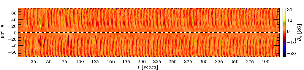
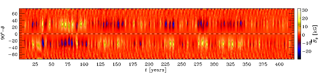
Figure 1: Time evolution of the mean toroidal magnetic field $\overline{B}_{\phi}$ in the convection zone for three depths (from top to bottom, $R_{\rm s}$, $R_{\rm m}$, and $R_{\rm b}$). The extrema are $[-11.0,10.3]$ kG at $R_{\rm s}$, $[-23.3,20.7]$ kG at $R_{\rm m}$, and $[-29.9,31.7]$ kG at $R_{\rm b}$.

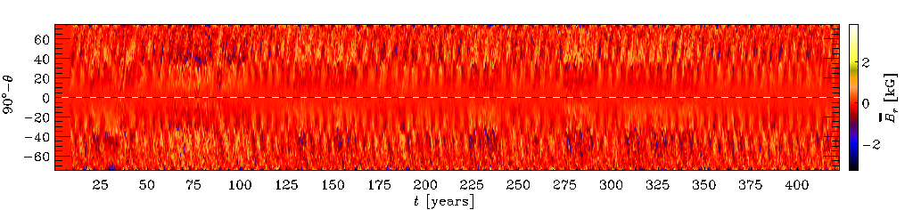
Figure 2: Evolution of the mean radial magnetic field $\overline{B}_{\rm r}$ in the convection zone for three depths (from top to bottom, $R_{\rm s}$, $R_{\rm m}$, and $R_{\rm b}$). The contours have been clipped at half of the maxima/minima, that is $[-11.7,10.4]$ kG at $R_{\rm s}$, $[-6.1,5.7]$ kG at $R_{\rm m}$, and $[-3.3,3.8]$ kG at $R_{\rm b}$, to make the structures elsewhere than at high latitudes visible.

4 Results

We have run our simulation for nearly 430 years in physical time units. The solution we obtain is oscillatory, but it shows very complex behavior. The definition of a mean cycle period is not unique, but, based on the near-surface toroidal magnetic field oscillation, the mean cycle length is, in physical units, 4.9 years, and therefore, on average, our simulation covers 80 cycles. In comparison to the Sun, the obtained cycle length is roughly by a factor of 4 shorter. If, however, this was expressed in solar units, the length of our simulation would roughly correspond to an evolution of two millennia. From a similar simulation with equatorward migrating fields of Warnecke et al. (2015), we find that the cycle length increases with slower rotation, showing that with more realistic parameters it is possible to obtain cycle lengths comparable to the solar value. To evolve a simulation with a longer cycle over the time span presented here, however, is computationally prohibitively expensive. In comparison to EULAG-MHD, the number of cycles covered here is roughly twice as large, and four times larger in comparison to ABMT. Furthermore, more pronounced solar-like latitudinal migration, and irregular behavior are observed in our simulation than in EULAG-MHD. In the ABMT model, a clear solar-like equatorward migration is seen with one MM-type event. Some fundamental differences also relate to the data analysis, especially concerning the EULAG-MHD: In Passos & Charbonneau (2014) the analogue to the sunspot cycle is defined using the toroidal magnetic field strength at the bottom of the convection zone, and a poloidal field proxy is built using the radial field in the near-surface polar regions, while our analysis covers the whole convection zone. Moreover, we restrain ourselves from a detailed comparison to the observed statistical properties of the solar cycle, as we deem such attempts as somewhat pointless due to the vast difference between simulated and real parameter regimes, but concentrate on the general effects that may cause the irregularities that are seen to occur in our simulation.

4.1 Overall evolution of the magnetic field

In Fig. 1 we show longitudinal averages of the toroidal magnetic field as a function of time and latitude (butterfly diagram) for three depths in the convection zone ($R_{\rm s}$, $R_{\rm m}$, and $R_{\rm b}$), and the corresponding plot for the radial field in Fig. 2. The dynamo solution is, in general, very similar to those reported by Käpylä et al. (2012) and Warnecke et al. (2014, 2015) with cyclic behavior consisting of an equatorward-migrating dynamo wave at low latitudes and a polar branch at high latitudes near the surface. The dominating component near the surface is the radial one with roughly twice the strength of the azimuthal component, while the azimuthal field becomes dominant at larger depths, being roughly twice (four) times stronger than the radial field in the middle (at the bottom) of the convection zone, see also Figure 5(e) of Warnecke et al. (2014) for a plot of a similar run. The lack of strong toroidal magnetic field in the top layer is also related to radial field boundary condition at the surface as investigated in details in Warnecke et al. (2015). The marked difference to our earlier results is the irregularity and hemispheric asymmetry seen in the field evolution. During some epochs, the surface activity ceases and/or becomes disturbed (i.e. the cycle length is changing significantly), which can happen asynchronously in different hemispheres. The radial field evolution is more regular than that of the toroidal field, even though the ceased surface activity is perhaps even better seen in the radial field evolution, see Figs. 1 and 2. During the most severe event (20-40 years in the south; 35-45 year in the north), both the radial and toroidal fields near the surface practically vanish. Simultaneously, regions of strong toroidal magnetic field are seen in the near-equator regions (at $R_{\rm s}$), and also in the bottom layers (at $R_{\rm b}$). Even visually, the toroidal field at $R_{\rm b}$ exhibits another toroidal dynamo mode with considerably longer period than the ‘basic’ cycle of 4.9 years seen throughout the simulation. In addition to these dynamo modes, there appears to be a high frequency (short period) poleward dynamo mode in the upper part of the convection zone, confined to the near-equator region, similar as in Käpylä et al. (2012) and Warnecke et al. (2014, 2015). This dynamo mode might be related to a locally operating $\alpha^{2}$ dynamo in the top layers (Käpylä et al. 2013b; Warnecke et al. 2014). The quantitative characterization of these modes is elaborated upon in Sect. 4.3.

The volume- and time-averaged energies of different flow and magnetic field components are listed in Table 2. In Fig. 3(a), we show the volume-averaged rms values of the total and mean magnetic field together with its mean toroidal and poloidal components as functions of time. The dominant component is the fluctuating part containing roughly twice as much energy as the mean field. In a wedge covering only one quarter of the sphere in longitude, the large-scale magnetic field is almost purely axisymmetric and contains only a negligible contribution from non-axisymmetric modes. Of the mean fields, the dominant component is the toroidal one, containing roughly twice the energy of the poloidal component. This is consistent with the conclusion of Warnecke et al. (2014) that the dynamo is of $\alpha\Omega$ type. The poloidal field evolution shows clear cyclicity with modest long-term amplitude variations, whereas the long-term variations of the toroidal field are much stronger. The irregularities are stronger in the early phases of the simulation, the lowered and disturbed surface activity in the butterfly diagrams of Figs. 1 and 2 being clearly seen as a global maximum of the volume-integrated magnetic field energy, especially in the toroidal field, see Fig. 3. The early phases, roughly 3/4 of the simulation length, show markedly irregular behavior, while the latter part, roughly the last 1/4, shows more regular behavior with slightly decreased overall magnetic activity level.

In panels (b) and (c) of Fig. 3, we plot the rms values of toroidal (b) and poloidal (c) components for both hemispheres (north – blue; south – red). The solid black lines in these panels show the ratio of northern to southern energy (expected to attain the value of unity if the hemispheres are totally symmetric). Although averaged over the full time series, the asymmetry measure is close to unity for both the toroidal (2.7% dominance of the northern hemisphere) and poloidal components (1.7% for the north), the variance around the mean is significant (around 0.1) for both field components, although the volume-integrated quantities indicate no clear correlation between the asymmetry and extrema in the total energy. We will investigate the north-south-asymmetry in more detail in Sect. 4.6.

In Fig. 3(d) we plot the toroidal magnetic field strength near the surface (at $R_{\rm s}$, red line) and the bottom (at $R_{\rm b}$, blue line). Roughly thrice stronger toroidal fields are located at the bottom of the convection zone in comparison to the surface. The surface field shows some variability, but significantly smaller than those associated with the bottom toroidal magnetic field. While the surface toroidal field strength shows no systematic trend when the early and late parts of the simulation are compared, the bottom field is clearly decaying in strength. Therefore, the overall decrease and change in the magnitude of the irregularities in the total mean field evolution can be attributed to the changes seen in the bottom toroidal field.

Figure 3: (a) Total ($B_{\rm tot}^{\rm rms}$ (purple dashed), total mean ($\overline{B}_{\rm tot}^{\rm rms}$, black solid), toroidal ($\overline{B}_{\rm tor}^{\rm rms}$, blue), and poloidal ($\overline{B}_{\rm pol}^{\rm rms}$, red) rms values as functions of time as averages over the whole volume. (b) $\overline{B}_{\rm tor}^{\rm rms}$ in the north (blue) and south (red). The black solid line shows the ratio of the northern to southern energy as function of time, and the orange line the mean of the ratio computed over the whole time span. (c) The same for the poloidal field. (d) The bottom (at $R_{\rm b}$, blue line) and surface (at $R_{\rm s}$, red line) toroidal magnetic field strengths as functions of time The thin orange horizontal lines indicate the mean of the quantities over the whole simulation time. In (a) and (d) thick orange lines show the smoothed curve of the total mean magnetic field (a) and the bottom/surface toroidal magnetic field strength (d). and the yellow horizontal lines the 1.1 and 0.9 times the mean levels, respectively.

Figure 4: (a) The rms value of the mean azimuthal velocity as a function of time together with the average over the whole time series plotted with a black horizontal line. The dashed black line shows the volume-averaged rms value of the fluctuating velocity field, $u_{\rm rms}$. The red colour indicates the times which we label as ‘high’, blue symbols ‘low’, and orange ‘nominal’ activity states according to the strength of the total magnetic field (D1, see Sect. 4.5). (b) The rms value of the total magnetic field as a function of time, the same colour coding of overplotted symbols as in (a). The black horizontal line indicates the mean over the whole time series. (c) The rms value of the meridional velocity as a function of time (black solid line) with the mean over the whole time series (orange horizontal line), and a 4.9-year moving average (thick red solid line). (d) A zoom-in to 50-65 years of evolution of the mean azimuthal velocity (black solid), mean meridional velocity (blue line, multiplied by a factor of 10 to fit in the figure), and the total mean magnetic field strength (red line, scaled to fit the figure).

4.2 Overall evolution of the velocity field

In Fig. 4 we show the rms values of the azimuthal, fluctuating (a) and meridional (c) velocities. The system energetics is dominated by differential rotation, the energy of which comprises roughly 57 percent of the total kinetic energy, being roughly 2.6 times stronger than the total magnetic energy. The energy contained in the meridional flow is negligibly small; in terms of the rms velocities, the meridional flow is roughly 15 times weaker than the azimuthal one. The energy of the fluctuations is roughly 1.3 times weaker than the energy of the axisymmetric part. Evidently, the azimuthal velocity becomes strongly affected by the dynamically significant magnetic field. A strong global magnetic field quenches the azimuthal velocity, while during weaker magnetic field epochs, the average azimuthal velocity is higher, as also indicated by the color coding applied in Fig. 4(a) and (b) for high, low and nominal states defined based on the global magnetic energy level (D1; see Sect. 4.5 for detailed definition). The average meridional flow is an order of magnitude weaker, but shows signs of weak systematic variation when a running average with the mean magnetic cycle length is applied. In Fig. 4(d) we show a zoom-in over a time epoch (50–65 years) during which no significant extrema are seen neither in the total magnetic field strength nor the azimuthal velocity. This figure reveals that both the azimuthal and meridional velocities show a variation over the magnetic cycle, stronger in the former, weaker, yet noticeable in the latter. The azimuthal velocity and magnetic field are phase shifted in such a way that the azimuthal velocity grows when the magnetic field is weak, and decays when it is strong, in broad agreement with Warnecke et al. (2012) and Karak et al. (2015). The meridional velocity shows a similar trend, even though it is much more difficult to detect as the fluctuations dominate the weak signal. Therefore, in terms of the magnetic cycle, the angular velocity variations, often called torsional oscillations, occur with twice the frequency of the magnetic cycle itself (see Fig. 7 and Sect. 4.3 for a more thorough analysis). Our results are in fair agreement with those obtained for the EULAG-MHD and ABMT models during the regular periods of evolution.

In contrast to the magnetic field, the mean velocity field components show only very little hemispherical asymmetry, the evolution of the quantities being virtually identical for both, and are therefore not separated for north and south in Fig. 4. It is evident that the strong, frequently occurring, short-term asymmetries are a property of the magnetic field alone and any asymmetry in the flow is probably caused by the asymmetry in the magnetic field. In the top panel of Fig. 7 we plot the time-latitude diagram of the angular velocity variations at $R_{\rm s}$. From this plot it can be seen that on top of the rather weak, regular oscillation with twice the magnetic cycle frequency, which is evident at all depths, there is a rather strong long-term variation of the angular velocity near the equator in the top layers. The origin of this variation is analyzed in detail in Sect. 4.5.1.

Table 2: Summary of the mode quantities.

No.	Period	Energy fraction				$M^{\rm reg}_{i}$	Eq. sym.
		Tot.	$R_{\rm b}$	$R_{\rm m}$	$R_{\rm s}$
$\overline{B}_{\phi}$
1	0.11	-	-	-	0.13	0	0.01
7	4.8	0.46	0.27	0.55	0.39	0.41	-0.12
8	7.0	0.11	0.16	-	-	0.15	-0.13
9	14	-	0.11	-	-	0.09	-0.18
10	27	-	0.12	-	-	0.18	-0.38
11	53	-	0.11	-	-	0.35	-0.36
$\overline{B}_{r}$
1	0.11	-	0.17	-	-	0	0
7	5.0	0.62	0.29	0.60	0.70	0.75	-0.10
11	52	-	-	-	-	0.28	-0.36
$\overline{B}_{\theta}$
1	0.11	-	-	-	0.25	0	-0.01
7	5.0	0.68	0.44	0.75	0.32	0.74	-0.10
8	7.4	-	0.11	-	-	0.14	-0.15
11	62	-	-	-	-	0.37	-0.58
$\overline{u}_{\phi}$
6	2.2	0.19	0.25	0.21	0.17	0.03	0.78
7	3.7	0.14	0.11	0.13	0.15	0.04	0.75
8	7.2	0.14	-	0.13	0.14	0.09	0.73
9	14	0.11	-	-	0.12	0.15	0.70
10	26	-	-	-	0.11	0.28	0.74
11	48	-	-	-	-	0.36	0.64
$\overline{u}_{r}$
1	0.10	0.61	0.60	0.60	0.62	0.06	0.01
2	0.19	0.15	0.15	0.15	0.15	0.03	0.02
11	41	-	-	-	-	0.23	0.23
$\overline{u}_{\theta}$
1	0.10	0.59	0.60	0.58	0.57	0.03	-0.05
2	0.19	0.14	0.14	0.13	0.14	0.01	0
11	43	-	-	-	-	0.29	0.21
$H_{\rm kin}$
1	0.10	0.57	0.54	0.56	0.57	0.02	-0.27
2	0.19	0.13	0.16	0.13	0.14	0.01	-0.22
11	41	-	-	-	-	0.38	-0.48

4.3 Multiple dynamo modes and their significance

The results presented in this section have been obtained by applying EEMD (see App. A) analysis on the azimuthally averaged quantities using an ensemble size of 100 and Gaussian white noise with standard deviation equal to that of the time series being analyzed. The time series were chosen by sampling the simulation domain in radial direction with 12 and in latitudinal direction with 18 points. Our analysis is focused on the components of mean magnetic field, mean velocity field and kinetic helicity, aiming to extract the most significant modes for the given time series globally as well as at three depths ($R_{\rm b}$, $R_{\rm m}$, and $R_{\rm s}$). We also use the $D^{2}$ statistic (see App. B) on some selected data sets to validate the EEMD results, but also to investigate the coherence of the cycles over time.

We detected on average a total number of 13 modes. As expected, it turned out that most of the energy was contained only in a limited number of modes. In the following we use a mode numbering scheme such that the modes are ordered by their average frequency from higher to lower values (the highest frequency mode thus having an index 1). To express the energy contained in each mode quantitatively we will use the notion defined as follows:

$$E_{i}=\frac{\iint(\overline{A_{i}^{2}})ds}{\iint(\sum\limits_{i}\overline{A_{i}^{2}})ds},$$ (3)

where $A$ is the physical quantity analyzed, $i$ is the mode index, $\overline{A_{i}^{2}}$ is the mean square amplitude of the mode, and summation is performed over all modes and integration either over latitude at selected radii or over the full meridional plane.

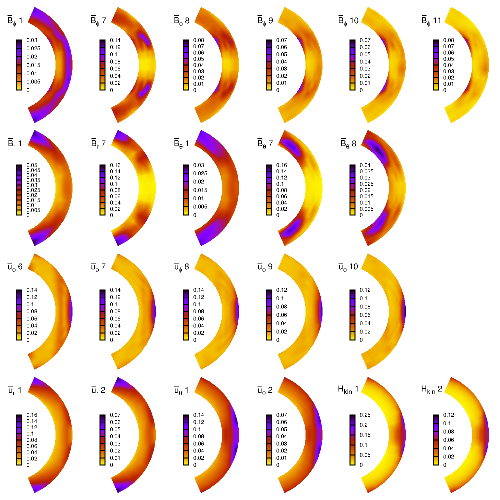
Figure 5: Distribution of mean amplitudes of the most significant modes of mean magnetic and mean velocity fields found from EEMD. The figures are labeled by the physical variable followed by mode index (e.g $\overline{B}_{\theta}$ 7 indicates mode 7 of the mean latitudinal magnetic field). Colors reflect the mean amplitude (blue – high, yellow – low) of the mode at the given location (we note that the scales of separate figures are different). Contours on the plot represent the lines of constant amplitude with values given in the legend.

Figure 6: Phase dispersion analysis results for the components of $\overline{\bm{B}}$. The calculations were done for $\overline{\bm{B}}_{\phi}$ at latitude $\pm 22^{\circ}$ and radius $0.94R_{\odot}$, for $\overline{\bm{B}}_{r}$ at latitude $\pm 66^{\circ}$ and radius $0.94R_{\odot}$ and for $\overline{\bm{B}}_{\theta}$ at latitude $\pm 49^{\circ}$ and radius $0.82R_{\odot}$. Left (right) refers to the northern (southern) hemisphere.

However, calculating only the energy content does not allow us to detect weak, but more regular (harmonic) modes. For that purpose, for each mode we calculate the spectral entropy $H=\int p(\nu)\log p(\nu)d\nu$, where $p(\nu)$ is the power spectral density at frequency $\nu$. Average value of the given quantity per each mode compared to the expected value in the case of white noise serves as a regularity measure of the mode (i.e. how much more Gaussian or non-uniform the spectrum is compared to the spectrum of the white noise). An alternative, but more straightforwardly calculated measure is the ratio of energies in each mode to the expected ones of white noise. A large value of this ratio for a given mode is another indication of the presence of a more regular signal. This idea is captured by the following formula:

$$M^{\rm reg}_{i}=\frac{E_{i}/E^{\rm WN}_{i}}{\sum\limits_{i}E_{i}/E^{\rm WN}_{i}},$$ (4)

where $E_{i}$ is a mode energy fraction defined in Eq. (3) and $E^{\rm WN}_{i}$ is the expected energy fraction of white noise for the given mode. As will be explained later, the results for both regularity measures are in good agreement with each other. For that reason we only show in the following quantitative values calculated based on the second definition.

The results of the EEMD analysis are gathered in Table 3, where the mode period represents a descriptive period which is calculated based on the zero-crossings of the most dominant instance of the mode of given order (i.e. the intrinsic mode function, hereafter IMF, with the highest average mean energy over the full meridional plane). In the table we also show fractions $E_{i}$ of the energy contained in the $i$th mode calculated over the full meridional plane as well as over the latitude at radii $R_{\rm b}$, $R_{\rm m}$ and $R_{\rm s}$. The latter values are approximately equal to the reconstruction error of the initial signal given that the $i$th mode would be omitted from the sum. For clarity reasons only the values above 10% are shown, lower values have been marked with “-”. $i$th mode would be omitted from the sum. For clarity reasons only the values above 10% are shown, lower values have been marked with ”-”. We can see that in the case of the magnetic field components most of the energy is contained in mode 7 (hereafter M7), which can be associated with the dominant cyclicity of 4.9 years cycle length deduced from $D^{2}$ statistic using surface toroidal field. Only for $\overline{B}_{\phi}$ in the bottom layer the energy is more spread between modes with a longer period. From Fig. 5, two upper rows showing the spatial distribution of the mean amplitudes of the most significant modes found in the magnetic field, it is clear that for the toroidal component of the magnetic field, M7 is mainly confined to the region where the equatorward migration of the field is observed (compare Fig. 5, second panel from left in the upper row with Fig. 12, top panel). For the poloidal field, however, the M7 amplitude is the highest at higher latitudes: for the radial field near the surface close to the latitudinal boundaries, and for the latitudinal field, near the bottom and high latitudes. The modes with shorter cycles (mode 1 being the one containing most of the energy, hereafter M1) have the highest amplitudes near the equatorial region and near the latitudinal boundaries, both regions being concentrated near the surface. The long modes (the most notable being mode 11, also having an increased regularity measure, hereafter M11) reside at the very bottom of the convection zone, confined mainly to low-latitude regions.

In the case of $\overline{u}_{\phi}$, the energy spectrum is more flat with roughly equal distribution of energy between modes 6–10. From Fig. 5, third row, it is evident that the highest amplitudes of these modes all occur in the equatorial region, the region extending to higher latitudes for modes 6–7, and getting narrower for the ones with a longer cycle. For the other velocity components as well as for kinetic helicity, defined as $H_{\rm kin}=\overline{{\bm{\omega}}^{\prime}\cdot{\bm{u}}^{\prime}}$, where ${\bm{\omega}}^{\prime}=\mbox{\boldmath$\nabla$}{}\times{\bm{u}}^{\prime}$, energy is primarily contained only in modes 1 and 2. From Fig. 5, last row, we can see that these short cycles are most prominent near the surface close to the latitudinal boundaries for the radial component of the velocity, and near the equator at the surface for the latitudinal velocity component. The modes in the kinetic helicity show high amplitudes near the equatorial region extending deeper to the convection zone, but also in a narrow band near the surface extending the whole latitudinal extent.

In the penultimate column of Table 3, we show a measure of mode regularity as defined in Eq. (4). These values are calculated at those radii and latitudes where the energy of the given mode has its maximum. Higher values of this number indicate higher energy content in the given mode compared to the white noise level. According to the values shown, besides M7 of the magnetic field, we have one additional mode where the regularity has clearly a high value. This is M11, which, however, has a significant energy fraction only in the case of $\overline{B}_{\phi}$ in the bottom layer. It is also quite obvious that the leading modes of $\overline{u}_{r}$, $\overline{u}_{\theta}$, and $H_{\rm kin}$ represent primarily noise, because the value of regularity in these cases is very low. It is noteworthy, however, that for all these quantities the regularity measure of M11 is high, indicating the presence of a long-term regular cycle. Here we also note that the mean spectral entropy calculations lead to similar results as above: the spectrum of M7 of the magnetic field is the most regular one, while modes 10 and 11 are less regular, although significant deviations from the entropy of the white noise spectrum are still detected. It can be concluded, therefore, that the dynamo mode at the bottom of the convection zone has an influence on the overall dynamics of the system despite it being rather insignificant in terms of the total energetics of the system.

The last column of Table 3 represents the equatorial symmetry of the modes, calculated as a time averaged parity defined by Eq. (13). The EEMD analysis confirms our earlier conclusion that the mean azimuthal velocity field is mostly symmetric between the hemispheres, as the parity is high. For all the magnetic field modes, however, values significantly deviating from perfect anti-symmetry (parity values of $-1$) or perfect symmetry (parity values of $+1$) are found. The higher frequency modes show parity values fluctuating around zero, while the lower frequency modes show increasing tendency for antisymmetric parity as the period of the cycle increases. The equatorial symmetry will be discussed in more detail in Sect. 4.6.

As an independent check for the EEMD results we choose the $D^{2}$ phase dispersion statistic (see App. B). Based on the spatial distribution of the most significant modes, we calculate the $D^{2}$ spectra at selected depths for the components of $\overline{\bm{B}}$. Ideally, we would expect to see a match between the average mode periods found from EEMD and cycle lengths found from $D^{2}$.

To focus on the most pronounced activity regions we chose the latitude $\pm 22^{\circ}$ in the layer at $R_{\rm s}$ for $\overline{B}_{\phi}$, latitude $\pm 66^{\circ}$ in the layer at $R_{\rm s}$ for $\overline{B}_{r}$, and latitude $\pm 49^{\circ}$ in the layer at $R_{\rm m}$ for $\overline{B}_{\theta}$ for detecting the short cycles such as M7, see Table 3. Due to the limited length of the data set, the $D^{2}$ analysis is not feasible for detecting the long cycle. However, by using low-pass filtering on the raw data, the existence of M11 can be easily confirmed. The results of the $D^{2}$ analysis are depicted in Fig. 6. Evidence of M7 with a cycle length of around 5 years can be seen for all components. It is interesting, however, that the cycle is modulated differently for northern and southern hemispheres. For the southern hemisphere there is an indication of amplitude modulation with a long period, while for the northern hemisphere the modulation seems to be more complex. If we assume a simple amplitude modulation for the southern hemisphere, and this is justified by the fact that we see a relatively symmetric split of the spectrum when moving from short coherence times to longer ones, then by measuring the difference of these peaks from the spectrum taken at the high end of the coherence time, we can estimate the period of this modulation. Given the low precision that we can achieve using this simple procedure we obtained the value for the modulating period to be around 100$\pm$10 years.

We also analyzed the higher frequency region (0.1 to 2 years) with the $D^{2}$ statistic, but did not detect any strong and/or singular minima in this range. Taken that the regularity measures obtained from EEMD also indicate very low values for these modes, we have to conclude that this cyclic mode is coherent only over very short time intervals, the variation of the length of this cycle being comparable to the length of the cycle itself. Therefore, the signal of this cycle can be spread between multiple EEMD modes, and the spectrum smeared out over a large frequency band.

4.4 Definition of the activity levels

As was evident from the results presented in Sect. 4.1, a decreased surface magnetic activity does not straightforwardly imply a global magnetic energy minimum, especially during those epochs when the long-period dynamo mode at the bottom of the convection zone is strong (roughly speaking the first 3/4 of the simulation). Therefore, the definition of a low/high state is not obvious. Here we use three different definitions, all based on computing running averages with a window coinciding with the main periodicity present at different depths and latitudes (4.9 years):

• If the volume-averaged mean magnetic energy is larger/smaller than the variation of its smoothed average, the state is termed high/low. All other epochs are termed nominal states of activity.

• Otherwise identical, but the surface magnetic field energy at $R_{\rm s}$ in comparison to its smoothed value is used as criterion.

• Otherwise identical, but the energy contained in the magnetic field mode of the bottom layer at $R_{\rm b}$ is used as criterion.

In Fig. 3(a; D1) and (d; D2 and D3) we demonstrate these criteria by overplotting the smoothed curves (orange thick lines) and the corresponding upper/lower limits (yellow horizontal lines) on top of the original data. In the remaining parts of this section, we use these definitions to analyze some key quantities during the different activity states. In practise this is done such that we compute the mean of a quantity over the whole simulation run, divide the data points into different states according to each criterion, and compute the mean profiles for the three activity states separately. If the so-obtained profiles differ significantly from the global mean, i.e. the difference is larger than the standard deviation of the quantity, we take a note of this dependence.

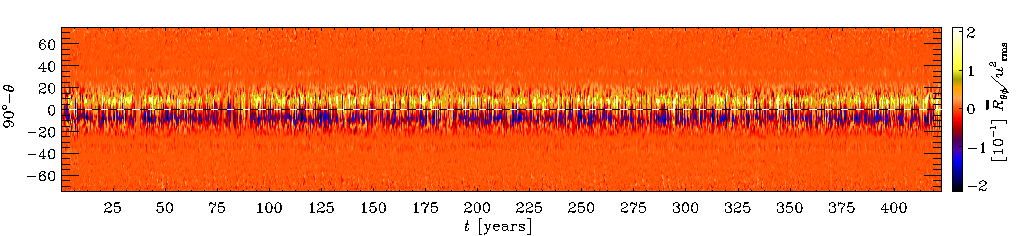
Figure 7: From top to bottom: Time-latitude diagram of the angular velocity variations $\Omega^{\rm v}$, variations of the large-scale Lorentz force $\overline{\bm{J}}\times\overline{\bm{B}}$, and the Reynolds stress components $R_{r\phi}$ and $R_{\theta\phi}$ near the surface (at $R_{\rm s}$). For the Reynolds stress plots, the contours have been clipped at half of the maxima/minima.

4.5 Variation of the dynamo numbers

In this section, we investigate the variability of the three key factors involved in the dynamo process, namely differential rotation and meridional circulation (Sect. 4.5.1), as well as the inductive effects due to convective turbulence ($\alpha$ effect; through kinetic and magnetic helicities as its proxy, Sect. 4.5.2), using the different definitions of the activity level.

4.5.1 Rotation and its non-uniformities

As stated in the Sect. 2, the input angular rotation velocity is five times the solar rotation rate. The differential rotation profile generated in the simulation is solar-like, although the equator is rotating only approximately 7% faster than the poles when the magnetic fields have grown and saturated at dynamically significant strengths. Therefore, the obtained latitudinal differential rotation is approximately three times weaker than in the Sun. We have also performed a hydrodynamical counterpart simulation, in which roughly twice stronger latitudinal differential rotation (pole-equator difference of 14%) is generated. The distribution of angular velocity is fairly similar to the MHD state, discussed later in this section, and therefore the HD results are not shown separately. Furthermore, the hydrodynamic state is steady, and shows no oscillatory behavior similar to the dynamo run. Therefore, the variations seen in the MHD state (Fig. 4) arise as a consequence of the dynamically significant magnetic field to the flow field. Such a backreaction can occur through two pathways: a large-scale Lorentz-force $\overline{\bm{J}}\times\overline{\bm{B}}$ (the so-called Malkus-Proctor effect; see Malkus & Proctor 1975) or through turbulence effects either directly on the convective motions and thereby the generators of differential rotation (the $\Lambda$-effect: see Rüdiger 1989) as recently explored in Karak et al. (2015), or through the turbulent Maxwell stress (e.g. Käpylä et al. 2004). At the same time as quenching the flow field, the magnetic field suppresses its own generators. One argument to explain both the regular and irregular parts of the solar cycle is related to this mechanism (see e.g. ABMT). The classical theory of turbulent hydromagnetic dynamos, however, allows for the excitation of oscillatory solutions independent of the pre-existence of such modulation in the flow field (see e.g. Parker 1955). In this section we set out to investigate the role of the changes seen in the mean flow to the long-term evolution of the magnetic field, especially to its disturbed states.

We begin by investigating the angular velocity variations $\Omega^{\rm v}$ over time in more detail. Here $\Omega^{\rm v}=\Omega-\langle\Omega\rangle_{t}$, where $\Omega=\overline{u}_{\phi}/r\sin\theta+\Omega_{0}$ and $\langle\Omega\rangle_{t}$ is time-averaged over the saturated stage. We plot a time-latitude diagram of this quantity at $R_{\rm s}$ (Fig. 7, top panel), at which depth the most prominent variations occur in the equatorial regions. In addition to the strongest, seemingly irregular, changes symmetrically distributed around the equator, a weaker modulation corresponding to the poleward migrating magnetic cycle can be seen at high latitudes throughout the simulation. In Fig. 7, second panel, we investigate the role of the large-scale Lorentz force $\overline{\bm{J}}\times\overline{\bm{B}}$ in causing the changes seen in the angular velocity. It is evident that the high-latitude variations in the angular velocity, following the mean magnetic cycle, are mediated through this effect. The sudden drops of the surface magnetic field strength are very clearly seen as similar behavior in the large-scale Lorentz force, and occur simultaneously in time in comparison to the surface field disappearances, especially pronounced during the first 50 years of the simulation. Only very mild enhancements of differential rotation at higher latitudes are accompanied by the sudden drops in the Lorentz force. The strong variations seen in the angular velocity near the equator, on the other hand, cannot be explained by the large-scale Lorentz force.

Their symmetric character with respect to the equator hints towards them being related to the Reynolds stress component $R_{r\phi}=\overline{u^{\prime}_{r}u^{\prime}_{\phi}}$. Instead of inspecting all the Reynolds stress components, we concentrate here on examining the variability of those known to be the most significant for the generation of differential rotation, namely $R_{r\phi}$ for vertical and $R_{\theta\phi}=\overline{u^{\prime}_{\theta}u^{\prime}_{\phi}}$ for horizontal differential rotation, and postpone the full analysis of the turbulent quantities to a forthcoming paper (hereafter Paper II). The time-latitude plot of the aforementioned Reynolds stress components are shown in the two lowermost panels of Fig. 7. As is evident from these figures, both stress components undergo variations on the time scale of the shortest dynamo cycle (M1), while showing no modulation by the dominant magnetic cycle (M7). The stresses have non-zero values only near the equatorial regions, where the strongest angular velocity variations are seen. The minima/maxima of the stresses coincide very well with the minima/maxima of the angular velocity and therefore indicate a strong connection between these quantities.

Next we apply the three different definitions of high and low magnetic activity states (D1–D3) introduced above, and seek for significant deviations, indicative of the sensitivity of the mean flow field on the quantity chosen. The mean flow is almost completely insensitive to the variations of the surface magnetic activity level (D2), and not significantly different when the bottom activity level is used (D3). Some significant differences, however, can be detected using the global magnetic activity level (D1) as an indicator.

Results with D1 are depicted in Fig. 8, where we compare the time-averaged rotation profile to the different activity states (low, nominal, and high) denoted and defined as

$$\Delta\Omega_{\rm state}=(\langle\Omega\rangle_{t}-\langle\Omega\rangle_{\rm state})/\Omega_{0},$$ (5)

where $\langle\Omega\rangle_{t}$ is the time-averaged rotation profile, computed over the whole simulation excluding only the initial kinematic stage when the magnetic field is still growing, and the quantities including angular brackets denote averages over a certain state. Using this definition, enhancement/quenching with respect to the average value during a certain state will show up as negative/positive values in the plot, respectively.

The time-averaged rotation profile is very similar to the ones obtained and reported in various earlier works (Käpylä et al. 2012, 2013b), being solar-like, but with a somewhat more cylindrical profile, showing a mid-latitude region of slower rotation leading to a region of reversed sign of radial and latitudinal differential rotation. This region was found to be instrumental in causing the equatorward migration of the magnetic field in Warnecke et al. (2014). The variations in the rotation profile averaged over different global magnetic activity states are weak (roughly 0.4 percent), while the instantaneous variations near the surface (see Fig. 7) could be as large as 5 percent during the early stages of the simulation. During a low/high state, slightly faster/slower equatorial rotation is obtained. This is consistent with the picture that the stronger the magnetic field, the stronger the suppression of the velocity field. The region with a reversed gradient of $\Omega$, however, is observed to persist during all activity states, with virtually no change in its magnitude.

In Fig. 8 (middle row, radial differential rotation; lower row, latitudinal differential rotation) we investigate how the magnitude and distribution of differential rotation change depending on the global magnetic activity level. Here we define the radial shear as $\Delta_{r}=\partial\Omega/\partial r$ and the latitudinal shear as $\Delta_{\theta}=\partial\Omega/r\partial\theta$, and the profiles computed over difference activity states as

$$\Delta_{i,\rm state}=\langle\Delta_{i}\rangle_{t}-\langle\Delta\rangle_{i,\rm state},$$ (6)

where the quantities with angular brackets are averages over the whole time series except for the kinematic stage (index $t$) or over a certain state (index $i$). It is evident that during high/low states of magnetic activity, also the radial differential rotation is quenched/enhanced similar to the rotation itself, the magnitude of the change being roughly 1.5 percent in the equatorial region. No significant change is seen for the latitudinal differential rotation, except for at the high latitude regions, which show hemispheric asymmetry especially during the low state. Finally, we define a dynamo number describing the magnitude of the radial differential rotation as

$$C_{\rm\Omega}=\frac{\Delta_{r}(\Delta r)^{3}}{\eta_{\rm t0}},$$ (7)

where the turbulent diffusivity is approximated by $\eta_{\rm t0}=\tau u^{\prime\,2}_{\rm rms}(r,\theta)/3$, with $\tau=\alpha_{\rm MLT}H_{p}/u^{\prime}_{\rm rms}(r,\theta)$ being the local turbulent correlation time, $\alpha_{\rm MLT}$ the mixing length parameter and $H_{p}=-(\partial\ln p(r,\theta)/\partial r)^{-1}$ the pressure scale height. Following our previous studies, we use $\alpha_{\rm MLT}=5/3$. The spatial distribution of $C_{\rm\Omega}$ follows closely that of the radial gradient of the angular velocity (the leftmost panel in the middle row of Fig. 8), and therefore we do not separately plot it, while merely report its spatial extrema $[-30,110]$ averaged over the whole time span of the simulation, which is similar to those obtained in Käpylä et al. (2013b) and Warnecke et al. (2014).

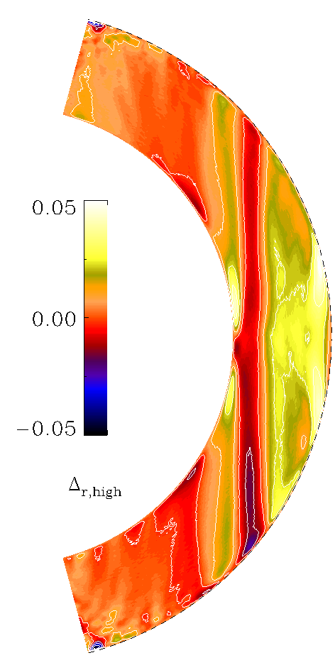
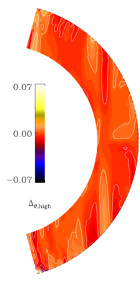
Figure 8: Top row, from left to right: normalized time-averaged rotation profile $\langle\Omega\rangle_{t}/\Omega_{0}$, difference to the rotation profile, $\Delta\Omega_{\rm state}$, during the high, low, and nominal state of global activity (D1). Middle (bottom) row, the same for mean radial (latitudinal) differential rotation.

Figure 9: Meridional flow, indicated as arrows, and time-averaged dynamo parameter $C_{\rm u}$, indicated with color contours. On the left, we show the meridional circulation profile averaged over the whole simulation time span, and the next three panels show the difference $\Delta C_{\rm u,\langle state\rangle}=C_{\rm u}-C_{\rm u,\langle state\rangle}$ to the mean during a high, low, and nominal global activity state (D1).

Next we examine the meridional flow profiles and compute a dynamo number

$$C_{\rm u}=\frac{\overline{u}_{\rm mer}^{\rm rms}\Delta r}{\eta_{\rm t0}},$$ (8)

where $\overline{u}_{\rm mer}^{\rm rms}=\sqrt{\overline{u_{r}}^{2}+\overline{u}_{\theta}^{2}}$ and other quantities are defined in the same way as in Eq. (7). The largest deviation from the time-averaged profile is, similar to the differential rotation, obtained when the activity states are defined based on the global magnetic field energy (D1), the magnitude of the change being maximally 6 percent in a thin layer concentrated in the equatorial region near the surface. The results are presented in Fig. 9, zoomed into the equatorial region. There are, however, some enhanced meridional flows generated also near the latitudinal boundaries, but as these are most likely artefacts arising from the latitudinal boundaries, they are not shown here. The meridional flow pattern (Fig. 9 leftmost panel) is very similar to those obtained earlier by Käpylä et al. (2012, 2013b) and Warnecke et al. (2013, 2015), i.e. consisting of three cells in radius, aligned with the inner tangent cylinder. Additionally, there is one anti-clockwise cell confined near the surface and equator, the near-surface poleward flow being the strongest at this location. The strongest variations in magnitude over time are related to this region. The dynamo number is varying spatially between 0…3 averaged over the whole simulation time span, the dynamo number of the meridional flow being more than thirty times weaker than of the $\Omega$ effect (radial differential rotation). The high (second panel in Fig. 9) and low (third panel in Fig. 9) states show no marked difference in the spatial distribution nor strength of the main cells, the small near-equator cell undergoing the strongest variations. The most interesting observation is the marked hemispheric asymmetry pronounced especially during the low state: the meridional flow in the southern hemisphere is more strongly quenched than the northern one. Similar, but the effect being more localized to the surface regions, is seen during the high state, when the northern surface flow gets reduced, while the southern one gets stronger.

In conclusion, if the MM was an epoch of a global magnetic energy minimum, our results would predict faster surface rotation, stronger differential rotation, and hemispherically asymmetric meridional flow pattern. If actually a global magnetic energy maximum was occurring in the deeper layers of the convection zone during the MM, then our prediction would be reversed to slower surface rotation and weaker differential rotation, while the meridional flow would retain its asymmetric character. Neither of these scenarios is consistent with the actual observations of sunspot proper motion during the MM (Eddy et al. 1976; Ribes & Nesme-Ribes 1993). Overall, however, our analysis suggests that the surface activity disturbances have no direct and/or straightforward relation to changes in the rotational speed nor the strength of differential rotation. Moreover, the meridional circulation is so weak that it is most likely incapable of influencing the global dynamics significantly. During the first 100 years of the simulation there are strong dips in the angular velocity, accompanied by simultaneous maxima in the global magnetic field strength. Only one of these events (during $t=20$–$45\,{\rm yrs}$), however, leads to the disappearance of the surface activity. Even then, the dip in the angular velocity does not coincide with the beginning and the duration of the disturbed surface activity period. Therefore we can conclude that the surface irregularities do not originate from the variations seen in the angular velocity or meridional circulation, at the same time noting that a disturbed surface activity may not be indicative of a decrease in the global magnetic energy level.

4.5.2 Proxy of the $\alpha$ effect

We build a proxy for the isotropic $\alpha$ effect following the definition of Pouquet et al. (1976),

$$\alpha=-{\textstyle{1\over 3}}\tau(\overline{\mbox{\boldmath$\omega^{\prime}$}\cdot{\bm{u}^{\prime}}}-\overline{{\bm{J}}^{\prime}\cdot{\bm{B}}^{\prime}}/\overline{\rho}),$$ (9)

where the current helicity consists of the fluctuating current ${\bm{J}}^{\prime}=\mbox{\boldmath$\nabla$}{}\times{\bm{B}}^{\prime}/\mu_{0}$ and the fluctuating magnetic field ${\bm{B}}^{\prime}={\bm{B}}-\overline{\bm{B}}$. When looking at the kinetic and magnetic contributions to the $\alpha$ effect proxy, it can be observed that the kinetic helicity is dominating the signal, the current helicity being roughly an order of magnitude weaker. Therefore, we mostly concentrate in the following on examining the properties of the kinetic helicity, while also computing a suitable dynamo number.

First we examine the time evolution of the azimuthally averaged kinetic helicity $H_{\rm kin}=\overline{\mbox{\boldmath$\omega^{\prime}$}\cdot{\bm{u}^{\prime}}}$. This quantity shows a clear mean signal as a function of latitude, so that negative (positive) values are obtained in the north (south), increasing towards the poles where maximal values are obtained, with a strong localized enhancement seen in both hemispheres in the low-latitude regions, extending at least half of the depth of the convection zone. Close to the bottom of the convection zone at high-latitude regions, the sign of this quantity is reversed. These results are in agreement with earlier ones both in local and global domains (e.g. Käpylä et al. 2009, 2013b). In Fig. 10(a), we show this quantity with the mean profile over the whole time series subtracted, showing that most of the variation occurs near the equatorial region. The signal is dominated by the high-frequency modes (M1 and M2), while at higher latitudes the dominant mode M7 in the magnetic field is detectable, but not significant in comparison to the high-frequency signal. The zoomed-in plots of Fig. 10(b) and (c) reveal the presence of the weak basic cycle modulation in the kinetic helicity, but with half of the length of the magnetic cycle. Especially during times of clear antisymmetry, Fig. 10(d), a modulation pattern is seen near the surface both at low latitudes (location of the strongest signal in kinetic helicity, shown with solid lines in the figure), and at higher latitudes (location of the toroidal magnetic field maximum; dashed lines). The modulation pattern is such that the extrema of helicity roughly coincide with those of the radial magnetic field at mid-latitudes (shown with dotted lines in the figure). During times when M7 shows stronger symmetry with respect to the equator, Fig. 10(e), all the observed weak dependencies in the earlier antisymmetric phase of the simulation break down, although signs of immediate restoration of the modulation pattern can be detected when the symmetry abruptly switches at around $t=234\,{\rm yrs}$ back to antisymmetric one. Interestingly, signs of a longer-term modulation are seen in Fig. 10(d), as during that epoch the kinetic helicity signal is systematically more negative (positive) in the north (south) in comparison to the mean value over the whole time span. This is also manifested in Fig. 10(b) as persistent blue (yellow) stripes at low northern (southern) latitudes. Detected by EEMD only through the high value of the regularity measure, however, this modulation is of very low energy in comparison to the high-frequency modes.

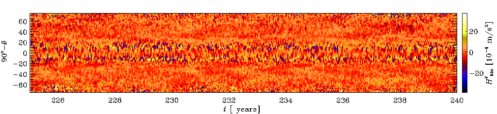
Figure 10: (a) Time-latitude plot of the kinetic helicity variations $H_{\rm kin}^{\rm v}=H_{\rm kin}-\langle H_{\rm kin}\rangle_{t}$. Zoomed-in plots of $H_{\rm kin}^{\rm v}$ over $t=50$–$65\,{\rm yrs}$ (b) and $t=225$–$240\,{\rm yrs}$ (c). (d) $H_{\rm kin}$ at $\pm 10^{\circ}$ (solid) and $\pm 25^{\circ}$ (dashed) latitude for north (blue) and south (red) with the means over the whole time series indicated with an orange horizontal lines. The data is averaged with a running mean over a 1-year window, to smooth out the dominant high-frequency component. The dotted lines show the radial magnetic field at $\pm 25^{\circ}$ latitude, scaled to fit the plot. All quantities are plotted at $R_{\rm s}$.

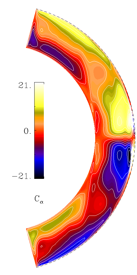
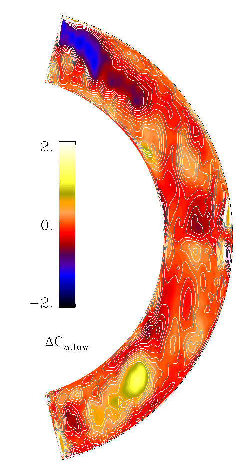
Figure 11: From left to right: $C_{\alpha}$ time-averaged over saturated stage. Difference to the $C_{\alpha}$ profile during the high, low, and nominal state of surface magnetic activity (D2).

Next, we define and compute a dynamo number

$$C_{\alpha}=\frac{\alpha\Delta r}{\eta_{\rm t0}}.$$ (10)

This quantity is plotted in Fig. 11, left panel, as the time average over the whole length of the simulation. The profile is similar to those obtained earlier, e.g. in Runs C1 and C2 of Käpylä et al. (2013b).

This dynamo number is almost an order of magnitude larger than the corresponding one from meridional circulation, but roughly 5 times weaker than the one estimated from radial differential rotation. The strongest deviation from the mean profile is obtained when high and low states are determined according to the surface activity level (D2), while selecting the time points based on the global (D1) and bottom energy (D3) levels produce no significant deviation from the mean. During the low state, the $\alpha$ effect is strongly enhanced i.e. significantly larger positive/negative values are obtained in these regions in north and south, respectively. During the high state, there is also a mild enhancement, while in the nominal state the $\alpha$ effect is strongly reduced. The magnitude of the enhancement/quenching is the largest of all the dynamo drivers, roughly by 30 percent, but acts to the opposite direction as expected, i.e. with a locally and temporally larger $C_{\alpha}$, the naive expectation is to obtain a more efficient dynamo near the surface, but weaker surface activity is seen.

We also compute the migration direction of the magnetic field predicted by the Parker-Yoshimura sign rule (Yoshimura 1976)

$$\bm{\xi}_{\rm migr}=-\alpha\hat{\bm{e}}_{\phi}\times\nabla\bm{\Omega},.$$ (11)

We plot this quantity on top of the rms-value of the mean toroidal magnetic field in the convection zone in Fig. 12, top panel. In the entire region of negative radial shear, manifested by the region of slower rotation in the differential rotation profile, equatorward migration is predicted to occur in both hemispheres. This region coincides with a toroidal field belt having a maximum roughly at $\pm 28^{\circ}$ latitude and $0.85\,R_{\odot}$ depth. There is another equatorward migration region at the very bottom of the convection zone, coinciding with the location of the strongest toroidal field belt roughly in a similar latitude range. In the upper third of the convection zone, however, the predicted migration direction is poleward. This matches with a toroidal magnetic field belt at $\pm 22^{\circ}$ latitude and $0.9\,R_{\odot},$ depth. No strong radial migration is predicted for the lower parts of the convection zone, within which both upward and downward regions are seen, but without a clear systematic pattern. The good agreement of the predicted and actual migration direction as well the migration pattern itself fit well with the work of Warnecke et al. (2014, 2015). The migration pattern does not change significantly using any of the activity level definitions (D1–D3), which is likely due to the fact that the gradients of the angular velocity and the kinetic helicity, and therefore the $\alpha$ effect, are sensitive to different activity indicators (the former to the global, the latter to the surface) and the signal is cancelled out. Therefore, we note that the $\alpha$ effect shows the most interesting behavior during the extrema seen in the surface activity, but our approach to investigate its effects via simple scalar proxies of kinetic and magnetic helicities is inadequate; we will return to this problem in Paper II.

Finally, to investigate whether the different lengths of the dynamo solutions and their distinct spatial distribution is due to a systematic, strong dependence of the magnetic diffusivity or magnetic Reynolds number

$${{\rm Re}_{\rm M}}(r,\theta)=\frac{\alpha_{\rm MLT}H_{p}u^{\prime}_{\rm rms}(r,\theta)}{\eta},$$ (12)

where $\eta=10^{8}$ m² s^-1 is the molecular diffusivity, profile either on radius or latitude, we plot their radial profiles at two different latitudes in Fig. 12, lower panel. To explain the co-existence of dynamo solutions with more than two orders of magnitude varying periods between the bottom and the top with the dependence being due to a weaker diffusivity in the bottom parts, a two orders of magnitude increase of the magnetic Reynolds number as function of radius should be seen. Even though the trend seen is indeed increasing as function of depth, the magnitude of the increase is maximally four, being too weak to provide an explanation.

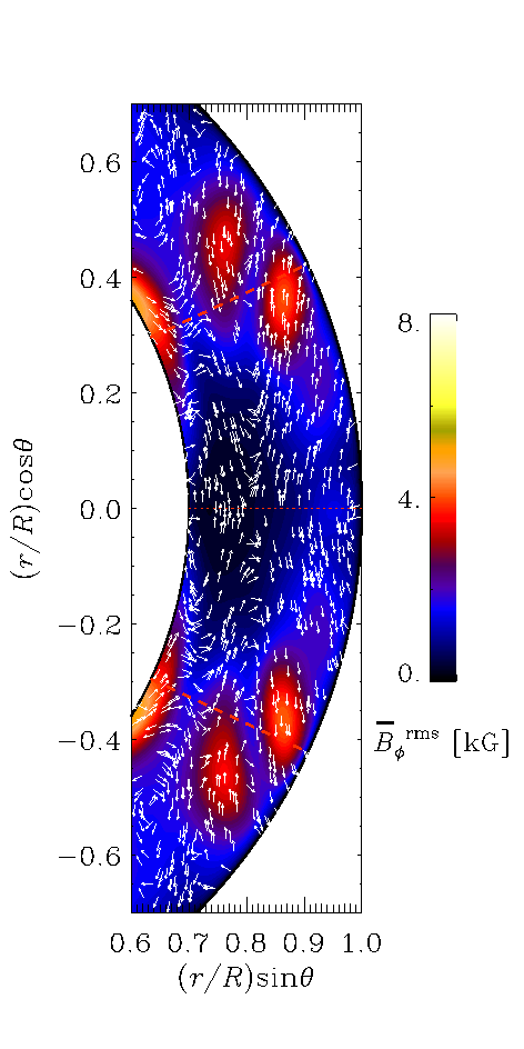
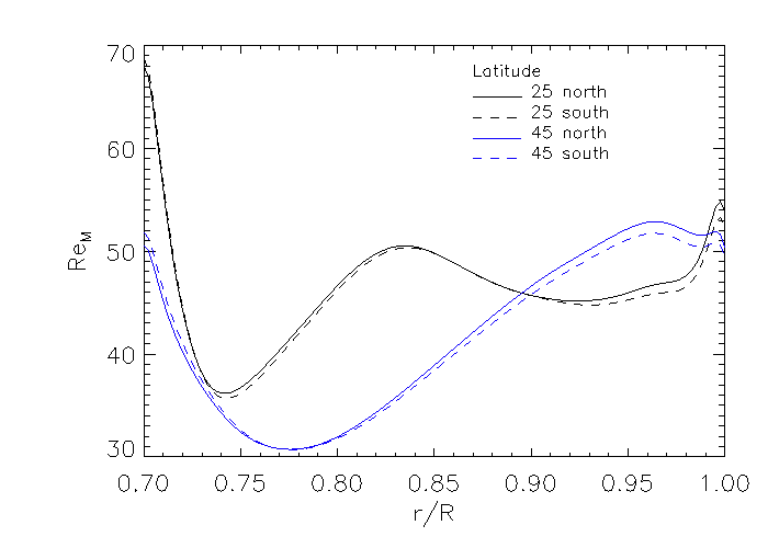
Figure 12: Top panel: color contours of $\overline{\bm{B}}^{\rm rms}_{\phi}$ in kGauss averaged over the whole simulation run, zoomed-in to show the near equatorial region. The overplotted arrows show the predicted (Eq. 11) time-averaged mean migration direction ${\bm{\xi}}_{\rm migr}$ normalized to unity. The dashed red lines show the radius at $\pm 25$ degrees of latitude. Lower panel: radial dependence of the magnetic Reynolds number at two latitudes (north – solid; south – dashed.

4.6 Equatorial symmetry

In Fig. 13 we plot the equatorial symmetry of the magnetic field, defined as

$$P=\frac{E_{\rm even}-E_{\rm odd}}{E_{\rm even}+E_{\rm odd}},$$ (13)

where $E_{\rm even}$ is the energy of the quadrupolar (symmetric) and $E_{\rm odd}$ the energy of the dipolar (antisymmetric) mode of the magnetic field. In Fig. 13(a) we show the global parity as a function of time. This quantity is obtained by computing, for each latitude pair for certain depth, the energies contained in the even and odd modes, and taking the mean of the obtained data. Evidently, the parity is mixed throughout the whole simulation, the dominant mode being the dipolar (solar-like) mode (average parity $-0.15$ over the whole time series). A difference can again be observed between the first 3/4 of the simulation (average parity of $-0.26$) in comparison to the last quarter, when there are larger fluctuations around the clearly positive mean parity of $0.1$.

The best correlation between the different activity level definitions can be obtained when D3 is used. The parity not only shows a clear modulation with a similar long-term cycle as the toroidal field in the bottom of the convection zone, but also a clear pattern is revealed for the first 3/4 of the simulation with the D3 color coding: during a bottom mode minimum, the parity also obtains a minimum ($-0.42$), while during a high state, the parity is the least solar-like ($-0.14$). During the last quarter of the simulation, the bottom mode is so weak, that it falls below the low activity limit for the whole epoch. Nevertheless, the long-term cycle persists both in the bottom mode and in the parity, suggesting a relation between these quantities.

As can be seen from Table 3, the low-frequency bottom mode (M11) is predominantly of dipolar symmetry (mean parity $-0.36$). From Fig. 13(b), it is evident that rather strong parity fluctuations are related to this mode, the excursions to positive parity being more short lived than the periods spent in the negative parity region. The majority of the parity variation, however, is related to the dominant ‘basic’ cycle (M7), which on average has a parity of roughly $-0.12$, but its symmetry is strongly fluctuating as a function of time, as is evident from Fig. 13(b). The parity is fluctuating even more strongly than that of M11, between nearly purely dipolar and quadrupolar states. Most of the time M7 and M11 and in anti-phase, i.e. when M11 attains the largest positive value, M7 is the most negative. There is a tendency for irregular behavior when the parities of these modes are in phase, such as during $t=20$–$45\,{\rm yrs}$ and $t=250$–$300\,{\rm yrs}$. In Fig. 13(c) and (d) we show two zoom-ins of the parity evolution, panel (c) showing a clearly regular, antisymmetric behavior of the system and the surface toroidal field ($t=50--65\,{\rm yrs}$), while panel (d) shows a predominantly symmetric state that during only a half a cycle changes into a antisymmetric one ($t=225$–$235\,{\rm yrs}$). During the former epoch, the bottom toroidal magnetic field strength attains a minimum, while during the latter, a maximum is observed.

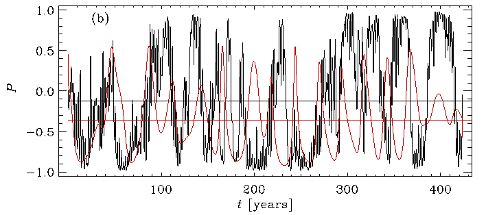
Figure 13: (a) Parity $P$ as function of time. The color coding is defined using Definition D3. (b) Parity of M7 (black) and M11 (red) as function of time; their means are indicated with the horizontal lines with the same color coding. (c) Parity (black) and toroidal magnetic field near the surface (blue: north, red: south) at $\pm 25^{\circ}$ latitude, during the low state of the bottom toroidal mode, panel (d) shows the same quantity, but for a high state of the bottom toroidal mode.

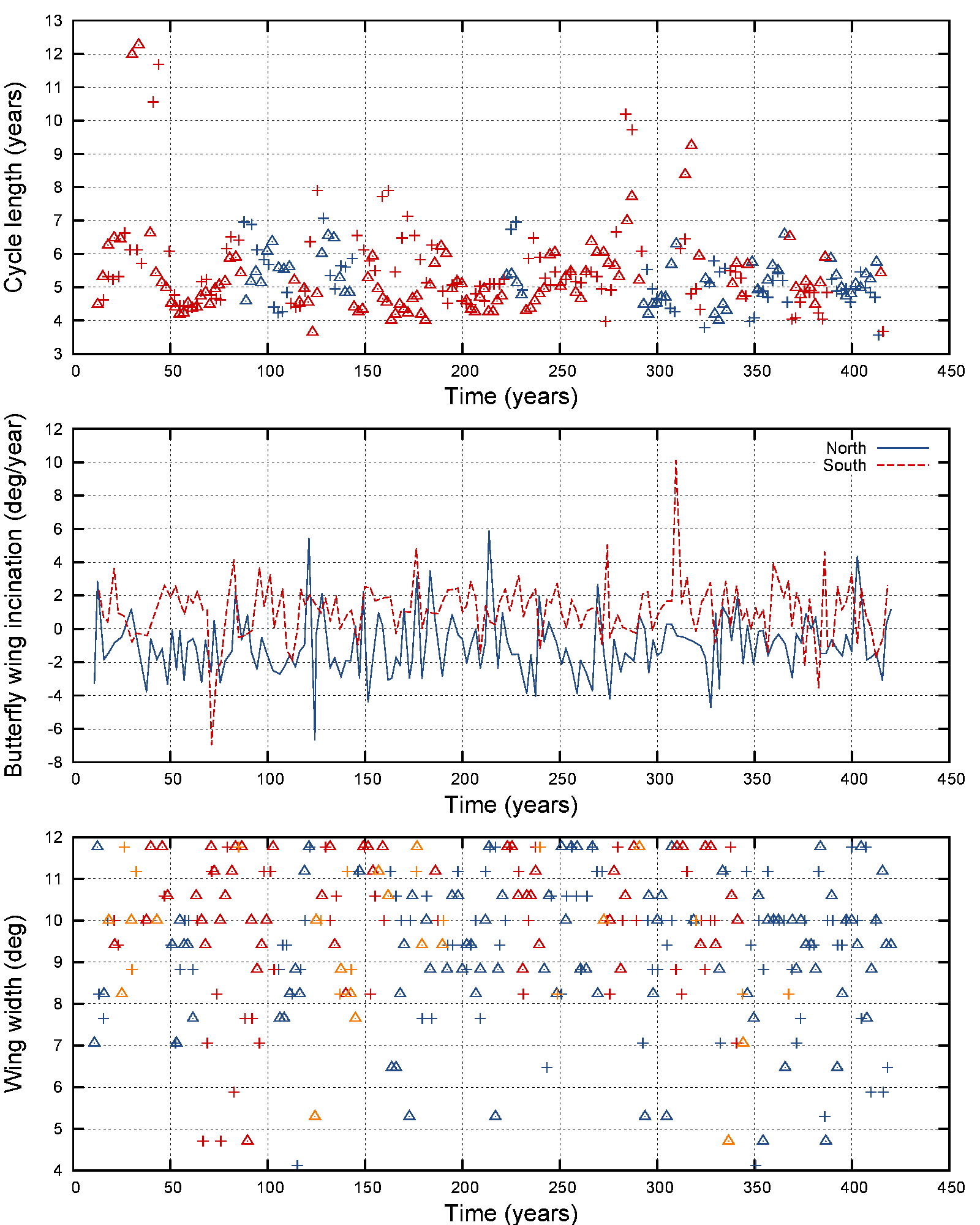
Figure 14: Top panel: magnetic cycle length determined from the toroidal magnetic field, $\overline{B}_{\phi}$, at $\pm 25^{\circ}$ latitude and $r=R_{\rm s}$, blue/red indicating positive/negative parity, north with triangle and south with plus symbols. Middle panel: time evolution of butterfly wing inclination. Bottom panel: butterfly wing widths, red/orange/blue indicating high/nominal/low bottom magnetic field energy (according to D3), north with triangle and south with plus symbols.

4.7 Variation of general cycle properties

Evidently, the overall properties of the magnetic cycles show quite a large variation over time. In Fig. 14 we plot three indicators, namely the cycle length of the toroidal field near the surface at $\pm 25^{\circ}$ latitude, the inclination of the butterfly wing, and the butterfly width in degrees for north (triangle symbols) and south (pluses) separately.

As for the toroidal field cycle length (Fig. 14, top panel), two distinct types of events can be seen: During suppressed magnetic activity near the surface layers ($t=$20–45, 275–285, and 310–320$\,{\rm yrs}$), the field ceases to change its sign; therefore, some cycles are ‘missed’, and then twice as long cycles are detected as a result. The other type of variation are the less abrupt fluctuations around the mean cycle length, the shortest cycle lengths being slightly less than 4 years and the longest one around around 8 years. The cycle length is not sensitive to any of the activity level definitions (D1–D3), but there is a tendency for the cycles to be shorter if the parity is more symmetric (blue symbols), while larger cycle length variations occur for more solar-like (antisymmetric; red symbols) parities. Also, all the ‘missing’ cycles occur during the more solar-like parity, during which the bottom cycle is attaining its minimum.

To further analyze the general cycle properties we have filtered the surface magnetic field data so that only points with $|\overline{B}_{\phi}|>4kG$ have been retained. This way the concentrations of strong magnetic field are clearly grouped into separate half-cycles or wings. The relative properties of these structures, such as the latitudinal extent (width) and duration can then be directly measured. Based on these properties we define the inclination of the butterfly wing as the half cycle width divided by its duration. For north/south, a solar-like cycle would have negative/positive inclinations, while for cycles where migration is weak or non-existent, values close to zero are expected. As is evident from the middle panel of Fig. 14, there is a tendency for the ‘missing’ cycles to appear with weak migration only. Anti-solar cycles are also observed quite a number of times both for north and south, but not at simultaneous epochs. It appears that the shorter the cycle, the higher is the probability for anti-solar migration pattern.

The corresponding butterfly width (Fig. 14 bottom panel) is most often large for the ‘missing’ cycles, which is in striking contrast to the observational evidence for the MM (see Usoskin et al. 2015, and references therein), if these two types of events are in reality representing one and the same phenomenon. There is a tendency for narrow widths to occur when the bottom magnetic field is weak.

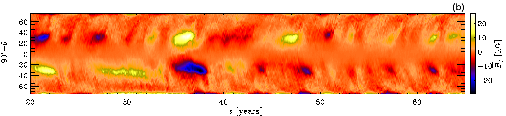
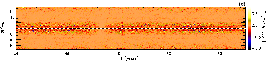
Figure 15: From top to bottom: Zoom-ins of the time-latitude diagram of the mean toroidal magnetic field near the surface (at $R_{\rm s}$) and bottom (at $R_{\rm b}$), the angular velocity variations, and the Reynolds stress components $R_{r\phi}$ and $R_{\theta\phi}$ near the surface (at $R_{\rm s}$) during $t=20$–$65\,{\rm yrs}$, showing that the magnetic cycle and surface activity are strongly disturbed ($t=20$–$45\,{\rm yrs}$), after which the regular state is quickly recovered ($t=45$–$65\,{\rm yrs}$).

4.8 Irregular event during 20–45 years

Finally, we present a close-up of the most clearly pronounced irregular activity epoch during 20–45 years. In Fig. 15, we reproduce the plot shown in Fig. 7, but restrict the plotting range to 20–65 years, which shows both the irregular evolution, followed by the resumption of the regular behavior, indicating that the system changes itself into very abruptly after the distortion. The time resolution in the figure is high enough to clearly show the high-frequency (M1) mode of the magnetic field (top), not well discernible in any other longer time span figure; this cyclicity is seen to persist regardless of the irregularities seen in the modes M7 and M11.

The irregular behavior is first seen in the southern hemisphere, see Fig. 15(a), and the event appears to be preceded by a field enhancement in the bottom mode (M11; Fig. 15(b)). Even though the toroidal field of the mode M7 gets very weak, the surface activity does not totally cease, but the field evolves with significantly longer period without a polarity change. The southern cycle, therefore, appears truly as a ‘missed’ one; meanwhile the northern hemisphere continues as usual. After twice the time of a normal cycle has elapsed, the bottom magnetic field attains another strong maximum. This is reflected by a strong minimum in the Reynolds stresses, Fig. 15(d) and (e), and surface differential rotation, Fig. 15(c). Immediately after this, the toroidal magnetic field practically vanishes from the northern hemisphere, while the south seems totally unaffected by the northern disruption. Again, after the south has produced two normal-looking magnetic cycles, normal activity is rapidly restored also in the north. After that, the bottom magnetic field exhibits no further strong extrema, and the mode M7 continues its evolution in a regular manner. It is also noteworthy that the bottom magnetic field changes its polarity during the disturbed epoch.

During this epoch, it is evident even by eye that there is especially strong equatorial (north-south) asymmetry related to the surface toroidal magnetic field. This is reminiscent of the observations of the Maunder and Dalton minima (Ribes & Nesme-Ribes 1993; Usoskin et al. 2009), that indicate strong hemispheric asymmetry and a relatively strong quadrupolar component of the magnetic field. The global parity does not strongly reflect this local surface anomaly as a sudden, persistent change towards a quadrupolar state (+1), although the quantity fluctuates strongly between the values [-0.9,0.7]. This is most likely due to the fact that the symmetry properties of the very strong bottom toroidal magnetic field dominate the signal, at all times remaining close to a dipolar configuration.

Although similarly dramatic events cannot be isolated from the rest of the time series, it is clear that both extrema and polarity reversals of the bottom mode M11, frequent during the first 3/4 of the simulation time, make the system more irregular than during the last 1/4 during which especially the energy contained in the bottom mode M11 gets weaker.

5 Conclusions

In this paper we have analyzed a semi-global (wedge-shaped) DNS that produces a solar-like oscillatory dynamo with surface migration properties of the magnetic field resembling those from observations. The mean cycle length is 4.9 years, and the simulation is evolved over 80 such magnetic cycles. If scaled to solar units using the fact that the Sun has a magnetic cycle of roughly 22 years, our simulation would correspond to two millennia of solar evolution. The chosen parameters, most notably the modest stratification and the values of the Reynolds numbers, are still far from the real Sun; nevertheless, this combination of parameters produces a solar-like dynamo, and it is computationally affordable to integrate over a large number of cycles. The rotation rate is five times solar, resulting in a roughly three times weaker differential rotation than in the Sun. The rotation profile is solar-like, but somewhat more cylindrical, and the meridional circulation consists of multiple cells in radius. Nevertheless, we can expect that this simulation can well be used to study the long-term evolution of solar-type dynamos.

A general property of the dynamo solution is its cyclic nature: even though there is a clear magnetic cycle, the various nonlinearities in the system drive it away from an exactly periodic (harmonic) state. Therefore, special time series analysis techniques are needed that can cope with non-periodic signals. In this study, we perform a statistical analysis over the whole convection zone, investigating the properties of all relevant quantities at different depths and latitudes. The methods we choose to employ are the EEMD and $D^{2}$ statistics.

The behavior of the dynamo solution is extremely complex. In addition to changing cycle length, we observe epochs of disturbed and even ceased surface activity, and strong short-term hemispherical asymmetries. The major general findings related to the overall dynamics of the system include:

• The hemispheric asymmetries are related to the magnetic field alone, while the velocity field remains almost perfectly symmetric at all times.

• The epochs when the surface activity has decreased or is practically non-existent are not global magnetic energy minima but maxima, as strong magnetic fields are stored in the deeper parts of the convection zone.

The main goal of this study is to find the causes for the irregular behavior rather than to make direct comparisons with the observed characteristics of the solar magnetic cycle. Therefore, we have concentrated our efforts toward analyzing the dynamo solution itself to investigate how the most important properties (cycle length, migration properties, energetics) change during the irregular epochs. We also investigated all the key factors in the dynamo process, namely the rotation and its non-uniformities, meridional circulation, the inductive action arising from turbulent convection ($\alpha$ effect), and the changes of these as functions of a relevant activity level measures. The major findings from this part of the analysis can be summarized as follows:

• The specific dynamo solution analyzed here contains not only one, but three separate modes, having distinct cycle lengths and symmetry properties, and are located in different parts of the convection zone. The dominant mode is the near-surface 4.9 year cycle (denoted with M7) showing equatorward migration at lower latitudes and poleward migration at higher latitudes. This mode is accompanied by a weaker high-frequency poleward migrating mode (M1, 0.11 years) in the equatorial region and a low-frequency mode at the bottom of the convection zone (M11, roughly 50 years).

• The crucial property of the different dynamo modes is their different symmetries. While the dominating surface mode has a mixed equatorial symmetry that undergoes strong fluctuations over time, the bottom mode exhibits nearly pure antisymmetry and is also more regular than the surface mode.

• There is a close relationship between the global magnetic and kinetic energies such that strong magnetic fields quench the flow field in a manner that the angular velocity is significantly reduced, differential rotation gets somewhat weaker, and the meridional circulation attains an asymmetric character with modifications of the circulation magnitude especially in near-equatorial surface regions. We expect that this is what would have been seen during the MM, if it was an event corresponding to the abrupt disappearance of surface activity with a simultaneous global energy maximum in the bottom of the convection zone (see e.g. Küker et al. 1999; Karak 2010, for similar arguments).

• A more common way of interpreting MM is an overall drop of the magnetic activity level. Our simulation produces no such events, which is naturally no proof of them not occurring in the real Sun. The only quantity markedly linked to the surface magnetic activity level in our model is the magnitude of the $\alpha$ effect.

• Two kinds of irregularities are separable from the dynamo solution itself: smooth variations in the cycle properties and abrupt changes that lead to ‘missing’ cycles and ceased surface activity. All these can be satisfactorily explained as the interplay of the different dynamo modes and their influence on the flow field.

Even though this simulation has been run for a considerable length of time, we still observe a secular trend – especially for the long-term cycle in the bottom of the convection zone. To fully capture and understand this trend, and to find out whether it is a transient or a real cycle, the simulation would still need to be continued further. Although we have presented an already rather elaborate and time consuming data analysis of the results, we have merely touched upon the turbulent quantities. Especially the $\alpha$ effect was treated in a very simplified manner, only using a proxy from the kinetic helicity, which is far from adequate. We recently undertook an effort to compute the full tensorial representation of both the diffusive and anti-diffusive contributions to the electromotive force using the spherical test-field method (Warnecke et al. 2016) from a rather similar, but shorter, solar-like dynamo simulation. It would therefore be useful to compute and compare the turbulent transport coefficients from the different epochs of the long run presented here. The simplified analysis presented here, however, re-affirms our earlier conclusion of the general dynamo solution and its migration being explicable in terms of a turbulent $\alpha\Omega$ dynamo (Käpylä et al. 2012; Warnecke et al. 2014).

Appendix A Empirical Mode Decomposition

Fourier spectral analysis provides a general method for examining the global energy–frequency distributions. For its validity, some crucial conditions must hold: the system must be linear and the data must be strictly periodic or stationary. If these restrictions are not satisfied, the non-stationary nature of the data causes the energy to be spread over a wide frequency range. Additionally, deformed wave-profiles, that are a direct consequence of nonlinear effects, need additional harmonic components to be fitted. As a result, the energy–frequency distribution can be misleading and hard to interpret (Huang et al. 1998).

There are different analysis methods developed for the purpose of describing non-stationary signals. Well-known examples are short-time Fourier transform and wavelet transform (e.g. Qian 2002; Cohen 1995). An alternative to the aforementioned methods is the Hilbert-Huang transform (HHT) (Huang et al. 1998). In contrast to almost all the other methods, HHT works directly in the temporal domain rather than in the corresponding frequency space and the basis functions, also known as intrinsic mode functions (IMFs), are derived from the data not selected a priori. The decomposition makes implicitly the simple assumption that, at any given time, the data may have many coexisting simple oscillatory modes of significantly different frequencies, one superimposed on the other (Huang & Wu 2008).

HHT is performed in two steps: firstly, using an algorithm called Empirical Mode Decomposition (EMD), by which the signal is separated into a set of IMFs; secondly, for each extracted mode, Hilbert spectral analysis is applied which allows to describe each mode as an analytical signal having the form $A(t)exp(i\varphi(t))$, where $A(t)$ is an instantaneous amplitude and $\varphi(t)$ an instantaneous phase. For signals that result in such a form, the low frequency content is in the amplitude term and the high frequency content in the exponential term (Cohen 1995). Having obtained a decomposition into IMFs which satisfy the analytic signal conditions, we can localize any event on the time as well as the frequency axis. If local time-dependent aspects of the IMFs are not of interest the second step in the above algorithm may be replaced by a crude approach that estimates the average mode period and amplitude by counting zero-crossings and determining points of extrema.

One of the major drawbacks of the original EMD was the problem known as mode mixing, which is a consequence of signal intermittency. To overcome this problem, a noise-assisted data analysis method called Ensemble EMD (EEMD) was proposed (Wu & Huang 2009). In Flandrin et al. (2004) it was shown that when applied to Gaussian white noise, EMD acts as a dyadic filter bank. Utilizing this property allows to extract robust and statistically significant IMFs.

EEMD has previously been applied to time series of different solar activity proxies. An example of the application to total solar irradiance and sunspot data can be found in Barnhart (2011).

As an illustration of how EEMD works we have selected a time series of $\overline{B}_{\phi}$ taken at $R_{\rm b}$ and latitude of $22^{\circ}$. This time series was decomposed into 12 IMFs, most of the energy being distributed over modes 7–11, each of which individually contribute more than 10% to the full energy. The given modes, with the corresponding instantaneous amplitudes are shown on the top 5 panels in Fig. 16. On the bottom panel the original time series of $\overline{B}_{\phi}$ as well as the sum of these five modes are depicted. The small difference between the curves comes from the fact that the less significant modes (1–6, 12 and 13) have been excluded from the sum. We also note that the form of the IMFs is not precisely satisfying the criteria of an analytic signal on one hand due to the finite precision limit in the IMF extraction algorithm and on the other hand due to the relatively small ensemble size (the noise does not fully cancel out).

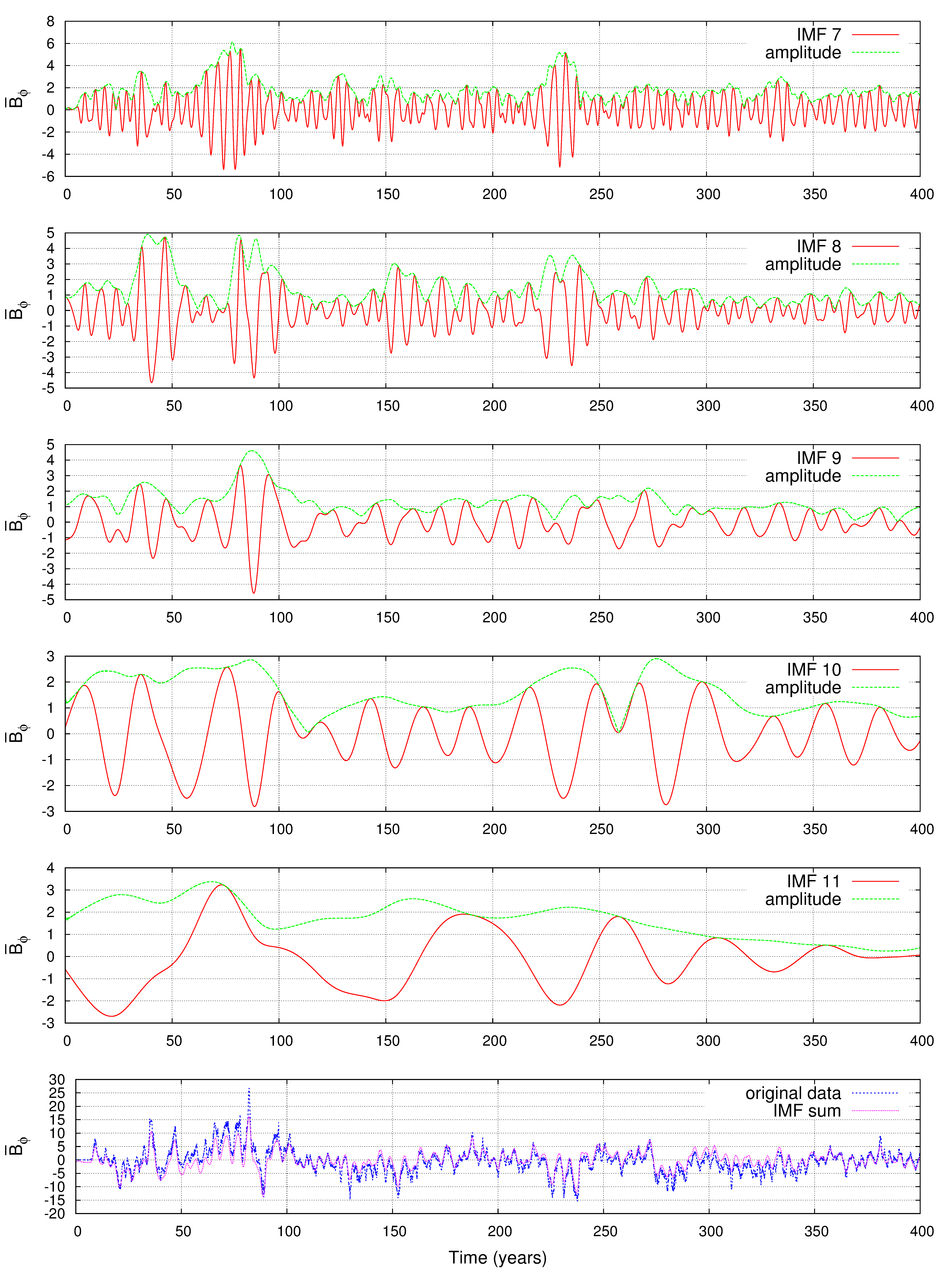
Figure 16: Modes 7–11 of $\overline{B}_{\phi}$ at $R_{\rm b}$ and latitude of $22^{\circ}$

.

Appendix B $D^{2}$ phase dispersion statistic

The $D^{2}$ phase dispersion statistic was first introduced in Pelt (1983). Recent applications of the method can be found in Lindborg et al. (2013), Karak et al. (2015), and Olspert et al. (2015). Similarly to EEMD, the $D^{2}$ statistic is well suited for non-stationary data. However, while EEMD aims at decomposing the initial time series into a set of quasi-harmonic signals, the purpose of $D^{2}$ is to find a set of average cycle lengths, $P_{\rm m}$, which are consistent with the full data set. The $D^{2}$ statistic is defined as follows:

$$D^{2}(P,\Delta t)=\frac{\sum\limits_{i=1}^{N-1}{\sum\limits_{j=i+1}^{N}{g(t_{i}}},t_{j},P,\Delta t)[f(t_{i})-f(t_{j})]^{2}}{2\sigma^{2}\sum\limits_{i=1}^{N-1}{\sum\limits_{j=i+1}^{N}{g(t_{i}}},t_{j},P,\Delta t)},$$ (14)

where $f(t_{i}),i=1,\dots,N$ is the input time series, $\sigma^{2}$ is its variance, $g(t_{i},t_{j},P,\Delta t)$ is the selection function, which is significantly greater than zero only when

$$t_{j}-t_{i} \approx kP,k=\pm 1,\pm 2,\ldots{\rm\ \ \ and}$$ (15)

$$\left|{t_{j}-t_{i}}\right| \lessapprox \Delta t,$$ (16)

where $P$ is the trial period and $\Delta t$ is the so-called coherence time, which is the measure of the width of the sliding time window wherein the data points are taken into account by the statistic. More precisely, in the given study the function $g$ has been chosen as the product of cosine and Gaussian functions. Here the former is depending only on the phase difference of given points w.r.t given trial period and the latter only on the time difference between the corresponding points:

$$g(t_{i},t_{j},P,\Delta t) = g_{1}(t_{i},t_{j},P)\cdot g_{2}(t_{i},t_{j},\Delta t),$$ (17)

$$g_{1}(t_{i},t_{j},P) = \frac{1}{2}\left(\cos\left(2\pi\cdot\rm{frac}\left(\frac{t_{j}-t_{i}}{P}\right)\right)+1\right),$$ (18)

$$g_{2}(t_{i},t_{j},\Delta t) = \exp\left(-\ln 2\left(\frac{t_{j}-t_{i}}{\Delta t}\right)^{2}\right).$$ (19)

As $\Delta t$ is made shorter, we match nearby cycles in a progressively narrower region, and consequently, estimate a certain mean cycle length $P_{\rm m}$, not necessarily coherent for the full time span. At large values of $\Delta t$, i.e. when the time window width approaches the time span of the data, the $D^{2}$ spectrum approaches the result that would be obtained using e.g. Fourier transform. More precisely, $P_{\rm m}$ is determined from the dispersion spectrum calculated for the longest coherence time for which the shape of the minimum is still symmetric and singular (with a single local minimum within reasonably narrow search region to exclude possible minima from higher harmonics). Denoting this optimal coherence time by $\Delta t_{\rm opt}$ we define the mean cycle length as:

$$P_{\rm m}=\underset{P}{\arg\min}\{D^{2}(P,\Delta t_{\rm opt})\}.$$ (20)

When visualizing the spectrum, we plot the cycle length $P$ on vertical axis, but instead of directly plotting the coherence time on horizontal axis, we use $\Delta t/P$ instead. This is just a count of cycles with a corresponding period that fit into the time interval equal to given coherence time. We call this entity coherence length.