Computer simulations of single particles in external electric fields

Abstract

Applying electric fields is an attractive way to control and manipulate single particles or molecules, e.g., in lab-on-a-chip devices. However, the response of nanosize objects in electrolyte solution to external fields is far from trivial. It is the result of a variety of dynamical processes taking place in the ion cloud surrounding charged particles and in the bulk electrolyte, and it is governed by an intricate interplay of electrostatic and hydrodynamic interactions. Already systems composed of one single particle in electrolyte solution exhibit a complex dynamical behaviour. In this review, we discuss recent coarse-grained simulations that have been performed to obtain a molecular-level understanding of the dynamic and dielectric response of single particles and single macromolecules to external electric fields. We address both the response of charged particles to constant fields (DC fields), which can be characterized by an electrophoretic mobility, and the dielectric response of both uncharged and charged particles to alternating fields (AC fields), which is described by a complex polarizability. Furthermore, we give a brief survey of simulation algorithms and highlight some recent developments.

I Introduction

Dispersions of nanoparticles in electrolyte fluids are ubiquitous in everyday life. Prominent examples are proteins and DNA in aqueous environment. The study of such systems is not only of technological interest for the development of advanced materials, but also of fundamental interest for our understanding of life science and biophysics. These materials have a large inherent complexity. Already the simplest system contains at least three components: large macromolecules or particles (solutes), small electrolyte ions, and solvent molecules. The interactions between the components include short-range interactions, such as excluded-volume and van der Waals interactions, and long-range interactions, such as the electrostatic and hydrodynamic interactions. The interplay of these interactions determines the equilibrium and dynamic properties of the system. Due to its multi-component nature, a wealth of parameters can be used to control material properties, e.g., the surface charge density, the salt concentration, the dielectric constant of the solvent. External perturbations can be used to manipulate the behaviour of the system. Since charges are involved, electric fields are particularly efficient.

In this review, we will focus on two important systems: Colloidal dispersions and polyelectrolyte solutions. Colloidal particles are solid objects with sizes ranging from a few nanometers to micrometers Russel et al. (1989); Dhont (1996). In electrolyte solution, an electric double layer forms near the solid/liquid interface and plays an important role in determining the dynamics. Polyelectrolytes are charged polymers, with DNA and protein being the most prominent examples Barrat and Joanny (1996); Dobrynin and Rubinstein (2005). In comparison to colloids, which have no internal degree of freedom, polyelectrolyte chains can change their conformation from a coil to a compact globule, and to extended rodlike structures. Counterions can bind to the polyelectrolyte backbone in the case of strongly charged chains, or form a diffusive layer. In both systems, it is important to consider the charged particle and its surrounding electric double layer as a whole.

Computer simulations have become a widely accepted approach to studying complex systems, complementing the well-established theoretical and experimental methods. For charged particles in electrolyte solutions, the main difficulty lies in the multi-scale nature of the system. Taking colloidal particles as an example, the length scales range from the size of the water molecules (around $10^{-10}$m), to the size of the colloidal particle in the order of $10^{-6}$m. Likewise, the dynamics of the system also involves processes with characteristic time scales spanning several orders of magnitude. For example, the characteristic diffusion time (the time to diffuse along one molecule/particle diameter) for small salt ions and large colloids is of the order of 10 picoseconds and seconds, respectively. In principle, one can use molecular dynamics simulation with atomistic detail Yeh and Hummer (2004), but even with current computer resources, the accessible time and length scales are still limited. One possible solution is to use coarse-grained simulations, which allow one to access larger length and time scales at the expense of losing fine scale details.

In this paper, we review recent coarse-grained simulation studies of charged colloids and polyelectrolyte chains in electrolyte solution. We mostly focus on the case of one single particle and its response to a weak and spatially homogeneous, albeit possibly time-dependent external electric field (linear response regime). We discuss the physical mechanism behind various dynamic processes driven by the external electric fields. Since there is a vast amount of theoretical and experimental literature on this subject, we shall not be comprehensive, but we will focus on presenting simulations that illustrate important physical mechanisms. We apologize in advance that our reference list is far from complete.

This review is organized as follows: We start with a brief discussion of simulation techniques in Section II. Then we turn to reviewing simulation studies of particles and polyelectrolyte chains under constant electric fields (DC fields) and alternating electric fields (AC fields) in Section III and IV, respectively. We conclude in Section V with a brief summary and perspective.

II Simulation Methods

When studying the dynamics of a system that includes large particles (colloids or polyelectrolytes) and small solvents/ions, one needs to consider both the electrostatic and hydrodynamic interactions. From a simulation point of view, modeling such a system is a challenging task, because both the electrostatic and hydrodynamic interactions are long-range. Taken separately, each interaction has been well studied in the literature Allen and Tildesley (1987); Frenkel and Smit (2002); Slater et al. (2009); Pagonabarraga et al. (2010); Smiatek and Schmid (2012); Cisneros et al. (2014). Methods can be grouped into the categories of “implicit” and “explicit” methods, Pagonabarraga et al. (2010); Smiatek and Schmid (2012), depending on whether the small components (solvents and ions) are simulated explicitly or replaced by effective interactions between large components. In this review, we shall focus on explicit methods. The inclusion of small ions and solvent particles requires more computational resources, but in many cases, this sacrifice is necessary for a proper treatment of the dynamics. For example, implicit methods that treat hydrodynamic interactions, e.g., at the level of an Oseen mobility matrix, are not capable of accounting for the effect of finite Reynolds numbers, and difficult to combine with complex boundary conditions. On the other hand, implicit methods that replace the effect of small ions by screened electrostatic potentials do not capture the multitude of complex dynamical processes involved in the electrophoretic or dielectrophoretic response of a particle to an electric field. In the following, we first mention some classical approaches which are commonly used in mesoscopic simulations, and then highlight a few new developments.

One popular method for treating Coulomb interactions is Ewald summation, which applies to point charges with periodic boundary condition Ewald (1921). The idea is to split the interaction into two contributions: one is short-ranged and has a cutoff, the other one is a smooth function which can be calculated efficiently in Fourier space. After optimization, Ewald summation scales as $O(\mathcal{N}^{3/2})$, where $\mathcal{N}$ is the total number of point charges. Several methods improve the scaling to $O(\mathcal{N}\ln\mathcal{N})$ by computing the Fourier part on a grid using fast Fourier transform. Notable examples are Particle-Particle-Particle Mesh (P3M) Hockney and Eastwood (1988); Deserno and Holm (1998a, b), Particle Mesh Ewald (PME) Darden et al. (1993), and Smooth Particle Mesh Ewald (SPME) Essmann et al. (1995). Methods that scale linearly $O(\mathcal{N})$ with the system size have also been proposed in the literature, such as the Fast Multipole Method Greengard and Rokhlin (1987), and methods based on the Maggs approach Maggs and Rossetto (2002); Rottler and Maggs (2004); Pasichnyk and Dünweg (2004). These methods require an expensive computational overhead or have a large prefactor in the linear scaling; thus Ewald-based methods are still the most common choice in mesoscopic simulations. Some of the methods mentioned here have been combined into a parallel library ScaFaCoS Arnold et al. (2013); Sca , which is freely available.

Mesoscale methods for simulating fluid dynamics are based on one simple observation: As long as one is mostly interested in hydrodynamic effects, the solvent dynamics can be replaced by an artificial dynamics as long as the relevant conservation laws (mass, charge, momentum, etc.) are satisfied. Therefore, one can design simple fluid models that can be simulated at low computational cost. Popular examples in the literature include the Lattice Boltzmann (LB) method, Dissipative Particle Dynamics (DPD), and Multi-Particle Collision Dynamics (MPCD). DPD is a particle-based method that uses soft potentials and pair-wise interactions Hoogerbrugge and Koelman (1992); Español and Warren (1995). LB is a lattice-based method which solves a linearized Boltzmann equation in a fully discretized fashion Succi (2001); Dünweg and Ladd (2009). In MPCD, the interactions between particles are performed by sorting particles in cells and followed by local operations Malevanets and Kapral (1999); Kapral (2008); Gompper et al. (2009). Besides these mesoscopic simulation methods, one can also solve the Navier-Stokes equations numerically, for example, in Fluid Particle Dynamics Tanaka and Araki (2000) and in the Smoothed Profile method Nakayama and Yamamoto (2005).

Once one settles on solvers for the electrostatic and hydrodynamic equations, the next step is to choose a simulation model for the large particle. In the case of polyelectrolytes, a common choice is the bead-spring model, which represents a polyelectrolyte as a chain of consecutive charged beads connected by springs. Large rigid particles, such as micrometer-sized colloids, can be introduced through appropriate boundary conditions, e.g., no-slip boundaries for the hydrodynamics and hard impenetrable boundaries for solvent and ion particles. An alternative approach suitable for smaller colloids is the so-called “raspberry model”, which represents the colloid by a shell made of of surface beads. The shape of the shell is maintained either by springs Lobaskin and Dünweg (2004) or by fixing the bead position with respect to the colloid center Chatterji and Horbach (2005).

The computational expenses for the electrostatic and hydrodynamic computations are not equivalent. At high salt concentrations, a comparison Smiatek et al. (2009) has shown that the computational time is dominated by the costs of treating the charges. Unfortunately, as mentioned above, implicit models for small ions are not suitable for dynamic studies. We recently proposed an efficient algorithm that overcomes the bottleneck caused by the explicit charges Medina et al. (2015). It makes a compromise between computing efficiency and taking full consideration of correlations at all scales. The evolution of the ionic concentration is computed using Brownian pseudo particles Szymczak and Ladd (2003), which is very fast because pseudo particles have no direct pair interactions. In this approach, one chooses a coarse-grained length scale. Short-range correlations between small ions on length scales shorter than the coarse-grained length are neglected, but long-range charge-charge correlations can be retained. The full method consists of the pseudo-ion solver for electrolytes, DPD for the fluid and a P3M Coulomb solver. Simulations of electro-osmosis showed that the computer time required for the electrostatic calculations can be reduced to about half the time required for treating the fluid. Moreover, since the number of pseudo particles can be chosen independently of the number of ions, it is independent of the ion concentration. Therefore, the proposed method is particularly suited for electrolyte solutions at high salt concentrations.

Another issue in electrostatic simulations is the dielectric constant, which is often assumed to be homogeneous throughout the simulation box. In reality, the dielectric permittivity in the water and in the nanoparticles differ significantly. The difficulty to include dielectric contrast in molecular dynamics lies in the calculation of induced polarization charge at the interfaces, which has to be done self-consistently in every time-step. Recently, a number of authors have addressed this problem Tyagi et al. (2010); Jadhao et al. (2012); Barros et al. (2014). For example, Barros et al. Barros et al. (2014) proposed to use a Generalized Minimum Residual method Saad and Schultz (1986) to calculate the distribution of surface bound charges on nanoparticles and applied this approach to study the self-assembly of binary colloids. They observed an unexpected string structure formation due to the dielectric effect Barros and Luijten (2014). Boundary methods such as that sketched above also open up the possibility to study phenomena associated with induced-charge electrokinetics Bazant and Squires (2004). However, they cannot be used to simulate media with a smoothly varying dielectric constant $\epsilon(\mathbf{r})$. Such systems can be treated using the recently proposed Maxwell Equations Molecular Dynamics (MEMD) method Rottler and Maggs (2004); Pasichnyk and Dünweg (2004), which is based on the Maggs approach Maggs and Rossetto (2002) and solves the Maxwell equations by propagating a set of virtual auxiliary fields on a local scale. A recent review on methods to deal with dielectric contrasts can be found in Ref. Arnold et al. (2013).

III Particles in Constant Electric Fields

Let us now consider an object (molecule or colloid) with a characteristic size of $a$ suspended in an electrolyte solution. The object can acquire surface charges by several means, either by the dissociation of protons or by the selective adsorption of ions from the aqueous solution. Due to the electrostatic interaction, it is surrounded by a so-called “electric double layer” of oppositely charged ions. Some of these may bind strongly to the surface (Stern layer), and their main effect is to reduce the effective surface charge. The others form the “diffuse layer”, which is characterized by a constant turnover of weakly bound, mobile ions. The thickness of the diffuse layer results from the competition of osmotic pressure and electrostatic interactions and is typically of the order of the Debye screening length $\kappa^{-1}$. Both $\kappa^{-1}$ and the particle extension, $a$, represent important characteristic lengths of the system. When an external electric field $\mathbf{E}$ is applied, a positively charged particle starts to move in the direction of the electric field, and the ions in the diffuse layer experience a force in the opposite direction. Thus the particle experiences a friction force exerted by the electrolyte fluid which prevents its movement. In the stationary case, the electric driving force and the friction force balance each other and the object moves with a constant velocity $\mathbf{v}$. The ratio between the terminal velocity $\mathbf{v}$ and the applied electric field $\mathbf{E}$ is called electrophoretic mobility $\mu$,

$$\mathbf{v}=\mu\mathbf{E}.$$ (1)

In general, the electrophoretic mobility is a tensor, but we shall here restrict the discussion to isotropic objects, in which case the mobility is a scalar quantity.

Before we proceed to presenting simulations, we briefly recapitulate the main contributions to the friction force involved in electrophoresis Lyklema et al. (1995)

1. The viscous force $\mathbf{F}_{\mathrm{vis}}$ exerted by the fluid. The magnitude of this force is given by the Stokes friction $F_{\mathrm{vis}}=-6\pi\eta av$, where $\eta$ is the shear viscosity of the fluid.

2. The electrophoretic retardation force $\mathbf{F}_{\mathrm{ret}}$ due to the movement of the counterion cloud. Since the counterions have the opposite charge, they move in the opposite direction of the central object. Ideally, the counterions compensate the charged object and the whole system is charge neutral. Therefore, the electrostatic force on the counterions exactly cancels the driving force on the object, but to which extent this force is transferred to the central object is complicated.

3. The polarization force $\mathbf{F}_{\mathrm{pol}}$ due to the distortion of the counterion cloud. As an example, let us consider a spherical colloid. The charge centers of the colloid and its surrounding counterions coincide at zero external field. If an external field is applied, the two centers are displaced slightly as the counterion cloud is distorted, which induces a dipole moment. The central object experiences an extra electric force due to this distortion.

III.1 Electrophoresis of Colloidal Particles

In general, the electrophoretic mobility of colloids depends on several parameters, e.g., the colloidal size $a$, the Debye screening length $\kappa^{-1}$, and the surface potential at the plane of shear, termed the $\zeta$-potential. In simulation studies, it is sometimes easier to prescribe the surface charge density $\sigma$. Unfortunately, the relation between $\sigma$ and $\zeta$ is not simple Doane et al. (2011); analytic formulas only exist for simple geometries (planes and cylinders). The electrophoretic mobility has a simple form only for special cases such as weakly charged colloids ($\zeta/k_{B}T\ll 1$). In this limit, the counterion distribution can be treated using the Debye-Hückel approximation. Two well-known results are the Hückel and Smoluchowski formulae: If the electric double layer is thick ($\kappa a\ll 1$), one can neglect the retardation and polarization forces, and write the electrophoretic mobility as Hückel (1924)

$$\mu=\frac{2}{3}\frac{\varepsilon}{\eta}\zeta\quad(\kappa a\ll 1),$$ (2)

where $\varepsilon$ is the permittivity of the solution. This formula is derived from the balance between the electric driving force and Stokes friction.

In the opposite limit of thin electric double layers, one obtains the Smoluchowski formula Smoluchowski (1917)

$$\mu=\frac{\varepsilon}{\eta}\zeta\quad(\kappa a\gg 1).$$ (3)

In this case, the retardation force is accounted for but the polarization force is neglected. The situation is different if the surface charge is kept constant. In this case, the surface potential vanishes for large $\kappa a$, resulting a zero mobility.

For intermediate values of $\kappa a$, Henry derived an analytic formula of the form Henry (1931)

$$\mu=f(\kappa a)\frac{\varepsilon}{\eta}\zeta$$ (4)

with a scaling function $f(\kappa a)$ that interpolates between the Hückel and Smoluchowski result in their corresponding limits: $f(\kappa a)\to 1$ for $\kappa a\ll 1$ and $f(\kappa a)\to 2/3$ for $\kappa a\gg 1$.

The assumptions and approximations made in deriving these simple formulae are:

• The distortion of the counterion cloud is assumed to be negligible, and the contribution from the polarization force $\mathbf{F}_{\mathrm{pol}}$ is omitted.

• The distribution of salt ions and counterions is treated at the mean-field level using a continuum approximation. In equilibrium, this corresponds to the Poisson-Boltzmann approximation. Short-range correlations between charged species are neglected.

• The colloidal particle is assumed to be weakly charged ($e\zeta/k_{B}T<1$). This assumption justifies the use of the Debye-Hückel approximation, and the simplification of the Poisson-Boltzmann equation to a linear equation facilitates the derivation of analytic expressions. In this limit, the counterion distribution near the charged surface decays exponentially with the characteristic length $\kappa^{-1}$.

We shall now discuss how theoretical considerations and numerical calculations in the last few decades have helped to probe phenomena which are beyond those approximations.

III.1.1 Methods Based on the Electrokinetic Equations

A general framework to study the dynamic phenomenon in electrolyte solutions is provided by the electrokinetic equations Russel et al. (1989). This involves a change in the point of view: Instead of calculating the friction force on the charged colloids, one writes down explicitly a set of partial differential equations which governs the dynamics of electrolyte solutions at the level of a continuum theory. The electrokinetic equations have three basic constituents: The Poisson equation for the electrostatic potential, the Navier-Stokes equations characterizing the fluid flow, and the Nernst-Planck equation, which is basically a convection-diffusion equation describing the time evolution of ionic concentration profiles. Since thermal fluctuations and the discrete character of charges are neglected in this continuum approach, it corresponds to a mean-field approximation and reproduces the Poisson-Boltzmann results at equilibrium. All components of the friction force are implicitly included in this approach.

In an early seminal paper O’Brien and White (1978), O’Brien and White computed the electrophoretic mobility of a single sphere in an infinite domain by numerically solving the electrokinetic equations for weak external fields (linear regime). Their results differed qualitatively from the previous predictions in the case of the thin electric double layer: Instead of being a monotonically increasing function of the zeta-potential $\zeta$, as predicted by Eq. (3) , the mobility has a maximum for values of $\kappa a>3$. This is shown in Fig. 1, right. The non-monotonic behaviour results from the fact that different competing factors contributing to electrophoresis scale differently with $\zeta$: The electrostatic driving force is proportional to $\zeta$, while the friction force associated with the distorted counterion cloud is proportional to $\zeta^{2}$.

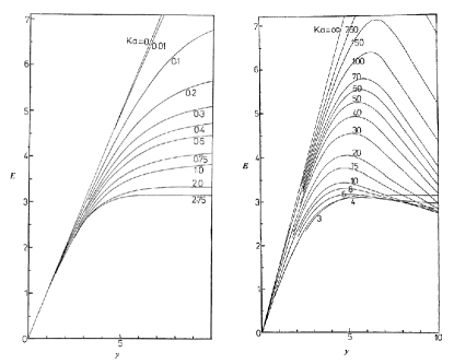
Figure 1: Reduced mobility $E=(6\pi\eta e/\varepsilon k_{B}T)\mu$ as a function of the reduced zeta potential $y=(e/k_{B}T)\zeta$. Left: The mobility is a monotonic function for thick electric double layers $\kappa a<3$. Right: A mobility maximum appears for thin electric double layers, $\kappa a>3$. Reprinted from Ref. O’Brien and White (1978) with permission from The Royal Society of Chemistry.

Based on the same electrokinetic model, Schmitz and Dünweg Schmitz and Dünweg (2012) recently developed a lattice-based approach to solve the linearized electrokinetic equations. Their strategy is divide-and-conquer: They divided the original equations into parts, and developed different numerical solvers for each equation. They then combined different solvers to compute the original equations using an iteration procedure. Their method is different to O’Brien and White in two aspects: One is the usage of periodic boundary condition, which allows to study the effect of colloid concentration. The second difference is that no assumption is made about the colloid shape, and one can in principle study colloidal particle with irregular shape.

It is also possible to start with the full electrokinetic equations instead of the linearized version. The three equations belong to different categories of partial differential equations, and there exist efficient solvers for each equation separately. Based on the Lattice Boltzmann method, Giupponi and Pagonabarraga studied the electrophoretic mobility of charged colloids Giupponi and Pagonabarraga (2011). The Nernst-Planck equation was solved using a discrete method Capuani et al. (2004). The results match those of O’Brien and White well in the case of small zeta-potentials, but deviate when the zeta-potential is large. In this regime, the method used by O’Brien and White suffers from numerical problems O’Brien and White (1978), which may explain the discrepancy. In particular, Giupponi and Pagonabarraga found that a mobility maximum exists for all salt concentrations. They further investigated the effect of diffusivity of the small ions.

Kim et al. took a different approach to the fluid by solving the Navier-Stokes equations directly Kim et al. (2006). The difficulty lies in the proper and efficient treatment of the moving boundary of the colloids. They devised the Smoothed Profile method, which replaces the shape boundary by a smooth interface with finite thickness Nakayama and Yamamoto (2005). Their results for the electrophoretic mobility showed good agreement with O’Brien and White for thick electric double layer ($\kappa a=0.5$). The efficiency of their numerical method permits the simulation of many colloids in one simulation box. They further investigated the mobility dependence on the colloid concentration and compared their results with the theoretical prediction of Ohshima Ohshima (1997). At low colloid concentration, the agreement between the simulation and theory is good. Deviations become noticeable when the electric double layers from different colloids overlap.

III.1.2 Particle-based Simulations

All studies based on the electrokinetic equations neglect short-range correlations, as the small ions are treated in terms of ionic concentration fields. To remove this approximation, one must simulate the small ions as particles with excluded volume interactions that carry discrete charges. Combined with mesoscopic methods for the fluid, one obtains a simulation scheme which accounts for correlations between charged species. One drawback is an increase in computational time which makes the simulation of large colloids very difficult.

Lobaskin et al. studied the electrophoresis of charged colloids in electrolytes containing only counterions or with very low salt content Lobaskin et al. (2007); Dünweg et al. (2008). In their approach, the fluid is simulated using the LB method, and the colloidal particle is modeled using the raspberry model Lobaskin and Dünweg (2004). Using a dimensional analysis, they demonstrated that the reduced electrophoretic mobility, defined by $\mu_{\rm red}=\mu/\mu_{\rm H}$ ($\mu_{\rm H}$ is the Hückel result, Eq. 2), depends only on two dimensionless parameters $Z_{\rm eff}l_{B}/a$ and $\kappa a$. Here $Z_{\rm eff}$ is the effective charge of the colloid, which differs from the bare colloid charge $Z$ by the amount of strongly adsorbed counterions, $l_{B}=e^{2}/4\pi\varepsilon k_{B}T$ is the Bjerrum length, and the inverse screening length $\kappa$ is defined as

$$\kappa^{2}=4\pi l_{B}(c_{i}+c_{s}),$$ (5)

where $c_{i}=Z/V$ is the counterion concentration and $c_{s}$ is the ionic concentration due to the salt ions. Based on the dimensional analysis and Eq. (5), one can map the mobility of colloids in salt-free fluids (the number of counterions is set by the colloid concentration) to that in electrolytes containing a small amount of salt at the same value of $\kappa a$. This correspondence is confirmed by both the simulations and experiments Lobaskin et al. (2007).

A similar model was used by Chatterji and Horbach in a series of studies of highly charged colloids Chatterji and Horbach (2005, 2007, 2010). They varied the colloid charge density instead of the zeta potential because the former can be controlled more easily in simulations. Upon increasing the charge density, the electrophoretic mobility was found to initially increase, then reach a maximum, and decrease again. These simulation results are in accordance with the predictions for the thin electric double layer case (Fig. 1, right).

Chatterji and Horbach also considered systems containing divalent counterions, in which they found the electrolyte mobility to be reversed at high charge density, indicating an overcompensation of the surface charge by the multivalent counterions. This overcharging phenomenon can be explained by ion correlations Quesada-Pérez et al. (2003) and has also been observed experimentally. In experiments, however, the effect is sometimes larger than predicted by numerical simulations, suggesting that it might be enforced by ion specific attractive forces Semenov et al. (2013). Recent simulations by Raafatnia et al. have shown that overcharging may even occur in electrolytes containing only monovalent ions if the colloids are coated by a suitable organic layer Raafatnia et al. (2014a); Raafatnia et al. (2015).

As mentioned above, treating colloids with sizes much larger than the ion size is difficult with explicit ion models. Raafatnia et al. have developed a hybrid approach to studying the electrophoresis of large colloids Raafatnia et al. (2014b). They first measured the zeta-potential of a flat surface using simulations with explicit microions. The measured zeta-potential was then used as an input in the electrokinetic equations to calculate the electrophoretic mobility. When compared with experiments, the scheme worked well for monovalent and divalent salt solutions. In the case of trivalent salt, they needed to introduce an attractive interaction in order to reproduce the mobility reversal which is observed experimentally.

III.2 Polyelectrolytes

We turn to discussing polyelectrolyte electrophoresis. Compared to colloid electrophoresis, there are several differences:

• Colloidal particles are usually at least one order of magnitude larger than the small molecules (solvents and salt ions). The separation of length scales makes it possible to describe large colloids in terms of boundary conditions and motivates the use of continuum approaches. In the case of polyelectrolytes, the size of the monomer units is comparable to that of small molecules and the application of boundary methods becomes questionable. Even though the zeta potential is sometimes used to parameterize experimental results, its physical meaning is not always obvious. In simulations, an explicit treatment of small ions is often more appropriate than the use of continuum theories.

• Whereas colloidal particles are rigid objects, polyelectrolyte chains can assume many conformations. The conformational dynamics is strongly influenced by the electrostatic and hydrodynamic interactions between monomers. Therefore, a full treatment of both interactions is necessary. Implicit methods have been designed to circumvent this requirement for stationary situations Hickey et al. (2010, 2012), but in general, one has to be careful when dealing with non-stationary states. The conformational flexibility complicates studies of electrophoretic mobility.

• If polyelectrolytes are highly charged, the strong electrostatic interaction attracts counterions to the proximity of the chain backbone. This phenomenon, called Manning condensation Manning (1969), also influences the electrophoretic mobility.

• In the case of colloidal particles, the size and the surface charge density can be adjusted independently. For polyelectrolytes, this is usually not the case. The control parameters are the chain length $N$ and the charge fraction. We shall restrict ourselves to strongly charged chain, where each monomer carries a unit charge. The size of a polyelectrolyte chain is characterized by the radius of gyration $R_{g}$, which depends on the chain length. Therefore, the electrophoretic mobility is usually represented as a function of the chain length.

III.2.1 Free Solution Electrophoresis

When the size of polyelectrolyte chain is much smaller than the Debye screening length, $\kappa R_{g}\ll 1$, one may invoke the Hückel picture for colloidal particles and consider only the electric driving force and the viscous friction. The driving force of the external field is proportional to the chain length, while the viscous force from the fluid also increases with the chain length, but to a smaller extent due to the hydrodynamic interactions. Monomers experience hydrodynamic drag and shield each other from the exposure to the outer fluid, which effectively reduces the total Stokes friction. Therefore, for short chains, the mobility increases with the chain length.

This behaviour was indeed observed in simulations and experiments. Grass and Holm modeled the polyelectrolyte as a chain of charged beads connected by finitely extensible nonlinear elastic bonds Grass et al. (2008). The fluid was simulated using the LB method, and the Coulomb interaction was calculated using the P3M method. They computed the electrophoretic mobility from equilibrium simulations using the corresponding Green-Kubo relation. Later they also directly measured the terminal velocity in an external electric field Grass and Holm (2009, 2010), and found that the results agree in the weak-field regime. Frank and Winkler used a similar model for the polyelectrolyte chain, but simulated the fluid using MPCD Frank and Winkler (2008). Both studies emphasize the importance of hydrodynamic interaction, as complementary Langevin simulations show a decrease in the mobility with increasing chain length.

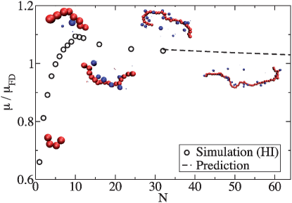
Figure 2: Reduced electrophoretic mobility $\mu$ of a polyelectrolyte chain as a function of the chain length $N$. The mobility is scaled with the free-draining limit $\mu_{\rm FD}$. Reprinted from Ref. Grass and Holm (2009) with permission from The Royal Society of Chemistry.

One peculiar observation in these simulations is the presence of a mobility maximum at chain lengths $N\sim 10$ (see Fig. 2). This was attributed to a reduction of the effective charge of the polyelectrolyte chain, which reduces the electric driving force. As the chain becomes longer, the polyelectrolyte assumes a rod-like conformation due to the mutual repulsion of monomers, and Manning condensation sets in. The accumulation of counterions on the backbone reduces the effective charge of the chain, thereby reducing the electric driving force. Frank and Winkler measured the number of condensed counterions in their simulation using a distance criterion Frank and Winkler (2008). They found that as the chain becomes longer, the ratio between the condensed counterion to the total charge of polyelectrolyte chain approaches $1-1/\xi$, where $\xi$ is the Manning parameter. Grass and Holm applied different estimators for the effective charge, with similar results Grass and Holm (2009). However, the exact point at which the saturation is reached is still unclear, because the polyelectrolyte chain is flexible, whereas the theory of Manning condensation applies for rigid rods.

When the chain length increases further, the electrophoretic mobility reaches a constant value. This so-called “free-draining” limit has been well studied in the literature Manning (1981); Barrat and Joanny (1996). The fact that the mobility does not depend on the length of the polymers prevents the separation of long polyelectrolyte chains by free solution electrophoresis. The physics behind the plateau in mobility is two-fold: On the one hand, the effective charge per monomer becomes a constant, once the Manning condensation sets in. Therefore, the electric driving force is proportional to the chain length. On the other hand, the effective friction force opposing the electric force also scales linearly with the chain length once the polyelectrolyte size becomes larger than the Debye screening length. This is because a long chain can be viewed as a chain of charge neutral blobs with the blob size being the Debye length. When applying an external electric field, the chain experiences a force, but the surrounding counterions experience a force in the opposite direction, such that the sum of all forces on charged particles in a blob is zero. Therefore, no flow is induced, the hydrodynamic interactions associated with the electric force are screened Kekre et al. (2010), and the resulting electrophoretic mobility does not depend on the chain length.

III.2.2 Effect of Adding Salt

The hydrodynamic screening effect discussed above becomes even more pronounced in the presence of salt. Salt plays a dual role in polyelectrolyte electrophoresis, because it screens both the electrostatic and the hydrodynamic interactions. The screened electrostatic potential decays exponentially with a characteristic length $\kappa^{-1}$. The screened hydrodynamic flow profile still features a long-range $1/r^{3}$ decay, which is due to the vectorial nature of the velocity field Long and Ajdari (2001). In free solution, the screening length for hydrodynamics $\kappa_{\mathrm{H}}^{-1}$ coincides with the Debye screening length $\kappa^{-1}$. Therefore, varying the salt concentration induces a complicated interplay between the electrostatic and hydrodynamic interactions. In Ref. Grass and Holm (2010), Grass and Holm examined the effect of salt on the electrophoretic mobility of short polyelectrolyte chains. The increase in the salt concentration reduces the screening length $\kappa_{\mathrm{H}}^{-1}$ and therefore reduces the initial shielding of hydrodynamics. As a result, the electrophoretic mobility becomes almost length-independent at high salt concentration. Fischer et al. Fischer et al. (2008) found that the counterion mobility changes sign as a function of salt concentration. At low salt concentration, the counterions condense to the polyelectrolyte backbone and the hydrodynamic drag forces the counterions to move together with the polyelectrolyte chain. At high salt concentrations, however, the screening of hydrodynamics decouples the motion of counterions and polyelectrolyte, and counterions move in the opposite direction of the polyelectrolyte.

III.2.3 Effect of Confinement

Another way of decoupling the screening lengths for electrostatics and hydrodynamics is to use confinement. The screening length for hydrodynamics is given by either the characteristic size of the confinement or the Debye length, depending on which is smaller. Hickey et al. investigated the electrophoretic stretching of a polyelectrolyte chain confined between parallel plates Hickey et al. (2014). They found that the hydrodynamic interaction is screened by the confining walls for strongly confined chains. Their study focused on uncharged walls. In the case of charged wall, the electroosmotic flow induced by the counterions from the charged surface can reverse the movement of the polyelectrolyte chain: a positively charged polyelectrolyte chain can move in the opposite direction of the external field if confined by negatively charged walls Smiatek and Schmid (2010, 2011).

IV Particles in Alternating Electric Fields

Alternating electric fields (AC fields) provide another attractive tool for manipulating particles. Compared to constant electric fields (DC fields), one has several advantages:

• In homogeneous AC fields, the displacement of the charged particle averages to zero. This is in contrast to the DC case, where particles may travel over long distances during the time of an experiment. Since charged particles are mostly stationary, electrodes can be placed close to each other. Therefore, one can produce large value of the electric field, which is in general difficult in the DC case.

• Using AC fields, one can avoid the accumulation of charged species on electrodes.

• Unlike DC fields, AC fields do not generate constant electro-osmotic flows.

• Apart from the amplitude, one can also tune the frequency and the phase of AC fields. Since dynamical processes in the system can take place on different time scales, a time-dependent perturbation can probe the dynamics on selective time scales.

• Finally, AC fields can also be used to manipulate uncharged particles. This is because they can induce polarization charges both in charged and uncharged particles, and the polarized particles can then be further manipulated by applying electric field gradients.

IV.1 Colloidal Particles

The dielectric response to AC fields can be characterized by the polarizability $\alpha(\omega)$, where $\omega$ is the field frequency. In analogy to the electrophoretic mobility, the polarizability is defined as the ratio between the induced dipole moment and the external field,

$$\mathbf{p}=\alpha(\omega)\mathbf{E}.$$ (6)

The dipole moment has contributions from the colloidal particle and its surrounding electric double layer. In general, the polarizability depends on both the frequency and the amplitude of the external field. In weak fields, however, linear response applies and the polarizability does not depend on the field strength. In strong electric fields, nonlinear effects may become important.

One important application of AC fields is dielectrophoresis Pohl (1978); Jones (1995). In dielectrophoresis, the time-averaged force on a particle has the form $\Re\{\alpha(\omega)\}\nabla|\mathbf{E}|^{2}$, where $\Re\{\alpha(\omega)\}$ is the real part of the complex polarizability. Under the influence of a position-dependent AC field, the particle is driven along the direction of the field gradient Salonen et al. (2005, 2007); Zhao (2011). The magnitude of the force depends on the polarizability of the particle, which permits separation of colloidal particles and biomacromolecules Regtmeier et al. (2007). In a spatially homogeneous setup, AC fields can be used to control the self-assembly of many particles Grzelczak et al. (2010). The control is realized by tuning the induced dipole-dipole interaction between particles. The most important quantity in this context is the complex polarizability of the charged particle. Here we shall focus on studies of single colloidal particle and its polarizability under a homogeneous field.

IV.1.1 Maxwell-Wagner Theory and Electrokinetic Theory

The calculation of the induced dipole moment of a single spherical particle immersed in the medium provided by an electrolyte solution is a classical problem in electrodynamics, known as Maxwell-Wagner mechanism of dielectric dispersion Maxwell (1954); Wagner (1914). The complex polarizability $\alpha(\omega)$ has the form

$$\alpha(\omega)=4\pi\varepsilon_{\rm m}a^{3}\mathcal{K}(\omega)=4\pi\varepsilon_{\rm m}a^{3}\frac{\varepsilon_{\rm p}^{*}-\varepsilon_{\rm m}^{*}}{\varepsilon_{\rm p}^{*}+2\varepsilon_{\rm m}^{*}},$$ (7)

where $\mathcal{K}(\omega)$ is the Clausius-Mossotti factor. The system is characterized by the complex dielectric functions $\varepsilon_{\rm p,m}^{*}=\varepsilon_{\rm p,m}+K_{\rm p,m}/i\omega$, where $\varepsilon$ is the permittivity and $K$ the conductivity, and the subscript (${\rm p,m}$) labels the particle or the medium. From the form of the complex dielectric constant, one notices that the permittivity contribution dominates at high frequency ($\omega\rightarrow\infty$), while the conducting properties are more important at low frequency ($\omega\rightarrow 0$). The frequency separating these two limits is the inverse of the Maxwell-Wagner relaxation time

$$\tau_{\mathrm{mw}}=\frac{\varepsilon_{\rm p}+2\varepsilon_{\rm m}}{K_{\rm p}+2K_{\rm m}}.$$ (8)

For charged colloids, the electric double layer introduces another contribution to the dipole moment. O’Konski proposed a surface conductance term to account for the effect of electric double layer O’Konski (1960), and the same mechanism was also extended to the study of ellipsoidal colloids Saville et al. (2000). The Maxwell-Wagner-O’Konski theory has a simple analytic formulation which gives qualitatively correct predictions, but it suffers from one main drawback: Since the theory is entirely formulated in terms of macroscopic properties, such as the conductivities and permittivities, the polarization charges are taken to be localized at the particle/medium interface, and their spatial distribution is entirely neglected. This simplification is only justified for thin electric double layers and in the high-frequency regime.

Experiments revealed another dispersion in the low-frequency regime, which cannot be explained by the Maxwell-Wagner-O’Konski theory. This low-frequency dispersion, often called alpha-relaxation, results from the distortion of the electric double layer. To properly treat the electric double layer, one can resort to the electrokinetic equations. Dukhin and Shilov made the further assumption that the electric double layer is at local equilibrium with the surrounding bulk solution Dukhin and Shilov (1974), which is only valid in the low-frequency regime. They derived an analytic theory for the thin electric double layer case, which correctly predicts the low-frequency dispersion. The theory has been extended to asymmetric electrolytes Hinch et al. (1984); Chassagne et al. (2003); Grosse (2009a, b) and to aspherical colloids Chassagne and Bedeaux (2008).

In situations that involve thick electric double layer and the whole frequency spectrum, one can solve the full electrokinetic equations using a variety of numerical methods. DeLacey and White DeLacey and White (1981) extended the method of O’Brien and White O’Brien and White (1978) to AC fields and presented numerical solutions for the polarizability of a single spherical colloid DeLacey and White (1981). The electrokinetic equations are linearized in term of the external field, thus the calculation assumes weak fields. The method was further refined by Mangelsdorf et al. Mangelsdorf and White (1992, 1997) and Zhou et al. Zhou et al. (2005). Hill et al. developed an alternative numerical scheme which overcomes a numerical instability in the high-frequency regime Hill et al. (2003a), and extended the method to polymer-grafted particles Hill et al. (2003b); Hill and Saville (2005). The effect of the colloid concentration can also be incorporated by performing the calculations in a sphere, whose volume is equal to the inverse of the colloid number density Carrique et al. (2008a, b); Roa et al. (2012). Shih et al. applied the Smoothed Profile method Kim et al. (2006) to study the response of charged colloids to AC fields and reproduced both the Maxwell-Wagner relaxation and the alpha-relaxation Shih and Yamamoto (2014); Shih et al. (2015).

The numerical methods were also extended to rodlike particles. Zhao investigated the case of long parallel rod with two spherical caps on both ends Zhao and Bau (2010). The calculation showed that the transition frequency in the low-frequency dispersion is reduced when the rod becomes longer, and do not change once the rod length reaches a certain limit. Dhont and Kang developed theories based on electrokinetic equations to study two special cases: Very weakly charged rods where the dipole moment is mainly induced by the obstacle of the solid colloids Dhont and Kang (2010), and strongly charged rods where condensed counterions fully compensate the bare rod charge Dhont and Kang (2011).

IV.1.2 Simulations with Explicit Ions

The present authors have used particle-based method to investigate the dielectric response of a charged nanometer-sized colloid Zhou and Schmid (2012, 2013a); Zhou et al. (2013); Zhou and Schmid (2013b). The fluid dynamics is simulated using DPD, where small ions are included explicitly as charged beads with excluded-volume interactions. The large colloid is modeled using the raspberry model. We systematically investigated the complex polarizability $\alpha\{\omega\}$ as a function of the frequency, shown in Fig. 3.

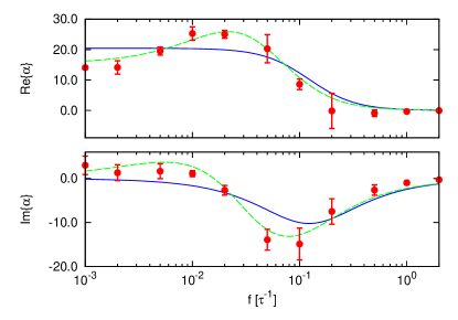
Figure 3: Real and imaginary part of the complex polarizability $\alpha(\omega)$ of a charged particle as a function of the frequency. The field strength is set in the linear region. The points with err-bars are simulation results. The solid lines give the prediction from the Maxwell-Wagner-O’Konski theory. The dashed lines are numerical solutions to the electrokinetic equations Hill and Saville (2005). Reprinted from Ref. Zhou and Schmid (2013b).

Let us first discuss the situation in the low-frequency regime. In the absence of an external field, the system including the charged colloid and its surrounding electric double layer has spherical symmetry. When an external field is applied, the colloid (positively charged) moves in the direction of the electric field, while the counterions move in the opposite direction. This creates a dipole moment, which points in the same direction than the external field. It also distorts the electric double layer, compressing it at the front end and expanding it at the back end, and thus creates a concentration gradient from back to front. In addition, the colloid acts as a moving obstacle for the salt ions in solution which are also driven by the electric field. Negatively charged ions accumulate at the front end of the colloid, which combined with the extra counterions results in a further increase of the salt concentration there, whereas the concentration at the back is further reduced. The concentration gradient induces a diffusive migration of the salt molecules from the front to the back. This concentration-induced effect reduces the dipole moment created by the external field. However, since it is a second-order effect caused by the field-induced dipole, the net dipole moment still points in the direction of the external field. This can be seen from Fig. 3, where the real part ${\rm Re}\{\alpha\}$ has a positive value at low frequency.

The diffusion of the salt over the distance of colloid diameter requires time, which can be estimated by

$$\tau_{\rm c}\sim\frac{(2a)^{2}}{D_{i}},$$ (9)

where $D_{i}$ is the diffusion constant of the small ions. If the field frequency increases beyond $1/\tau_{\rm c}$, the external field oscillates so fast that the diffusion process cannot follow. Therefore, the concentration-induced process is suppressed at frequencies $f>1/\tau_{\rm c}$, which effectively increases the dipole moment. This is the origin of the low-frequency dispersion and explains the slight increase of $\Re\{\alpha\}$ in Fig. 3.

When the frequency is further increased, the external field eventually oscillates so fast that the ion cloud cannot respond. Thus, both ${\rm Re}\{\alpha\}$ and ${\rm Im}\{\alpha\}$ drop to zero. The characteristic time corresponds to the time required for the small ions to diffuse over the distance of Debye length

$$\tau_{\rm mw}\sim\frac{\kappa^{-2}}{D_{i}}=\frac{\varepsilon_{\rm m}}{K_{\rm m}}.$$ (10)

The last equality applies for our simulation parameters ($\varepsilon_{\rm m}=\varepsilon_{\rm p}$ and $K_{\rm p}=0$), which differs from Eq. (8) only by a prefactor.

The simulation results can be compared with the theoretical and numerical predictions. The Maxwell-Wagner-O’Konski theory gives the solid curves in Fig. 3, which are only in qualitative agreement with the simulation. The theory predicts roughly the correct transition frequency in the high-frequency regime, but misses the low-frequency dispersion. The numerical solution of the electrokinetic equations is shown with dashed lines. It is in quantitative agreement with the simulation results.

We have also investigated the dielectric response of uncharged colloids to external AC fields Zhou and Schmid (2013a). The Maxwell-Wagner theory, Eq. (7), predicts a complex polarizability, simply due to the fact that the medium is conducting and the particle is not. Physically, the particle acts as an obstacle for the flow of charges induced by the applied field, such that charges of opposite sign accumulate at both ends. Since uncharged particles have no electric double layer, one does not expect additional contributions. Indeed, the simulation data were found to be in almost perfect agreement with the predictions of the Maxwell-Wagner theory. Fine details of the charge distributions can be understood quantitatively within the electrokinetic theory developed by Dhont and Kang Dhont and Kang (2010).

IV.2 Polyelectrolytes

Simulating the polyelectrolyte response to AC fields is a challenging task and only a few researchers have tackled this problem. Most studies focused on the conformational change of a single polyelectrolyte chain when a strong field is applied. For polyelectrolyte chains that are sufficiently long, or in the case of high salt concentration, hydrodynamic interactions are strongly screened. Therefore, most simulation studies used a Langevin thermostat which neglects the hydrodynamics, but includes small ions explicitly in order to account for the Manning condensation.

Liu et al. studied the unfolding and collapse of a flexible polyelectrolyte under a sinusoidal electric field Liu et al. (2010). They first measured the critical field strength at which the chain undergoes a transition to the fully extended state. Their results confirmed a theoretical prediction by Netz Netz (2003a, b): The critical field scales as $E_{\rm crit}\sim N^{x}$, where $x=-1/2$ for collapsed chains and $x={-3\nu/2}$ for non-collapsed chains with the Flory exponent $\nu$. They also estimated the relaxation time by measuring the correlation time of the end-to-end distance. For certain parameters of the AC field, the polyelectrolyte chain exhibit a stretch-collapse cycle. The simulations indicated such a behaviour occurs under two conditions: (1) the field strength is larger than the critical strength and (2) the frequency is comparable or less than inverse of the chain relaxation time. Hsiao et al. examined a similar system, but in trivalent salt solutions under a square-wave electric field Hsiao et al. (2011). They implemented a different estimator for the relaxation time. Since they use a square wave, the dipole moment exhibits an exponential decay after the electric field reverses its sign. They used the characteristic time for the exponential decay to estimate the relaxation time and reached the same conclusions than Liu et al. regarding the requirement for chain stretching.

V Conclusions

Strategies to control particles with electric fields have attracted considerable attention in recent years. Since the particles respond to the external electric fields on relatively short time scales and in an often fully reversible way, using electric fields provides an attractive approach to control the position of individual particle or the structure of particle assemblies. In this review, we have discussed recent simulation studies of charged colloids and polyelectrolyte chains under external electric field. These studies have identified two important length scales: the Debye screening length $\kappa^{-1}$ and the size of the particles (the radius $a$ of colloidal particles or the radius of gyration $R_{g}$ of polyelectrolytes). In the case of AC fields, the frequency-dependent response is determined by the diffusion times ($\tau_{\rm mw}$ and $\tau_{c}$) associated with those two length scales. In most situations, the delicate interplay between the electrostatic and the hydrodynamic interactions plays an important role in determining the dynamics.

Although many studies have addressed the behaviour of particles in external electric fields, many open questions still remain. For example, we have only discussed the behaviour of spherical particles with homogeneous surface properties. Removing this constraint opens up the whole new territory of anisotropic particles Glotzer and Solomon (2007). Colloidal particles can have heterogeneous surface charge distributions Long and Ajdari (1998); Bianchi et al. (2014), or varying hydrodynamic slip Swan and Khair (2008); Khair and Squires (2009); Zhao (2010). These novel types of colloidal particles and their response to electric fields still remain to be explored.

We have focused on flexible polyelectrolyte chains, while most interesting polymers are semiflexible, for example, double-stranded DNA. Understanding how semiflexible polyelectrolytes move under external fields is not only important from a scientific point of view, but can also help advancing molecular biology and medicine research Viovy (2000); Dorfman (2010). Regarding the conformational changes of polyelectrolyte chains under external fields, we have only touched one aspect of the story: the chain stretching due to the external fields. Experiments have shown that it is possible to collapse polyelectrolyte chains under DC or AC fields Tang et al. (2011); Zhou et al. (2011). The mechanism for this surprising behaviour is still under debate, and input from theories and simulations would certainly help to understand such phenomenon.

Furthermore, colloidal particles and polyelectrolytes chain can be seen as two extremes of particles with varying rigidity. There exists a zoo of so-called soft-particles that interpolate between the solid colloids and flexible polyelectrolytes Ohshima (2009); Cametti (2011). Notable examples are polymer-grafted colloids, star polyelectrolytes, and microgels. Simulations can help to understand how to control and manipulate those particle using electric fields.

In this review, we have focused on the case of dilute suspensions. In a dense suspension or at low salt concentration, the electric double layers of different particles may overlap. This introduces another length scale, the average distance between charged particles. External fields may modify the effective interaction among particles, which in turn influences the self-assembly process in dense suspensions. This opens new possibilities for manipulating particles, which may be used for directed self-assembly. Simulations may be useful to guide the design of experimental protocols for making novel interesting nonequilibrium structures.