Opportunistic Beamforming with Wireless Powered $1$-bit Feedback Through Rectenna Array

Abstract

This letter deals with the opportunistic beamforming (OBF) scheme for multi-antenna downlink with spatial randomness. In contrast to conventional OBF, the terminals return only $1$-bit feedback, which is powered by wireless power transfer through a rectenna array. We study two fundamental topologies for the combination of the rectenna elements; the direct-current combiner and the radio-frequency combiner. The beam outage probability is derived in closed form for both combination schemes, by using high order statistics and stochastic geometry.

I Introduction

Opportunistic beamforming (OBF) is a robust communication tool, which exploits multi-user diversity to achieve full multiplexing gain [1, 2]. OBF requires a continuous feedback mechanism of the achieved beam signal-to-interference-plus-noise ratio (SINR) in order to to assign the orthonormal beams to the corresponding terminals. Although conventional studies assume homogeneous networks without path-loss effects, the authors in [3] study OBF for networks with location randomness and perfect SINR feedback.

On the other hand, wireless powered communication (WPC) is a new energy solution for the future autonomous and self-sustainable networks [4, 5, 6]. It refers to terminals that have the capability to power their operations by the received electromagnetic radiation. The fundamental block for the implementation of this technology is the rectifying-antenna (rectenna), which is a diode-based circuit that converts the radio-frequency (RF) signals to direct-current (DC) voltage [7]. Typically, a single rectenna is not sufficient to support reliable terminal operation. Alternatively, properly interconnecting several rectennas could ensure sufficient rectification [8]. This interconnection can be done in the DC or the RF domain; the DC-combiner requires a rectification circuit at each antenna element, while the RF-combiner corresponds to a single rectification circuit.

In this letter, we study these two fundamental rectenna array configurations for the multi-antenna downlink channel with OBF and spatial randomness. The terminals power their feedback channel from a power beacon (PB) that broadcasts energy using a separate frequency band. In order to respect the doubly near-far problem associated with WPC [5], terminals can only return $1$-bit feedback, which shows the outage status for a preassigned beam [9]. The beam outage probability is derived for both rectenna array configuration, by using high order statistics and stochastic geometry tools. To the best of authors’ knowledge, the current letter is the first to analytically investigate OBF with $1$-bit feedback and spatial randomness as well as the impact of rectenna array configurations on WPC.

II System model

We consider a single-cell WPC scenario with multiple randomly deployed terminals, where the coverage area is modeled as a disc of radius $\rho$. An access point (AP) and a PB, operating in different frequencies, are co-located at the origin of the disc with an exclusion zone of radius $\xi$ around them [7]; $\mathcal{B}$ denotes the coverage area of interest. The location of the terminals is modeled as a homogeneous Poisson point process (PPP) $\Phi$ with intensity $\lambda$. The AP and the terminals are equipped with $M$ and $N$ antennas, respectively, while the PB has a single transmit antenna; all antennas are omnidirectional. The terminals have wireless power transfer (WPT) capabilities and can harvest energy from the PB’s transmitted signals through a rectenna array configuration with $L$ elements. Time is slotted and the RF energy harvested cannot be stored for future use (batteryless architecture i.e., the energy harvested during the $t$-th slot is immediately used e.g., [5, 10, 11]). $1$-bit feedback is available from the terminals to AP; a random single antenna is used for the transmission and the reception of the feedback channel (more sophisticated antenna selection schemes cannot be applied due to the considered unfaded uplink channel model).

II-A Channel model

We assume that wireless links suffer from both small-scale block fading and large-scale path-loss effects. The fading is Rayleigh distributed so the power of the channel fading is an exponential random variable with unit variance; $h_{k,i,j}$ is the channel coefficient for the link between the $k$-th AP’s transmit antenna and the $j$-th receive antenna for the $i$-th terminal; $g_{i,j}\equiv|g_{i,j}|e^{\jmath\theta_{i,j}}$ is the channel coefficient for the link between the PB and the $j$-th rectenna of the $i$-th terminal. The received power is proportional to $d_{i}^{-\alpha}$ where $d_{i}$ is the Euclidean distance between the AP/PB and the $i$-th terminal, $\alpha>2$ denotes the path-loss exponent. In addition, all wireless links exhibit additive white Gaussian noise (AWGN) with variance $\sigma^{2}$; $n_{i,j}$ denotes the AWGN at the $j$-th receive antenna for the $i$-terminal. We assume an unfaded AWGN channel for the feedback link which only suffers from path-loss attenuation [12, 13]; this model highlights the impact of the doubly near-far problem on the achieved performance and simplifies our analysis.

II-B Data communication

The AP applies an OBF strategy and in each time slot it serves selected users; to do that, it generates $M$ isotropic distributed random orthonormal vectors $\{\boldsymbol{u}_{1},\ldots,\boldsymbol{u}_{M}\}$ with $\boldsymbol{u}_{m}\in\mathbb{C}^{M\times 1}$, which represent the beams that are used in order to transmit the $M$ information streams. By omitting time index and carriers, the baseband-equivalent transmitted signal is given by

$$\boldsymbol{v}=\sum_{m=1}^{M}\boldsymbol{u}_{m}s_{m},$$ (1)

where $\mathbb{E}[||\boldsymbol{v}||^{2}]=M$, and $s_{m}$ is the $m$-th transmitted symbol. The signal received at the $j$-th antenna of the $i$-th terminal is given by

$$r_{i,j}=\sqrt{P_{t}d_{i}^{-\alpha}}\boldsymbol{h}_{i,j}^{T}\boldsymbol{v}+n_{i,j},$$ (2)

where $\boldsymbol{h}_{i,j}^{T}=[h_{1,i,j},\ldots,h_{M,i,j}]$, $P_{t}$ denotes the AP’s transmitted power. The SINR for the $l$-th beam at the $j$-th receive antenna of the $i$-th terminal is equal to

$$\Gamma_{i,j,l}=\frac{|\boldsymbol{h}_{i,j}^{T}\boldsymbol{u}_{l}|^{2}}{\frac{d_{i}^{\alpha}}{P_{t}}+\sum_{m\neq l}^{M}|\boldsymbol{h}_{i,j}^{T}\boldsymbol{u}_{m}|^{2}}.$$ (3)

Each terminal employs a selection combiner (SC) [2] in order to keep the complexity low (i.e., $1$ RF chain) and therefore the achieved SINR for the $l$-th beam at the $i$-th terminal is given by

$$\Gamma_{i,l}=\max_{1\leq j\leq N}\Gamma_{i,j,l}.$$ (4)

II-C WPT operation

The PB operates in a separate frequency band in order to avoid interference with the communication links [7]. The transmitted RF signal at the $t$-th time slot is given by

$$s(t)\!=\!\sqrt{2P_{h}}\Re\!\left\{\!x(t)e^{\jmath 2\pi ft}\!\right\}\!\!=\!\!\sqrt{2P_{h}}\Re\!\left\{\!e^{\jmath[2\pi ft+\arg{x(t)}]}\!\right\},$$ (5)

where $\Re\{z\}$ denotes the real part of $z$, $P_{h}=\mathbb{E}[s^{2}(t)]$ is the PB’s transmit power, $f$ denotes the carrier frequency, and $x(t)$ is a modulated energy signal with $|x(t)|^{2}=1$. The received signal at the $j$-th antenna of the $i$-th terminal is given by

$$y_{i,j}(t) \!=\!\sqrt{2P_{h}d_{i}^{-\alpha}}|g_{i,j}(t)|\Re\left\{e^{\jmath[2\pi ft+\arg{x(t)}+\theta_{i,j}(t)]}\right\}$$

$$=\sqrt{2P_{h}d_{i}^{-\alpha}}|g_{i,j}(t)|\cos\left(2\pi ft+\arg{x(t)}+\theta_{i,j}(t)\right),$$ (6)

where WPT from AWGN is considered negligible and thus can be ignored [4, 5].

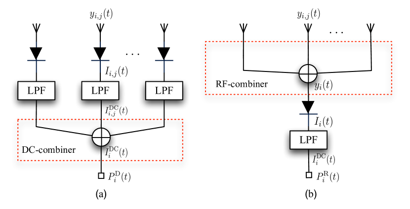
Figure 1: Rectenna array architectures for WPT with $L$ antenna elements; (a) DC-combiner, (b) RF-combiner.

III WPT- Rectenna array configurations

Each terminal is equipped with an array of $L$ elements in order to boost the rectification process. The interconnection of these elements can be performed in the DC or the RF domain.

III-A DC-combiner

In the DC-combiner topology (see Fig. 1(a)), each element operates in an independent way and has its own rectification circuit in order to harvest DC power. The DC currents at the output of each rectifier are combined (simple addition) in order to generate an aggregate DC current, which is the final input to the application. More specifically, the output current of the Schottky diode for the $j$-th antenna element of the $i$-th terminal is given by Shockley’s diode equation [14]

$$I_{i,j}(t) =I_{s}\left(e^{\frac{y_{i,j}(t)}{\mu V_{T}}}-1\right)=I_{s}\sum_{k=1}^{\infty}\left(\frac{y_{i,j}(t)}{\mu V_{T}}\right)^{k},$$ (7)

where $I_{s}$ denotes the reverse saturation current of the diode, $\mu\in[1\;2]$ is an ideality factor (function of the operating conditions and physical contractions), and $V_{T}$ is the thermal voltage; the RHS in (7) is based on the Taylor series expansion of an exponential function. The low pass filter (LPF) at the output of each diode eliminates the harmonic terms ($k>2$) in order to produce a relatively smooth DC current i.e.,

$$I_{i,j}^{\text{DC}}(t)=\frac{I_{s}}{(\mu V_{T})^{2}}d_{i}^{-\alpha}P_{h}|g_{i,j}(t)|.$$ (8)

The DC combiners adds together the $L$ DC components in order to produce a total DC current given by

$$I^{\text{DC}}_{i}(t)=e_{d}\sum_{j=1}^{L}I_{i,j}^{\text{DC}}(t)=\frac{e_{d}I_{s}P_{h}d_{i}^{-\alpha}}{(\mu V_{T})^{2}}\sum_{j=1}^{L}|g_{i,j}(t)|,$$ (9)

where $e_{d}$ denotes the efficiency of the DC combining circuit [8]. The total harvested DC power is a linear function of $I^{\text{DC}}_{i}(t)$ and is written as

$$P_{i}^{\text{D}}(t)=\zeta_{d}I^{\text{DC}}_{i}(t)=\frac{\zeta_{d}e_{d}I_{s}P_{h}d_{i}^{-\alpha}}{(\mu V_{T})^{2}}\sum_{j=1}^{L}|g_{i,j}(t)|^{2},$$ (10)

where $\zeta_{d}$ denotes the conversion efficiency for the DC-combiner topology; we define $G\triangleq\frac{(\mu V_{T})^{2}\sigma^{2}}{\zeta_{d}e_{d}I_{s}P_{h}}$.

III-B RF-combiner

The RF-combiner topology (see Fig. 1(b)) requires only one rectification circuit and combines the antenna inputs in the RF domain. This combination does not requires any intelligence and passively adds the $L$ signals before the rectification process i.e.,

$$y_{i}(t) =e_{r}\sum_{j=1}^{L}y_{i,j}(t)$$

$$=\sqrt{2P_{h}d_{i}^{-\alpha}}e_{r}\Re\left\{e^{\jmath[2\pi ft+\arg{x(t)}]}\sum_{j=1}^{L}|g_{i,j}(t)|e^{j\theta_{i,j}(t)}\right\}$$

$$=\sqrt{2P_{h}d_{i}^{-\alpha}}|c_{i}(t)|e_{r}\cos\left(2\pi ft+\arg{x(t)}+\theta_{i}(t)\right),$$ (11)

where $e_{r}$ denotes the efficiency of the RF combining circuit [8], and $\sum_{j=1}^{L}|g_{i,j}(t)|e^{\jmath\theta_{i,j}(t)}=|c_{i}(t)|e^{j\theta_{i}(t)}$ is a circularly-symmetric complex Gaussian random variable with zero mean and variance $L$. This combined signal is the input to the single Schottky diode; by removing the harmonic terms ($k>2$) through LPF, the DC output and the associated harvested DC power are given by

$$I_{i}^{\text{DC}}(t)=\frac{e_{r}I_{s}P_{h}d_{i}^{-\alpha}}{(\mu V_{T})^{2}}|c_{i}(t)|,$$ (12)

$$P^{\text{R}}_{i}(t)=\zeta_{r}I_{i}^{\text{DC}}(t)=\frac{\zeta_{r}e_{r}I_{s}P_{h}d_{i}^{-\alpha}}{(\mu V_{T})^{2}}|c_{i}(t)|^{2},$$ (13)

where $\zeta_{r}$ is the conversion efficiency for the RF-combiner topology; we define $Y\triangleq\frac{(\mu V_{T})^{2}\sigma^{2}}{\zeta_{r}e_{r}I_{s}P_{h}}$.

IV OBF with $1$-bit feedback

The main problem in the OBF scheme is the assignment of the $M$ beams to $M$ selected terminals; this assignment requires a feedback of the achieved SINR for each beam from all terminals. Based on the received feedback, the AP allocates each beam to the terminal with the highest SINR in order to maximize the sum rate. However, this feedback channel refers to the transmission of a high amount of information, which requires significant system resources such as bandwidth and power. In the considered WPC setup, the terminals have not their own power supply and harvest energy from the PB’s RF signal in order to power their feedback transmission. Due to the small efficiency of the WPT process and the associated doubly near-far problem, we squeeze the feedback channel into $1$-bit [9]. In this case, the main steps of the OBF scheme are summarized as follows:

• The AP broadcasts the $M$ beamforming vectors to the terminals.

• Each terminal measures the SINR for only one beam, randomly assigned to it by the AP. The measured SINR $\Gamma_{i,l}$ is compared to the target SINR value $\Delta$ (function of the quality-of-service); $1$-bit represents whether or not $\Gamma_{i,l}$ is above the threshold.

• Each terminal harvests energy through the rectenna array configuration. If the harvested energy is sufficient (i.e., uplink is not in outage), the terminal transmits $1$-bit feedback to the AP, otherwise remains inactive.

• Based on the received feedback, the AP randomly assigns each beam to one terminal among those who have signaled a SINR on the corresponding beam above the threshold. If none terminal returns a positive feedback for a specific beam, assignment is performed randomly.

IV-A Beam outage probability

A beam is in outage when the achieved SINR is less than a target SINR $\Delta$; we study the outage performance of the $l$-th beam, without loss of generality. In order to derive the outage probability, we firstly state the following proposition.

Proposition 1.

The terminals participating in the beam selection of the $l$-th beam form a homogeneous PPP with an intensity

$$\lambda_{l}^{\text{D}}=\frac{\lambda}{M(\rho^{2}-\xi^{2})}\!\!\sum_{m=0}^{L-1}\!\!\frac{\Gamma\left(m+\frac{1}{\alpha},\!G\xi^{2\alpha}\right)\!-\!\Gamma\left(m+\frac{1}{\alpha},\!G\rho^{2\alpha}\right)}{\alpha G^{\frac{1}{\alpha}}\Gamma(m+1)},$$ (14)

$$\lambda_{l}^{\text{R}}=\frac{\lambda L^{\frac{1}{\alpha}}\left[\Gamma\left(\frac{1}{\alpha},\!\frac{Y}{L}\xi^{2\alpha}\right)-\Gamma\left(\frac{1}{\alpha},\!\frac{Y}{L}\rho^{2\alpha}\right)\right]}{M\alpha(\rho^{2}-\xi^{2})Y^{\frac{1}{\alpha}}},$$ (15)

for the DC-combiner and the RF-combiner, respectively.

Proof.

Since each terminal is preselected to observe a specific beam in a random way, the terminals which observe the $l$-th beam form a PPP $\Phi_{l}$ with intensity $\lambda_{l}=\lambda/M$ (thinning operation [15]).

A terminal becomes active only when the harvested energy at the $t$-th time slot ensures the successful decoding of $1$-bit information in the uplink. This means that the Shannon capacity of the uplink between the terminal and the AP is higher than $1$ bits per channel use. For the $i$-th terminal, this condition is expressed as

$$\log_{2}\left(1+\frac{P_{i}^{\mathcal{Q}}(t)}{d_{i}^{\alpha}\sigma^{2}}\right)\geq 1\Rightarrow P_{i}^{\mathcal{Q}}(t)\geq d_{i}^{\alpha}\sigma^{2},$$ (16)

where $\mathcal{Q}\in\{\text{D,R}\}$. For the DC-combiner topology, the probability that the $i$-th terminal is idle can be written as

$$\Pi^{\text{D}} =\mathbb{P}\{P_{i}^{\text{D}}(t)<d_{i}^{\alpha}\sigma^{2}\}\;=\mathbb{P}\left\{Z<Gd_{i}^{2\alpha}\right\}$$

$$=\mathbb{E}\left[\frac{\gamma(L,Gd_{i}^{2\alpha})}{\Gamma(L)}\right]\;=\int_{0}^{2\pi}\int_{\xi}^{\rho}\frac{\gamma(L,Gr^{2\alpha})}{\Gamma(L)}f_{d}(r)rdrd\theta$$

$$=1-\frac{2}{\rho^{2}-\xi^{2}}\sum_{m=0}^{L-1}\frac{G^{m}}{\Gamma(m+1)}\int_{\xi}^{\rho}e^{-Gr^{2\alpha}}r^{2\alpha m+1}dr$$ (17a)

$$=1\!-\!\frac{1}{\alpha(\rho^{2}-\xi^{2})G^{\frac{1}{\alpha}}}\sum_{m=0}^{L-1}\frac{\Gamma\left(m+\frac{1}{\alpha},\!G\xi^{2\alpha}\right)\!-\!\Gamma\left(m+\frac{1}{\alpha},\!G\rho^{2\alpha}\right)}{\Gamma(m+1)},$$ (17b)

where $Z\triangleq\sum_{j=1}^{L}|g_{i,j}|^{2}$ is a central chi-square random variable with $2L$ degrees of freedom; the cumulative distribution function (CDF) of $Z$ is $F_{Z}(x)=\gamma(L,x)/\Gamma(L)$, where $\gamma(a,x)$ denotes the lower incomplete gamma function [16] and $\Gamma(x)$ denotes the Gamma function; $f_{d}(x)=1/\pi(\rho^{2}-\xi^{2})$ denotes the probability density function of each point in $\mathcal{B}$; (17a) is based on [16, 8.352] and (17b) uses the expressions in [16, 3.381].

For the RF-combiner topology, the probability that the $i$-th terminal is not able to return a feedback is written as

$$\Pi^{\text{R}} =\mathbb{P}\{P_{i}^{\text{R}}(t)<d_{i}^{\alpha}\sigma^{2}\}\;=\mathbb{P}\{Z_{1}<Yd_{i}^{2\alpha}\}$$

$$=\mathbb{E}\left[1-e^{-\frac{Yd_{i}^{2\alpha}}{L}}\right]\;=1-\int_{0}^{2\pi}\int_{\xi}^{\rho}e^{-\frac{Y}{L}r^{2\alpha}}f_{d}(r)rdrd\theta$$

$$=1-\frac{L^{\frac{1}{\alpha}}}{\alpha(\rho^{2}-\xi^{2})}\frac{\Gamma\left(\frac{1}{\alpha},\!\frac{Y}{L}\xi^{2\alpha}\right)-\Gamma\left(\frac{1}{\alpha},\!\frac{Y}{L}\rho^{2\alpha}\right)}{Y^{\frac{1}{\alpha}}},$$ (18)

where $Z_{1}\triangleq|c_{i}(t)|^{2}$ is an exponential random variable with parameter $1/L$ and a CDF equal to $F_{Z_{1}}(x)=1-e^{-x/L}$.

By using thinning transformation, the terminals which feed $1$-bit for the $l$-th beam form a homogeneous PPP $\Phi_{l}^{\mathcal{Q}}$ with intensity $\lambda_{l}^{\mathcal{Q}}=\lambda_{l}(1-\Pi^{\mathcal{Q}})$. Substituting the above expressions, the proposition is then proved. ∎

According to the proposed OBF scheme, for the $l$-th beam, an outage event occurs when none terminal returns a positive feedback for the achieved beam SINR and the link (if any) between the AP and the random selected terminal is in outage. The case where all terminals return a negative feedback is equivalent to the case where the maximum achieved beam SINR (among the terminals which feed $1$-bit) is lower than the requested threshold. For the beam outage probability, we state Theorem 1.

Theorem 1.

The beam outage probability for the $l$-th beam and the $\mathcal{Q}$ combiner ($\mathcal{Q}\in\{\rm{D,R}\}$) is given by

$$P_{\rm{out}}^{\mathcal{Q}}=e^{-\lambda_{l}^{\mathcal{Q}}\pi(\rho^{2}-\xi^{2})(1-F_{\Gamma}(\Delta))}\bigg{[}e^{-(\frac{\lambda}{M}-\lambda_{l}^{\mathcal{Q}})\pi(\rho^{2}-\xi^{2})}+\left(1-e^{-(\frac{\lambda}{M}-\lambda_{l}^{\mathcal{Q}})\pi(\rho^{2}-\xi^{2})}\right)F_{\Gamma}(\Delta)\bigg{]},$$ (19)

where $F_{\Gamma}(x)$ is defined in (21).

Proof.

The CDF of the observed beam SINR for a given path-loss value $d$ is written as [2]

$$F_{\Gamma}(x|d_{i}=d)=\left[1-\frac{e^{-\frac{xd^{\alpha}}{P_{t}}}}{(x+1)^{M-1}}\right]^{N},$$ (20)

with expectation over $d$, the observed beam SINR has a CDF given by

$$F_{\Gamma}(x) =\int_{0}^{2\pi}\int_{\xi}^{\rho}\left[1-\frac{e^{-\frac{xr^{\alpha}}{P_{t}}}}{(x+1)^{M-1}}\right]^{N}f_{d}(r)rdrd\theta$$

$$\;\;=1+\frac{2}{\alpha(\rho^{2}-\xi^{2})}\left(\frac{P_{t}}{x}\right)^{\frac{2}{\alpha}}\sum_{m=1}^{N}\binom{N}{m}\frac{(-1)^{m}}{m^{\frac{2}{\alpha}}(x+1)^{m(M-1)}}$$

$$\;\;\;\;\times\left[\Gamma\left(\frac{2}{\alpha},\frac{xm\xi^{\alpha}}{P_{t}}\right)-\Gamma\left(\frac{2}{\alpha},\frac{xm\rho^{\alpha}}{P_{t}}\right)\right],$$ (21)

where (21) uses the binomial theorem as well as the expressions in [16, 3.381]. On the other hand, let’s assume that $n$ terminals are able to return a feedback to the AP. By using high order statistics, the CDF of the maximum beam SINR i.e., $\Gamma_{l}^{*}=\max_{1\leq i\leq n}\Gamma_{i,l}$, conditioning on $n$ and path-loss values is written as

$$F_{\Gamma^{*}}(x|n,d_{1},\ldots,d_{n})=\prod_{i=1}^{n}F_{\Gamma}(x|d_{i}).$$ (22)

With expectation over the path-loss values, we have

$$F_{\Gamma^{*}}(x|n)\!\!=\!\!\left[\int_{0}^{2\pi}\!\!\!\!\int_{\xi}^{\rho}F_{\Gamma}(x|r)f_{d}(r)drd\theta\right]^{n}\!\!\!=[F_{\Gamma}(x)]^{n}.$$ (23)

The beam outage probability for the $l$-th beam and the $\mathcal{Q}$ combiner is expressed as

$$P_{\text{out}}^{\mathcal{Q}} =\mathbb{E}\{\Gamma_{l}^{*}<\Delta|\Phi_{l}^{\mathcal{Q}}\}\mathbb{E}\{\Gamma_{l}<\Delta|\overline{\Phi_{l}^{\mathcal{Q}}}\}$$

$$=\sum_{n=0}^{\infty}\mathbb{P}\{\Gamma^{*}_{l}<\Delta|n\}\mathbb{P}\{N_{\Phi_{l}^{\mathcal{Q}}}(\mathcal{B})=n\}$$

$$\times\left[\mathbb{P}\{N_{\overline{\Phi_{l}^{\mathcal{Q}}}}(\mathcal{B})=0\}+\mathbb{P}\{N_{\overline{\Phi_{l}^{\mathcal{Q}}}}(\mathcal{B})>0\}\mathbb{P}\{\Gamma_{l}<\Delta\}\right],$$ (24)

with

$$\mathbb{P}\big{\{}N_{\overline{\Phi_{l}^{\mathcal{Q}}}}(\mathcal{B})=0\big{\}}=e^{-\overline{\lambda_{l}^{\mathcal{Q}}}|\mathcal{B}|},$$ (25)

$$\sum_{n=0}^{\infty}\mathbb{P}\{\Gamma^{*}_{l}<\Delta|n\}\mathbb{P}\{N_{\Phi_{l}^{\mathcal{Q}}}(\mathcal{B})=n\}$$

$$=\sum_{n=0}^{\infty}\frac{e^{-\lambda_{l}^{\mathcal{Q}}|\mathcal{B}|}\left(\lambda_{l}^{\mathcal{Q}}|\mathcal{B}|F_{\Gamma}(\Delta)\right)^{n}}{n!}=e^{-\lambda_{l}^{\mathcal{Q}}|\mathcal{B}|(1-F_{\Gamma}(\Delta))},$$ (26)

where $\overline{\Phi_{l}^{\mathcal{Q}}}$ denotes the complementary homogeneous PPP with intensity $\overline{\lambda_{l}^{\mathcal{Q}}}\triangleq\lambda_{l}\Pi^{\mathcal{Q}}$, which is formed by the terminals that are not able to return $1$-bit feedback; $N_{\mathcal{Z}}(\mathcal{B})$ denotes the number of terminal in $\mathcal{B}$ for a PPP $\mathcal{Z}$, and $|\mathcal{B}|=\pi(\rho^{2}-\xi^{2})$. By substituting (21), (25), (26) into (24), we prove the statement. ∎

Remark 1.

For $P_{t},P_{h}\rightarrow\infty$, the beam outage probability for both combination schemes asymptotically converges to

$$P_{\rm{out}}=e^{-\frac{\lambda}{M}\pi(\rho^{2}-\xi^{2})(1-F_{\Gamma}^{\infty}(\Delta))},$$ (27)

where $F_{\Gamma}^{\infty}(x)=[1-1/(x+1)^{M-1}]^{N}$.

Proof.

For $P_{t},P_{h}\rightarrow\infty$, all the terminals successfully transmit $1$-bit feedback and thus $\lambda_{l}^{\mathcal{Q}}\rightarrow\lambda_{l}$. Remark 1 can be straightforwardly obtained from $P_{\text{out}}=\mathbb{E}\{\Gamma_{l}^{*}<\Delta|\Phi_{l}\}$. ∎

V Numerical results and discussion

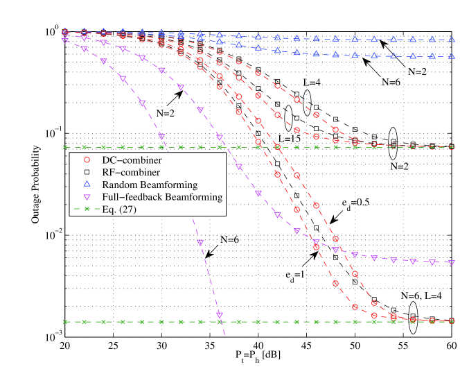
Figure 2: Outage Probability versus the transmit power with $P_{t}=P_{h}$; $\xi=2$ m, $\rho=10$ m, $I_{s}=1$ mA, $\mu=2$, $V_{T}=28.85$ mV, $\zeta_{d}=\zeta_{r}=0.9$, $e_{r}=1$, $e_{d}=\{1,0.5\}$, $\sigma^{2}=-10$ dBm, $\alpha=3$, $M=2$, $N=\{2,6\}$, $L=\{4,15\}$, $\Delta=10$ dB, and $\lambda=0.1$; the dashed lines represent the theoretical results.

Fig. 2 plots the beam outage probability versus the transmit power for both RF/DC combination schemes; the random beamforming (no feedback) and the full-feedback OBF [2] (terminals feed SINR information for all beams) are used as benchmarks. The first main observation is that the proposed $1$-bit OBF significantly outperforms random assignments. The associated gain increases as the number of receive antennas $N$ increases (receive diversity). On the other hand, it can be seen that the beam outage probability performance is improved as $L$ increases for moderate values of $P_{h}$ (see the case with $N=2$). As the size of the rectenna array increases, the terminals harvest more energy and therefore return $1$-bit feedback with a higher probability.

As for the combination topologies, it can be seen that the DC-combiner outperfoms the RF-combiner for the ideal case with $e_{d}=e_{r}=1$ e.g., gain of $3$ dB for $P_{t}=50$ dB and $N=6$. However, the performance of the combination schemes and their suitability highly depend on the quality of the associated combining circuits. We can observe that the RF-combiner achieves a lower outage probability than the DC-combiner when $e_{r}=1$ and $e_{d}=0.5$ (see the case with $N=6$). Therefore, the designer should carefully take into account the insertion losses of the combining circuits in order to select the best configuration. For high values of $P_{t},P_{h}$ both combination schemes converge to the same outage probability floor, in accordance to Remark 1.

References

• [1] M. Sharif and B. Hassibi, β€œOn the capacity of MIMO broadcast channels with partial side information,” IEEE Trans. Inf. Theory, vol. 51, pp. 506–522, Feb. 2005.
• [2] M. -O. Pun, V. Koivunen, and H. V. Poor, β€œPerformance analysis of joint opportunistic scheduling and receiver design for MIMO-SDMA downlink systems,” IEEE Trans. Comm., vol. 59, pp. 268–280, Jan. 2011.
• [3] T. Samarasinghe, H. Inaltekin, and J. S. Evans, β€œOn the outage capacity of opportunistic beamforming with random user locations,” IEEE Trans. Comm., vol. 62, pp. 3015–3026, Aug. 2014.
• [4] R. Zhang and C. K. Ho, β€œMIMO broadcast for simultaneous wireless information and power transfer,” IEEE Trans. Wireless Comm., vol. 12, pp. 1989-2001, May 2013.
• [5] H. Ju and R. Zhang, β€œThroughput maximization in wireless powered communication networks,” IEEE Trans. Wireless Comm., vol. 13, pp. 418–428, Jan. 2014.
• [6] I. Krikidis, S. Timotheou, S. Nikolaou, G. Zheng, D. W. K. Ng, and R. Schober, β€œSimultaneous wireless information and power transfer in modern communication systems”, IEEE Comm. Mag., vol. 52, pp. 104-110, Nov. 2014.
• [7] M. Xia and S. Aissa, β€œOn the efficiency of far-field wireless power transfer,” IEEE Trans. Sign. Proc., vol. 63, pp. 2835–2847, June 2015.
• [8] U. Olgun, C. -C. Chen, and J. L. Volakis, β€œInvestigation of rectenna array configurations for enhanced RF power harvesting,” IEEE Ant. Wireless Prop. Lett., vol. 10, pp. 262–265, 2011.
• [9] J. Diaz, O. Simeone, and Y. Bar-Ness, β€œHow many bits of feedback is multiuser diversity worth in MIMO downlink?,” in Proc. IEEE Symp. Spread Spec. Tech. Appl., Manaus, Brazil, Aug. 2006, pp. 505–509.
• [10] A. A. Nasir, X. Zhou, S. Durrani, and R. A. Kennedy, β€œRelaying protocols for wireless energy harvesting and information processing,” IEEE Trans. Wireless Comm., vol. 12, pp. 3622–3636, July 2013.
• [11] Z. Ding and H. V. Poor, β€œCooperative energy harvesting networks with spatially random users,” IEEE Sign. Proc. Lett., vol. 20, pp. 1211-1214, Dec. 2013.
• [12] M. Kobayashi, N. Jindal, and G. Caire, β€œTraining and feedback optimization for multiuser MIMO downlink,” IEEE Trans. Comm., vol. 59, pp. 2228–2240, Aug. 2011.
• [13] C. -F. Liu and C. -H. Lee, β€œInformation and power transfer under MISO channel with finite-rate feedback,” in Proc. IEEE Global Comm. Conf., Atlanta, USA, Dec. 2013, pp. 2519–2523.
• [14] R. L. Boylestad and L. Nashelsky, Electronic devices and circuit theory, 11-th Ed, Pearson Ed., 2013.
• [15] M. Haenggi, Stochastic geometry for wireless networks, Cambridge Uni. Press, 2013.
• [16] I. S. Gradshteyn and I. M. Ryzhik, Table of integrals, series, and products, Elsevier, 2007.