The geometry of coexistence in large ecosystems

Abstract

The role of species interactions in controlling the interplay between the stability of an ecosystem and its biodiversity is still not well understood. The ability of ecological communities to recover after a small perturbation of the species abundances (local asymptotic stability) has been well studied, whereas the likelihood of a community to persist when the interactions are altered (structural stability) has received much less attention. Our goal is to understand the effects of diversity, interaction strenghts and ecological network structure on the volume of parameter space leading to feasible equilibria, i.e., ones in which all populations have positive abundances. We develop a geometrical framework to study the range of conditions necessary for feasible coexistence in both mutualistic and consumer–resource systems. Using analytical and numerical methods, we show that feasibility is determined by just a handful of quantities describing the interactions, yielding a nontrivial complexity–feasibility relationship. Analyzing more than 100 empirical networks, we show that the range of coexistence conditions in mutualistic systems can be analytically predicted by means of a null model of random interactions, whereas food webs are characterized by smaller coexistence domains than those expected by chance. Finally, we characterize the geometric shape of the feasibility domain, thereby identifying the direction of perturbations that are more likely to cause extinctions. Interestingly, the structure of mutualistic interactions leads to very heterogeneous responses to perturbations, making those systems more fragile than expected by chance.

Natural populations are faced with constantly varying environmental conditions. Environmental conditions affect physiological parameters (e.g., metabolic rates  Gillooly2001 ) as well as ecological ones (e.g., the presence and strength of interactions between populations Walther2002 ; Tylianakis2008 ; Harmon2009 ; Tylianakis2010 ). Therefore in order to persist, ecological communities necessarily need, at the very least, to be able to cope with small environmental changes. Mathematically, this translates into an argument on the robustness of the qualitative behavior of an ecological dynamical system: to guarantee robust coexistence, a model describing an ecological community needs at least to be (qualitatively) insensitive to small perturbations of the parameters  Meszenaetal2006 ; Barabasetal2014ELE . This notion has been formalized in the measure of robustness Barabas2012 or “structural stability” Rohr2014 , expressed as the volume of the parameter space resulting in the coexistence of all populations in a community.

While the local asymptotic stability (the ability to recover after a small change in the population abundances) of ecological communities has been studied in small May1975 and large May1972 ; Allesina2012 ; suweis2014disentangling ; Allesina2015a systems, the study of structural stability (i.e., the ability of a community to retain the same dynamical behavior if conditions are slightly altered)—despite being proposed early on as a key feature in the context of the diversity-stability debate MacArthur1955 ; GILPIN1975 ; ROBERTS1974 ; Goh1977a —has historically been restricted to the case of small communities, with the first studies of larger communities appearing only recently Rohr2014 ; Saavedra2016 , and—because of mathematical limitations—dealing exclusively with the case of large mutualistic communities. Studies of structural stability have so far focused on the effect of ecological network structure (who interacts with whom) on the volume of parameter space leading to feasible equilibria, in which all populations have positive abundances.

Here we develop a geometrical framework for studying the feasibility of large ecological communities. We overcome the limitations that have hitherto prevented the study of consumer-resource networks, thereby providing a unified view of feasibility in ecological systems. Using a random matrix approach (which helped identify main drivers of local asymptotic stability), we pinpoint the key quantities controlling the volume of parameter space leading to feasible communities, as well as its sensitivity to changes in these parameters. We then contrast these expectations for randomly connected systems with simulations on structured empirical networks, quantifying the effects of network structure on feasibility.

Theoretical framework

For simplicity, we consider a community composed of $S$ species whose dynamics is determined by a system of autonomous ordinary differential equations:

$$\frac{dn_{i}}{dt}=n_{i}\left(r_{i}+\sum_{j=1}^{S}A_{ij}n_{j}\right)\ ,$$ (1)

where $n_{i}$ is the density of population $i$, $r_{i}$ is its intrinsic growth rate, and $A_{ij}$ (which in principle could depend on $\boldsymbol{n}$; see Supplementary Information) measures the interaction strength between population $i$ and $j$. A fixed point $\boldsymbol{n}^{\ast}$ (i.e., a vector of densities making the right side of each equation zero) is feasible if $n_{i}^{\ast}>0$ for every population. A fixed point is locally asymptotically stable if, following any sufficiently small perturbation of the densities, the system returns to a small vicinity of the fixed point. The fixed point is globally asymptotically stable if the system eventually return to it, starting from any positive initial condition within a finite domain. A system with a fixed point is structurally stable if, following a sufficiently small change in the growth rates $r_{i}$, the new fixed point is still feasible and stable.

To study the range of conditions leading to stable coexistence, we need to disentangle feasibility and local stability. This problem is well discussed in Rohr et al. Rohr2014 , where it was solved for the case of one possible parameterization of mutualistic interactions. If $\boldsymbol{A}$ is diagonally stable or Volterra dissipative (i.e., there exists a positive diagonal matrix $\boldsymbol{D}$ such that $\boldsymbol{D}\boldsymbol{A}+\boldsymbol{A}^{T}\boldsymbol{D}$ is stable), then any feasible fixed point is globally stable Volterra1931 ; Goh1977 . Unfortunately, a general characterization of this class of matrices is unknown  Logofet2005 . We proceeded therefore by considering only the matrices such that all the eigenvalues of $\boldsymbol{A}+\boldsymbol{A}^{T}$ are negative (i.e., the matrix $\boldsymbol{A}$ is negative definite in a generalized sense  Johnson1970 , corresponding to $\boldsymbol{D}$ being equal to the identity matrix; see Methods). This choice reduces the number of parameterizations one can analyze, as not all the diagonally stable matrices are negative definite. However, as shown in the Supplementary Information, only very few parameter combinations are excluded from this set. Moreover, the effects of negative definitness are well–studied for random matrices  Tang2014 , and by using it we can extend the study of feasibility to any ecological network, including food webs.

Our goal is to measure the fraction of growth rate combinations, out of all possible combinations, that lead to the coexistence of all $S$ populations. Since we can separate stability and feasibility, we only need to find those $r_{i}$ leading to feasible fixed points, and the condition above ensures that these will be globally stable. As pointed out before Rohr2014 , the problem is not to find a particular set of $r_{i}$ leading to coexistence, but rather to measure how flexibly one may choose these rates. As shown in Fig. 1, this quantity–indicated by $\Xi$ henceforth–can be thought of as a volume, or more precisely a solid angle, in the space of growth rates Svirezhev1978 (see Methods).

To calculate $\Xi$, one might naively wish to perform direct numerical computation of the fraction of growth rates leading to a feasible equilibrium. While a direct calculation is viable when $S$ is sufficiently small, this procedure becomes extremely inefficient for large $S$ Rohr2014 . In the Supplementary Information we introduce a method that can be used to efficiently calculate $\Xi$ with arbitrary precision, even for large $S$. Using this method, we can accurately measure the size of the feasibility domain, with larger values of $\Xi$ corresponding to larger proportions of conditions (intrinsic growth rates) compatible with stable coexistence. For reference, we normalize $\Xi$ so that $\Xi=1$ when populations are self–regulated and not interacting (Methods), i.e., when the interaction matrix $\boldsymbol{A}$ is a negative diagonal matrix, and thus Eq. 1 simplifies to $S$ independent logistic equations.

Results

Feasibility is universal for random matrices.

May’s seminal work May1972 pioneered the use of random matrices as a reference, or null model, of ecological interactions. A particularly interesting feature of random matrices is that the distribution of their eigenvalues (determining local stability) is universal Allesina2015 . This means that local stability depends on just a few, coarse–grained properties of the matrix (i.e., the number of species and the first few moments of the distribution of interaction strengths) and not on the finer details (e.g., the particular distribution of interaction strengths; see Supplementary Information). In fact, these moments can be combined into just three parameters: $E_{1}$, $E_{2}$, and $E_{c}$ (Methods). Together with $S$, they completely determine local asymptotic stability.

We tested whether universality also applies to feasibility. We considered different random matrix ensembles obtained for different connectance values and distributions from which the matrix entries were drawn, but with constant values of $S$ and of $E_{1}$, $E_{2}$, and $E_{c}$. We then checked whether the size $\Xi$ of the feasibility domain depended only on these four quantities or also on finer details. Surprisingly, we found that the feasibility of random matrices is also universal (Methods and Supplementary Information). Two very different (random) ecosystems, with completely different interaction types and distributions of interaction strengths, but having the same number of species $S$ and the same $E_{1}$, $E_{2}$, and $E_{c}$, have the same $\Xi$ in the large $S$ limit. This result has important theoretical implications, as it indicates those moments as the drivers of feasibility, but also very practical consequences, namely that the parameter space one needs to explore is dramatically reduced.

An analytical complexity–feasibility relationship

The universality of $\Xi$ suggests that it is amenable to analytical treatment. As explained in the Supplementary Information and shown in Fig. 2, when the mean and variance of interaction strengths are not too large (Supplementary Information), we are able to derive the following approximation for $\Xi$ for random interaction matrices $\boldsymbol{A}$:

$$\Xi\sim\Bigl{(}1+\frac{1}{\pi}\frac{E_{1}(2d-SE_{1})}{d-SE_{1}^{2}}\Bigr{)}^{S}\ ,$$ (2)

where $S$ is is the number of species, $d$ is the mean of $\boldsymbol{A}$’s diagonal entries, and $E_{1}=C\mu$, the product of the connectance $C$ and the average interaction strength $\mu$ (see Methods). A more accurate formula is presented in the Supplementary Information.

In analogy with the celebrated result of May May1972 connecting stability and complexity, Eq. 2 can be considered as a complexity–feasibility relationship. While in May’s scenario and in its generalizations Allesina2012 the effect of complexity and diversity on stability is always detrimental, it does depend on the interaction type in the case of feasibility. Given that $d$ is negative by construction (Supplementary Information), having more species or connections can either increase ($E_{1}>0$) or shrink ($E_{1}<0$) the size of the feasibility domain, as a function of the sign of interaction strenghts (see Fig. 2). It is important to stress that we computed $\Xi$ under the assumption of $\boldsymbol{A}$ being negative definite. When we consider how $\Xi$ depends on $S$ and other parameters, we need to take into account the conditions making the matrix negative definite (see Methods and Supplementary Information). In the case of positive interaction strengths, this condition is $d+SC\mu<0$, implying an upper bound for $\mu$ that depends on $S$.

Our analytical formula predicts feasibility of empirical mutualistic networks and overestimates that of food webs

Having explored the feasibility of random networks, we proceed to investigate the effects of incorporating empirical network structure. Ecological networks are in fact non–random Cohenetal1990 ; Williams2000 ; Bascompte2003 , and many studies have hypothesized that the structure of interactions could increase the likelihood of coexistence Bascompte2006 ; Bastolla2009 ; Thebault2010 . Having an analytical prediction for random matrices, we can study whether it predicts the size of the feasibility domain for empirical networks as well. Fig. 2 shows the simulated values of $\Xi$ for 89 mutualistic networks and 15 food webs (Supplementary Information), parameterized multiple times and compared with our analytical approximation (see Methods). We find that $\Xi$ of empirical mutualistic networks is well predicted by our formula, while it overestimates the feasibility domain of food webs, indicating that their non–random structure has a strong negative effect on feasibility.

In the Supplementary Information, we compare the effect of the empirical structure of mutualistic networks with randomizations, by controlling for the interaction strengths. We show that, in the absence of variability in interaction strengths, the structure of empirical mutualistic networks has a positive effect on feasibility, which is strongly reduced when interaction strengths are allowed to vary. While this effect of empirical mutualistic networks is statistically significant, its effect on $\Xi$ is negligible compared to the effect of mean interaction strengths, and can only be detected by controlling very precisely for interaction strengths (see Supplementary Information). On a broader scale, as shown in Fig. 2, the size of the feasibility domain of empirical networks is well predicted by our analytical formula.

On the other hand, the negative effect of food web structure on $\Xi$ is substantial. In the Supplementary Information we compare each network with randomizations and also with predictions of the cascade model Cohenetal1990 , which has recently been shown to predict well the stability of empirical food webs Allesina2015a . By analyzing different parameterizations we found that the feasibility domain of empirical structures is consistently and significantly smaller than that of both the randomizations and the cascade model. For most of the webs, the prediction obtained from the cascade model is better than that of randomizations, suggesting that the directionality of empirical webs plays a role in reducing feasibility, with other properties of the structure of empirical networks also contributing significantly to feasibility.

The shape of the feasibility domain carries information on the response to perturbations, and can be analytically predicted for random interactions

So far, we have focused on the volume of the parameter space resulting in feasiblity. However, two systems having the same $\Xi$ can still have very different responses to parameter perturbations, just as two triangles having the same area need not to have sides of the same length (Fig. 1). The two extreme cases correspond to a) an isotropic system in which, if we start at the barycenter of the feasibility domain, moving in any direction yields roughly the same effect (equivalent to an equilateral triangle); b) anisotropic systems, in which the feasibility domain is much narrower in certain directions than in others (as in a scalene triangle). For our problem, the domain of growth rates leading to coexistence is—once the growth rates are normalized—the $(S-1)$–dimensional generalization of a triangle on a hypersphere. For $S=3$, this domain is indeed a triangle lying on a sphere as shown in Fig. 1. If all the $S(S-1)/2$ sides of this (hyper–)triangle are about the same length, then different perturbations will have similar effects on the system. On the other hand, if some sides are much shorter than others, then there will be changes of conditions which will more likely impact coexistence than others. We therefore consider a measure of the heterogeneity in the distribution of the side lengths (Fig. 1 and Supplementary Information). The larger the variance of this distribution, the more likely it is that certain perturbations can destroy coexistence, even when $\Xi$ is large and the perturbation small. This way of measuring heterogeneity is particularly convenient because it is independent of the initial conditions. Moreover, the length of each side can be directly related to the similarity between the corresponding pair of species (Supplementary Information), drawing a strong connection between the parameter space allowing for coexistence and the phenotypic space. As in the case of $\Xi$, this measure is a function of the interaction matrix and corresponds to a geometrical property of the coexistence domain.

While $\Xi$ is a universal quantity for random networks, the distribution of side lengths is not: it depends on the full distribution of interaction strengths (Supplementary Information). On the other hand, as shown in the Supplementary Information, it is possible to compute it analytically in full generality, i.e., for any distribution of interaction strengths and any interaction types. In particular we are able to obtain an expression for its mean and variance, which depend only on $S$, $E_{1}$, $E_{2}$, and $E_{c}$ (Supplementary Information). Fig. 3 shows that the analytical formula, in the case of random $\boldsymbol{A}$, matches the observed mean and variance of side lengths of random networks perfectly.

Empirical network structures correspond to more heterogeneous shapes

As we have done for $\Xi$, we can now test how non–random empirical network topologies influence the distribution of side lengths. Fig. 3 shows that empirical food webs and, in particular, empirical mutualistic networks display a much larger variation in side lengths than expected by chance. This result is particularly relevant, indicating that even if the feasibility domains of empirical mutualistic networks are larger than those of random networks, their shapes are less regular than expected by chance, and thus we expect perturbations in certain directions to quickly lead out of the feasible domain of growth rates.

Discussion

A classic problem in mathematical ecology is determining the response of systems to perturbations of model parameters. In the community context, one important application is getting at the range of parameters allowing for species coexistence ArmstrongMcGehee1976 ; ArmstrongMcGehee1980 ; Abrams1983 . Several methods exist for evaluating this range Yodzis1988 ; Dambacheretal2002 ; Aufderheideetal2013 ; Barabasetal2014ELE , but they either rely on raw numerical techniques, or else can only evaluate system response to small parameter perturbations. Here, in the context of the general Lotka–Volterra model, we have given a method for the global assessment of all combinations of species’ intrinsic growth rates compatible with coexistence—what we have called the domain of feasibility. Our geometrical approach can determine not only the total size of the feasibility domain, but also its shape: it is always a simply connected domain forming a convex polyhedral cone whose side lengths can be evaluated from the interaction matrix. Applying our method to empirical interaction networks, we were able to characterize the region of parameter space compatible with coexistence; the importance of this kind of information is underlined by a rapidly changing environment that is expected to cause substantial shifts in the parameters influencing these systems.

The geometrical framework we employed, pioneered by Svirezhev and Logofet Svirezhev1978 , allows for the formulation of a complexity–feasibility relationship. In analogy with the celebrated complexity–stability relationship, it relates the size of the feasibility domain with diversity, connectance and interaction strengths of a random interacting community. While communities are not random, this relationship sets a null expectation for the scaling of the proportion of feasible conditions. We obtain that the mean of interaction strengths sets the behavior of feasibility with the number of species. If the mean is negative (e.g., in case of competition or predation with limited efficiency), the larger the system is, the smaller is the set of conditions leading to coexistence, while for positive mean (e.g., in the case of mutualism) the converse is true.

Several recent works have studied the effect of network structure on coexistence in species–rich communities, with contrasting results  Bascompte2006 ; Bastolla2009 ; Thebault2010 ; Suweis2013 ; Rohr2014 . Here we have shown that the fraction of conditions compatible with coexistence is mainly determined by the number and the mean strength of interactions. In terms of network properties, the relevant quantity is the connectance, with other properties (e.g., nestedness or degree distribution) having minimal effects. In particular, once the connectance and mean interaction strength are fixed, the matrices built using empirical mutualistic networks have feasibility domains very similar to that expected for the random case, as was also observed previously in a similar context James2012 .

The empirical network structure of mutualistic networks has a statistically significant effect on the size of the feasibility domain (see Supplementary Information). Whether this effect is ecologically relevant depends on the specific application at hand. For instance, the effect of structure could be neglected to quantify how the feasibility domain would change if a fraction of pollinators went extinct, and it could be evaluated using our analytical result. In contexts where the interaction strengths are strongly constrained, structure would play an important role. Our method provides, in this respect, a direct way of quantifying the importance of different factors, disentangling the way different interaction properties affect feasibility.

For mutualistic interaction networks, our results clearly show which properties determine the global health of the community, and therefore indicate which properties should be measured in the field. While not observing a link or measuring a wrong interaction coefficient could have strong effects on ecosystem dynamics, they have very little effect on how the community copes with environmental perturbations and how likely extinctions are BarabasAllesina2015 . The major role is played by corse–grained statistical properties of the interactions, such as connectance or the mean and variance of the interaction strengths.

For food webs, on the other hand, empirical systems tend to have feasibility domains smaller than either their random counterparts or models conserving the directionality of interactions (cascade model). It is an open question which properties of real food webs are responsible for restricting the feasibility domain in this way. A possible candidate is the group structure observed in food webs allesina2009food , corresponding to larger similarity of how certain species interact with the rest of the system than expected by chance, which in turn reduces the size of the feasibility domain (see Supplementary Information).

These results parallel those for the distribution of the side lengths of the convex polyhedral cone delimiting the feasibility domain. The variance of side lengths for empirical structures is much higher than in random networks. This implies that even if the total size of the feasibility domain is large, it will have a distorted shape that is very stretched along some directions and shortened along others (Fig. 1). Consequently, it will be possible to find parameter perturbations of small magnitude that will drive the system outside its feasibility domain  Suweis2015 .

We have shown that each side of the feasibility domain corresponds to a pair of species, with the length determined by how similarly the two species interact with the rest of the system. As two species interact more and more similarly (i.e., have a larger niche overlap), the corresponding side becomes shorter and shorter, which in turns means greater sensitivity to parameter perturbations. Consistently with earlier results Barabas2012 ; Barabasetal2014ELE , this fact establishes a relationship between niche overlap and the range of conditions that lead to coexistence: greater niche overlap means a more restricted parameter range allowing for coexistence, irrespective of the details of the interactions.

These differences between the size and shape of the feasibility domain shed light on the contrasting results obtained in the past on the effect of network structure on persistence Bascompte2006 ; Bastolla2009 ; Thebault2010 ; James2012 ; Suweis2013 ; Suweis2015 . Most of these studies rely on numerical integration, and therefore strongly depend on initial conditions. Given the difference in the shape of the feasibility domains of random and empirical networks, different initial conditions and their perturbations could result in markedly different outcomes: the feasibility domain could appear to be large or small depending on the direction in which perturbations are made.

Methods

Disentangling stability and feasibility

From Eq. 1, a feasible fixed point, if it exists, is given by the solution of

$$\sum_{j=1}^{S}A_{ij}n^{\ast}_{j}=-r_{i}\ ,$$ (3)

where the asterisk denotes equilibrium values. A fixed point is locally asymptotically stable if all eigenvalues of the community matrix

$$M_{ij}=n_{i}^{\ast}A_{ij}$$ (4)

have negative real parts. As discussed in the Supplementary Information, if $\boldsymbol{A}$ is diagonally stable or Volterra dissipative (i.e., there exists a positive diagonal matrix $\boldsymbol{D}$ such that $\boldsymbol{D}\boldsymbol{A}+\boldsymbol{A}^{T}\boldsymbol{D}$ is stable), then a feasible fixed point is globally stable in $\mathbb{R}_{+}$.

A general characterization of diagonally stable matrices is unknown for $S>3$  Logofet2005 . There exist algorithms  Redheffer1985 that reduce the problem of determining if a $S\times S$ matrices is diagonally stable into two simultaneous problems of $(S-1)\times(S-1)$ matrices. While this method can be efficiently used to determine the diagonal stability of $4\times 4$ matrices, it becomes computationally intractable for large $S$.

A matrix $\boldsymbol{A}$ is negative definite if

$$\sum_{j}x_{i}A_{ij}x_{j}<0\ ,$$ (5)

for any non–zero vector $\boldsymbol{x}$. A necessary and sufficient condition for a real matrix $\boldsymbol{A}$ to be negative definite is that all the eigenvalues of $\boldsymbol{A}+\boldsymbol{A}^{T}$ are negative Johnson1970 . A negative definite matrix is also diagonally stable, as the condition for diagonal stability holds with $\boldsymbol{D}$ being the identity matrix. Since it is extremely simple to verify this condition and it has been characterized for random matrices, we will study feasibility of negative definite matrices. In the Supplementary Information we show that with this choice we are excluding only a small region of the parameter space.

Size of the feasibility domain

The quantity $\Xi$ is the proportion of intrinsic growth rates leading to feasible equilibria. While a more rigourous definition is presented in the Supplementary Information, with a slight abuse of notation, $\Xi$ can be thought of as

$$\Xi=2^{S}\frac{\text{\# growth rate vectors leading to feasible equilibrium}}{\text{total \# growth rate vectors}}.$$ (6)

The factor $2^{S}$ is an arbitrary choice that does not affect the results. It has been introduced to have $\Xi=1$ in absence of interspecific interactions ($A_{ij}=0$ if $i\neq j$ in Eq. 1) and when all the species are self–regulated ($A_{ii}<0$ if $i\neq j$ in Eq. 1). Given the geometrical properties of the feasibility domain, the proportion of feasible growth rates can be calculated considering only growth rate vectors of length one (Fig. 1 and Supplementary Information), as this choice does not affect the value given by Eq. S21. In the Supplementary Information we provide an integral formula for $\Xi$  Ribando2006 ; Gourion2010 which makes both numerical and analytical calculations possible.

Our method is still valid if some of the species are not self–regulated (i.e., $A_{ii}=0$ for some $i$). In the Supplementary Information we explicitly discuss the properties of the feasibility domain of a community with consumer–resource interactions. In that case, $\Xi=0$ either when the diversity of consumers exceeds the diversity of resources or in the absence of interspecific interactions. Since consumers are regulated by their resources, they cannot survive in their absence and should therefore be characterized by negative intrinsic growth rates. We observe indeed that a necessary condition for an intrinsic growth rate vector to be contained in the feasibility domain, is to have negative values for the components corresponding to consumers.

Random matrices and moments

$E_{1}$, $E_{2}$, and $E_{c}$ are moments of the random distribution for the off–diagonal elements of the interaction matrix, and are simply and directly related to the interaction strengths. They can be calculated as

$$\begin{split}E_{1}&=\frac{1}{S(S-1)}\sum_{i\neq j}A_{ij}\ ,\\ E_{2}^{2}&=\frac{1}{S(S-1)}\sum_{i\neq j}A_{ij}^{2}-E_{1}^{2}\ ,\\ E_{c}&=\frac{1}{S(S-1)E_{2}^{2}}\sum_{i\neq j}A_{ij}A_{ji}-\frac{E_{1}^{2}}{E_{2}^{2}}\ .\end{split}$$ (7)

For random networks with connectance $C$, these expressions reduce to Allesina2015

$$\begin{split}E_{1}&=C\mu\ ,\\ E_{2}^{2}&=C(1-C)\mu^{2}+C\sigma^{2}\ ,\\ E_{c}&=\frac{\rho\sigma^{2}+(1-C)\mu^{2}}{\sigma^{2}+(1-C)\mu^{2}}\,\end{split}$$ (8)

where $\mu$ is the mean of the interaction strengths, $\sigma$ is their variance, and $\rho$ is the average pairwise correlation between the interaction coefficients of species pairs Allesina2015 .

Universality of the size of the feasibility domain

The size of the feasibility domain should, at least in principle, depend on all the entries of the interaction matrix. When these elements are drawn from a distribution, the size $\Xi$ of the feasibility domain is then expected to depend on all the moments of that distribution. As $S$ increases, the dependence of $\Xi$ on some of those moments and parameters might become less and less important. $\Xi$ is universal if, in the limit of large $S$, it depends only on a few properties of the interaction matrix (i.e., on just the first few moments of the distribution).

Specifically, for each unique pair of species $(i,j)$, we set $A_{ij}=0$ with probability $1-C$ and assign a random pair of interaction strengths $(M_{ij},M_{ji})=(x,y)$ with probability $C$. The pair $(x,y)$ is drawn from a bivariate distribution with given mean $\mu$, variance $\sigma$, and correlation $\rho$ between $x$ and $y$  Allesina2015 . By considering different bivariate distributions, we can analyze the effect of different sign patterns (e.g., only $(+,-)$ or $(+,+)$ interactions) and different marginal distributions (e.g., drawing elements from a uniform or a lognormal distribution).

Non–universality of $\Xi$ would mean that it depends on all the fine details of the parameterization:

$$\Xi=f\left(S,\mu,\sigma,\rho,C,\text{sign pattern},\dots\right)\ ,$$ (9)

where $f(\cdot)$ is an arbitrary function. The dependence on $\mu$, $\sigma$, and $\rho$ can, without loss of generality, be expressed in terms of $E_{1}$, $E_{2}$, and $E_{c}$:

$$\Xi=g\left(S,E_{1},E_{2},E_{c},C,\text{sign pattern},\dots\right)\ .$$ (10)

However, if $\Xi$ is universal, then for large $S$, it is possible to express it as a function of $E_{1}$, $E_{2}$, and $E_{c}$ only:

$$\Xi=h\left(S,E_{1},E_{2},E_{c}\right)\ .$$ (11)

To verify this conjecture, we calculated $\Xi$ for matrices with the same values of $E_{1}$, $E_{2}$, and $E_{c}$ that differed for the values of the other parameters. As extensively shown in the Supplementary Information, $\Xi$ is uniquely determined by $S$, $E_{1}$, $E_{2}$, and $E_{c}$ (Eq. 2).

Parameterization of mutualistic networks

The 89 mutualistic networks (59 pollination networks and 30 seed–dispersal networks) were obtained from the Web of Life dataset (www.web-of-life.es), where references to the original works can be found. Empirical networks are encoded in terms of adjacency matrices $\boldsymbol{L}$: $L_{ij}=1$ if species $j$ interact with species $i$ and $0$ otherwise. When the original network was not fully connected, we considered the largest connected component.

In the case of mutualistic networks, the adjacency matrix $\boldsymbol{L}$ is bipartite, i.e., it has the structure

$$\boldsymbol{L}=\left(\begin{array}[]{cc}0&\boldsymbol{L}_{b}\\ \boldsymbol{L}_{b}^{T}&0\end{array}\right)\ ,$$ (12)

where $\boldsymbol{L}_{b}$ is a $S_{A}\times S_{P}$ matrix ($S_{A}$ and $S_{P}$ being the number of animals and plants, respectively). The adjacency matrix contains information only about the interactions between animals and plants, but not about competition within plants or animals.

We parameterized the interaction matrix in the following way:

$$\boldsymbol{A}=\left(\begin{array}[]{cc}\boldsymbol{W}^{A}&\boldsymbol{L}_{b}\circ\boldsymbol{W}^{AP}\\ \boldsymbol{L}_{b}^{T}\circ\boldsymbol{W}^{PA}&\boldsymbol{W}^{P}\end{array}\right)\ ,$$ (13)

where the symbol $\circ$ indicates the Hadamard or entrywise product (i.e., $(\boldsymbol{A}\circ\boldsymbol{B})_{ij}=A_{ij}B_{ij}$), while $\boldsymbol{W}^{A}$, $\boldsymbol{W}^{AP}$, $\boldsymbol{W}^{PA}$, and $\boldsymbol{W}^{P}$ are all random matrices. $\boldsymbol{W}^{A}$ and $\boldsymbol{W}^{P}$ are square matrices of dimension $S_{A}\times S_{A}$ and $S_{P}\times S_{P}$, while $\boldsymbol{W}^{AP}$ and $\boldsymbol{W}^{PA}$ are rectangular matrices of size $S_{A}\times S_{P}$ and $S_{P}\times S_{A}$. The diagonal elements $W^{A}_{ii}$ and $W^{P}_{ii}$ are set to $-1$, while the pairs $(W^{A}_{ij},W^{A}_{ji})$ and $(W^{P}_{ij},W^{P}_{ji})$ are drawn from a bivariate normal distribution with mean $\mu_{-}$, variance $\sigma^{2}_{+}=c\mu_{-}^{2}$, and correlation $\rho\sigma_{+}^{2}$. Since these two matrices represent competitive interactions, $\mu_{-}<0$. The pairs $(W^{AP}_{ij},W^{PA}_{ji})$ were extracted from a bivariate normal distribution with mean $\mu_{+}$, variance $\sigma_{-}^{2}=c\mu_{+}^{2}$, and correlation $\rho\sigma_{-}^{2}$, where $\mu_{+}>0$. For each network and parametrization we computed the size of the feasibility domain $\Xi$.

We considered different values of $\mu_{-}$, $\mu_{+}$, $c$, and $\rho$. Their values cannot be chosen arbitrarily, since $\boldsymbol{A}$ must be negative definite. For a choice of $c$, $\rho$, and a ratio $\mu_{-}/\mu_{+}$, the largest eigenvalue of $(\boldsymbol{A}+\boldsymbol{A}^{T})/2$ is linear in $\mu_{+}$ (as an arbitrary $\mu_{+}$ can be obtained by multiplying $A$ by $\mu_{+}$ and then shifting the diagonal). Given the values of $\mu_{-}/\mu_{+}$, $c$, and $\rho$, one can therefore determine $\mu_{\text{max}}$, the maximum value of $\mu_{+}$ still leading to a negative definite $\boldsymbol{A}$ (i.e., the value of $\mu_{+}$ such that the largest eigenvalue of $(\boldsymbol{A}+\boldsymbol{A}^{T})/2$ is equal to $0$). Fig. 2 was obtained by considering more than 1000 parameterizations. Both the ratio $\mu_{-}/\mu_{+}$ and the coefficient of variation $c$ could assume the values $0.5$ or $2$, while the correlation $\rho$ assumed values from the set $\{-0.9,0.5,0,0.5,0.9\}$. The value of $\mu_{+}$ was set equal to $0.25\mu_{\text{max}}$ and $0.75\mu_{\text{max}}$.

Parameterization of food webs

In the case of food webs the adjacency matrix $L$ is not symmetric, $L_{ij}=1$ indicating that species $j$ consumes species $i$. We removed all cannibalistic loops. Since $L_{ij}$ and $L_{ji}$ are never simultaneously equal to one (there are no loops of length two), we parameterized the offdiagonal entries of $\boldsymbol{A}$ as

$$A_{ij}=W^{+}_{ij}L_{ij}+W^{-}_{ji}L_{ji}\ ,$$ (14)

while the diagonal was fixed at $-1$. Both $\boldsymbol{W}^{+}$ and $\boldsymbol{W}^{-}$ are random matrices, where the pairs $(W^{+}_{ij},W^{-}_{ij})$ are drawn from a bivariate normal distribution with marginal means $(\mu_{+},\mu_{-})$ and correlation matrix

$$\left(\begin{array}[]{cc}c\mu_{+}^{2}&\rho c\mu_{+}^{2}\\ \rho c\mu_{-}^{2}&c\mu_{-}^{2}\end{array}\right)\ .$$ (15)

We considered considering different values of $\mu_{-}$, $\mu_{+}$, $c$, and $\rho$. As explained above, given the values of $\mu_{-}/\mu_{+}$, $c$, and $\rho$, one can determine $\mu_{\text{max}}$, the maximum value of $\mu_{+}$ still corresponding to a negative definite $\boldsymbol{A}$. Fig. 2 was obtained by considering more that 350 parameterizations. Both the ratio $\mu_{-}/\mu_{+}$ and the coefficient of variation $c$ could assume the values $0.5$ or $2$, while the correlation $\rho$ assumed either the value $-0.5$ or $0.5$. The value of $\mu_{+}$ was set either to $0.25\mu_{\text{max}}$ or $0.75\mu_{\text{max}}$.

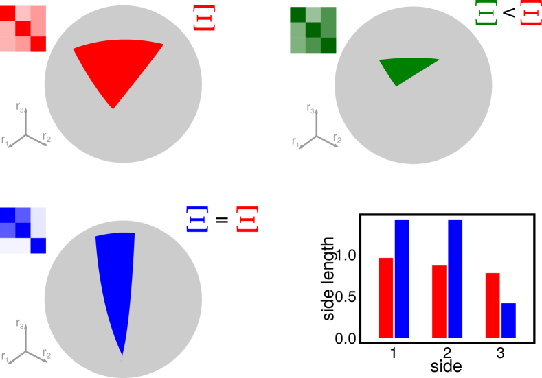
Figure 1: Geometrical properties of feasibility. The panels show the size and shape of the feasibility domain for three interaction matrices, each defining the interactions between three populations. If $\boldsymbol{r}$ corresponds to a feasible equilibrium, so does $c\boldsymbol{r}$ for any positive $c$; one can therefore study the feasibility domain on the surface of a sphere Svirezhev1978 (Supplementary Information). The gray sphere represents the $S=3$-dimensional space of growth rates, while the colored part corresponds to the combination of growth rates leading to stable coexistence. The area (or volume for higher–dimensional systems) of the colored part is measured by $\Xi$. Larger values of $\Xi$ correspond to a higher fraction of growth rate combinations leading to coexistence: the red interaction matrix is therefore more robust against perturbations of $\boldsymbol{r}$ than the green one. The size of this region (i.e., the value of $\Xi$) does not capture all the properties relevant for coexistence. The red and blue systems have the same $\Xi$, but the two regions–despite having the same area–have very different shapes, summarized in the bottom–right panel, where we show the length of each side for the red and blue systems. In the red system, the three sides have about the same length, and thus moving from the center in any direction will have about the same effect. In the blue system however, one side is much shorter than the other two, implying that even small perturbations falling along this direction may drive the system outside the feasibility domain. One of our main results is that, roughly speaking, if the red system corresponds to the random case, then the green one to food webs (having the same heterogeneity in side lengths as the random case but with a smaller $\Xi$ overall), and the blue one to empirical mutualistic networks ($\Xi$ rougly the same as in the random case but with the heterogeneity in side lengths much greater).

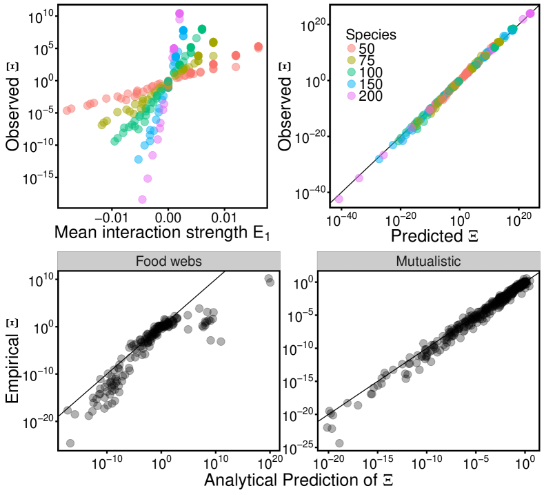
Figure 2: Feasibility domain in random and empirical webs. The top two panels show $\Xi$, the size of the domain of growth rates leading to coexistence, in the case of random networks. The left panel shows the dependence of $\Xi$ on $E_{1}=C\mu$ (where $C$ is the connectance and $\mu$ is the mean interaction strength), and the number of species $S$. The right panel shows the match between our analytical prediction (Eq. 2 and Supplementary Information) and the numerical value of $\Xi$. The bottom panels show a comparison between $\Xi$ computed for empirical webs (89 mutualistic networks on the right, and 15 network was parameterized with different distributions of interaction strengths (Methods). Mutualistic networks have values of $\Xi$ comparable with random networks with similar interactions ($R^{2}=0.98$), indicating that their structure has little effect on the size of the feasibility domain. Food webs have lower values of $\Xi$ than their random counterparts ($R^{2}=0.80$). Empirical networks were parameterized extracting interaction strengths from a bivariate normal distribution with different means, variances, and correlations (Supplementary Information).

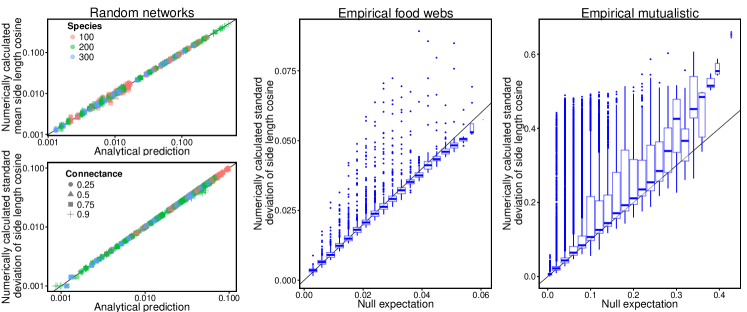
Figure 3: Distribution of side lengths in random, structured, and empirical networks. Left panels show the mean and the standard deviation of $\cos(\eta)$, where $\eta$ is the side length. Analytical predictions for the first two moments of $\cos(\eta)$ (Supplementary Information) perfectly match the numerical simulations. The two panels on the right show the standard deviation of $\cos(\eta)$ for mutualistic and food webs compared to the expectations for the randomized cases. Both trophic and mutualistic interactions show larger fluctuations of side lengths, suggesting the existence of perturbation directions to which the system is more sensitive than to others. This effect is particularly pronounced and relevant for mutualistic networks. While mutualistic and random networks have a similar feasibility domain size $\Xi$, this result implies that the response of mutualistic networks to perturbations is in fact more heterogeneous than those of their random counterparts.

The geometry of coexistence in large ecosystems
Supplementary Information

Contents

1. S1 Community dynamics, feasibility, and stability
2. S2 Disentangling stability and feasibility
3. S3 Geometrical properties of the feasibility domain
4. S4 Definition and calculation of $\Xi$
5. S5 Stability, negative definiteness, and feasibility in random matrices
   1. S5.1 Known results on the spectra of random matrices
   2. S5.2 Universality of $\Xi$
6. S6 Mean-field approximation of $\Xi$
7. S7 Feasibility of consumer-resource communities
8. S8 Empirical networks and randomizations
   1. S8.1 Mutualistic networks
   2. S8.2 Food webs
9. S9 Randomization of empirical networks: assessing the role of structure
   1. S9.1 Mutualistic networks
   2. S9.2 Food webs
10. S10  Possible biases in previous analysis of structural stability
11. S11  Distribution of side lengths
    1. S11.1  The distribution of side lengths in random matrices
    2. S11.2  Moments for random matrices
12. S12  Side heterogeneity for different structures and empirical networks
13. S13  Feasibility domain for $S=3$
14. S14  Nonlinear per capita growth rates

S1 Community dynamics, feasibility, and stability

We consider an ecological community composed of $S$ populations, whose dynamics is described by the following equations:

$$\frac{\mathrm{d}n_{i}}{\mathrm{d}t}=n_{i}\left(r_{i}+\sum_{j=1}^{S}A_{ij}n_{j}\right)\ ,$$ (S1)

where $n_{i}$ is the population abundance of species $i$ and $r_{i}$ is its intrinsic growth rate, and $A_{ij}$ is the effect of a unit change in species $j$’s density on species $i$’s per capita growth rate. For notational convenience, we collect the coefficients $A_{ij}$ into the interaction matrix $\boldsymbol{A}$, and $n_{i}$ and $r_{i}$ into the vectors $\boldsymbol{n}$ and $\boldsymbol{r}$, respectively.

In principle, the interaction matrix $\boldsymbol{A}$ may depend on $\boldsymbol{n}$. We discuss this more general case in section S14. In the following, we consider the simpler case of $\boldsymbol{A}$ being independent of $\boldsymbol{n}$; then, equation (S1) is a general system of Lotka–Volterra population equations.

A vector $\boldsymbol{n}^{\ast}$ is a fixed point (equilibrium) if

$$0=n^{\ast}_{i}\Bigl{(}r_{i}+\sum_{j=1}^{S}A_{ij}n^{\ast}_{j}\Bigr{)}\qquad(i=1,2,\ldots,S)\ .$$ (S2)

A fixed point is feasible if $n^{\ast}_{i}>0$ for all $i$. A feasible fixed point (if it exists) is then a solution to the equation

$$r_{i}=-\sum_{j=1}^{S}A_{ij}n^{\ast}_{j}\ ,$$ (S3)

and therefore, assuming $\boldsymbol{A}$ is invertible,

$$n^{\ast}_{i}=-\sum_{j=1}^{S}(A^{-1})_{ij}r_{j}\ .$$ (S4)

A fixed point $n^{\ast}_{i}$ is locally stable if the system returns to it following any sufficiently small perturbation of the population abundances. Introducing $n_{i}=n^{\ast}_{i}+\delta n_{i}$ in equation S1 and assuming that $\delta n_{i}$ is small, we obtain, by expanding around $\delta n_{i}=0$,

$$\frac{\mathrm{d}\delta n_{i}}{\mathrm{d}t}=\sum_{j=1}^{S}M_{ij}\delta n_{j}\ ,$$ (S5)

where $M_{ij}$ is the $(i,j)$th entry of the Jacobian evaluated at the fixed point (also called the community matrix), which, in the case of equation S1, reduces to

$$M_{ij}=n_{i}^{\ast}A_{ij}=-\left(\sum_{k=1}^{S}(A^{-1})_{ik}r_{k}\right)A_{ij}\ .$$ (S6)

Substituting into equation S5, we get

$$\frac{\mathrm{d}\delta n_{i}}{\mathrm{d}t}=-\sum_{j=1}^{S}\left(\sum_{k=1}^{S}(A^{-1})_{ik}r_{k}\right)A_{ij}\delta n_{j}\ .$$ (S7)

There are two possible scenarios for the dynamics of equation S5. If all eigenvalues of $\boldsymbol{M}$ have negative real parts, then the perturbation $\delta\boldsymbol{n}$ decays exponentially to zero and $n_{i}^{\ast}$ is locally stable. If at least one eigenvalue of $\boldsymbol{M}$ has a positive real part, then there exists an infinitesimal perturbation such that the system does not return to equilibrium. If we order the eigenvalues $\lambda_{i}$ of $\boldsymbol{M}$ according to their real parts, i.e., $\Re(\lambda_{1})>\Re(\lambda_{2})>\dots>\Re(\lambda_{S})$, then stability depends exclusively on $\Re(\lambda_{1})$: if it is negative, $n_{i}^{\ast}$ is dynamically locally stable; otherwise, it is unstable Svirezhev1978 .

A fixed point is globally stable if it is the final outcome of the dynamics from any initial condition involving strictly positive population abundances.

S2 Disentangling stability and feasibility

As we can see from equations S4 and S7, both feasibility and stability depend on both $\boldsymbol{r}$ and $\boldsymbol{A}$ and, at least in principle, a fixed point can be stable or unstable, independently of the fact that it is feasible or not.

We want to study the proportion of conditions (i.e., the number of combinations of the growth rates $\boldsymbol{r}$ out of all possible combinations) leading to coexistence, i.e., leading to stable and feasible equilibria. Therefore in principle we should, for a fixed matrix $\boldsymbol{A}$, look for growth rates $\boldsymbol{r}$ that satisfy both stability and feasibility. In probabilistic terms, we want to measure the likelihood that a random combination of the intrinsic growth rates corresponds to a stable and feasible solution.

In the case of equation S1, it is possible to disentangle feasibility and stability by applying a mild condition on the interaction matrix $\boldsymbol{A}$. To this end, we introduce some terminology (Kaszkurewicz2000, , section 2.1.2):

• Stability. A real matrix $\boldsymbol{B}$ is stable if all its eigenvalues have negative real parts.

• D-stability. A real matrix $\boldsymbol{B}$ is D-stable if $\boldsymbol{D}\,\boldsymbol{B}$ is stable for any diagonal matrix $\boldsymbol{D}$ with strictly positive diagonal entries.

• Diagonal stability. A real matrix $\boldsymbol{B}$ is diagonally stable if there exists a positive diagonal matrix $\boldsymbol{D}$ such that $\boldsymbol{D}\,\boldsymbol{B}+\boldsymbol{B}^{T}\,\boldsymbol{D}$ is stable (where $\boldsymbol{B}^{T}$ is the transpose of $\boldsymbol{B}$).

We also consider

• Negative definiteness (in a generalized sense). A real matrix $\boldsymbol{B}$ is negative definite if $\sum_{ij}x_{i}B_{ij}x_{j}<0$ for any non-zero vector $\boldsymbol{x}$ Johnson1970 .

These properties are closely related to each other berman1983matrix ; Kaszkurewicz2000 :

$$\text{Negative definiteness}\implies\text{Diagonal stability}\implies\text{{D}-stability}\implies\text{Stability}$$ (S8)

• Negative definiteness $\implies$ Diagonal stability. A matrix $\boldsymbol{B}$ is negative definite if and only if all the eigenvalues of $\boldsymbol{B}+\boldsymbol{B}^{T}$ are negative Johnson1970 . If this condition hold, then the positive diagonal matrix satisfying the definition of diagonal stability is simply the identity matrix.

• Diagonal stability $\implies$ D-stability. See the book by Kaszkurewicz & Bhaya for the proof (Kaszkurewicz2000, , lemma 2.1.4).

• D-stability $\implies$ Stability. This follows from the definition of D-stability when $\boldsymbol{D}$ is the identity matrix.

In the case of equation S1, those conditions applied to the matrix $\boldsymbol{A}$ are related to the stability of the system. One can use the definition of the community matrix (equation S6) to show that D-stability of $\boldsymbol{A}$ implies the local asymptotic stability of any feasible fixed point. This is because the community matrix with entries $M_{ij}=n_{i}^{\ast}A_{ij}$ can be written as $\boldsymbol{N}\,\boldsymbol{A}$, where $\boldsymbol{N}$ is the diagonal matrix with $N_{ii}=n^{\ast}_{i}$. If the fixed point is feasible and $\boldsymbol{A}$ is D-stable, then local asymptotic stability is guaranteed. Moreover it is possible to show Goh1977 ; Rohr2014 that diagonal stability of $\boldsymbol{A}$ $\implies$ global stability.

Thus, we have a condition on $\boldsymbol{A}$ that makes it possible to disentangle the problems of stability and feasibility: $\boldsymbol{A}$ is negative definite $\implies$ global stability of the feasible fixed point Volterra1931 . Therefore, if we assume $\boldsymbol{A}$ is negative definite, then feasibility of the equilibrium is sufficient to guarantee its global stability as well, i.e., feasibility guarantees globally stable coexistence. Consistently with this, it is known that the largest eigenvalue of $(\boldsymbol{A}+\boldsymbol{A}^{T})/2$ is always larger than or equal to the real part of $\boldsymbol{A}$’s leading eigenvalue Tang2014 , i.e. negative definiteness implies stability. While this was indeed observed before, it is important to underline that, in the case of ref. Tang2014 , this property was considered on the community matrix $\boldsymbol{M}$ (which also depends on the fixed point’s position in phase space) and not on the interaction matrix $\boldsymbol{A}$.

Since we are interested in studying how interactions (i.e., the matrix $\boldsymbol{A}$) determine coexistence, and which properties of the former determine the latter, we will restrict our analysis to negative definite matrices $\boldsymbol{A}$ and focus only on the problem of feasibility. This condition has the advantage of being analytically computable for large random matrices (see section S5.1).

S3 Geometrical properties of the feasibility domain

In section S2 we showed how to separate feasibility and stability, i.e., we have a sufficient condition on the interaction matrix that guarantees (global) stability of the feasible fixed point. The problem of determining the size of the coexistence domain is therefore reduced to that of determining the size of the feasibility domain. The ecological interpretation of this volume is the proportion of different conditions leading to feasible equilibria out of all possible conditions. The larger this volume is, the higher the probability that the system is able to sustain biodiversity. In terms of equation S1, we want to quantify the proportion of growth rate vectors $\boldsymbol{r}$ corresponding to a feasible fixed point.

This geometrical approach was pioneered in Svirezhev1978 where the space of feasible solution was studied for dissipative systems, and the size of that domain was computed in the case $S=3$ (see section S13).

At this point, it is important to observe that if a vector $\boldsymbol{r}$ corresponds to a feasible solution, then $c\boldsymbol{r}$, $c$ being an arbitrary positive constant, also corresponds to a feasible solution. This is because the equilibrium solution $n_{i}^{\ast}$ is given by equation S4, which is linear in $r_{i}$. Therefore, the equilibrium corresponding to $cr_{i}$ is simply $cn_{i}^{\ast}$, and since $c$ is positive, $cn_{i}^{\ast}$ is also feasible.

This fact implies that, given a large number of growth rate vectors $\boldsymbol{r}$, the expected proportion of vectors corresponding to a feasible fixed point is independent of $\boldsymbol{r}$’s norm. In other words, $\boldsymbol{r}$ is feasible if and only if $\boldsymbol{r}/\|\boldsymbol{r}\|$ is feasible, where $\|\boldsymbol{r}\|=\sqrt{\sum_{i}r_{i}^{2}}$ is the Euclidean norm of $\boldsymbol{r}$. The proportion of feasible growth rates among all possible ones is therefore equal to the proportion of feasible growth rates calculated using only growth rate vectors with $\|\boldsymbol{r}\|=1$; i.e., those lying on the unit sphere.

Before proceeding with the mathematical definition of the size of the feasibility domain, we discuss the geometrical interpretation of equation S4. From this equation, the feasibility condition reads

$$\sum_{j=1}^{S}(A^{-1})_{ij}r_{j}<0\ .$$ (S9)

This equation defines a convex polyhedral cone in the $S$-dimensional space of growth rates. A convex polyhedral cone Rockafellar1997 is a subset of $\mathbb{R}^{S}$ whose elements $\boldsymbol{x}$ can be written as positive linear combinations of $N_{G}$ different $S$-dimensional vectors $\boldsymbol{g}^{k}$ called the generators of the cone:

$$\boldsymbol{x}=\sum_{k=1}^{N_{G}}\boldsymbol{g}^{k}\lambda_{k}\ ,$$ (S10)

where the $\lambda_{k}$ are arbitrary positive constants. Due to this arbitrariness, if $\boldsymbol{g}^{k}$ is a generator of a given convex polyhedral cone, then also $c\boldsymbol{g}^{k}$ (where we rescale just the $k$th generator with the positive constant $c$, leaving the others unchanged) will be a generator of the same cone Svirezhev1978 . In the case of equation S3, each and every growth rate vector belonging to the feasibility domain can be written as

$$r_{i}=-\sum_{k=1}^{S}A_{ik}n^{\ast}_{k}\ ,$$ (S11)

where, by definition, $n^{\ast}_{k}$ is feasible and therefore a positive constant. One can easily see that this equation corresponds to equation S10 where the number of generators $N_{G}$ is equal to $S$ and the $i$th component of the vector $\boldsymbol{g}^{k}$ is proportional to $-A_{ik}$. As the lengths of the generators can be set to any positive value, we will normalize them to one, i.e.,

$$g^{k}_{i}(\boldsymbol{A})=\frac{-A_{ik}}{\sqrt{\sum_{j=1}^{S}(A_{jk})^{2}}}\ .$$ (S12)

The generators completely define the feasibility domain in the space of growth rates. A growth rate vector corresponds to a feasible equilibrium if and only if it can be written as a linear combination of the generators with positive coefficients. Biologically the generators correspond to the growth rate vectors that bound the coexistence domain. They correspond to nonfeasible equilibria with just one species with positive abundance (and all the others with zero abundance), such that there exist arbitrarily small perturbations of the growth rate vector that make the equilibrium feasible.

The set of all the growth rate vectors leading to a feasible equilibrium is therefore a convex polyhedral cone, defined by

$$K(\boldsymbol{A})=\{\boldsymbol{r}\in\mathbb{R}^{S}|\sum_{j=1}^{S}(A^{-1})_{ij}r_{j}<0\}\ .$$ (S13)

Equivalently, it can be defined in terms of the generators:

$$K(\boldsymbol{A})=\{\boldsymbol{r}\in\mathbb{R}^{S}|\exists\lambda_{1},\lambda_{2},\dots,\lambda_{k}>0,\boldsymbol{r}=\sum_{k=1}^{S}\boldsymbol{g}^{k}(\boldsymbol{A})\lambda_{k}\}\ ,$$ (S14)

where the generators $\boldsymbol{g}^{k}(\boldsymbol{A})$ are defined in equation S12. In section S13 we show explicitly how these concepts pan out in the case of $S=3$.

This geometrical definition and characterization of the feasibility domain allows us to identify classes of matrices having the exact same feasibility domain: they are simply matrices having the same set of generators. In particular, there are two basic transformations of the matrix $\boldsymbol{A}$ (and their combinations) that leave the set of generators unchanged: permutations and positive rescaling. A square matrix $\boldsymbol{P}$ is a permutation matrix if each row and column has one and only one nonzero entry and the value of that entry is equal to one. A positive rescaling is performed by a positive diagonal matrix $\boldsymbol{D}$. The set of generators of $\boldsymbol{A}$ is the same as those of $\boldsymbol{P}\,\boldsymbol{A}$ and $\boldsymbol{D}\,\boldsymbol{A}$. This can be seen by observing that a permutation of the rows just changes the order of the generators but not the generators themselves. In the same way, a generator with the same direction but different length generates the same cone, and so any positive constant that rescales a row of the matrix leaves the feasibility domain unchanged. It is important to note however that these two transformations do not leave the properties of the matrix $\boldsymbol{A}$ unchanged: both exchanging rows of a matrix and rescaling rows by different constants will in general change the structure of the matrix.

Using this geometrical framework, one can easily identify the center of the feasibility domain (also known as structural vector Rohr2014 ). There are several possible ways to define the center of a hypervolume and, without additional assumptions, all the definitions are different. One natural choice is the barycenter (“center of mass”) of the domain of feasible intrinsic growth rates. Any plane passing through the barycenter divides the volume into two subvolumes of equal size. The barycenter is equivalent to the center of mass of the volume (in the case of constant density). Then, the vector $\boldsymbol{x}^{b}$ pointing from the origin to the barycenter is given by

$$\boldsymbol{x}^{b}=\int_{K(A)\cap\mathbb{S}_{S}}\mathrm{d}^{S}\boldsymbol{y}\ \ \boldsymbol{y}\ ,$$ (S15)

where $\cap$ is the intersection of two sets, and $\mathbb{S}_{S}=\{\boldsymbol{r}\in\mathbb{R}^{S}|\|\boldsymbol{r}\|=1\}$ represents the surface of the $S$-dimensional unit sphere. The variable $\boldsymbol{y}$ is therefore integrated over the feasibility domain restricted to the unit sphere’s surface. All points in the feasibility domain are positive linear combinations of the generators, i.e.,

$$\boldsymbol{y}=\sum_{k}\lambda^{k}\boldsymbol{g}^{k}\ \ ,$$ (S16)

where the $\lambda^{k}$ are positive constants. The fact that we consider only the points lying on the unit sphere, i.e., $\|\boldsymbol{y}\|=1$, can be expressed as a constraint on $\boldsymbol{\lambda}$ (the vector of $\lambda$s). Thus, we can write equation S15 as

$$\boldsymbol{x}^{b}=\int\mathrm{d}^{S}\boldsymbol{\lambda}\,q(\boldsymbol{\lambda})\sum_{k}\lambda^{k}\boldsymbol{g}^{k}\ ,$$ (S17)

where $q$ is an appropriate distribution, introduced to take into account three different constraints: all the components of $\boldsymbol{\lambda}$ must be positive; the vector $\sum_{k}\lambda^{k}\boldsymbol{g}^{k}$ must lie on the unit sphere; and those vectors must be sampled uniformly on the feasibility domain. One can show that the distribution $q(\boldsymbol{\lambda})$ has the following form

$$q(\boldsymbol{\lambda})\propto\exp\left(-\sum_{i,j}\lambda^{i}(\boldsymbol{g}^{i}\cdot\boldsymbol{g}^{j})\lambda^{j}\right)\prod_{k}\Theta(\lambda^{k})\ ,$$ (S18)

where the proportionality constant is given by the normalization. Therefore, by defining,

$$\int\mathrm{d}^{S}\boldsymbol{\lambda}\,q(\boldsymbol{\lambda})\ \lambda^{k}=:\langle\lambda^{k}\rangle\ ,$$ (S19)

we obtain

$$\boldsymbol{x}^{b}=\sum_{k}\boldsymbol{g}^{k}\int\mathrm{d}^{S}\boldsymbol{\lambda}\,q(\boldsymbol{\lambda})\ \lambda^{k}=\sum_{k}\boldsymbol{g}^{k}\langle\lambda^{k}\rangle\ .$$ (S20)

S4 Definition and calculation of $\Xi$

As explained in section S3, the proportion of feasible growth rates can be calculated considering only growth rate vectors of length one, i.e., $\|\boldsymbol{r}\|=1$. This proportion can be interpreted as the volume of the intersection of a convex cone and the surface of a sphere. Equivalently, it is the solid angle of the convex polyhedral cone Ribando2006 ; Gourion2010 .

We define the quantity $\Xi$ as

$$\Xi=2^{S}\,\frac{\text{\# growth rate vectors corresponding to a feasible fixed point}}{\text{total \# growth rate vectors}}\ .$$ (S21)

The factor $2^{S}$ that appears in this equation is an arbitrary choice, and it has been introduced to have $\Xi=1$ when species are not interacting ($A_{ij}=0$ if $i\neq j$). In this case equation S1 reduces to $S$ independent logistic equations with equilibrium densities $n_{i}^{\ast}=-r_{i}/A_{ii}$. Taking each $A_{ii}$ to be negative (otherwise each species would have an unstoppable positive feedback on itself), this equilibrium is feasible if and only if each $r_{i}$ is positive. For a single species then, the probability of randomly drawing a feasible (i.e., positive) growth rate out of all possible growth rates is one half. For two species, both growth rates must have the correct sign to have the two species with positive abundance, and therefore the proportion of growth rate vectors satisfying this condition is $1/4$. For $S$ species the combinations of the growth rates leading to a feasible fixed point is $2^{-S}$. $\Xi$, defined as in equation S21, is therefore equal to one when species do not interact.

In terms of geometrical properties and the convex polyhedral cone, $\Xi$ can be defined as

$$\Xi=2^{S}\frac{\operatorname*{\mathrm{vol}}_{S-1}(K(A)\cap\mathbb{S}_{S})}{\operatorname*{\mathrm{vol}}_{S-1}(\mathbb{S}_{S})}\ ,$$ (S22)

where $K(A)$ is defined in equation S13, $\mathbb{S}_{S}$ is the unit sphere in $\mathbb{R}^{S}$, while $\operatorname*{\mathrm{vol}}_{S}(\cdot)$ means volume in $S$ dimensions. This definition is equivalent to the one in equation S21Ribando2006 ; Gourion2010 .

These two equivalent definitions can be expressed in terms of an integral in the space of the growth rate vectors:

$$\Xi=\frac{2^{S}}{\operatorname*{\mathrm{vol}}_{S-1}(\mathbb{S}_{S})}\int_{\mathbb{R}^{S}}\mathrm{d}^{S}\boldsymbol{r}\ 2\|\boldsymbol{r}\|\,\delta(\|\boldsymbol{r}\|^{2}-1)\ \prod_{i=1}^{S}\Theta(n_{i}^{\ast}(\boldsymbol{r}))\ ,$$ (S23)

where $\operatorname*{\mathrm{vol}}_{S-1}(\mathbb{S}_{S})$ is the volume of the unit sphere’s surface in $S$ dimensions, $\Theta(\cdot)$ is the Heaviside function (equal to $1$ is the argument is positive and to zero otherwise), and $\delta(\cdot)$ is the Dirac delta function. In this expression, we integrate over the surface of the $S$-dimensional unit sphere. The integral of a function $f(\boldsymbol{x})$ on the unit sphere is given by

$$\int_{\mathbb{S}_{S}}\mathrm{d}^{S}\boldsymbol{x}\ f(\boldsymbol{x})=\int_{\mathbb{R}^{S}}\mathrm{d}^{S}\boldsymbol{x}\ 2\|\boldsymbol{x}\|\delta(\|\boldsymbol{x}\|^{2}-1)\ f(\boldsymbol{x})\ ,$$ (S24)

where the term $\delta(\|\boldsymbol{x}\|^{2}-1)$ that appears in the integration constrains $\boldsymbol{x}$ on the surface of the unit sphere, and the factor $2\|\boldsymbol{x}\|$ is the derivative of the delta function’s argument, which is needed because the Dirac delta is nonlinear in $\|\boldsymbol{r}\|$. The factor $\operatorname*{\mathrm{vol}}_{S-1}(\mathbb{S}_{S})$, the surface of sphere in $S$ dimensions, can be obtained by setting $f(x)=1$:

$$\mathrm{vol}_{S-1}(\mathbb{S}_{S})=\int\mathrm{d}^{S}\boldsymbol{x}\ 2\|\boldsymbol{x}\|\delta(\|\boldsymbol{x}\|^{2}-1)=\frac{2\pi^{S/2}}{\Gamma(S/2)}\ ,$$ (S25)

where $\Gamma(\cdot)$ is the Gamma function. Finally, the term $\prod_{i=1}^{S}\Theta(\boldsymbol{n}_{i}^{\ast}(\boldsymbol{r}))$ in equation S23 expresses the constraint of all $n_{i}^{\ast}$ having to be positive: this product is equal to $1$ if the equilibrium $\boldsymbol{n}^{\ast}(\boldsymbol{r})$ is feasible and zero otherwise. The equilibrium $\boldsymbol{n}^{\ast}(\boldsymbol{r})$ is a function of $\boldsymbol{r}$ via equation S4.

Equation S23 defines $\Xi$ as the volume of the domain of growth rates leading to feasible solutions. Using the results of section S2, we know that if the interaction matrix $\boldsymbol{A}$ is negative definite then a feasible fixed point is globally stable. In this case $\Xi$ is the volume of the domain of intrinsic growth rates leading to feasible and (globally) stable solutions.

Unfortunately, direct numerical computation of $\Xi$ is inefficient when the number of species $S$ is large. To evaluate the integral in equation S23, e.g., via Monte Carlo integration, we should draw intrinsic growth rates at random and count how many of them, out of the total, lead to a feasible equilibrium. In order to have a reliable estimate of this proportion, we should sample the space in such a way that the number of feasible growth rates found is large. This goal requires an exponentially increasing sampling effort as $S$ increases. In this section we provide an alternative, much faster and reliable, way of estimating $\Xi$.

The equilibrium solution and the growth rates are linearly related via $r_{i}=-\sum_{i=1}^{S}A_{ij}n_{j}^{\ast}$ (equation S3). Our strategy is to use this to perform a change of variables in equation S23, and integrate over $\boldsymbol{n}^{\ast}$ instead of $\boldsymbol{r}$. Since $\boldsymbol{A}$ is negative definite (and thus stable and not singular), it is invertible, and so it is always possible to perform this change of variables. Note that, more generally, the change of variables can be performed if $A$ is nonsingular (i.e., $\det(A)=0$). We then obtain

$$\Xi=\frac{2^{S}\ \Gamma(S/2)\ |\det(\boldsymbol{A})|}{2\pi^{S/2}}\int_{\mathbb{R}^{S}}\mathrm{d}^{S}\boldsymbol{n}^{\ast}\ 2\delta\left(\sum_{i,j,k}n_{i}^{\ast}A_{ki}A_{kj}n_{j}^{\ast}-1\right)\ \prod_{i=1}^{S}\Theta(n_{i}^{\ast})\ ,$$ (S26)

where $|\det(\boldsymbol{A})|$ is the determinant of $\boldsymbol{A}$, which is also the Jacobian of the change of variables. After the change of variables, the integration is now performed over the feasible equilibrium points and so the condition of feasibility is automatically implemented.

It is still difficult to evaluate the previous expression numerically, because of the constraint that appears in the delta function. We can further simplify it by introducing polar coordinates. In particular, we write the vector $\boldsymbol{n}$ as $\boldsymbol{n}=n\boldsymbol{u}$, where $n=\|\boldsymbol{n}\|$ and $\boldsymbol{u}$ is a vector of unit length. We can perform a new change of variables, passing from $\boldsymbol{n}$ to $n$ and $\boldsymbol{u}$. Specifically, for any function $f(\boldsymbol{n})$, we can write

$$\int_{\mathbb{R}^{S}}\mathrm{d}^{S}\boldsymbol{n}\ f(\boldsymbol{n})=\int_{0}^{\infty}\mathrm{d}n\ n^{S-1}\ \int_{\mathbb{R}^{S}}\mathrm{d}^{S}\boldsymbol{u}\ 2\delta(\|\boldsymbol{u}\|^{2}-1)f(n\boldsymbol{u})=\int_{0}^{\infty}\mathrm{d}n\ n^{S-1}\ \int_{\mathbb{S}_{S}}\mathrm{d}^{S}\boldsymbol{u}\ f(n\boldsymbol{u})\ .$$ (S27)

Using this expression in equation S26, we obtain

$$\Xi=\frac{2^{S}\ \Gamma(S/2)\ \det(\boldsymbol{A})}{2\pi^{S/2}}\int_{0}^{\infty}\mathrm{d}n\ n^{S-1}\ \int_{\mathbb{S}_{S}}\mathrm{d}^{S}\boldsymbol{u}\ 2\delta\left(n^{2}\sum_{i,j}u_{i}G_{ij}u_{j}-1\right)\ \prod_{i=1}^{S}\Theta(u_{i})\ ,$$ (S28)

where we used the fact that $\Theta(n_{i})=\Theta(u_{i})$ (since $n_{i}=nu_{i}$, and $n$ is positive by definition), and we have introduced the matrix $G_{ij}=\sum_{k}A_{ki}A_{kj}$. We can now perform the integration over $n$, obtaining

$$\begin{split}\displaystyle\int_{0}^{\infty}\mathrm{d}n&\ n^{S-1}\ 2\ \delta\left(n^{2}\sum_{i,j}u_{i}G_{ij}u_{j}-1\right)\\ =&\int_{0}^{\infty}\mathrm{d}n\ n^{S-1}\ 2\ \delta\left(n-\frac{1}{\sqrt{\sum_{i,j}u_{i}G_{ij}u_{j}}}\right)\ \frac{1}{2n\sum_{i,j}u_{i}G_{ij}u_{j}}=\displaystyle\left(\sum_{i,j}u_{i}G_{ij}u_{j}\right)^{-S/2}\ ,\end{split}$$ (S29)

and therefore the integral of equation S23 finally reads

$$\Xi=\frac{2^{S}\ \Gamma(S/2)\ \sqrt{\det(\boldsymbol{G})}}{2\pi^{S/2}}\int_{\mathbb{S}_{S}}\mathrm{d}^{S}\boldsymbol{u}\ \prod_{i=1}^{S}\Theta(u_{i})\ \left(\sum_{i,j}u_{i}G_{ij}u_{j}\right)^{-S/2}\ ,$$ (S30)

where we have used the fact that $\det(\boldsymbol{G})=\det(\boldsymbol{A}^{T}\boldsymbol{A})=\det(\boldsymbol{A})^{2}$. In terms of the interaction matrix, the equation reads

$$\Xi=\frac{2^{S}\ \Gamma(S/2)\ |\det(\boldsymbol{A})|}{2\pi^{S/2}}\int_{\mathbb{S}_{S}}\mathrm{d}^{S}\boldsymbol{u}\ \prod_{i=1}^{S}\Theta(u_{i})\ \left(\sum_{i,j,k}u_{i}A_{ki}A_{kj}u_{j}\right)^{-S/2}\ .$$ (S31)

Equation S30 shows explicitly the role of the generators. The matrix $\boldsymbol{G}$ can indeed be rewritten as

$$G_{ik}=\sum_{j}g^{i}_{j}g^{k}_{j}c_{i}c_{k}=c_{i}c_{k}\boldsymbol{g}^{i}\cdot\boldsymbol{g}^{k}\ ,$$ (S32)

where $g^{k}_{j}$ are the generators of the convex cone defined in equation S12 and $c_{i}$ are arbitrary positive constants. Their presence, which can be seen as a change of the normalization of the vectors $\boldsymbol{g}^{k}$, does not affect the form of equation S30 and its dependence on $\boldsymbol{G}$ (see section S3). This property can be checked explicitly from equation S30, by introducing an explicit dependence on $c_{i}$ and showing that $\Xi$ is independent of their values.

Unfortunately, the integral in equation S30 cannot be computed analytically. As mentioned before, when the integral is written in the form of equation S23 it is impractical to evaluate it numerically, since it would require an exponentially increasing sampling to get a reasonable precision. Fortunately, this is not the case when the integral is written as in equations S30 and S31. The main difference is that, after changing variables, we are directly sampling the space of feasible solutions, without losing computational time in randomly exploring the space of intrinsic growth rates looking for feasible solutions.

To evaluate the integral, we use the usual approach of Monte Carlo algorithms. In particular, it is possible to write the integral as an average over random points:

$$\frac{1}{T}\sum_{a=1}^{T}\Bigl{(}\sum_{i,j}u^{a}_{i}G_{ij}u^{a}_{j}\Bigr{)}^{-S/2}\to\frac{\Gamma(S/2)}{2\pi^{S/2}}\int d^{S}u\ \prod_{i=1}^{S}\Theta(u_{i})\ 2\delta(\|u\|^{2}-1)\ \Bigl{(}\sum_{i,j}u_{i}G_{ij}u_{j}\Bigr{)}^{-S/2}$$ (S33)

when $T\to\infty$. In this expression $\boldsymbol{u}^{a}$ are independently drawn random vectors uniformly distributed on the unit sphere and with only positive components. These two conditions are introduced to satisfy the constraints $\prod_{i=1}^{S}\Theta(u_{i})$ and $2\delta(\|u\|^{2}-1)$ that appear in the integral. $T$ is the sample size, and the average on the left hand side of equation S33 converges to the right hand side in the large $T$ limit.

One always has a finite sample size $T$, used to approximate the integral. It is therefore important to have an estimate of the error made due to $T<\infty$. Since the left hand side of equation S33 is an average of a function over random vectors, this error can be estimated by simply using the variance of the function’s values. In particular, the error $\sigma_{\text{MC}}$ is defined as

$$\sigma_{\text{MC}}=\frac{1}{\sqrt{T}}\sqrt{\frac{1}{T}\sum_{a=1}^{T}\left(\sum_{i,j}u^{a}_{i}G_{ij}u^{a}_{j}\right)^{-S}-\left(\frac{1}{T}\sum_{a=1}^{T}\left(\sum_{i,j}u^{a}_{i}G_{ij}u^{a}_{j}\right)^{-S/2}\right)^{2}}\ .$$ (S34)

The numerical simulation presented in the work where obtained were obtained with different sampling effort $T$. Instead of fixing $T$ a priori, we determined a precision goal, that we measured in terms of the relative error $\sigma_{MC}/\Xi$. We ran the simulations until $\sigma_{MC}/\Xi<0.05$. In order to avoid artificially small samples and to have enough statistical power not to undershoot to much $\sigma_{\text{MC}}$, we ran $10\times S$ Monte Carlo steps before checking the condition for the first time.

S5 Stability, negative definiteness, and feasibility in random matrices

Random matrices are a useful tool in ecology, and have been studied since May’s seminal paper May1972 . Mostly, they have been used to model the community matrix May1972 ; Allesina2012 . In the context of this work, we use random matrices to model interaction matrices $\boldsymbol{A}$. We consider random matrices constructed in the following way:

• $A_{ii}=-d$ where $d$ is a positive constant.

• Each pair $(A_{ij},A_{ji})$ is set equal to a pair of random variables drawn from a joint distribution with probability density function $q(x,y)$.

• The random variables are exchangeable—i.e., the probability distribution function is symmetric in its arguments: $q(x,y)=q(y,x)$—and all the moments are finite.

We show that the three most important quantities for our problem are the moments

$$E_{1}=\int\mathrm{d}x\ \mathrm{d}y\ xq(x,y)=\int\mathrm{d}x\ \mathrm{d}y\ yq(x,y)\ ,$$ (S35)

$$E_{2}=\sqrt{\int\mathrm{d}x\ \mathrm{d}y\ (x-E_{1})^{2}q(x,y)}=\sqrt{\int\mathrm{d}x\ \mathrm{d}y\ (y-E_{1})^{2}q(x,y)}\ ,$$ (S36)

$$E_{c}=\frac{1}{E_{2}^{2}}\int\mathrm{d}x\ \mathrm{d}y\ (x-E_{1})(y-E_{1})q(x,y)\ .$$ (S37)

In the limit of large $S$, they can be computed as proper sample means of $\boldsymbol{A}$’s entries:

$$E_{1}=\frac{1}{S(S-1)}\sum_{i=1}^{S}\sum_{j\neq i}A_{ij}\ ,$$ (S38)

$$E_{2}=\sqrt{\frac{1}{S(S-1)}\sum_{i=1}^{S}\sum_{j\neq i}(A_{ij})^{2}-E_{1}^{2}}\ ,$$ (S39)

$$E_{c}=\frac{1}{E_{2}^{2}}\left(\frac{1}{S(S-1)}\sum_{i=1}^{S}\sum_{j\neq i}A_{ij}A_{ji}-E_{1}^{2}\right)\ .$$ (S40)

The parameterization used by May May1972 would correspond to

$$q_{\text{May}}(x,y)=\Bigl{(}(1-C)\delta(x)+Cp(x)\Bigr{)}\Bigl{(}(1-C)\delta(y)+Cp(y)\Bigr{)}\ ,$$ (S41)

where $\delta(\cdot)$ is the Dirac delta function and $p(x)$ is an arbitrary distribution with mean zero and variance $\sigma^{2}$. The connectance $C$ sets the probability that each entry is equal to zero (with probability $1-C$) or randomly drawn from the probability distribution $p(x)$ with probability $C$. In this case $E_{1}=E_{c}=0$, while $E_{2}^{2}=C\sigma^{2}$.

In the following, we summarize known results on the spectra, negative definiteness conditions, and properties of $\Xi$ for these matrices.

S5.1 Known results on the spectra of random matrices

Under the assumptions of the previous section, the eigenvalues of $\boldsymbol{A}$ in the limit of large $S$ are uniformly distributed in an ellipse in the complex plane. If $E_{1}\neq 0$ there is always an eigenvalue $\lambda_{m}$ whose value is approximately

$$\lambda_{m}\approx-d+SE_{1}\ ,$$ (S42)

independently of the rest of the eigenvalue distribution. The ellipse is centered at $-d-E_{1}$, its axes are aligned with the real and imaginary axes, and their lengths are

$$a=\sqrt{S}E_{2}(1+E_{c})$$ (S43)

and

$$b=\sqrt{S}E_{2}(1-E_{c})\ .$$ (S44)

If $\lambda_{m}=0$, the eigenvalue with the largest real part(s) is approximated by the rightmost point of the ellipse. The system is stable if its real part is negative. In the most general case, this condition is equivalent to

$$-d+\max\left\{SE_{1},-E_{1}+\sqrt{S}E_{2}(1+E_{c})\right\}<0\ .$$ (S45)

In section S2 we introduced the concept of negative definiteness. In particular, we showed that when the matrix is negative definite then it is possible to disentangle stability and feasibility. The matrix is negative definite if the eigenvalues of $\boldsymbol{A}+\boldsymbol{A}^{T}$ are all negative. This condition reads Tang2014

$$-d+\max\left\{SE_{1},-E_{1}+\sqrt{2S(1+E_{c})}E_{2}\right\}<0\ .$$ (S46)

Figure S1 shows the values of parameters leading to the possible combinations of stability and negative definiteness in random matrices for the case $E_{1}=0$. Since we imposed that $\boldsymbol{A}$ is negative definite, the region of parameters we explore is the one above the negative definiteness line. One can see that in this way we are missing some parameterizations, corresponding to those that lead to a stable but not negative definite matrices. From equations S45 and S46 one can see that the case $E_{1}<0$ is very similar to the case $E_{1}=0$. More interestingly, for $E_{1}>0$, the conditions for stability and negative definiteness converge in the large $S$ limit, implying that we are considering all the possible cases.

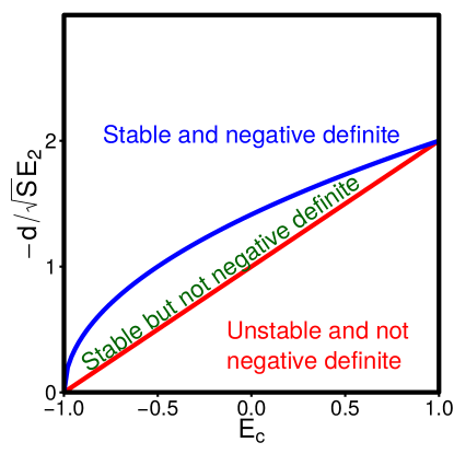
Supplementary Figure S1: Negative definiteness and stability for random matrices in the case $E_{1}=0$. The red curve describes the condition for stability (equation S45), while the blue curve corresponds to the negative definiteness condition (equation S46). The region above the blue curve corresponds to matrices that are both stable and negative definite, while the region below the red curve corresponds to unstable and non-negative definite matrices. The parameterizations that may still lead to stable and feasible points but we are not considering are in the region between the two curves. The shape of this region does not change substantially if $S$ and $E_{2}$ are changed or if $E_{1}<0$. For $E_{1}>0$ the not negative definite but stable region is always smaller and eventually disappears (i.e., the blue and the red curve become the same) when $S$ is large enough.

What is remarkable in these conditions and in the distribution of eigenvalues is that they are universal Tao2010 ; Tao2010a ; Tao2011 ; Allesina2015 . Universality means that they depend only on $S$, $E_{1}$, $E_{2}$, and $E_{c}$ (and $d$, but via a trivial dependence). The spectrum of eigenvalues does not depend on the detailed form of the distribution $q(x,y)$.

For instance, consider the case $q(x,y)=p(x)p(y)$, where the upper and lower triangular entries $A_{ij}$ and $A_{ji}$ are independent random variables. In this case $E_{c}=0$ and $E_{1}$ and $E_{2}$ are the mean and standard deviation of the distribution $p(x)$. The distribution of eigenvalues and the conditions for stability and negative definiteness are the same for any probability distribution $p(x)$ as long as their mean $E_{1}$ and standard deviation $E_{2}$ are the same (provided some mild conditions on higher moments hold). For instance, a Lognormal distribution, a Gaussian distribution and an exponential distribution, having same mean and standard deviation, produce the same eigenvalue distribution, and therefore the same conditions for stability ReviewRMT .

From an ecological perspective, one can consider different interaction matrices corresponding to different interaction types. The interaction type is given by the signs of the pairs $(A_{ij},A_{ji})$: competitive interactions will have both entries with a negative sign, while in trophic interactions the entries will have opposite sign. The interaction pairs $(A_{ij},A_{ji})$ for competitive interactions can for instance be obtained from the following distribution:

$$q_{\text{comp}}(x,y)=(1-C)\delta(x)\delta(y)+Ch_{-}(x)h_{-}(y)\ ,$$ (S47)

where $h_{-}$ is a probability distribution function with support on the negative axis (i.e., the random variables are always negative), and $C$ is the connectance (a pair is different from zero with probability $C$). In the case of trophic interactions we could consider

$$q_{\text{troph}}(x,y)=(1-C)\delta(x)\delta(y)+\frac{C}{2}p_{-}(x)p_{+}(y)+\frac{C}{2}p_{+}(x)p_{-}(y)\ ,$$ (S48)

where $p_{+}$ and $p_{-}$ are two probability distribution functions with positive and negative support, respectively. Suppose that the moments of $h_{-}$, $p_{+}$, and $p_{-}$ are chosen in such a way that $q_{\text{comp}}(x,y)$ and $q_{\text{troph}}(x,y)$ have the same values of $E_{1}$, $E_{2}$, and $E_{c}$. The interaction matrices will still look very different in the two cases: one describes a foodweb and the other a competitive system. Despite this difference, the two will have the same stability properties. In other words, different interaction types influence the stability properties of the system only via $E_{1}$, $E_{2}$ and $E_{c}$.

S5.2 Universality of $\Xi$

In this section we show that, apart from their spectral distribution, $\Xi$ is also a universal quantity in large random matrices. That is, in the large $S$ limit, its value does not depend on the entire distribution of the coefficients, but only on the three moments $E_{1}$, $E_{2}$, and $E_{c}$. It is important to remark that this result applies to the large $S$ limit: the sub-leading corrections depend in principle on all the moments.

In order to show that $\Xi$ is universal, we parameterized random networks with different distributions and checked whether $\Xi$ depends only on $E_{1}$, $E_{2}$, $E_{c}$, and $S$, but not on other properties. To do this, we constructed several $S\times S$ matrices. Each individual matrix had its entries drawn from some fixed distribution, but the shape of the distribution was different across matrices. However, regardless of the distribution’s shape, their moments were fixed at $E_{1}$, $E_{2}$, and $E_{c}$. We then checked whether these matrices led to the same value of $\Xi$.

In our simulations we considered a distribution of the pairs $(A_{ij},A_{ji})$ of the form

$$q(x,y)=(1-C)\delta(x)\delta(y)+Cp(x,y)\ ,$$ (S49)

where the connectance $C$ is the probability that two species $i$ and $j$ interact. The probability distribution $p(x,y)$ in equation S49 depends on three parameters $\mu$, $\sigma$, and $\rho$, which define the mean, variance, and correlation of the pairs drawn from $p(x,y)$. Given the values of $E_{1}$, $E_{2}$, and $E_{c}$, we can arbitrary choose $C$ and tune $\mu$, $\sigma$, and $\rho$ to obtain any desired $E_{1}$, $E_{2}$, and $E_{c}$. If $\Xi$ is universal, then different matrices built with different values of $C$, $\mu$, $\sigma$, and $\rho$ but the same values of $E_{1}$, $E_{2}$, and $E_{c}$ will lead to the same $\Xi$.

We considered five parameterizations of the distribution $p(x,y)$:

• Random signs, normal distribution:

  $$p(x,y)=BN(x,y|\mu,\sigma,\rho)\ .$$ (S50)

  The distribution $BN(x,y|\mu,\sigma,\rho)$ is a bivariate normal distribution with marginal means equal to $\mu$, marginal variances equal to $\sigma^{2}$, and correlation equal to $\rho\sigma^{2}$. The pairs can in principle assume all possible combinations of signs.

• Random signs, four corners:

  $$\begin{split}p(x,y)=&\frac{q}{2}\delta(x-\mu-\sigma)\delta(y-\mu-\sigma)+\frac{q}{2}\delta(x-\mu+\sigma)\delta(y-\mu+\sigma)\\ +&\frac{1-q}{2}\delta(x-\mu-\sigma)\delta(y-\mu+\sigma)+\frac{1-q}{2}\delta(x-\mu+\sigma)\delta(y-\mu-\sigma)\ .\end{split}$$ (S51)

  The pairs $(x,y)$ can take on only four different, discrete values, potentially corresponding to all combinations on signs. The probability distribution depends on three parameters $\mu$ and $\sigma^{2}$ are means an variances of the distribution, while the correlation $\rho\sigma^{2}$ can be obtained from $\rho=2q-1$.

• $(+,+)$, Lognormal:

  $$p(x,y)=LBN(x,y|\mu,\sigma,\rho)\ .$$ (S52)

  The distribution $LBN(x,y|\mu,\sigma,\rho)$ is a bivariate lognormal distribution with marginal means equal to $\mu>0$, marginal variances equal to $\sigma^{2}$, and correlation equal to $\rho\sigma^{2}$. The pairs can in principle assume only positive signs. Note that not all values of $\rho$ between $-1$ and $1$ can be obtained when a Lognormal distribution is considered.

• $(-,-)$, Lognormal:

  $$p(x,y)=LBN(-x,-y|-\mu,\sigma,\rho)\ .$$ (S53)

  This distribution takes the values drawn from a bivariate lognormal distribution, times $-1$. It has marginal means equal to $\mu<0$, marginal variances equal to $\sigma^{2}$, and correlation equal to $\rho\sigma^{2}$. The pairs assume only negative signs. Note that not all values of $\rho$ between $-1$ and $1$ can be obtained when a Lognormal distribution is considered.

• $(+,-)$, Lognormal:

  $$\begin{split}p(x,y)=&\frac{1}{2}LN(x|\mu_{1},(1+\rho)\sigma)LN(-y|-\mu_{2},(1+\rho)\sigma)\\ +&\frac{1}{2}LN(y|\mu_{1},(1+\rho)\sigma)LN(-x|-\mu_{2},(1+\rho)\sigma)\ .\end{split}$$ (S54)

  The distribution $LN(x|\mu,\sigma)$ is Lognormal distribution with mean $\mu_{1}+\mu_{2}$ (where $\mu_{1}>0$ and $\mu_{2}<0$), variance $\sigma^{2}$, and correlation $\rho\sigma^{2}$. The pairs assume only values with opposite signs $(+,-)$ or $(-,+)$.

In ecological terms, the first two distributions correspond to a random community (where the signs of the interaction strength are random), the $(+,+)$ case corresponds to a mutualistic community, $(-,-)$ to a competitive community, while $(+,-)$ corresponds to a food web. The mutualistic/competitive matrices can lead only to positive/negative means $E_{1}$, respectively, while the other settings can produce arbitrarily values of $E_{1}$.

Figure S2 shows the value of $\Xi$ and of the largest eigenvalue $\lambda$ for interaction matrices constructed with different connectances $C$ and distributions, but with the same values of $E_{1}$, $E_{2}$, and $E_{c}$. As seen from the figure, the values of $\Xi$ and $\lambda$ in any particular case match up precisely with the average values over several different realizations, demonstrating that these two quantities are indeed universal.

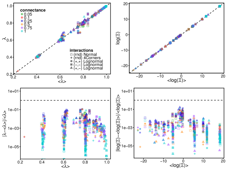
Supplementary Figure S2: Universality of $\lambda$ and $\Xi$ in random matrices. The two left panels refer to the eigenvalue with the largest real part $\lambda$ of the interaction matrix $\boldsymbol{A}$, while the right ones to the size $\Xi$ of the feasibility domain. We consider different values of the connectance (colors) and different distributions (shape), such that there were multiple combination of connectances and distributions having the same values of $E_{1}$, $E_{2}$, and $E_{c}$. We computed the averages $\big{<}\lambda\big{>}$ and $\big{<}\log(\Xi)\big{>}$ over all realizations of the matrices having the same values of $E_{1}$, $E_{2}$, and $E_{c}$. If the value of $\lambda$ and $\Xi$ are universal, then they depend only on $E_{1}$, $E_{2}$, and $E_{c}$, and therefore their values are equal to the mean: universality holds if $\lambda=\big{<}\lambda\big{>}$ and $\log(\Xi)=\big{<}\log(\Xi)\big{>}$. The top panels show that these two quantities are equal and the bottom panels quantify their deviations. We know that $\lambda$ is universal, and since $\Xi$ has a similar behavior, we conclude that $\Xi$ is also universal.

S6 Mean-field approximation of $\Xi$

The goal of this section is to compute an approximation for $\Xi$ in the limit of large $S$. The volume $\Xi$ is defined (see section S4) as

$$\Xi=\frac{2^{S}\ \Gamma(S/2)\ \sqrt{\det(\boldsymbol{G})}}{2\pi^{S/2}}\int_{\mathbb{S}_{S}}\mathrm{d}^{S}\boldsymbol{u}\ \prod_{i=1}^{S}\Theta(u_{i})\ \left(\sum_{i,j}u_{i}G_{ij}u_{j}\right)^{-S/2}\ ,$$ (S55)

where the matrix $\boldsymbol{G}$ can be obtained from the generators of the polytope (see equations S12 and S32), and therefore from the interaction matrix $\boldsymbol{A}$.

We can introduce a Gaussian function in equation S55 using the fact that, for any positive constant $c$,

$$c^{-S/2}=\frac{2}{\Gamma(S/2)}\int_{0}^{\infty}\mathrm{d}r\ r^{S-1}\exp(-cr^{2})\ .$$ (S56)

Introducing this Gaussian integral in equation S55 by letting $c=\sum_{i,j}u_{i}G_{ij}u_{j}$, we obtain

$$\Xi=\sqrt{\det(\boldsymbol{G})}\left(\frac{2}{\sqrt{\pi}}\right)^{S}\int_{0}^{\infty}\mathrm{d}r\ r^{S-1}\int_{\mathbb{S}_{S}}\mathrm{d}^{S}\boldsymbol{u}\ \left(\prod_{i=1}^{S}\Theta(u_{i})\right)\ \exp\left(-r^{2}\sum_{i,j}u_{i}G_{ij}u_{j}\right)\ ,$$ (S57)

which can be rewritten as

$$\Xi=\sqrt{\det(\boldsymbol{G})}\Bigl{(}\frac{2}{\sqrt{\pi}}\Bigr{)}^{S}\int_{\mathbb{R}^{S}}\mathrm{d}^{S}\boldsymbol{z}\ \Bigl{(}\prod_{i=1}^{S}\Theta(z_{i})\Bigr{)}\ \exp\Bigl{(}-\sum_{i,j}z_{i}G_{ij}z_{j}\Bigr{)}\ ,$$ (S58)

where $z_{i}=ru_{i}$. We can rewrite this equation as

$$\begin{split}\Xi=&\sqrt{\det(\boldsymbol{G})}\left(\frac{2}{\sqrt{\pi}}\right)^{S}\int_{\mathbb{R}^{S}}\mathrm{d}^{S}\boldsymbol{z}\ \prod_{i=1}^{S}\left(\Theta(z_{i})\ e^{-z_{i}^{2}}\exp\left(-\sum_{j\neq i}z_{i}G_{ij}z_{j}\right)\right)\ ,\end{split}$$ (S59)

where we used the fact that the diagonal entries of $\boldsymbol{G}$, when expressed in terms of the normalized generators, are equal to one.

The reader familiar with statistical mechanics will notice that equation S59, which can be written as

$$\begin{split}\Xi\propto\int_{\mathbb{R}^{S}}\mathrm{d}^{S}\boldsymbol{z}\ q(\boldsymbol{z})\ \prod_{i=1}^{S}\left(\exp\left(-\sum_{j\neq i}z_{i}G_{ij}z_{j}\right)\right)\ ,\end{split}$$ (S60)

has the form of a partition function. For instance one can recover the Ising model Parisi1998 with the choice $q(\boldsymbol{z})=\prod_{i}\delta(z_{i}^{2}=1)$ or the spherical model Berlin1952 when $q(\boldsymbol{z})=\delta(S-\sum_{i}z_{i}^{2})$. The term $z_{i}G_{ij}z_{j}$ in particular plays the role of the interactions of the system.

Integrals of the form S60 are the most studied objects of statistical mechanics, and yet in most cases are not analytically solvable. There are, on the other hand, many techniques that can be used to obtain good approximations to S60. The most celebrated one is probably the mean-field approximation Parisi1998 and it is the one we are using in this section. In particular, the idea of the mean-field approximation is to replace the interactions of an entity (spins in the case of the Ising model or species in our case) with an average “effective” interaction. This reduces a many-body problem, where all interactions of spins or populations are coupled, into an effective one-body problem.

If the system is large enough (in our case if $S\to\infty$), the mean-field approximation is know to be exact in the case of “fully connected” interactions. In terms of equation S60, this corresponds to a matrix $\boldsymbol{G}$ with the same constant in all its offdiagonal entries. The matrix $\boldsymbol{G}$ is constant when $\boldsymbol{A}$ has constant offdiagonal entries. We will consider therefore the case of $\boldsymbol{A}$’s diagonal entries being equal to $-1$ and its offdiagonal entries to a constant $E_{1}$. Using equation S12, the $i$th component of the $k$th generator is then

$$g^{k}_{i}=-\frac{E_{1}}{1+(S-1)E_{1}^{2}}$$ (S61)

for $i\neq k$, and

$$g^{k}_{k}=\frac{1}{1+(S-1)E_{1}^{2}}\ .$$ (S62)

Using equation S32, we therefore obtain that the diagonal entries of $\boldsymbol{G}$ are equal to $1$, while the offdiagonal ones are constant and equal to

$$G_{ij}=\frac{-2E_{1}+(S-2)E_{1}^{2}}{1+(S-1)E_{1}^{2}}\ .$$ (S63)

We define the constant $\beta$ as

$$\beta=S\frac{-2E_{1}+(S-2)E_{1}^{2}}{1+(S-1)E_{1}^{2}}\ ,$$ (S64)

and therefore we have $G_{ii}=1$ and $G_{ij}=\beta/S$ for $i\neq j$. The determinant of $\boldsymbol{G}$ in this case turns out to be

$$\det(\boldsymbol{G})=\left(1+\frac{S-1}{S}\beta\right)\left(1-\frac{\beta}{S}\right)^{S-1}\approx(1+\beta)e^{-\beta}\ ,$$ (S65)

where the last form holds for large $S$. In this case of constant interactions, we obtain, from equation S59,

$$\begin{split}\Xi=&\sqrt{\det(\boldsymbol{G})}\left(\frac{2}{\sqrt{\pi}}\right)^{S}\int_{\mathbb{R}^{S}}\mathrm{d}^{S}\boldsymbol{z}\ \prod_{i=1}^{S}\left(\Theta(z_{i})\ e^{-z_{i}^{2}}\exp\left(-z_{i}\frac{\beta}{S}\sum_{j\neq i}z_{j}\right)\right)=\\ &=\sqrt{\det(\boldsymbol{G})}\left(\frac{2}{\sqrt{\pi}}\right)^{S}\int_{\mathbb{R}^{S}}\mathrm{d}^{S}\boldsymbol{z}\ \left(\prod_{i=1}^{S}\Theta(z_{i})\right)\ \exp\left(-\sum_{i}z_{i}^{2}-\frac{\beta}{S}(\sum_{i}z_{i})^{2}\right)\ ,\end{split}$$ (S66)

up to subleading terms in $S$.

Equation S66 can be written as

$$\begin{split}\Xi=&\sqrt{\det(\boldsymbol{G})}\left(\frac{2}{\sqrt{\pi}}\right)^{S}Z_{h}\Bigl{\langle}\exp\left(-\frac{\beta}{S}(\sum_{i}z_{i})^{2}+h\sum_{i}z_{i}\right)\Bigr{\rangle}_{h}\ ,\end{split}$$ (S67)

where

$$\begin{split}Z_{h}&:=\int_{\mathbb{R}^{S}}\mathrm{d}^{S}\boldsymbol{z}\ \left(\prod_{i=1}^{S}\Theta(z_{i})\right)\ \exp\left(-\sum_{i}z_{i}^{2}-h\sum_{i}z_{i}\right)=\\ &=\left(\int_{0}^{\infty}\mathrm{d}z\ e^{-z^{2}-hz}\right)^{S}=\left(\frac{\sqrt{\pi}}{2}e^{h^{2}/4}\operatorname{erfc}(h/2)\right)^{S}\ ,\end{split}$$ (S68)

where $\operatorname{erfc}(\cdot)$ is the complementary error function, defined as

$$\operatorname{erfc}(x)=\frac{2}{\sqrt{\pi}}\int_{x}^{\infty}\mathrm{d}t\ e^{-t^{2}}\ .$$ (S69)

The average $\langle\cdot\rangle_{h}$ is defined as

$$\begin{split}\Bigl{\langle}f(\boldsymbol{z})\Bigr{\rangle}_{h}:=\frac{1}{Z_{h}}\int_{\mathbb{R}^{S}}\mathrm{d}^{S}\boldsymbol{z}\ \left(\prod_{i=1}^{S}\Theta(z_{i})\right)\ \exp\left(-\sum_{i}z_{i}^{2}-h\sum_{i}z_{i}\right)f(\boldsymbol{z})\ .\end{split}$$ (S70)

Using Jensen’s inequality in equation S70 we have that

$$\begin{split}\Xi=&\sqrt{\det(\boldsymbol{G})}\left(\frac{2}{\sqrt{\pi}}\right)^{S}Z_{h}\Bigl{\langle}\exp\left(-\frac{\beta}{S}(\sum_{i}z_{i})^{2}+h\sum_{i}z_{i}\right)\Bigr{\rangle}_{h}\geq\\ &\geq\sqrt{\det(\boldsymbol{G})}\left(\frac{2}{\sqrt{\pi}}\right)^{S}Z_{h}\exp\left(\Bigl{\langle}-\frac{\beta}{S}(\sum_{i}z_{i})^{2}+h\sum_{i}z_{i}\Bigr{\rangle}_{h}\right)\ .\end{split}$$ (S71)

In the following we will approximate the first expression with the second one. It is possible to prove that, in the large $S$ limit, the second expression converges to the first one.

Applying the mean-field approximation we neglect fluctuations of the variables, i.e. we have

$$\Bigl{\langle}-\frac{\beta}{S}(\sum_{i}z_{i})^{2}+h\sum_{i}z_{i}\Bigr{\rangle}_{h}=-\frac{\beta}{S}\Bigl{\langle}(\sum_{i}z_{i})^{2}\Bigr{\rangle}_{h}+h\sum_{i}\langle z_{i}\rangle_{h}\approx S\left(-\beta m^{2}+hm\right)\ ,$$ (S72)

where

$$m:=\langle z_{i}\rangle_{h}=-\frac{1}{S}\frac{\partial}{\partial h}\log(Z_{h})\ .$$ (S73)

By introducing equation S72 in equation S71 we have

$$\Xi\approx\sqrt{\det(\boldsymbol{G})}Z_{h}\left(\frac{2}{\sqrt{\pi}}\exp\left(-\beta m^{2}+hm\right)\right)^{S}=\Xi_{MF}\ .$$ (S74)

This equation is a function of $h$, which is a free parameter. Since it is a lower bound for the actual value of $\Xi$, the best approximation would correspond to the value of $h$ which maximizes the approximation. We have therefore that $h$ is a solution of the following equation

$$0=\frac{\partial}{\partial h}\log(\Xi_{MF})=\frac{\partial}{\partial h}\log(Z_{h})+S\frac{\partial}{\partial h}(-\beta m^{2}+hm)=S(h-2\beta m)\frac{\partial m}{\partial h}\ ,$$ (S75)

where $m$ is given by equation S73. We obtain therefore $m=h/(2\beta)$ and then, by neglecting sub-leading terms in $S$ and introducing $m=h/(2\beta)$ in equation S74

$$\frac{1}{S}\log\Xi_{MF}\approx\log\left(\operatorname{erfc}(h/2)\exp\left(\frac{h^{2}}{4}\frac{1+\beta}{\beta}\right)\right)\ .$$ (S76)

By maximizing this equation respect to $h$ we obtain

$$0=\frac{\partial}{\partial h}\log(\Xi_{MF})=\frac{h}{2}\left(\frac{1}{\beta}+1\right)+\frac{\partial}{\partial h}\log\left(\operatorname{erfc}(h/2)\right)=\frac{h}{2}\left(\frac{1}{\beta}+1\right)-\frac{e^{-h^{2}/4}}{\sqrt{\pi}\operatorname{erfc}(h/2)}\ .$$ (S77)

Equation S77 cannot be solved exactly. By expanding around $h=0$ we obtain

$$0=\frac{h}{2}\left(\frac{1}{\beta}+1\right)-\frac{1}{\sqrt{\pi}}-\frac{h}{\pi}\ ,$$ (S78)

which is solved by

$$h=\frac{2\beta\sqrt{\pi}}{\pi+\beta(\pi-2)}\ .$$ (S79)

One can observe that the solution $h=0$ corresponds to $\beta=0$, i.e. to a non-interacting ecosystem. Expanding around $h=0$ is therefore meaningful when the interactions are not too strong. It is possible to verify that the approximate solution S79 is very close to the actual solution obtained by solving numerically equation S77 also for not too small values of $\beta$

Using equation S79 into equation S76 we obtain

$$\frac{1}{S}\log\Xi_{MF}\approx\frac{\beta(1+\beta)\pi}{\left(\pi+\beta(\pi-2)\right)^{2}}+\log\operatorname{erfc}\left(\frac{\sqrt{\pi}\beta}{\pi+\beta(\pi-2)}\right)\ ,$$ (S80)

which is our final result. In figure S3 we compare this equation with the volume computed numerically in the case of constant interactions, finding a very good match.

In the most general case of an interaction matrix with nonconstant offdiagonal entries, we can consider equation S72 as an approximation valid in the case of $E_{2}\to 0$. As $\beta$ was defined in terms of the generators, we can extend the approximation to the case $E_{2}>0$ by considering $\beta$ as the expected value of $\boldsymbol{G}$’s entries, which corresponds to the average overlap of two rows of the interaction matrix $\langle\cos(\eta)\rangle$, defined in equation S116. In this more general case the mean-field value of $\Xi$ is expected to be a good approximation when $\mathrm{var}(\cos(\eta))$ is small enough. By substituting $\beta=\langle\cos(\eta)\rangle$, using equation S119, into equation S72 we obtain

$$\begin{split}\frac{1}{S}\log(\Xi)&\approx\frac{\pi E_{1}(2d-E_{1}S)\left(2dE_{1}+d-S\left(2E_{1}^{2}+E_{2}^{2}\right)\right)}{\left(d(2(\pi-2)E_{1}+\pi)-S\left(2(\pi-1)E_{1}^{2}+\pi E_{2}^{2}\right)\right)^{2}}\\ &\log\left(\operatorname{erfc}\left(\frac{\sqrt{\pi}E_{1}(E_{1}S-2d)}{S\left(2(\pi-1)E_{1}^{2}+\pi E_{2}^{2}\right)-d(2(\pi-2)E_{1}+\pi)}\right)\right)\ .\end{split}$$ (S81)

When $\mathrm{var}(\cos(\eta))$ is not small, we observed that the empirical formula

$$\begin{split}\frac{1}{S}\log(\Xi)&\approx\frac{\pi E_{1}(2d-E_{1}S)\left(2dE_{1}+d-S\left(2E_{1}^{2}+E_{2}^{2}\right)\right)}{\left(d(2(\pi-2)E_{1}+\pi)-S\left(2(\pi-1)E_{1}^{2}+\pi E_{2}^{2}\right)\right)^{2}}\\ &\log\left(\operatorname{erfc}\left(\frac{\sqrt{\pi}E_{1}(E_{1}S-2d)}{S\left(2(\pi-1)E_{1}^{2}+\pi E_{2}^{2}\right)-d(2(\pi-2)E_{1}+\pi)}\right)\right)+\\ &+\log\left(1+\frac{3SE_{2}^{2}(1+E_{c})}{2\pi}\right)\ .\end{split}$$ (S82)

explains well the values obtained in simulations. This is the formula we used to make figure 2 in the main text.

In order to simplify the expression and make it more readable, we can expand equation S80 around $\beta=0$, i.e., when the interactions between species are small. By expanding $(\Xi_{MF})^{1/S}$ around $\beta=0$ and taking the logarithm of the expression, we obtain

$$\frac{1}{S}\log\Xi_{MF}\approx\log\left(1-\frac{\beta}{\pi}\right)\ .$$ (S83)

Equation 2 of the main text was obtained by substituting $\beta=\langle\cos(\eta)\rangle$, using equation S119, in the case of $E_{2}=0$.

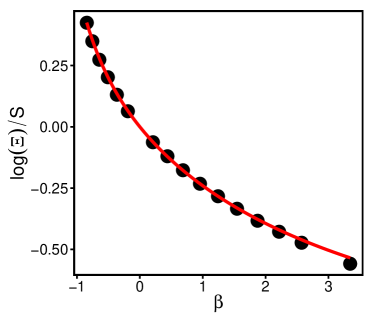
Supplementary Figure S3: Approximation of $\Xi$ using mean field theory. The black dots are numerical simulations obtained by integrating $\Xi$ numerically (see section S4) for a constant interaction matrix. The red curve is the analytical approximation obtained using the mean-field approximation (see equation S81). $\beta$ is a function of $E_{1}$ and $S$, and is defined in equation S64. The range of $\beta$ considered here is the same of the one appearing in figure 1 of the main text.

S7 Feasibility of consumer-resource communities

This section considers explicitly a community with two trophic levels and consumer-resource interactions. While empirical communities have a more complicated interaction structure, this example is particularly relevant to better understand how $\Xi$ should be interpreted.

We consider a system with $S_{R}$ resource and $S_{C}$ consumer ($S_{R}+S_{C}=S$) populations, whose dynamics is described by equation S1 with the interaction matrix

$$\boldsymbol{A}=\left(\begin{array}[]{cc}-\boldsymbol{C}&-\boldsymbol{B}\\ \boldsymbol{Z}\boldsymbol{B}^{T}\boldsymbol{W}&\boldsymbol{0}\\ \end{array}\right)\ ,$$ (S84)

where $\boldsymbol{C}$ is an $S_{R}\times S_{R}$ nonnegative matrix, $\boldsymbol{B}$ is an $S_{R}\times S_{C}$ nonnegative matrix, while $\boldsymbol{Z}$ and $\boldsymbol{W}$ are two positive diagonal matrices of dimension $S_{R}\times S_{R}$ and $S_{C}\times S_{C}$, respectively.

If $\boldsymbol{C}$ is a positive diagonal matrix, any feasible fixed point is globally asymptotically stable Case1979 . When $\boldsymbol{C}$ is not diagonal, one can prove that any feasible fixed point is globally asymptotically stable if $\boldsymbol{C}\boldsymbol{W}^{-1}$ is positive definite (i.e., $-\boldsymbol{C}\boldsymbol{W}^{-1}$ is negative definite). Assuming that this condition holds, stability of feasible fixed points is ensured and we can study feasibility alone.

Using equation S3, we obtain the equations

$$r^{R}_{i}=\sum_{j=1}^{S_{R}}C_{ij}n^{R*}_{j}+\sum_{j=1}^{S_{C}}B_{ij}n^{C*}_{j}\ ,$$ (S85)

$$-r^{C}_{i}=\sum_{j=1}^{S_{R}}Z_{i}B_{ji}W_{j}n^{R*}_{j}\ ,$$ (S86)

where $\boldsymbol{r}^{R}$ and $\boldsymbol{r}^{C}$ are the intrinsic growth rates of resources and consumers, while $\boldsymbol{n}^{R*}$ and $\boldsymbol{n}^{C*}$ are their equilibrium abundances. Since all the matrices that appear in this equation are nonnegative, an intrinsic growth rate vector is contained in the feasibility domain only if $r^{R}_{i}>0$ for all $i=1,\dots,S_{R}$ and $r^{C}_{i}<0$ for all $i=1,\dots,S_{C}$. An intrinsic growth rate vector that does not respect these conditions is not in the feasibility domain. The feasibility domain is therefore fully contained in one orthant, implying that the maximum value of its size is $\Xi=1$.

The $S$-dimensional volume of the feasibility domain is nonzero only if it is defined by $S$ linearly independent generators. The generators of the feasibility domain are proportional to the columns of the interaction matrix. If the interaction matrix has the form of equation S84, $S_{R}$ generators will have the form $\boldsymbol{g}=(\boldsymbol{v},\boldsymbol{0})$, where $\boldsymbol{v}$ has $S_{C}$ components. These generators can be linearly independent only if $S_{R}\geq S_{C}$, and therefore $\Xi>0$ only if $S_{R}\geq S_{C}$. More generally, if $\det(A)=0$, then $\Xi=0$ Haerter2016 .

Assuming that the determinant of $A$ is different from zero, we can use equation S26 obtaining

$$\Xi=\sqrt{\det(\boldsymbol{A})}\left(\frac{2}{\sqrt{\pi}}\right)^{S}\int_{\mathbb{R}^{S}}\mathrm{d}^{S}\boldsymbol{z}\ \left(\prod_{i=1}^{S}\Theta(z_{i})\right)\ \exp\left(\sum_{ij}z_{i}A_{ij}z_{j}\right)\ .$$ (S87)

Given the structure of the matrix $A$, it is convenient to write $\boldsymbol{z}=(\boldsymbol{v},\boldsymbol{u})$, where $\boldsymbol{v}$ and $\boldsymbol{u}$ are two vectors with $S_{R}$ and $S_{C}$ components respectively. The argument of the exponential can be rewritten as

$$\sum_{ij}z_{i}A_{ij}z_{j}=-\sum_{i=1}^{S_{R}}\sum_{j=1}^{S_{R}}v_{i}C_{ij}v_{j}-\sum_{i=1}^{S_{R}}\sum_{j=1}^{S_{C}}v_{i}B_{ij}(1-Z_{i}W_{j})u_{j}\ .$$ (S88)

By integrating over the variables $\boldsymbol{u}$, we finally obtain

$$\Xi=\sqrt{\det(\boldsymbol{A})}\left(\frac{2}{\sqrt{\pi}}\right)^{S}\int_{\mathbb{R}^{S}}\mathrm{d}^{S_{R}}\boldsymbol{v}\ \left(\prod_{i=1}^{S_{R}}\Theta(v_{i})\right)\ \exp\left(\sum_{ij}v_{i}C_{ij}v_{j}\right)\frac{1}{\prod_{j=1}^{S_{C}}\sum_{i=1}^{S_{R}}v_{i}B_{ij}(1-Z_{i}W_{j})}\ .$$ (S89)

Figure S4 shows the size of the feasibility domain of a consumer-resource community, computed using Monte Carlo integration as explained in section S4. We consider an interaction matrix with the structure of equation S84, with a diagonal $\boldsymbol{C}$ (i.e., $C_{ij}=1$ if $i=j$ and zero otherwise) and scalar matrices $\boldsymbol{Z}$ and $\boldsymbol{W}$ (i.e., $Z_{ii}=W_{ii}=\eta$). The elements of the rectangular matrix $\boldsymbol{B}$ were independently drawn from a lognormal distribution with mean $\mu$ and variance $c_{v}^{2}\mu^{2}$, where $c_{v}$ is the coefficient of variation. Since $\boldsymbol{C}$ is equal to the identity matrix, then the interaction matrix is diagonally stable and therefore any feasible point is globally stable Case1979 . Figure S4 shows the effect of $\eta$, $\mu$ and $c_{v}$ on the size $\Xi$ of the feasibility domain. Interestingly, $\eta$ and $\mu$ have a small effect on $\Xi$, while the coefficient of variation has a strong influence on it. It is important to notice that, as explained above, as the interspecific interaction goes to zero (and therefore both $c_{v}$ and $\mu$ tend to zero), $\Xi\to 0$ as well. Note that in this case not all the species are self-regulated ($A_{ii}=0$ for the predators), and therefore in absence of interspecific interactions, $\Xi\neq 1$.

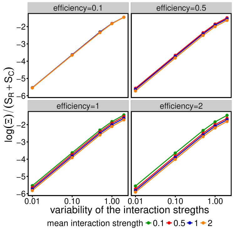
Supplementary Figure S4: Feasibility domain of consumer-resource community. We considered an interaction matrix of the form of equation S84, with $S_{R}=40$ and $S_{C}=30$, $C_{ij}=1$ if $i=j$ and zero otherwise, $Z_{i}W_{j}=\eta>0$ for any $i$ and $j$, and $\boldsymbol{B}$ with entries independently drawn from a Lognormal distribution with mean $\mu$ and variance $c_{v}^{2}\mu^{2}$. For each parameterization we computed the feasibility domain $\Xi$ using the method explained in section S4. The value of $\Xi$ is mostly determined by the coefficient of variation of the interaction, and it depends only weakly on the mean interaction strength $\mu$ and the efficiency $\eta$.

S8 Empirical networks and randomizations

We considered 89 mutualistic networks and 15 food webs. Empirical networks are encoded in terms of adjacency matrices $\boldsymbol{L}$, with $L_{ij}=1$ if species $j$ affects species $i$ and zero otherwise.

S8.1 Mutualistic networks

The 89 mutualistic networks (59 pollination networks and 30 seed-dispersal networks) were obtained from the Web of Life dataset (www.web-of-life.es), where references to the original works can be found. When the original network was not fully connected, we considered the largest connected component.

In the case of mutualistic networks, the adjacency matrix $\boldsymbol{L}$ is bipartite, i.e., it has the structure

$$\boldsymbol{L}=\left(\begin{array}[]{cc}0&\boldsymbol{L}_{b}\\ \boldsymbol{L}_{b}^{T}&0\end{array}\right)\ ,$$ (S90)

where $\boldsymbol{L}_{b}$ is a $S_{A}\times S_{P}$ matrix ($S_{A}$ and $S_{P}$ being the number of animals and plants respectively). The adjacency matrix contains information only about the interactions between animals and plants, but not about competition within plants or animals.

We parameterized the interaction matrix in the following way:

$$\boldsymbol{A}=\left(\begin{array}[]{cc}\boldsymbol{W}^{A}&\boldsymbol{L}_{b}\circ\boldsymbol{W}^{AP}\\ \boldsymbol{L}_{b}^{T}\circ\boldsymbol{W}^{PA}&\boldsymbol{W}^{P}\end{array}\right)\ ,$$ (S91)

where the symbol $\circ$ indicates the Hadamard or entrywise product (i.e., $(\boldsymbol{A}\circ\boldsymbol{B})_{ij}=A_{ij}B_{ij}$), while $\boldsymbol{W}^{A}$, $\boldsymbol{W}^{AP}$, $\boldsymbol{W}^{PA}$, and $\boldsymbol{W}^{P}$ are all random matrices. $\boldsymbol{W}^{A}$ and $\boldsymbol{W}^{P}$ are both square matrices (of dimension $S_{A}\times S_{A}$ and $S_{P}\times S_{P}$), while $\boldsymbol{W}^{AP}$ and $\boldsymbol{W}^{PA}$ are rectangular matrices of size $S_{A}\times S_{P}$ and $S_{P}\times S_{A}$ respectively. The diagonal elements $W^{A}_{ii}$ and $W^{P}_{ii}$ were set to $-1$, while the pairs $(W^{A}_{ij},W^{A}_{ji})$ and $(W^{P}_{ij},W^{P}_{ji})$ were drawn from a bivariate normal distribution with mean $\mu_{-}$, variance $\sigma^{2}_{+}=c\mu_{-}^{2}$, and correlation $\rho\sigma_{+}^{2}$. Since these two matrices represent competitive interactions, $\mu_{-}<0$. The the pairs $(W^{AP}_{ij},W^{PA}_{ji})$ were extracted from a bivariate normal distribution with mean $\mu_{+}$, variance $\sigma_{-}^{2}=c\mu_{+}^{2}$, and correlation $\rho\sigma_{-}^{2}$, where $\mu_{+}>0$.

We analyze more than 600 parameterizations, obtained by considering different values of $\mu_{-}$, $\mu_{+}$, $c$, and $\rho$. For each network and parametrization we computed the size of feasibility domain $\Xi$. The bottom panel of Figure 2 in the main text was obtained by comparing $\Xi$ obtained in this way with the analytical prediction obtained in equation S81.

S8.2 Food webs

A summary of the properties and reference of the food webs can be found in table S1. In the case of food webs the adjacency matrix $L$ is not symmetric, and an entry $L_{ij}=1$ indicates that species $j$ consumes species $i$. We removed all cannibalistic loops. Since both $L_{ij}$ and $L_{ji}$ are never simultaneously equal to one (there are no loops of length two), we parameterized the offdiagonal entries of $\boldsymbol{A}$ as

$$A_{ij}=W^{+}_{ij}L_{ij}+W^{-}_{ji}L_{ji}\ ,$$ (S92)

while the diagonal was fixed at $-1$. Both $\boldsymbol{W}^{+}$ and $\boldsymbol{W}^{-}$ are random matrices, where the pairs $(W^{+}_{ij},W^{-}_{ij})$ are drawn from a bivariate normal distribution with marginal means $(\mu_{+},\mu_{-})$ and correlation matrix

$$\left(\begin{array}[]{cc}c\mu_{+}^{2}&\rho c\mu_{+}^{2}\\ \rho c\mu_{-}^{2}&c\mu_{-}^{2}\end{array}\right)$$ (S93)

We analyzed more than 200 parameterizations, obtained by considering different values of $\mu_{-}$, $\mu_{+}$, $c$, and $\rho$. For each network and parametrization we computed the size of feasibility domain $\Xi$. The bottom panel of Figure 2 in the main text was obtained by comparing $\Xi$ obtained in this way with the analytical prediction obtained in equation S81. In this case the analytical prediction overestimate the actual value of $\Xi$, indicating that there is a role of structure in determining structural stability.

Supplementary Table S1: References and properties of the 15 food webs analyzed in the work

Name	S	Number of links	Connectance
Ythan Estuary DataYthan	92	414	0.1
St. Marks DataStMarks	143	1763	0.17
Grande Cariçaie DataCaricaie	163	2048	0.16
Serengeti DataSerengeti	170	585	0.04
Flensburg Fjord DataFlens	180	1567	0.1
Otago Harbour DataOtago	180	1856	0.12
Little Rock Lake DataLittleRock	181	2316	0.14
Sylt tidal basin DataSylt	230	3298	0.12
Caribbean Reef DataReef	249	3293	0.11
Kongs Fjorden DataKongs	270	1632	0.04
Carpinteria Salt Marsh DataFWPar	273	3878	0.1
San Quintin DataFWPar	290	3934	0.09
Lough Hyne DataLough	349	5088	0.08
Punta Banda DataFWPar	356	5291	0.09
Weddell Sea DataWeddell	488	15435	0.13

S9 Randomization of empirical networks: assessing the role of structure

S9.1 Mutualistic networks

We compared the size of the feasibility domain obtained for empirical networks with the corresponding randomizations. For each network we randomized the block $\boldsymbol{L}_{b}$ 100 times, by generating connected networks with same size and number of links. We parameterized each randomized network independently as described in section S8, and we compared their properties with those of the empirical network, parameterized independently 100 times. Figure S5 shows the comparison between $\Xi$ of random and empirical networks. As expected from the fact that the analytical prediction for random matrices works well, the empirical values and the values obtained with randomizations are compatible. Comparing this figure with figure 2 of the main text we observe that the empirical values and the ones obtained with randomizations match also in the cases were the analytical approximation failed. This implies that the reason of the mismatch is due to the difference between the analytical approximation and the randomizations, and it is not due to the specific structure of the empirical interactions. There are two main sources of errors in this case. On one hand, ours analytical prediction is expected to work is the number of species is large enough and if the variance of interactions is not to high (that is not always true for the parametrizations used). On the other hand, our approximation was formulated for random matrices, while randomizations of mutualistic networks still conserve a bipartite structure.

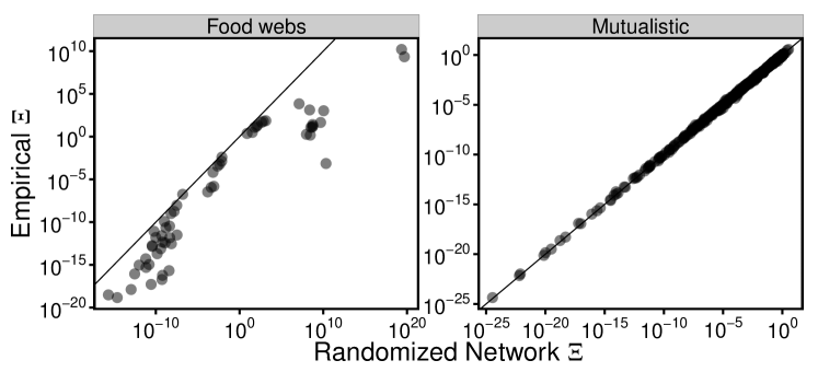
Supplementary Figure S5: Size of feasibility domain $\Xi$ in empirical networks and randomizations. Empirical networks and their randomizations were parametrized as explained in section S8. Each empirical network was parametrized $100$ times and the average $\Xi$ was compared with the one obtained by averaging $100$ randomizations. Each point in this plot correspond therefore to a value of $\Xi$ of an empirical network and its randomizations averaged over the extraction of the interaction strenghts for a given combination of the parameters as explained in section S8.

The randomization procedure explained above and figure S5 show that the size of the coexistence domain obtained with empirical network structure is well predicted by the one obtained with random structure. This result does not imply that structure has no effect on $\Xi$, but it shows that, if this effect exists, it must be relatively small (compared for instance to the variation of $\Xi$ obtained by changing the interaction strengths), i.e. the relative error made by approximating empirical networks with random structure must be small.

Since the effect of structure is small, it is also expected to be very sensible to the interaction strengths. When we parametrized empirical networks and their randomizations to obtain figure S5, we drawn the interaction strengths several times from a given distributions. The realized coefficients were therefore different across different networks, and the values of $\Xi$ shown in figure S5 were averaged over these independent extractions. Since the difference between randomizations and empirical structure is small, it might be impossible to detect any difference with this procedure.

In order to explore and quantify the effect of the empirical structure on the size of feasibility domain, we adopted a different parametrization and randomization method. Given an empirical network, we drawn the interaction strengths only once from a given distribution (as described in section S8). Using this list of interaction strenghts we parametrized $100$ times each empirical network. Different parametrization differ in the position of the coefficients, but not in their values that are conserved across parametrizations. We then compared their size of feasibility domain with the one obtained by parameterizing with the same list of coefficients $100$ randomized networks obtained as explained above.

Figures S6, S7, S8 and S9 show the results obtained for different distributions of interaction strengths (parametrized as explained in section S8). In absence of competition and in absence of variation in the interaction strengths, there is the maximum observable effect. As the competition level is increased and once variation in the interaction strengths is introduced, the effect of the network topology on the total size of feasibility domain becomes negligible.

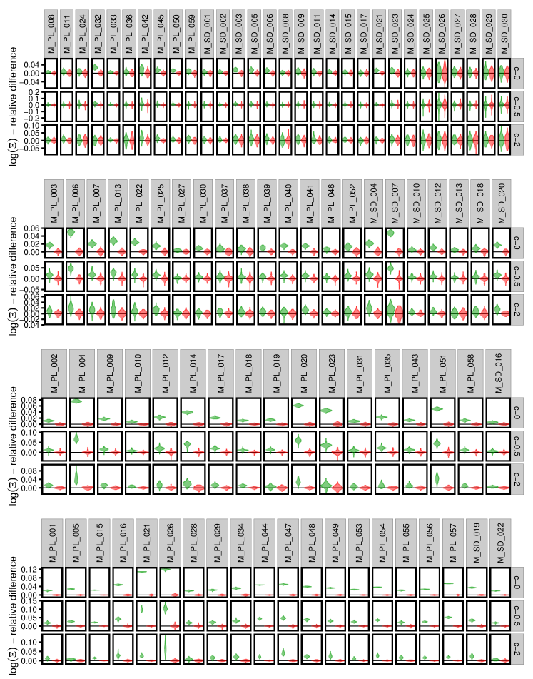
Supplementary Figure S6: We measure the effect of mutualistic network structure on the size of the feasibility domain as described in section S9.1. Red violin plots are randomizations, green ones are empirical networks. The empirical networks are grouped in four rows based on the number of species ($S<50$, $50\leq S<80$, $80\leq S<150$ and $S\geq 150$, respectively). This figure was obtained with $\mu_{+}=0.25\mu_{max}$, $\mu_{-}=0$ and for three different values of $c$.

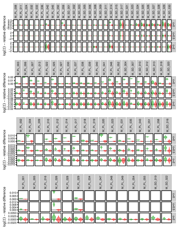
Supplementary Figure S7: Same as figure S6 but with $\mu_{+}=0.25\mu_{max}$ and $\mu_{-}=0.5\mu_{+}$

Supplementary Figure S8: Same as figure S6 but with $\mu_{+}=0.5\mu_{max}$ and $\mu_{-}=0$

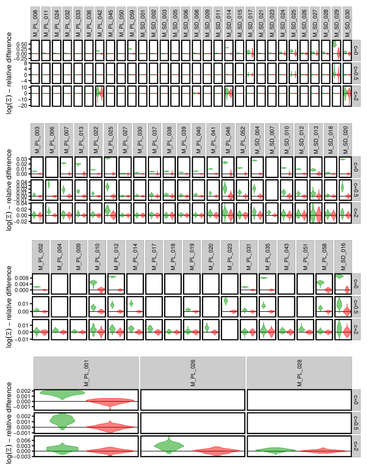
Supplementary Figure S9: Same as figure S6 but with $\mu_{+}=0.5\mu_{max}$ = $\mu_{-}=0.5\mu_{+}$

S9.2 Food webs

We compared the size of feasibility domain of empirical networks with their corresponding randomizations and a network generated accordingly to the cascade modelCohenetal1990 .

For each network, we randomized the adjacency matrix $\boldsymbol{L}$ 100 times, by generating connected networks with the same size and number of links.

We also generated networks generated accordingly to the cascade model (using the same method explained in Allesina2015a ). In this case the adjacency matrix was obtained by generating connected networks with the same size and number of links, by assigning a link between species $i$ and $j$ only if $i>j$.

Figure S10 is the same as figure 2 of the main text, with the addition of randomizations and networks generated with the cascade model. As expected the analytical prediction works very well in describing random networks, while it fails significantly to predict the size of the feasibility domain of cascade and empirical networks. To better quantity the difference between those empirical structures and randomizations, we compared each network separately in figure S11 and S12. We observe that random networks have always larger feasibility domain than networks generated by the cascade model and the empirical ones. Networks generated via the cascade model almost always overestimate the empirical feasibility domains, showing that empirical network structure has a significant negative effect on the size of the feasibility domain.

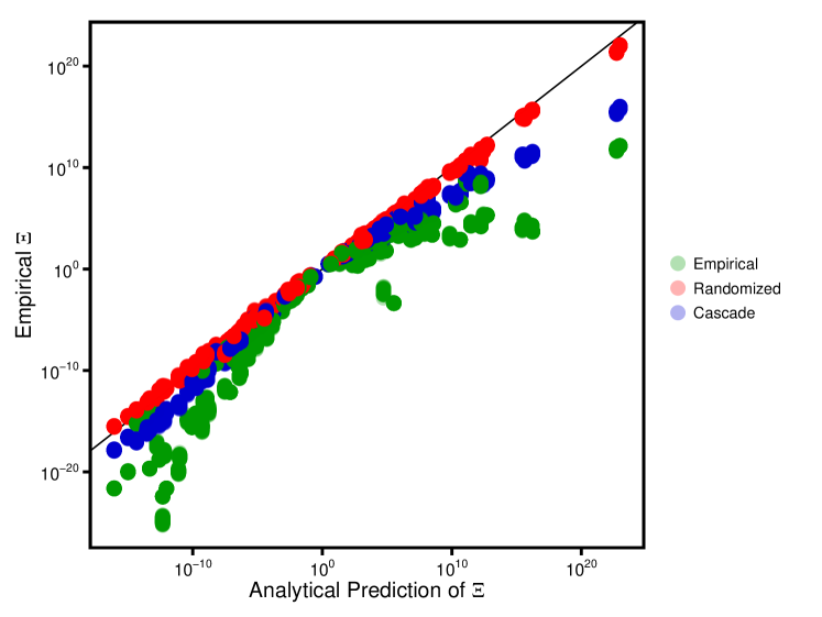
Supplementary Figure S10: In this figure we compared the analytical prediction of the feasibility domain obtained in section S6 with the numerical calculated values for random networks, empirical networks and networks generated via the cascade models. The feasibility domain of random networks is well predicted by our analytical approximation, which fails to predict the empirical one and the one obtained using the cascade model.

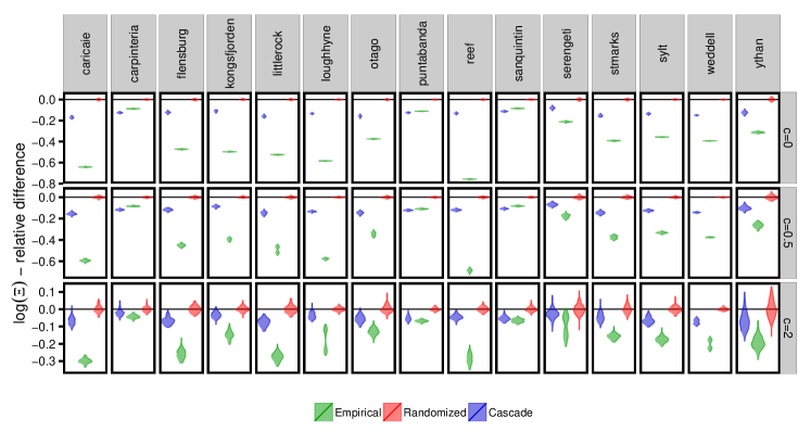
Supplementary Figure S11: We measure the effect of food web network structure on the size of the feasibility domain as described in section S9.2. Red violin plots are randomizations, green ones are empirical networks, while blue ones correspond to the cascade model. This figure was obtained as explained in section S9.2 with $\mu_{-}=0.25\mu_{max}$, $\mu_{+}=0.5\mu_{-}$ and for three different values of $c$.

Supplementary Figure S12: Same as figure S12 but with $\mu_{-}=0.25\mu_{max}$ and $\mu_{+}=2\mu_{-}$

S10  Possible biases in previous analysis of structural stability

In section S4 we showed how to estimate the feasibility domain numerically in a fast and reliable way. In previous approaches Rohr2014 , the feasibility domain (structural stability) was not directly calculated, but approximately inferred using a regression method. In this section we show that the method used by Rohr et al. Rohr2014 could be biased and is not always applicable.

The Authors considered a bipartite mutualistic system described by the dynamical model

$$\left\{\begin{array}[]{cc}\displaystyle\frac{dn^{A}_{i}}{dt}&=\ \displaystyle n^{A}_{i}\left(r_{i}^{A}-\sum_{j=1}^{S_{A}}\beta^{A}_{ij}n^{A}_{j}+\frac{\sum_{j=1}^{S_{P}}\gamma^{A}_{ij}n^{P}_{j}}{1+h_{i}^{A}\sum_{j=1}^{S_{P}}\gamma^{A}_{ij}n^{P}_{j}}\right)\\ \displaystyle\frac{dn^{P}_{i}}{dt}&=\ \displaystyle n^{P}_{i}\left(r_{i}^{P}-\sum_{j=1}^{S_{P}}\beta^{P}_{ij}n^{P}_{j}+\frac{\sum_{j=1}^{S_{A}}\gamma^{P}_{ij}n^{A}_{j}}{1+h_{i}^{P}\sum_{j=1}^{S_{A}}\gamma^{P}_{ij}n^{A}_{j}}\right)\end{array}\right.\ ,$$ (S94)

where $S_{A}$ ($S_{P}$) is the number of animals (plants), and $n^{A}_{i}$ ($n^{P}_{i}$) is the abundance of animal (plant) species $i$. For the purposes of this section we consider the case of linear functional responses $h_{i}^{A}=h_{i}^{P}=0$, as all the methodology used in Rohr2014 was developed in this case. If the functional response is linear, this equation reduces to equation S1, where the interaction matrix $\boldsymbol{A}$ is given by

$$\boldsymbol{A}=\left(\begin{array}[]{cc}-\boldsymbol{\beta}^{A}&\boldsymbol{\gamma}^{A}\\ \boldsymbol{\gamma}^{P}&-\boldsymbol{\beta}^{P}\end{array}\right)\ .$$ (S95)

Here $\boldsymbol{\beta}^{A}$ and $\boldsymbol{\beta}^{P}$ are $S_{A}\times S_{A}$ and $S_{P}\times S_{P}$ matrices, respectively, while $\boldsymbol{\gamma}^{A}$ and $\boldsymbol{\gamma}^{P}$ are $S_{A}\times S_{P}$ and $S_{P}\times S_{A}$ matrices. The Authors used a constant parameterization for the competition parameters, setting $\beta^{A}_{ii}=\beta^{P}_{ii}=1$ and $\beta^{A}_{ij}=\beta^{P}_{ij}=\rho$ if $j\neq i$. The mutualistic benefits were parameterized as

$$\begin{array}[]{cc}\gamma^{A}_{ij}&=\ \displaystyle\gamma_{0}\frac{L_{ij}}{(k_{i}^{A})^{\delta}}\\ \gamma^{P}_{ij}&=\ \displaystyle\gamma_{0}\frac{L_{ji}}{(k_{i}^{P})^{\delta}}\end{array}\ ,$$ (S96)

where $L_{ij}$ is the nonzero block of the adjacency matrix of the interaction network, i.e., $L_{ij}=1$ if there is an interaction between animal $i$ and plant $j$, and zero otherwise. The numbers $k_{i}^{A}=\sum_{j=1}^{S_{P}}L_{ij}$ and $k_{i}^{P}=\sum_{j=1}^{S_{A}}L_{ji}$ are the degree of animal/plant $i$. The two remaining parameters, $\gamma_{0}$ and $\delta$, quantify the levels of mutualistic strength and the mutualistic tradeoff Saavedra2013 .

The method proposed by Rohr et al. Rohr2014 was based on what the Authors called the “structural vector”. It was defined as the center of feasibility domain and was calculated by transforming the mutualistic dynamics into an effective competitive one. Using this effective dynamics it was possible to calculate an effective structural vector, which was then transformed back to the one of the mutualistic system. Starting from the structural vector, the Authors considered different perturbations of the growth rates by changing their direction from that of the original structural vector by some given angle. The dynamics was then integrated and the probability that all species survived was calculated, given a particular perturbation. Running this across several different perturbations and parameterizations, it was possible to perform a regression between the interaction parameters, the angle by which the growth rates were perturbed, nestedness, and other parameters appearing in the interaction matrix. Using the coefficients obtained through the regression, it was quantified the effect of nestedness and other properties on the size of the feasibility domain. Here we present some possible issues emerging from this approach.

It is not always possible to find the structural vector. In order to calculate the structural vector, one needs to transform the mutualistic system into an effective competitive one. One can define the matrix $\boldsymbol{T}=\boldsymbol{1}+\boldsymbol{\gamma}\boldsymbol{\beta}^{-1}$, where $\boldsymbol{1}$ is the identity matrix and

$$\boldsymbol{\beta}=\left(\begin{array}[]{cc}\boldsymbol{\beta}^{A}&0\\ 0&\boldsymbol{\beta}^{P}\end{array}\right)\ ,$$ (S97)

and

$$\boldsymbol{\gamma}=\left(\begin{array}[]{cc}0&\boldsymbol{\gamma}^{A}\\ \boldsymbol{\gamma}^{P}&0\end{array}\right)\ .$$ (S98)

By multiplying both sides of equation S95 by $\boldsymbol{T}$ one obtains the effective interaction matrix

$$\boldsymbol{A}_{\text{eff}}=\left(\begin{array}[]{cc}-\boldsymbol{\beta}^{A}+\boldsymbol{\gamma}^{P}(\boldsymbol{\beta}^{P})^{-1}\boldsymbol{\gamma}^{A}&0\\ 0&-\boldsymbol{\beta}^{P}+\boldsymbol{\gamma}^{A}(\boldsymbol{\beta^{A}})^{-1}\boldsymbol{\gamma}^{P}\end{array}\right)=:\left(\begin{array}[]{cc}\boldsymbol{B}_{\text{eff}}^{A}&0\\ 0&\boldsymbol{B}_{\text{eff}}^{P}\end{array}\right)\ ,$$ (S99)

In order to calculate the structural vectors, one has to assume that the eigenvectors associated with the largest singular eigenvalues of $(\boldsymbol{B}_{\text{eff}}^{A})^{T}\boldsymbol{B}_{\text{eff}}^{A}$ and $\boldsymbol{B}_{\text{eff}}^{A}(\boldsymbol{B}_{\text{eff}}^{A})^{T}$ have only positive components (and an equivalent condition on $\boldsymbol{B}_{\text{eff}}^{P}$ ). This is not generally true, as also stated by the Authors Rohr2014 . They therefore imposed the extra assumption that $(\boldsymbol{B}_{\text{eff}}^{A})^{T}\boldsymbol{B}_{\text{eff}}^{A}$ and $\boldsymbol{B}_{\text{eff}}^{A}(\boldsymbol{B}_{\text{eff}}^{A})^{T}$ indeed have only positive entries (and the equivalent conditions on $\boldsymbol{B}_{\text{eff}}^{P}$). In this case, the Perron–Frobenius theorem allows all entries of the leading eigenvector to be chosen positive; i.e., it necessarily points in some feasible direction. The Authors then identified the structural vectors with these eigenvectors.

However, the extra requirement that $(\boldsymbol{B}_{\text{eff}}^{A})^{T}\boldsymbol{B}_{\text{eff}}^{A}$ and $\boldsymbol{B}_{\text{eff}}^{A}(\boldsymbol{B}_{\text{eff}}^{A})^{T}$ be strictly positive imposes constraints on the interaction matrix that reduces the number of parameterizations that can be analyzed with this method. Since this assumption does not hold in general, there are cases in which the structural vector does not exist. Using our approach, this vector is not needed (see sections S4 and S11).

When the structural vector exists, it is not unique. Under what conditions would the matrices $(\boldsymbol{A}^{\text{eff}})^{T}\boldsymbol{A}^{\text{eff}}$ and $\boldsymbol{A}^{\text{eff}}(\boldsymbol{A}^{\text{eff}})^{T}$ satisfy the conditions of the Perron–Frobenius theorem? It is easy to show that this can never be the case. From equation S99 we see that $\boldsymbol{A}^{\text{eff}}$ is block-diagonal, therefore $(\boldsymbol{A}^{\text{eff}})^{T}\boldsymbol{A}^{\text{eff}}$ and $\boldsymbol{A}^{\text{eff}}(\boldsymbol{A}^{\text{eff}})^{T}$ are block-diagonal as well. This means that the Perron–Frobenius theorem does not hold (the matrix is reducible); instead, the two diagonal blocks each have an all-positive leading eigenvector (assuming that all the coefficients are positive in the two blocks). Any linear combination of the two will have positive components. There is no reason to prefer one linear combination over another, and while it is true that some linear combinations may point closer to the center of the feasibility domain, there is no way to determine using the Authors’ methods which combination does, if any.

The structural vector is not the center of the feasibility domain. Let us assume now that the structural vector exists and it points toward the center of the feasibility domain of the effective competitive system. To obtain the structural vector, one has to transform it back to a vector of the original, mutualistic system. The transformation from the effective to the original system is done by multiplying with the matrix $\boldsymbol{T}^{-1}$. This matrix is not a rotation, and therefore it does not preserve the angles between vectors. Even if a vector is the center of the feasibility domain in the effective system, it will not in general be the center of the original domain. In particular, its distance to the actual center of the original domain will be dependent on parameterization and network structure, as the transformation matrix depends on these.

In contrast, the center of the feasibility domain can be easily expressed with our approach in terms of the matrix $\boldsymbol{A}$ and its associated generators (section S3, equation S20). It is also easy to check that the barycenter is different from the one obtained using the method of Rohr et al. Rohr2014 .

The regression procedure can in principle produce biases. The relationship between network structure and the size of the feasibility domain was obtained by calculating the probability of coexistence $p(\theta_{A},\theta_{P})$, where $\theta_{A/P}$ is the angle by which the direction of the growth rate vector of animals/plants was changed with respect to the structural vector. The Authors then performed a linear regression

$$\begin{split}\text{logit}(p(\theta_{A},\theta_{P}))&\sim\beta_{1}\log\theta_{A}+\beta_{2}\log\theta_{B}+\beta_{3}\gamma_{0}C+\beta_{4}\gamma_{0}^{2}C^{2}\\ &+\beta_{5}\gamma_{0}CN+\beta_{6}\gamma_{0}CN^{2}+\beta_{7}\gamma_{0}C\delta+\beta_{8}\gamma C\delta^{2}\ ,\end{split}$$ (S100)

where $C$ is the connectance of the mutualistic adjacency matrix and $N$ is its nestedness (note that $\bar{\gamma}$, used by Rohr et al. Rohr2014 , is equal to $C\gamma_{0}$). The fitted parameters where then used to determine the effect of nestedness and other quantities on the feasibility domain. The functional dependence assumed above cannot be justified a priori, and an incorrect functional dependence can in principle lead to erroneous fitting results. For instance, the effect of those properties could be different depending not just on the raw angle of perturbation, but also which direction that angle is taken in. We can imagine two feasibility regions with the exact same size but different shapes: one of the two is equally wide in all directions, while the other stretches very wide in some directions but is extremely narrow in others (see section S11). For sufficiently small values of $\theta_{A/P}$, one will never leave the feasible domain in the first of these examples, but may do so in the second if the perturbation is performed in one of the “narrow” directions. The first of these cases will therefore appear more feasible than the second, even though the total size of the two feasibility regions is in fact the same. On the other hand, if the values of $\theta_{A/P}$ are large enough, than the perturbed vector in the first case will never be feasible, while it will be feasible in the second case because of the “wide” directions. Moreover, this method does not allow one to calculate the feasibility domain for a given network and parameterization, as one can calculate only the probability of coexistence given an angle of perturbation.

S11  Distribution of side lengths

In section S3 we showed that the feasibility domain is a convex polyhedral cone in the space of intrinsic growth rates $\boldsymbol{r}$. Since the stationary solution of equation S1 is linear in $\boldsymbol{r}$, we can study the feasibility domain considering only vectors on the unit sphere’s surface. In section S4 we defined $\Xi$, which quantifies the volume of the feasibility domain.

The size of the feasibility domain, i.e., how many combinations of the intrinsic growth rates correspond to a feasible fixed point, is not the only interesting property. Two systems having the same number of feasible combinations of growth rates (i.e., the same value of $\Xi$), can respond very differently to perturbations of the growth rates. We imagine here that a perturbation (e.g., a change of the abiotic conditions) correspond to a change in the growth rate vector. Since we can consider normalized growth rate vectors (because of the linearity of the equations), the effect of a perturbation on feasibility depends only on the angular change of the growth rate vector and not on its length.

The volume $\Xi$ quantifies how many growth rate vectors are compatible with coexistence. Let us consider a feasible growth rate vector, and perturb it in a random direction. What is the probability that the new vector is still feasible? This is not just a function of the size $\Xi$ of the feasibility domain. Indeed, one can imagine that the feasibility domain is about equally spread in every direction—or that, for the exact same value of $\Xi$, the feasibility domain is streched in some directions but is very narrow in some other ones. A perturbation in one of the “narrow” directions is much more likely to lead out of the feasibility domain in the latter case than in the former.

To quantify this property, one strategy could be to measure the different responses on the perturbation (i.e., the probability of being feasible) depending on the direction of the perturbation (in which direction we change the growth rate vector). This choice has the big disadvantage of depending not only on the properties of interactions (the interaction matrix $\boldsymbol{A}$), but also on the strength of the perturbation (the angular displacement between the initial and the final growth rate vector) and the growth rate vector before the perturbation (e.g., if the initial vector is close or far from the edge of the feasibility domain). We propose instead a purely geometrical method to quantify the response to different perturbations (see figure 1 of the main text).

The feasibility domain, when restricted to the surface of a hypersphere, can be imagined as the generalization of a triangle on a sphere (see section S13). The natural, geometric quantities bounding the maximal perturbation that will leave the system feasible, are the lengths of the triangle’s sides. When $S$ species are considered, there are $S(S-1)/2$ sides. Their lengths measure the maximum permissible perturbation of the growth rates in the corresponding direction if one is to retain feasibility. This property has the advantage of being purely geometrical, depending only on the interactions (via the interaction matrix) and not, for instance, on any choice of the initial conditions.

We can measure the distribution of the side lengths. Imagine we have two interaction matrices with the same $\Xi$, but with very different distributions of side lengths. One of them has all sides of equal length, while the other one has a more heterogeneous distribution. In the first case any direction of the perturbation is expected to have a similar effect, and there are no particularly dangerous directions. In the second case there are some directions of the perturbation that are much more dangerous than others, and even a small change of conditions along one of those dangerous direction can lead to the extinction of one or more species.

We know that the feasibility domain is a convex polyhedral cone (see section S3). Its “corners” are identified by its generators and its sides are determined by all pairs of generators (see section S13 for the $S=3$ case).

Since we are considering growth rates on the unit (hyper)sphere, and the generators are normalized to one, any pair of generators will lie on the sphere’s surface. The scalar product of two generators is the cosine of the angle between the two. Since the two generators are on the unit ball’s surface, the arc between the two (which is the side length) is equal to the angle. We have therefore that the length of the side of the feasibility domain corresponding to a pair of generators $\boldsymbol{g}^{i}$ and $\boldsymbol{g}^{j}$ is

$$\eta_{ij}=\arccos\left(\boldsymbol{g}^{i}\cdot\boldsymbol{g}^{j}\right)\ .$$ (S101)

Using equation S12, we can express the $S(S-1)/2$ side lengths of the convex polytope explicitly in terms of the interaction matrix:

$$\eta_{ij}=\arccos\left(\frac{\sum_{k}A_{ki}A_{kj}}{\sqrt{\sum_{k}A_{ki}A_{ki}\sum_{l}A_{lj}A_{lj}}}\right)\ .$$ (S102)

We are interested in the distribution of the side lengths, and in particular in its heterogeneity. In the following section we will calculate these quantities for random matrices.

S11.1  The distribution of side lengths in random matrices

In this section we obtain the distribution of sides length for large random matrices, whose entries are distributed accordingly to an arbitrarily bivariate distribution.

We assume that the diagonal elements of $\boldsymbol{A}$ are all equal to $-d$ (this hypothesis can be easily generalized), while the offdiagonal pairs $(A_{ij},A_{ji})$ are random variables with distribution $q(x,y)$. Our goal is to find the distribution of the side lengths $\eta$ in the large $S$ limit, defined as

$$\begin{split}P(\eta)=&\lim_{S\to\infty}\frac{1}{S(S-1)}\sum_{i\neq j}\int\prod_{m>n}\Bigl{(}\mathrm{d}A_{mn}\mathrm{d}A_{nm}q(A_{mn},A_{nm})\Bigr{)}\\ \times&\ \delta\left(\eta-\arccos\left(\frac{\sum_{k}A_{ki}A_{kj}}{\sqrt{\sum_{k}A_{ki}A_{ki}\sum_{l}A_{lj}A_{lj}}}\right)\right),\end{split}$$ (S103)

Since we are summing over all $i$ and $j$, and all the rows are identically distributed, we can remove the sum and consider just two rows:

$$\begin{split}P(\eta)=&\lim_{S\to\infty}\int\prod_{m>n}\Bigl{(}\mathrm{d}A_{mn}\mathrm{d}A_{nm}q(A_{mn},A_{nm})\Bigr{)}\\ \times&\ \delta\left(\eta-\arccos\left(\frac{\sum_{k}A_{k1}A_{k2}}{\sqrt{\sum_{k}A_{k1}A_{k1}\sum_{l}A_{l2}A_{l2}}}\right)\right),\end{split}$$ (S104)

Since we are interested in the large $S$ limit, we have that

$$\begin{split}\sum_{k}A_{k1}A_{k1}=&A_{11}+\sum_{k>1}(A_{k1})^{2}\approx-d+(S-1)\int\mathrm{d}x\mathrm{d}y\ q(x,y)\ x^{2}\\ =&-d+(S-1)(E_{1}^{2}+E_{2}^{2}),\end{split}$$ (S105)

where $E_{1}$ and $E_{2}$ are the first and second marginal moments of $q$ (equations S35 and S36). Let us call this quantity $Z$. In this limit we therefore obtain

$$\begin{split}P(\eta)=&\lim_{S\to\infty}\int\prod_{m>n}\Bigl{(}\mathrm{d}A_{mn}\mathrm{d}A_{nm}q(A_{mn},A_{nm})\Bigr{)}\ \delta\left(\eta-\arccos\left(\frac{\sum_{k}A_{k1}A_{k2}}{Z}\right)\right)\\ =&\lim_{S\to\infty}\int\prod_{m>n}\Bigl{(}\mathrm{d}A_{mn}\mathrm{d}A_{nm}q(A_{mn},A_{nm})\Bigr{)}\ Z\ |\sin(\eta)|\ \delta\left(Z\cos(\eta)-\sum_{k}A_{k1}A_{k2}\right)\\ =&\ Z|\sin(\eta)|\lim_{S\to\infty}\int\prod_{m>n}\Bigl{(}\mathrm{d}A_{mn}\mathrm{d}A_{nm}q(A_{mn},A_{nm})\Bigr{)}\ \delta\left(Z\cos(\eta)-\sum_{k}A_{k1}A_{k2}\right)\\ =&\ Z|\sin(\eta)|\lim_{S\to\infty}\int\prod_{m>n}\Bigl{(}\mathrm{d}A_{mn}\mathrm{d}A_{nm}q(A_{mn},A_{nm})\Bigr{)}\\ &\times\delta\left(Z\cos(\eta)-A_{11}A_{21}-A_{22}A_{12}-\sum_{k>2}A_{k1}A_{k2}\right)\\ =&\ Z|\sin(\eta)|\lim_{S\to\infty}\int\prod_{m>n}\Bigl{(}\mathrm{d}A_{mn}\mathrm{d}A_{nm}q(A_{mn},A_{nm})\Bigr{)}\\ &\times\delta\left(Z\cos(\eta)+d(A_{12}+A_{21})-\sum_{k>2}A_{k1}A_{k2}\right)\\ =&\ Z|\sin(\eta)|\int\mathrm{d}t\int\mathrm{d}s\int\mathrm{d}A_{12}\mathrm{d}A_{21}q(A_{12},A_{21})\delta(t-A_{12}-A_{21})\\ &\times\int\prod_{k>2}\mathrm{d}A_{k1}\mathrm{d}A_{k2}q(A_{k1})q(A_{k2})\delta\left(s-\sum_{k>2}A_{k1}A_{k2}\right)\\ &\times\delta\left(Z\cos(\eta)+dt-\sum_{k>2}A_{k1}A_{k2}\right)\\ =&\ Z|\sin(\eta)|\int\mathrm{d}t\int\mathrm{d}s\int\mathrm{d}x\mathrm{d}y\ q(x,y)\delta(t-(x+y))\\ &\times\int\left(\prod_{k=1}^{S-2}dz_{k}dw_{k}q(z_{k})q(w_{k})\right)\delta\left(s-\sum_{k=1}^{S-2}z_{k}w_{k}\right)\delta(Z\cos(\eta)+dt-s)\ ,\end{split}$$ (S106)

where $q(z)$ is the marginal distribution of $q(x,y)$:

$$q(z)=\int\mathrm{d}x\ q(x,z)=\int\mathrm{d}x\ q(z,x).$$ (S107)

We can introduce the distribution of the sum:

$$q_{s}(t)=\int\mathrm{d}x\mathrm{d}\ yq(x,y)\delta(t-(x+y)).$$ (S108)

The term

$$\int\left(\prod_{k=1}^{S-2}\mathrm{d}z_{k}\mathrm{d}w_{k}\ q(z_{k})q(w_{k})\right)\ \delta\left(s-\sum_{k=1}^{S-2}z_{k}w_{k}\right)$$ (S109)

is the distribution of a sum of $S-2$ uncorrelated random variables. These random variables are the product $zw$ of two random variables whose distribution is $q$. Since the second moment of $q(x)$ is finite, the central limit theorem holds and this distribution converges, in the large $S$ limit, to a Gaussian distribution with mean

$$S\int\mathrm{d}x\mathrm{d}y\ q(y)q(x)\ xy=SE_{1}^{2}$$ (S110)

and variance

$$S\left(\int\mathrm{d}x\mathrm{d}y\ q(y)q(x)\ (xy)^{2}-E_{1}^{2}\right)=SE_{2}^{4}\ .$$ (S111)

We have therefore

$$\begin{split}P(\eta)=&\ Z|\sin(\eta)|\int\mathrm{d}t\mathrm{d}s\ q_{s}(t)\frac{\exp\left(\frac{-(s-SE_{1}^{2})^{2}}{2SE_{2}^{4}}\right)}{\sqrt{2S\pi}E_{2}^{2}}\delta(Z\cos(\eta)+dt-s)=(S(E_{1}^{2}+E_{2}^{2})-d)\\ &\times\frac{|\sin(\eta)|}{\sqrt{2S\pi}E_{2}^{2}}\int\mathrm{d}t\ q_{s}(t)\exp\left(-\frac{\big{(}S(E_{1}^{2}+E_{2}^{2})\cos(\eta)-d\cos(\eta)-SE_{1}^{2}+dt\big{)}^{2}}{2SE_{2}^{4}}\right)\ .\end{split}$$ (S112)

The distribution of $\eta$ is not universal as it depends on $q_{s}(t)$, which depends on the distribution of the coefficients. On the other hand, the dependence is explicit, and it is possible to calculate $P(\eta)$ for any distribution $q(x,y)$.

We show explicitly the case of $q(x,y)$ being a bivariate normal distribution, i.e.,

$$q(x,y)=\frac{1}{2\pi E_{2}^{2}\sqrt{1-E_{c}^{2}}}\exp\left(-\frac{(x-E_{1})^{2}+(y-E_{1})^{2}-2E_{c}(x-E_{1})(y-E_{1})}{2E_{2}^{2}}\right)\ .$$ (S113)

In this case $q_{s}(t)$ is a normal distribution, and can be obtained from eq S108

$$\begin{split}q_{s}(t)&=\frac{1}{2\pi E_{2}^{2}\sqrt{1-E_{c}^{2}}}\int\mathrm{d}y\exp\left(-\frac{(t-y-E_{1})^{2}+(y-E_{1})^{2}-2E_{c}(t-y-E_{1})(y-E_{1})}{2E_{2}^{2}}\right)\\ &=\exp\left(-\frac{(1-E_{c})(t-2E_{1})^{2}}{4E_{2}^{2}}\right)\frac{1}{2\sqrt{\pi}E_{2}(1+E_{c})\sqrt{1-E_{c}}}\ .\end{split}$$ (S114)

Substituting into equation S112, we see that $P(\eta)$ has the form of a convolution of two Gaussians, and turns out to be equal to

$$\begin{split}P(\eta)=\frac{|\sin(\eta)|}{\sqrt{2\pi}\,\mathrm{var}(\cos(\eta))}\exp\left(-\frac{\big{(}\cos(\eta)-\langle\cos(\eta)\rangle\big{)}^{2}}{2\,\mathrm{var}(\cos(\eta))}\right)\ .\end{split}$$ (S115)

The mean $\langle\cos(\eta)\rangle$ and variance $\mathrm{var}(\cos(\eta))$ will be computed in the next section in the most general case of an arbitrary interaction distribution.

S11.2  Moments for random matrices

As explained in the previous section, the distribution of the side lengths is not a universal quantity, as it depends on the distribution of interaction strengths. In this section we compute the mean and the variance in the general case, showing that they depends only on $E_{1}$, $E_{2}$ and $E_{c}$.

Here and in the main text we do not report the moments of the side length $\eta$, but the moments of its cosine. The cosine of the side length measures the overlap between two rows of the interaction matrix (or the scalar product of two generators of the convex polytope). As its value gets close to one, the side length approaches zero.

Starting from equation S102, we have that

$$\big{<}\cos(\eta)\big{>}=\frac{1}{S(S-1)}\sum_{i\neq j}\cos(\eta_{ij})=\frac{1}{S(S-1)}\sum_{i\neq j}\left(\frac{\sum_{k}A_{ik}A_{jk}}{\sqrt{\sum_{k}A_{ik}A_{ik}\sum_{l}A_{jl}A_{jl}}}\right),$$ (S116)

Since we are interested in the large $S$ limit, we can write the denominator as in equation S105 and obtain

$$\big{<}\cos(\eta)\big{>}=\frac{1}{S(S-1)}\sum_{i\neq j}\left(\frac{\sum_{k}A_{ik}A_{jk}}{-d+S(E_{1}^{2}+E_{2}^{2})}\right)\ ,$$ (S117)

and then

$$\big{<}\cos(\eta)\big{>}=\frac{1}{S(S-1)}\sum_{i\neq j}\left(\frac{A_{ii}A_{ji}+A_{ij}A_{jj}+\sum_{k\neq i,j}A_{ik}A_{jk}}{-d+S(E_{1}^{2}+E_{2}^{2})}\right)\ .$$ (S118)

In the large $S$ limit, this becomes

$$\big{<}\cos(\eta)\big{>}=\frac{-2dE_{1}+SE_{1}^{2}}{-d+(S-2)(E_{1}^{2}+E_{2}^{2})}$$ (S119)

to leading order in $S$.

In a similar way, we can write the second moment as

$$\big{<}\cos(\eta)^{2}\big{>}=\frac{1}{S(S-1)}\sum_{i\neq j}\cos(\eta_{ij})^{2}=\frac{1}{S(S-1)}\sum_{i\neq j}\left(\frac{\sum_{k}A_{ik}A_{jk}}{\sqrt{\sum_{k}A_{ik}A_{ik}\sum_{l}A_{jl}A_{jl}}}\right)^{2}.$$ (S120)

In the large $S$ limit we obtain

$$\begin{split}\big{<}&\cos(\eta)^{2}\big{>}=\frac{1}{S(S-1)}\sum_{i\neq j}\frac{\Bigl{(}\sum_{k}A_{ik}A_{jk}\Bigr{)}^{2}}{\Bigl{(}-d+S(E_{1}^{2}+E_{2}^{2})\Bigr{)}^{2}}=\frac{1}{S(S-1)}\sum_{i\neq j}\frac{\sum_{k}\sum_{l}A_{ik}A_{jk}A_{il}A_{jl}}{\Bigl{(}-d+S(E_{1}^{2}+E_{2}^{2})\Bigr{)}^{2}}\\ &=\frac{1}{S(S-1)}\sum_{i\neq j}\frac{\big{(}A_{ii}A_{ji}+A_{ij}A_{jj}+\sum_{k\neq i,j}A_{ik}A_{jk}\big{)}\big{(}A_{ii}A_{ji}+A_{ij}A_{jj}+\sum_{l\neq i,j}A_{il}A_{jl}\big{)}}{\Bigl{(}-d+S(E_{1}^{2}+E_{2}^{2})\Bigr{)}^{2}}\\ &=\frac{1}{S(S-1)}\sum_{i\neq j}\frac{d^{2}(A_{ij}+A_{ji})^{2}-2d(A_{ij}+A_{ji})\sum_{k\neq i,j}A_{ik}A_{jk}+(\sum_{k\neq i,j}A_{ik}A_{jk})^{2}}{\Bigl{(}-d+S(E_{1}^{2}+E_{2}^{2})\Bigr{)}^{2}}\ .\end{split}$$ (S121)

We can compute the averages of the different terms, obtaining

$$\begin{split}\frac{1}{S(S-1)}\sum_{i\neq j}(A_{ij}+A_{ji})^{2}=&\ \frac{1}{S(S-1)}\sum_{i\neq j}(A_{ij}^{2}+A_{ji}^{2}+2A_{ji}A_{ji})\\ =&\ 2(E_{1}^{2}+E_{2}^{2})+2(E_{c}E_{2}^{2}+E_{1}^{2})=4E_{1}^{2}+2(1+E_{c})E_{2}^{2}\ ,\end{split}$$ (S122)

$$\begin{split}\frac{1}{S(S-1)}\sum_{i\neq j}(A_{ij}+A_{ji})\sum_{k\neq i\neq j}A_{ik}A_{jk}&=\frac{1}{S(S-1)}\sum_{i\neq j}(A_{ij}+A_{ji})(S-2)E_{1}^{2}\\ &=2(S-2)E_{1}^{3}\ ,\end{split}$$ (S123)

and

$$\begin{split}\frac{1}{S(S-1)}\sum_{i\neq j}\left(\sum_{k\neq i\neq j}A_{ik}A_{jk}\right)^{2}&=\frac{1}{S(S-1)}\sum_{i\neq j}\sum_{k\neq i,j}\sum_{l\neq i,j}A_{ik}A_{il}A_{jk}A_{jl}\\ &=\frac{1}{S(S-1)}\sum_{i\neq j}\sum_{k\neq i,j}\left(\sum_{l\neq i,j,k}(A_{ik}A_{il}A_{jk}A_{jl})+A_{ik}^{2}A_{jk}^{2}\right)\\ &=(S-2)(S-3)E_{1}^{4}+(S-2)(E_{1}^{2}+E_{2}^{2})^{2}\ .\end{split}$$ (S124)

We finally get that, in the large $S$ limit,

$$\mathrm{var}(\cos(\eta))=\big{<}\cos(\eta)^{2}\big{>}-\big{<}\cos(\eta)\big{>}^{2}=\frac{2d^{2}(1+E_{c})E_{2}^{2}+S(E_{2}^{2}+E_{1}^{2})^{2}-SE_{1}^{4}}{\left(-d+S(E_{1}^{2}+E_{2}^{2})\right)^{2}}\ .$$ (S125)

S12  Side heterogeneity for different structures and empirical networks

In figure S13 we considered the effect of four nonrandom structures on the mean and variance of the side lengths. The interaction strengths were drawn from a normal distribution with given mean, variance, and correlation. For some structures we considered multiple interaction types and therefore multiple means (one positive and one negative), in which case the coefficient of variation of the interactions and the correlation was constant and independent of the mean. Networks were parametrized as explained in section S8.

• Modular. In this case we considered interaction matrices with a perfect block structure (to generate figure 3 we considered four blocks of equal size).

• Bipartite. In this case we considered an interaction matrix with two bipartite blocks of equal size. The mean interaction of the offdiagonal blocks was set to be negative, while the one of the in-diagonal blocks was positive.

• Nested. The interaction matrix had a bipartite structure. The diagonal blocks had a random structure with negative mean interaction strength. In the offdiagonal blocks, we consider a connectance equal to one half and we built a perfectly nested matrix. The mean interaction strength was positive in the offdiagonal blocks.

• Cascade. We build a matrix using the cascade model, and parameterize it with a positive and a negative mean depending on the role of the species in the interaction.

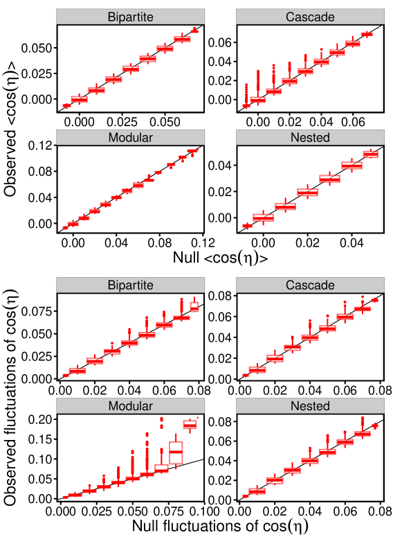
Supplementary Figure S13: We measure the effect of non random structures of mean and variance of side lengths. With the exception of the cascade model, all the structures considered do not have an important effect on $\langle\cos(\eta)\rangle$. On the other side, all the non-random structures considered have a positive effect on the fluctuations of $\cos(\eta)$. All the networks considered had a connectance $C=0.2$.

In the case of empirical structures, figure 3 of the main text, was obtained considering the same networks and the same parameterizations considered in section S8. We compared $\mathrm{var}(\cos(\eta))$ with the values expected in the random case. Figure S14 shows the comparison between $\big{<}\cos(\eta)\big{>}$ obtained for empirical networks with the null prediction. Its value is well predicted by the null expectation for mutualistic networks, while the null expectations underestimates this value for food webs. This is consistent with the fact that the size of feasibility domain of random networks is larger that the one of empirical networks.

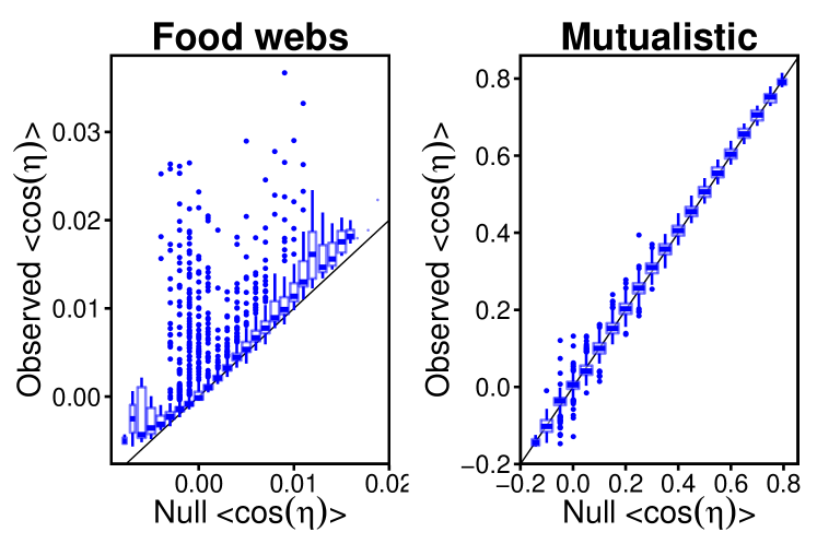
Supplementary Figure S14: Comparision between $\big{<}\cos(\eta)\big{>}$ obtained for empirical networks and its null expectation for empirical food webs and mutualistic networks. This figure was realized with the same parametrization of figure 3 of the main text and as described in section S8.

S13  Feasibility domain for $S=3$

When $S=3$, it is possible to visualize in three dimensions a convex polyhedral cone and the feasibility domain Svirezhev1978 . In figure S15 we show a convex polyhedral cone in three dimensions and its generators.

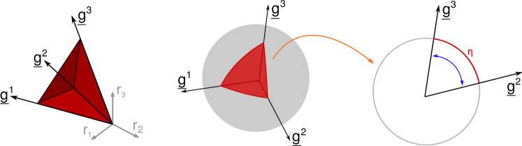
Supplementary Figure S15: Convex polyhedral cone and its section on a sphere. Left: the feasibility domain is a convex polyhedral cone, which is completely determined by its $S$ generators (when $S=3$ we have $3$ generators $\boldsymbol{g}^{1}$, $\boldsymbol{g}^{2}$, and $\boldsymbol{g}^{3}$). Center: since we consider a linear equation we can focus the analysis only on the intersection between the convex polyhedral cone and the unit sphere’s surface, which in three dimensions results in a spherical triangle. Right: each side of the convex polyhedral cone can be determined from a pair of generators as an arc $\eta$ of the sphere’s surface. Since we are considering the unit sphere, the arc length $\eta$ is equal to the angle between the two generators.

An important feature of convex polyhedral cones is that if $\boldsymbol{r}$ belongs to the cone, then so does $c\boldsymbol{r}$ for any positive constant $c$. As explained in section S3, this is a consequence of the linearity of equation S1. It is relevant therefore to limit our analysis to the growth rate vectors on the unit sphere, i.e., to vectors $\boldsymbol{r}$ such that

$$\|\boldsymbol{r}\|=\sqrt{r_{1}^{2}+r_{2}^{2}+r_{3}^{2}}=1\ .$$ (S126)

When we consider the vector in the feasibility domain on the surface of a unit sphere we obtain the areas of figure 1 in the main text. In this case, the quantity $\Xi$ is the area of the triangle, while the side lengths are the three sides of the triangle. Note that the polygon is not a triangle (as it lies on a sphere), but rather a spherical triangle. Its sides are arcs of a circumference, while its corners are identified by the three generators of the convex polyhedral cone.

In the $S=3$ case it is possible to obtain a closed expression for the area $\Xi$ Gourion2010 :

$$\Xi=\frac{8}{\pi}\arctan\Bigl{(}\frac{|\det(\boldsymbol{G})|}{1+\boldsymbol{g}^{1}\cdot\boldsymbol{g}^{2}+\boldsymbol{g}^{2}\cdot\boldsymbol{g}^{3}+\boldsymbol{g}^{1}\cdot\boldsymbol{g}^{3}}\Bigr{)}+\Theta\Bigl{(}-1-\boldsymbol{g}^{1}\cdot\boldsymbol{g}^{2}-\boldsymbol{g}^{2}\cdot\boldsymbol{g}^{3}-\boldsymbol{g}^{1}\cdot\boldsymbol{g}^{3}\Bigr{)}\ ,$$ (S127)

where the second term adds one to the first term when the argument of the arctangent is negative, while the matrix $\boldsymbol{G}$ is defined as

$$G_{ij}=\boldsymbol{g}^{i}\cdot\boldsymbol{g}^{j}\ .$$ (S128)

Equation S127 can be expressed directly in terms of the matrix $\boldsymbol{A}$ using equation S12.

S14  Nonlinear per capita growth rates

In general, the effect of a species on the per capita growth rate of other species is not linear. Equation S1 assumes this to be linear and the results presented in this paper were obtained under this assumption. Nonlinearity of the per capita growth rates can be thought of as a dependence of the interaction matrix $\boldsymbol{A}$ on $\boldsymbol{n}$:

$$\frac{\mathrm{d}n_{i}}{\mathrm{d}t}=n_{i}\left(r_{i}+\sum_{j=1}^{S}A_{ij}(\boldsymbol{n})n_{j}\right)\ .$$ (S129)

For instance, in the case of predator-prey interactions with a Holling type II functional response, it would have the form

$$A_{ij}(\boldsymbol{n})=\frac{A^{0}_{ij}}{1+\sum_{j}h_{ij}A^{0}_{ij}n_{j}}\ ,$$ (S130)

where the $h_{ij}$ are the handling times.

The presence of nonlinearity has strong consequences for both feasibility and stability. It is no longer possible to disentangle feasibility and stability with a simple condition on $A^{0}_{ij}$. This means that feasibility will depend not only on the direction of $\boldsymbol{r}$, but also on its length.

The results presented here are a necessary stepping stone for assessing the feasibility of nonlinear systems. When the degree of nonlinearity is small (e.g., $h_{ij}\approx 0$), one can use our results, valid for the case $h_{ij}=0$, to find the center of the feasibility domain and the generators. One can then treat the departure from $h_{ij}=0$ as a small perturbation, and therefore, instead of having to explore the full vast parameter space, use the solution of the linear case as a starting point for numerical calculations to converge on the actual, nonlinear feasibility domain. On the other hand, in the limit of very large $h_{ij}$ values, It is possible to show that the nonlinear form in equation S130 is approximately linear, and so again it is possible to use our method. The effect of intermediate values of $h_{ij}$ on the feasibility domain is, however, still an open question.

References

References

- [1] J F Gillooly, J H Brown, G B West, V M Savage, and E L Charnov. Effects of size and temperature on metabolic rate. Science (New York, N.Y.), 293(5538):2248–51, October 2001.
- [2] Gian-Reto Walther, Eric Post, Peter Convey, Annette Menzel, Camille Parmesan, Trevor J C Beebee, Jean-Marc Fromentin, Ove Hoegh-Guldberg, and Franz Bairlein. Ecological responses to recent climate change. Nature, 416(6879):389–95, March 2002.
- [3] Jason M. Tylianakis, Raphael K. Didham, Jordi Bascompte, and David A. Wardle. Global change and species interactions in terrestrial ecosystems. Ecology Letters, 11(12):1351–1363, December 2008.
- [4] Jason P Harmon, Nancy A Moran, and Anthony R Ives. Species response to environmental change: impacts of food web interactions and evolution. Science (New York, N.Y.), 323(5919):1347–50, March 2009.
- [5] Jason M. Tylianakis, Etienne Laliberté, Anders Nielsen, and Jordi Bascompte. Conservation of species interaction networks. Biological Conservation, 143(10):2270–2279, October 2010.
- [6] G. Meszéna, M. Gyllenberg, L. Pásztor, and J. A. J. Metz. Competitive exclusion and limiting similarity: a unified theory. Theoretical Population Biology, 69:68–87, 2006.
- [7] G. Barabás, L. Pásztor, G. Meszéna, and A. Ostling. Sensitivity analysis of coexistence in ecological communities: theory and application. Ecology Letters, 17:1479–1494, 2014.
- [8] György Barabás, Simone Pigolotti, Mats Gyllenberg, Ulf Dieckmann, and Géza Meszéna. Continuous coexistence or discrete species? A new review of an old question. Evolutionary Ecology Research, 14(5):523–554, 2012.
- [9] R. P. Rohr, S. Saavedra, and Jordi Bascompte. On the structural stability of mutualistic systems. Science, 345(6195):1253497–1253497, July 2014.
- [10] Robert M. May and Warren J. Leonard. Nonlinear Aspects of Competition Between Three Species. SIAM Journal on Applied Mathematics, 29(2):243–253, September 1975.
- [11] Robert M. May. Will a Large Complex System be Stable? Nature, 238(5364):413–414, August 1972.
- [12] Stefano Allesina and Si Tang. Stability criteria for complex ecosystems. Nature, February 2012.
- [13] Samir Suweis, Jacopo Grilli, and Amos Maritan. Disentangling the effect of hybrid interactions and of the constant effort hypothesis on ecological community stability. Oikos, 123(5):525–532, May 2014.
- [14] Stefano Allesina, Jacopo Grilli, György Barabás, Si Tang, Johnatan Aljadeff, and Amos Maritan. Predicting the stability of large structured food webs. Nature communications, 6:7842, January 2015.
- [15] R. H. MacArthur. Fluctuations of animal populations and a measure of community stability. Ecology, 36:533–536, 1955.
- [16] Michael E. Gilpin. Stability of feasible predator-prey systems. Nature, 254(5496):137–139, March 1975.
- [17] Alan Roberts. The stability of a feasible random ecosystem. Nature, 251(5476):607–608, October 1974.
- [18] B.S. Goh and L.S. Jennings. Feasibility and stability in randomly assembled Lotka-Volterra models. Ecological Modelling, 3(1):63–71, February 1977.
- [19] Serguei Saavedra, Rudolf P. Rohr, Jens M. Olesen, and Jordi Bascompte. Nested species interactions promote feasibility over stability during the assembly of a pollinator community. Ecology and Evolution, 6(4):997–1007, feb 2016.
- [20] Vito Volterra. Leçons sur la théorie mathématique de la lutte pour la vie. J. Gabay, 1931.
- [21] B. S. Goh. Global Stability in Many-Species Systems, 1977.
- [22] Dmitrii O. Logofet. Stronger-than-Lyapunov notions of matrix stability, or how “flowers” help solve problems in mathematical ecology. Linear Algebra and its Applications, 398:75–100, March 2005.
- [23] C. R. Johnson. Positive Definite Matrices. The American Mathematical Monthly, 77(3):259, mar 1970.
- [24] Si Tang and Stefano Allesina. Reactivity and stability of large ecosystems. Frontiers in Ecology and Evolution, 2:21, jun 2014.
- [25] Yu M. Svirezhev and Dmitriĭ Olegovich Logofet. The stability of biological communities. Nauka, Moscow, 1978.
- [26] Stefano Allesina and Si Tang. The stability–complexity relationship at age 40: a random matrix perspective. Population Ecology, 57(1):63–75, January 2015.
- [27] J E Cohen, F Briand, and C M Newman. Community food webs: Data and theory. Springer-Verlag, Berlin, 1990.
- [28] R J Williams and N D Martinez. Simple rules yield complex food webs. Nature, 404(6774):180–3, March 2000.
- [29] Jordi Bascompte, Pedro Jordano, Carlos J Melián, and Jens M Olesen. The nested assembly of plant-animal mutualistic networks. Proceedings of the National Academy of Sciences of the United States of America, 100(16):9383–7, August 2003.
- [30] Jordi Bascompte, Pedro Jordano, and Jens M Olesen. Asymmetric coevolutionary networks facilitate biodiversity maintenance. Science (New York, N.Y.), 312(5772):431–3, April 2006.
- [31] Ugo Bastolla, Miguel A Fortuna, Alberto Pascual-García, Antonio Ferrera, Bartolo Luque, and Jordi Bascompte. The architecture of mutualistic networks minimizes competition and increases biodiversity. Nature, 458(7241):1018–20, April 2009.
- [32] Elisa Thébault and Colin Fontaine. Stability of ecological communities and the architecture of mutualistic and trophic networks. Science (New York, N.Y.), 329(5993):853–6, August 2010.
- [33] R. Armstrong and R. McGehee. Coexistence of species competing for shared resources. Theoretical Population Biology, 9:317–328, 1976.
- [34] R. Armstrong and R. McGehee. Competitive exclusion. American Naturalist, 15:151–170, 1980.
- [35] P. A. Abrams. The theory of limiting similarity. Annual Review of Ecology and Systematics, 14:359–376, 1983.
- [36] P. Yodzis. The indeterminacy of ecological interactions as perceived through perturbation experiments. Ecology, 69:508–515, 1988.
- [37] J. M. Dambacher, H. W. Li, and P. A. Rossignol. Relevance of community structure in assessing indeterminacy of ecological predictions. Ecology, 83:1372–1385, 2002.
- [38] H. Aufderheide, L. Rudolf, T. Gross, and K. D. Lafferty. How to predict community responses to perturbations in the face of imperfect knowledge and network complexity. Proceedings of the Royal Society of London Series B, 280:20132355, 2013.
- [39] Samir Suweis, Filippo Simini, Jayanth R Banavar, and Amos Maritan. Emergence of structural and dynamical properties of ecological mutualistic networks. Nature, 500(7463):449–52, August 2013.
- [40] Alex James, Jonathan W Pitchford, and Michael J Plank. Disentangling nestedness from models of ecological complexity. Nature, 487(7406):227–30, July 2012.
- [41] G. Barabás and S. Allesina. Predicting global community properties from uncertain estimates of interaction strengths. Journal of the Royal Society Interface, 12:20150218, 2015.
- [42] Stefano Allesina and Mercedes Pascual. Food web models: a plea for groups. Ecology letters, 12(7):652–662, 2009.
- [43] Samir Suweis, Jacopo Grilli, Jayanth R Banavar, Stefano Allesina, and Amos Maritan. Effect of localization on the stability of mutualistic ecological networks. Nature communications, 6:10179, jan 2015.
- [44] Ray Redheffer. Volterra Multipliers II. SIAM Journal on Algebraic Discrete Methods, 6(4):612–623, oct 1985.
- [45] Jason M. Ribando. Measuring Solid Angles Beyond Dimension Three. Discrete & Computational Geometry, 36(3):479–487, oct 2006.
- [46] Daniel Gourion and Alberto Seeger. Deterministic and stochastic methods for computing volumetric moduli of convex cones. Computational & Applied Mathematics, 29(2):215–246, 2010.
- [47] Eugenius Kaszkurewicz and Amit Bhaya. Matrix Diagonal Stability in Systems and Computation. Birkhäuser Boston, Boston, MA, 2000.
- [48] Abraham Berman and Daniel Hershkowitz. Matrix diagonal stability and its implications. SIAM Journal on Algebraic Discrete Methods, 4(3):377–382, 1983.
- [49] R. Tyrrell Rockafellar. Convex Analysis. Princeton University Press, 1997.
- [50] Terence Tao, Van Vu, and Manjunath et al. Krishnapur. Random matrices: Universality of ESDs and the circular law. The Annals of Probability, 38(5):2023–2065, September 2010.
- [51] Terence Tao and Van Vu. Random Matrices: Universality of Local Eigenvalue Statistics up to the Edge. Communications in Mathematical Physics, 298(2):549–572, April 2010.
- [52] Terence Tao and Van Vu. Random matrices: Universality of local eigenvalue statistics. Acta Mathematica, 206(1):127–204, March 2011.
- [53] Stefano Allesina and Si Tang. The stability–complexity relationship at age 40: a random matrix perspective. Population Ecology, 57(1):63–75, jan 2015.
- [54] Giorgio Parisi. Statistical Field Theory. Perseus Books, 1998.
- [55] T. H. Berlin and M. Kac. The Spherical Model of a Ferromagnet. Physical Review, 86(6):821–835, June 1952.
- [56] Ted J. Case and Richard G. RG Casten. Global stability and multiple domains of attraction in ecological systems. The American Naturalist, 113(5):705–714, may 1979.
- [57] Jan O Haerter, Namiko Mitarai, and Kim Sneppen. Food Web Assembly Rules for Generalized Lotka-Volterra Equations. PLoS computational biology, 12(2):e1004727, feb 2016.
- [58] Joel E Cohen, Daniella N Schittler, David G Raffaelli, and Daniel C Reuman. Food webs are more than the sum of their tritrophic parts. Proceedings of the National Academy of Sciences, 106(52):22335–22340, 2009.
- [59] Robert R Christian and Joseph J Luczkovich. Organizing and understanding a winter’s seagrass foodweb network through effective trophic levels. Ecological Modelling, 117(1):99–124, 1999.
- [60] Marie-France Cattin Blandenier. Food web ecology: models and application to conservation. PhD thesis, 2004.
- [61] Edward B Baskerville, Andy P Dobson, Trevor Bedford, Stefano Allesina, T Michael Anderson, and Mercedes Pascual. Spatial guilds in the Serengeti food web revealed by a Bayesian group model. PLoS computational biology, 7(12):e1002321, 2011.
- [62] C Dieter Zander, Neri Josten, Kim C Detloff, Robert Poulin, John P McLaughlin, and David W Thieltges. Food web including metazoan parasites for a brackish shallow water ecosystem in Germany and Denmark: Ecological Archives E092-174. Ecology, 92(10):2007, 2011.
- [63] Kim N Mouritsen, Robert Poulin, John P McLaughlin, and David W Thieltges. Food web including metazoan parasites for an intertidal ecosystem in New Zealand: Ecological Archives E092-173. Ecology, 92(10):2006, 2011.
- [64] Neo D Martinez. Artifacts or attributes? Effects of resolution on the Little Rock Lake food web. Ecological Monographs, 61:367–392, 1991.
- [65] David W Thieltges, Karsten Reise, Kim N Mouritsen, John P McLaughlin, and Robert Poulin. Food web including metazoan parasites for a tidal basin in Germany and Denmark: Ecological Archives E092-172. Ecology, 92(10):2005, 2011.
- [66] Silvia Opitz. Trophic interactions in Caribbean coral reefs. Number 1085. WorldFish, 1996.
- [67] Ute Jacob, Aaron Thierry, Ulrich Brose, Wolf E Arntz, Sofia Berg, Thomas Brey, Ingo Fetzer, Tomas Jonsson, Katja Mintenbeck, Christian Mollmann, and Others. The role of body size in complex food webs: A cold case. Advances In Ecological Research, 45:181–223, 2011.
- [68] Ryan F Hechinger, Kevin D Lafferty, John P McLaughlin, Brian L Fredensborg, Todd C Huspeni, Julio Lorda, Parwant K Sandhu, Jenny C Shaw, Mark E Torchin, Kathleen L Whitney, and Others. Food webs including parasites, biomass, body sizes, and life stages for three California/Baja California estuaries: Ecological Archives E092-066. Ecology, 92(3):791, 2011.
- [69] Jens O Riede, Ulrich Brose, Bo Ebenman, Ute Jacob, Ross Thompson, Colin R Townsend, and Tomas Jonsson. Stepping in {E}lton’s footprints: a general scaling model for body masses and trophic levels across ecosystems. Ecology Letters, 14(2):169–178, 2011.
- [70] Ute Jacob. Trophic dynamics of Antarctic shelf ecosystems: food webs and energy flow budgets. PhD thesis, Bremen, Univ., Diss., 2005.
- [71] Serguei Saavedra, Rudolf P Rohr, Vasilis Dakos, and Jordi Bascompte. Estimating the tolerance of species to the effects of global environmental change. Nature communications, 4:2350, January 2013.