Uniformly Valid Confidence Sets Based on the Lasso

Abstract

In a linear regression model of fixed dimension $p\leq n$, we construct confidence regions for the unknown parameter vector based on the Lasso estimator that uniformly and exactly hold the prescribed in finite samples as well as in an asymptotic setup. We thereby quantify estimation uncertainty as well as the “post-model selection error” of this estimator. More concretely, in finite samples with Gaussian errors and asymptotically in the case where the Lasso estimator is tuned to perform conservative model selection, we derive exact formulas for computing the minimal coverage probability over the entire parameter space for a large class of shapes for the confidence sets, thus enabling the construction of valid confidence regions based on the Lasso estimator in these settings. The choice of shape for the confidence sets and comparison with the confidence ellipse based on the least-squares estimator is also discussed. Moreover, in the case where the Lasso estimator is tuned to enable consistent model selection, we give a simple confidence region with minimal coverage probability converging to one. Finally, we also treat the case of unknown error variance and present some ideas for extensions.

1 Introduction

The Lasso estimator as introduced in Tibshirani (1996) as well as many variants thereof have gained strong interest in the statistics community and in applied areas over the past two decades. As is well known, the main attraction of the Lasso estimator lies in its ability to perform model selection and parameter estimation at very low computational cost, see for instance Alliney & Ruzinsky (1994), Efron et al. (2004) and Rosset & Zhu (2007), and in the fact that the estimator can be used in high-dimensional settings where the number of variables $p$ exceeds the number of observations $n$ (“$p\gg n$”).

Recent years have seen an increased interest on how to perform valid inference in connection with these types of estimators. Pötscher & Schneider (2010) construct valid confidence intervals based on the Lasso as well as related estimators in the framework of linear regression models with orthogonal design and give an in-depth analysis of the problems and challenges that arise in this context. Generalizations of these results to a moderate-dimensional (orthogonal) setting where $p\leq n$ but $p$ diverging with $n$ can be found in Schneider (2016).

In a general high-dimensional setting with $p\gg n$, confidence regions and confidence intervals in connection with the Lasso estimator have recently been treated by different approaches. Based on Zhang & Zhang (2014), several papers including Van de Geer et al. (2014), Javanmard & Montanari (2014), Caner & Kock (2018) and Van de Geer & Stucky (2016) use the idea of “de-sparsifying” the Lasso estimator. In case where $p\leq n$ this approach essentially reduces to using the least-squares (LS) estimator for inference. In that sense this theory leaves a gap on how to construct confidence regions based on the Lasso estimator in a low-dimensional framework to provide uncertainty quantification for the Lasso estimator in this case.

Lee et al. (2016) consider finite-sample results for confidence intervals in connection with the Lasso estimator yet these authors take a different route in that their intervals are not set to cover the true parameter, but a pseudo-true value that depends on the selected model and coincides with the true parameter if the selected model is correct. All inference is conditional on the selected model. A model-dependent parameter is also covered in Berk et al. (2013) who discuss an intricate procedure for obtaining confidence regions for a pseudo-true parameter in connection with arbitrary model selection procedures.

In this paper, we construct confidence sets based on the Lasso estimator for the entire unknown parameter vector. We stress that while in the low-dimensional case the LS estimator can be employed to build confidence regions, the Lasso estimator is still used in such a framework, naturally entailing the question on how to conduct valid inference, and our results also quantify the worst-case estimation (“post-model selection”) error of this method. Moreover, Schneider & Ewald (2017) show that in high dimensions, the Lasso estimator may in fact act as a low-dimensional procedure in which case the results of this paper can also be applied.

One of the challenges of this task lies in the well-known fact that the finite-sample distribution of the Lasso estimator depends on the unknown parameter in a complicated manner. This phenomenon does not vanish for large samples as can be seen within a so-called moving-asymptotic framework (see Pötscher & Leeb (2009) for a detailed analysis in orthogonal design) and also occurs for related estimators. In order to construct valid confidence sets, we need to know the smallest coverage probability occurring over the whole parameter space. Pötscher & Schneider (2010) derive a formula for the minimal coverage probability of fixed-width confidence intervals based on the Lasso estimator in one dimension using knowledge of its finite-sample distribution. In the general case, this finite-sample distribution is not known, so it is not clear how to obtain an expression for the coverage probability in more than one dimension. Additionally, this coverage probability clearly depends on the shape that is used for the confidence set and it is a not clear a priori what this shape should be. We do the following.

While the finite sample distribution and therefore the coverage probability for any kind of set based on the Lasso estimator is unknown in general dimensions, we show that computing the minimal coverage probability can actually be carried out without this explicit knowledge. We obtain an explicit formula for the minimal coverage probability by, in a way, deferring the minimization problem into the objective function that defines the estimator, as is depicted in Section 3. For the confidence regions, we consider a large class of shapes that is determined by a condition involving the regressor matrix. This class encompasses the elliptic shape one would use if the confidence region was based on the LS estimator, thus enabling comparisons with the LS confidence ellipse. Analogously to the fixed-width intervals in Pötscher & Schneider (2010), the confidence regions we consider are random only through their centering at the Lasso estimator (which is also in line with the setup in the literature for high-dimensional settings, see for instance Van de Geer et al. 2014). Asymptotically, we distinguish between two regimes for the tuning parameters which we call conservative and consistent tuning. As suggested from the results in Pötscher & Schneider (2010), our results from finite samples essentially carry over asymptotically when the estimator is tuned conservatively. In the case of consistent tuning, the uniform convergence rate of the estimator is slower than $n^{-1/2}$ and we give the asymptotic distribution of the Lasso estimator when scaled by the appropriate factor corresponding to the uniform convergence rate, as well as suggesting a simple construction for a confidence set in that case.

The remaining paper is organized as follows. In Section 2 we set the framework by stating the model, defining the estimator and introducing some notation. The main result giving the formula for the minimal coverage probability is presented in Section 3 and subsequently Section 4 is devoted to discussing how to concretely construct the corresponding confidence sets, as well as their relationship to the confidence ellipse based on the LS estimator. We treat the case of unknown error variance in Section 5, as well as several ideas for extensions and further considerations. In Section 6 we derive asymptotic results both for the case of conservative and the case of consistent model selection. Section 7 concludes. All proofs are deferred to Appendix A.

Literature on distributional properties of the Lasso estimator in the low-dimensional setting ($p\leq n$) include the often-cited paper by Knight & Fu (2000) who derive the asymptotic distribution when the estimator is tuned to perform conservative model selection. Pötscher & Leeb (2009) give a detailed analysis in the framework of a linear regression model with orthogonal design and derive the distribution of the Lasso estimator in finite samples as well as in the two asymptotic regimes of consistent and conservative tuning. Implications of these results for confidence intervals are analyzed in Pötscher & Schneider (2010) and generalizations to a moderate-dimensional setting where $p\leq n$ but $p$ diverging with $n$ are contained in Pötscher & Schneider (2011) and Schneider (2016).

2 Setting and assumptions

Consider the linear model

$$y=X\beta+\varepsilon,$$

where $y$ is the observed $n\times 1$ data vector, X the $n\times p$ regressor matrix which is assumed to be non-stochastic with full column rank $p$, $\beta\in\mathbb{R}^{p}$ is the true parameter vector and $\varepsilon$ the unobserved error term defined on some probability space $(\Omega,\mathcal{A},P)$ and consisting of independent and identically distributed components with mean 0 and finite variance $\sigma^{2}$. We consider a componentwise tuned Lasso estimator $\hat{\beta}_{\text{\tiny L}}$, defined as the unique solution to the minimization problem

$$\min_{\upbeta\in\mathbb{R}^{p}}L_{n}(\upbeta)=\min_{\upbeta\in\mathbb{R}^{p}}\|y-X\upbeta\|^{2}+2\sum_{j=1}^{p}\lambda_{n,j}|\upbeta_{j}|,$$

where $\lambda_{n,j}$, are non-negative and non-random componentwise tuning parameters that allow to exclude parameters from penalization. Note that if $\lambda_{n,j}=0$ for all $j$, this estimator is equal to the ordinary least-squares (LS) estimator $\hat{\beta}_{\text{\tiny LS}}$ and that $\lambda_{n,j}=c>0$ for all $j$ corresponds to the “classical” Lasso estimator as proposed by Tibshirani (1996). For later use, let $\lambda_{n}=(\lambda_{n,1},\dots,\lambda_{n,p})^{\prime}$ and $\Lambda_{n}=\operatorname{diag}(\lambda_{n})$, the diagonal matrix whose diagonal elements are given by the components of $\lambda_{n}$. We use $\mathds{1}_{\{.\}}$ for the indicator function and make the following obvious definitions. For $a\in\mathbb{R}^{p}$ and $B\subseteq\mathbb{R}^{p}$, the set $a+B=B+a\subseteq\mathbb{R}^{p}$ is defined as the set $\{a+b:b\in B\}$. For a $p\times p$ matrix $\bar{C}$ and a scalar $c$, the sets $\bar{C}B$ and $cB$ in $\mathbb{R}^{p}$ are $\{\bar{C}b:b\in B\}\subseteq\mathbb{R}^{p}$ and $\{cb:b\in B\}\subseteq\mathbb{R}^{p}$, respectively. Finally, for $k\in\mathbb{N}$, $I_{k}$ stands for the $k\times k$ identity matrix and $\overline{\mathbb{R}}$ denotes the extended real line $\mathbb{R}\cup\{-\infty,\infty\}$.

3 Finite-sample results

We aim to construct confidence sets for the entire parameter vector $\beta$ based on the Lasso estimator $\hat{\beta}_{\text{\tiny L}}$. That means that for a non-random set $M\subseteq\mathbb{R}^{p}$, we consider sets of the form

$$\hat{\beta}_{\text{\tiny L}}-M=\{\hat{\beta}_{\text{\tiny L}}-m:m\in M\},$$

which have to satisfy that the probability of actually covering the unknown parameter $\beta$ never (for no value of $\beta$) falls below a prescribed level $1-\alpha$ with $\alpha\in[0,1]$. In other words, we need $P_{\beta}(\beta\in\hat{\beta}_{\text{\tiny L}}-M)\geq 1-\alpha$ for all $\beta\in\mathbb{R}^{p}$ (where we stress the dependence of the probability measure on $\beta$ whenever it occurs), so that

$$\inf_{\beta\in\mathbb{R}^{p}}P_{\beta}(\beta\in\hat{\beta}_{\text{\tiny L}}-M)\geq 1-\alpha.$$

In order to achieve this, we need to be able to compute this “infimal” (minimal) coverage probability. Throughout this and the two subsequent sections we suppose that the errors as normally distributed

$$\varepsilon\sim N(0,\sigma^{2}I_{n}),$$

although our results do not heavily depend on this assumption, also see Remark 1. The assumption that will be removed for asymptotic results in Section 6. We will show that the minimum occurs when the components of the unknown parameter become large in absolute value by essentially doing the following. We reparametrize the objective function defining the Lasso estimator so that the dependence on the unknown parameter becomes more transparent and easier to handle. We then consider the limiting cases of the objective functions when the components of the unknown parameter vector $\beta$ become large in absolute value (that is, tend to $+\infty$ or $-\infty$). We will see that it is possible to minimize the resulting objective functions explicitly, with minimizers that follow a shifted normal distribution that has the same covariance matrix as the LS estimator and by construction do not depend on the unknown parameter. Finally, we will show that the infimal coverage probability of the proposed sets is indeed “achieved” for one of these finitely many limiting cases.

To state the main theorem, we need several definitions. First we define the reparametrized objective function $Q_{n}(u)=L_{n}(\beta+n^{-1/2}u)-L_{n}(\beta)$ so that $Q_{n}$ is uniquely minimized at $\hat{u}_{n}=n^{1/2}(\hat{\beta}_{\text{\tiny L}}-\beta)$, the estimation error scaled by $n^{1/2}$. Of course, this scaling factor is arbitrary in finite samples, but proves to be of advantage when considering the problem in large samples in Section 6.1. We can write $Q_{n}$ as

$$Q_{n}(u)=u^{\prime}C_{n}u-2u^{\prime}W_{n}+2n^{-1/2}\sum_{j=1}^{p}\lambda_{n,j}\left[|u_{j}+n^{1/2}\beta_{j}|-|n^{1/2}\beta_{j}|\right],$$

where $C_{n}=X^{\prime}X/n$ and $W_{n}=n^{-1/2}X^{\prime}\varepsilon\sim N(0,\sigma^{2}C_{n})$. Note that for a set $M\subseteq\mathbb{R}^{p}$ we then have

$$P_{\beta}(\beta\in\hat{\beta}_{\text{\tiny L}}-n^{-1/2}M)=P_{\beta}(\hat{u}_{n}\in M).$$

The above mentioned limiting cases of the objective function that we consider are defined as

$$Q_{n}^{d}(u)=u^{\prime}C_{n}u-2u^{\prime}W_{n}+2n^{-1/2}\sum_{j=1}^{p}\lambda_{n,j}d_{j}u_{j},$$ (1)

where $d=(d_{1},\dots,d_{p})^{\prime}\in\{-1,1\}^{p}$. Holding $W_{n}$ fixed for a moment, we indeed see that

$$Q^{d}_{n}(u)=\lim_{d_{j}\beta_{j}\to\infty\atop j=1,\dots,p}Q_{n}(u).$$

As shorthand notation, we write $\hat{u}_{n}^{d}$ for the unique minimizer of $Q_{n}^{d}$. To define the shape that we want to consider for the confidence regions, we introduce the following notation. For $m\in\mathbb{R}^{p}$, a vector $d\in\{-1,1\}^{p}$ and a matrix $\bar{C}\in\mathbb{R}^{p\times p}$, we define

$$A_{\bar{C}}^{d}(m)=\bigcap_{j=1}^{p}\{z\in\mathbb{R}^{p}:d_{j}(\bar{C}m)_{j}\leq d_{j}(\bar{C}z)_{j},d_{j}z_{j}\leq 0\}.$$

The set $A_{\bar{C}}^{d}(m)$ is an intersection of $2p$ half-spaces, $p$ of which determine the orthant the set is located in via the parameter $d$. The other $p$ half-spaces are defined by hyperplanes that intersect at the point $m$. Figure 1 shows one example of such a set. Note that in general, $A_{\bar{C}}^{d}(m)$ could be non-empty also for $\operatorname{sgn}(m)\neq-d$.

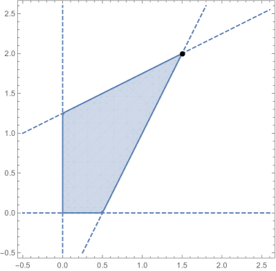
Figure 1: The set $A_{\bar{C}}^{-\iota}(m)$ with $\iota=(1,1)^{\prime}$, $m=(1.5,2)^{\prime}$ and $\bar{C}=\left(\begin{smallmatrix}1&-0.5\\ -0.5&1\end{smallmatrix}\right)$ along with the hyperplanes defining the set. The point $m=(1.5,2)^{\prime}$ is displayed as a dot.

The sets we consider are determined by the following condition.

Condition A.

Let $\bar{C}\in\mathbb{R}^{p\times p}$ be given. We say that a set $M\subseteq\mathbb{R}^{p}$ satisfies Condition A with matrix $\bar{C}$ if

$$A_{\bar{C}}^{d}(m)\subseteq M$$

for all $d\in\{-1,1\}^{p}$ and for all $m\in M$.

The above condition will be discussed in more detail in Section 4. Using this notation, we can now state the main theorem.

Theorem 1.

If $M_{n}\subseteq\mathbb{R}^{p}$ is non-random and satisfies Condition A with $\bar{C}=C_{n}$, then

$$\inf_{\beta\in\mathbb{R}^{p}}P_{\beta}(\hat{u}_{n}\in M_{n})=\min_{d\in\{-1,1\}^{p}}P(\hat{u}_{n}^{d}\in M_{n}),$$

where $\hat{u}_{n}^{d}\sim N(-n^{-1/2}C_{n}^{-1}\Lambda_{n}d,\sigma^{2}C_{n}^{-1})$.

The distributions of $\hat{u}^{d}_{n}$ determining the formula for the infimal coverage probability are shifted normal distributions with the same covariance matrix as the corresponding (shifted and scaled) LS estimator $\hat{u}_{\text{\tiny LS}}=n^{1/2}(\hat{\beta}_{\text{\tiny LS}}-\beta)$ and mean that depends on the regressors and the vector of tuning parameters.

Remark 1.

Note that (the proof of) Theorem 1 does not hinge on the normality assumption, as it exploits the structure of the underlying optimization problem rather than stochastic properties of the error distribution. Different error distributions could be used in Theorem 1, only the distributions of $\hat{u}_{n}^{d}$ would have to be adapted accordingly.

Since Condition A for $p=1$ simply requires the corresponding set $M_{n}$ to be an interval containing zero, Theorem 1 is indeed a generalization of the formula in Theorem 5(a) in Pötscher & Schneider (2010), as discussed in the introduction. (To make the connection, note that the tuning parameter $\eta_{n}$ in that reference corresponds to a component $n^{-1/2}\lambda_{n,j}$ of the vector of tuning parameters in our paper.) The following obvious corollary specifies the resulting valid confidence region based on the Lasso estimator.

Corollary 2.

Let $0<\alpha<1$. If $M_{n}\subseteq\mathbb{R}^{p}$ is non-random and satisfies Condition A with $\bar{C}=C_{n}$, as well as $\min_{d\in\{-1,1\}^{p}}P(\hat{u}_{n}^{d}\in M_{n})=1-\alpha$ with $\hat{u}_{n}^{d}\sim N(-n^{-1/2}C_{n}^{-1}\Lambda_{n}d,\sigma^{2}C_{n}^{-1})$, then

$$\inf_{\beta\in\mathbb{R}^{p}}P_{\beta}(\beta\in\hat{\beta}_{\text{\tiny L}}-n^{-1/2}M_{n})=1-\alpha.$$

4 Constructing the confidence set

We now turn to discussing the important matter of how to choose an appropriate set $M_{n}\subseteq\mathbb{R}^{p}$ for some desired level of confidence $1-\alpha$ by discussing concrete shapes for the confidence regions as well as their size and relation to confidence sets based on the LS estimator. As mentioned in the previous section, we need to find a set $M_{n}\subseteq\mathbb{R}^{p}$ that satisfies Condition A with $\bar{C}=C_{n}$ and such that $\min_{d\in\{-1,1\}^{p}}P(\hat{u}_{n}^{d}\in M_{n})=1-\alpha$ where

$$\hat{u}_{n}^{d}\sim N(-n^{-1/2}C_{n}^{-1}\Lambda_{n}d,\sigma^{2}C_{n}^{-1}).$$

The resulting confidence set for $\beta$ is then the scaled and shifted set $\hat{\beta}_{\text{\tiny L}}-M_{n}/n^{1/2}$. If we would base the set on the LS estimator $\hat{\beta}_{\text{\tiny LS}}$ instead of $\hat{\beta}_{\text{\tiny L}}$, the canonical and best choice for $M_{n}$ in terms of volume is an ellipse determined by the contour lines of a $N(0,\sigma^{2}C_{n}^{-1})$-distribution, the $C_{n}$-ellipse. Given the fact that the covariance matrix of the distributions of $\hat{u}^{d}_{n}$ is in fact $\sigma^{2}C_{n}^{-1}$, in addition to the fact that the means of the distributions average to 0, it is reasonable to consider the $C_{n}$-ellipse as a shape in connection with the Lasso estimator also. As stated in the following proposition, this shape complies with Condition A.

Proposition 3.

The $C_{n}$-ellipse given by

$$E_{C_{n}}(k)=\{z\in\mathbb{R}^{p}:z^{\prime}C_{n}z\leq k\}$$

satisfies Condition A with $\bar{C}=C_{n}$ for any $k>0$.

How to choose the parameter $k$ for a given level of coverage $1-\alpha$ is stated in the next proposition.

Proposition 4.

For any $k>0$, we have that

$$\operatorname*{\arg\min}_{d\in\{-1,1\}^{p}}P\left(\hat{u}_{n}^{d}\in E_{C_{n}}(k)\right)=\operatorname*{\arg\max}_{d\in\{-1,1\}^{p}}\|C_{n}^{-1/2}\Lambda_{n}d\|.$$

Note that if $d^{*}$ solves the above optimization problem, so does $-d^{*}$. To finally obtain the confidence ellipse based on the Lasso estimator, pick any such optimizer $d^{*}$ and compute $k^{*}>0$ so that $P(u_{n}^{d^{*}}\in E_{C_{n}}(k^{*}))=1-\alpha$, which is easily done based on the following proposition.

Proposition 5.

For $0<\alpha<1$ we have $P(\hat{u}_{n}^{d}\in E_{C_{n}}(\sigma^{2}\kappa))=1-\alpha$ for

$$\kappa=(\chi^{2}_{p,\nu})^{-1}(1-\alpha),$$

where $(\chi^{2}_{p,\nu})^{-1}$ is the quantile function of a non-central $\chi^{2}$-distribution with $p$ degrees of freedom and non-centrality parameter

$$\nu=\frac{1}{n\sigma^{2}}d^{\prime}\Lambda_{n}C_{n}^{-1}\Lambda_{n}d.$$

Note that Proposition 5 also shows that the ellipse $E_{C_{n}}(k^{*})$, and therefore the resulting confidence set based on the Lasso estimator, is larger in volume than the one based on the LS estimator, since $P(\beta\in\hat{\beta}_{\text{\tiny LS}}-E_{C_{n}}(\sigma^{2}\kappa))=1-\alpha$ is satisfied for $\kappa=(\chi^{2}_{p})^{-1}(1-\alpha)$ where $(\chi^{2}_{p})^{-1}$ is the quantile function of a (central) $\chi^{2}$-distribution with $p$ degrees of freedom. Clearly, the difference in size will increase as the tuning parameters become large as then the non-centrality parameter $\nu$ will grow. These observations are in line with the findings in Pötscher & Schneider (2010) who show that a confidence interval based on the Lasso estimator is larger than a confidence interval based on the LS estimator with the same coverage probability.

When comparing the two confidence sets, we emphasize that since the ellipses are centered at different values, the smaller ellipse based on the LS estimator is in general not contained in the ellipse based on the Lasso estimator. This, as well as the difference in volume between the two ellipses, will also be illustrated in the example below.

It is quite obvious that the $C_{n}$-ellipse is not optimal as a shape for confidence sets based on the Lasso estimator since we can get higher coverage with a set of the same volume by adjusting the ellipse “towards” the contour lines of the $N(-n^{-1/2}C_{n}^{-1}\Lambda_{n}d^{*},\sigma^{2}C_{n}^{-1})$-distributions (in such a way that Condition A is preserved). To find the best shape possible, one would have to minimize the volume of the set over all possible shapes satisfying Condition A subject to the constraint of holding the prescribed minimal coverage probability. This is a highly complex optimization problem and we do not dwell further on this subject here, but illustrate possible ways to construct “good” sets, as shown in the example below. Before discussing this further, note that the following proposition shows that it is easy to find the closure of an arbitrary subset of $\mathbb{R}^{p}$ with respect to Condition A.

Proposition 6.

For any $M\subseteq\mathbb{R}^{p}$, the set

$$\bigcup_{m\in M}\bigcup_{d\in\{-1,1\}^{p}}A^{d}_{\bar{C}}(m)$$

is the smallest set containing $M$ that satisfies Condition A.

We now provide an example for $p=2$ illustrating the difference between the confidence ellipse based on the LS estimator and the one based on the Lasso, as well as how to choose a better shape in terms of volume for the confidence set based on the Lasso estimator. The simulations and calculations were carried out using the statistical software package R. The example is set up in the following way. We let $n=20$ and generate the $(n\times 2)$-matrix $X$ using independent and identically distributed standard normal entries that are transformed row-wise by an appropriate $(2\times 2)$-matrix in order to get

$$C_{n}=\frac{X^{\prime}X}{n}=\begin{pmatrix}1&-0.5\\ -0.5&1\end{pmatrix}.$$

We generate the data vector $y$ from the corresponding linear model with $\sigma^{2}=1$ (so that $\varepsilon\sim N(0,I_{n})$) and true parameter chosen as $\beta=(1,0)^{\prime}$. We compute the Lasso estimator using the glmnet-package and tuning parameters $\lambda_{n,1}=\lambda_{n,2}=\sqrt{n}/2$ (asymptotically corresponding to what we will refer to as conservative model selection in the subsequent section). We also considered estimators where the tuning parameters were chosen by 10-fold cross-validation (as provided in the glmnet-package) which ended up yielding comparable results for the estimator.

We then constructed confidence ellipses with level $\alpha=0.05$ based on both the LS and the Lasso estimator in the manner described earlier in this section. The resulting sets are shown in Figure 2.

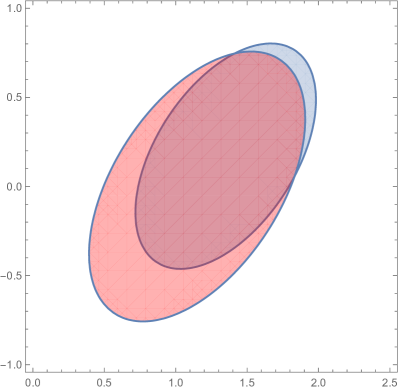
Figure 2: The confidence ellipses based on and centered at the Lasso estimator $\hat{\beta}_{\text{\tiny L}}=(1.15,0)^{\prime}$ (red) and the smaller one based on and centered at the LS estimator $\hat{\beta}_{\text{\tiny LS}}=(1.35,0.17)^{\prime}$ (blue), respectively.

The plot clearly illustrates the above described fact that the confidence ellipse based on the Lasso estimator is larger than the confidence ellipse that is based on the LS estimator. Also, the two sets are overlapping by a large amount (in fact, the maximal distance between the two estimators is controlled by Proposition 16 in the Appendix). However, the LS ellipse is not entirely contained in the one based on the Lasso, stressing the fact the Theorem 1 yields non-trivial sets.

The above comparison between the two ellipses, however, is somewhat unfair in the sense that the shape used for both confidence sets is the optimal one (in terms of volume) for the LS estimator, but, as discussed above, not for the Lasso estimator. With the optimal shape for a Lasso confidence set being unknown, we at least want to find a shape that improves upon the ellipse. As a basis for this, we consider the union of the contour sets corresponding to the distributions of $\hat{u}_{n}^{d}$, that is, the $2^{p}$ shifted $C_{n}$-ellipses

$$U_{n}(k)\;=\bigcup_{d\in\{-1,1\}^{p}}E_{C_{n}}(k)-n^{-1/2}C_{n}^{-1}\Lambda_{n}d,$$

where each set in the union is of optimal shape for the corresponding distribution of $\hat{u}_{n}^{d}$. As a starting point, we choose $k$ so that $P(\hat{u}_{n}^{d}\in E_{C_{n}}(k)-n^{-1/2}C_{n}^{-1}\Lambda_{n}d)=1-\alpha$ (note that $k$ is then simply the parameter of the $C_{n}$-ellipse used for the LS estimator, but any $k>0$ such that $U_{n}(k)$ satisfies $P(\hat{u}_{n}^{d}\in U_{n}(k))\geq 1-\alpha$ works). Clearly, this set is still too large and will not satisfy Condition A, so we need to address these two issues. First, we add all points necessary so that the resulting set satisfies Condition A. Proposition 6 ensures that

$$\bigcup_{m\in U_{k}}\bigcup_{d\in\{-1,1\}^{p}}A_{C_{n}}^{d}(m)$$

fulfills the desired condition. Note that in this particular case, it is fairly straightforward to see that this set is simply given by the convex hull of the shifted ellipses $U_{n}(k)$. Finally, to get the smallest set with this shape that still holds the prescribed level of coverage, we iteratively adjust the set by reducing the parameter $k$ and re-calculate the minimal coverage probability of the resulting set until the desired minimal coverage probability is reached (up to an arbitrary level of precision). The resulting alternatively shaped set is depicted in Figure 3, LABEL:sub@subfig:construct showing the midpoints of the $2^{p}=4$ ellipses used in the construction and LABEL:sub@subfig:improved displaying the new confidence set on top of the elliptic confidence region based on the Lasso as devised before. It is obvious that the new shape has slightly less volume than the ellipse.

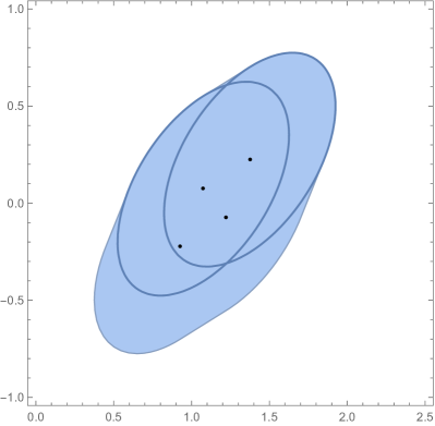
(a)

(b)

Figure 3: LABEL:sub@subfig:construct Construction of the alternative shape based on $2^{p}=4$ ellipses with their centers displayed as dots. LABEL:sub@subfig:improved The resulting improved confidence set with the alternative shape (blue) and the previous elliptic shape (red), both based on at the Lasso estimator $\hat{\beta}_{\text{\tiny L}}=(1.15,0)^{\prime}$.

5 Extensions and further considerations

In Section 5.1 we extend the previous results for the case of unknown error variance. Furthermore, we provide some insights on how the coverage probability of Lasso confidence regions might vary over the parameter space in Section 5.2 and illustrate some ideas on how to build confidence intervals for a single component of the parameter vector in Section 5.2, the latter two sections considering for the simple case of $p=2$.

5.1 Unknown error variance

As the results in Section 4 on how to construct the confidence regions use knowledge of the error variance $\sigma^{2}$. We now turn to the more realistic setting when the error variance is unknown and extend our findings to this framework. Let

$$\hat{\sigma}^{2}=\frac{1}{n-k}\hat{\varepsilon}_{\text{\tiny LS}}^{\prime}\hat{\varepsilon}_{\text{\tiny LS}},$$

the usual unbiased estimator of $\sigma^{2}$ based on the LS residuals $\hat{\varepsilon}_{\text{\tiny LS}}=y-X\hat{\beta}_{\text{\tiny LS}}$.

To apply the previous results to this setting, we let the tuning parameter $\lambda$ depend on the variance estimate in the following way. For this subsection, set $\lambda_{n}=\gamma_{n}/\hat{\sigma}$, where $\gamma_{n}\in\mathbb{R}^{p}$ with $\gamma_{n,j}\geq 0$ let $\hat{u}_{n}^{d}$ be defined as before. Since the main argument for proving the results leading up to Corollary 2 depend on the minimization problem rather than on stochastic properties, inspection of the corresponding proofs reveals that the minimal coverage probability can still be computed correspondingly. Not too surprisingly, rather than using (non-central) normal distributions, we need to consider (non-central) $t$-distributions when the variance is estimated. We summarize this in the following corollary.

Corollary 7.

For $\lambda_{n}=\gamma_{n}/\hat{\sigma}$ and if $M_{n}\subseteq\mathbb{R}^{p}$ is non-random and satisfies Condition A, we have that

$$\inf_{\beta\in\mathbb{R}^{p}}P_{\beta}(\beta\in\hat{\beta}_{\text{\tiny L}}-\hat{\sigma}M_{n})=\min_{d\in\{-1,1\}^{p}}P(\hat{u}_{n}^{d}\in\hat{\sigma}M_{n})=\min_{d\in\{-1,1\}^{p}}P(\hat{t}_{n}^{d}\in M_{n}),$$

where $\hat{t}_{n}^{d}\sim T(n-p,-n^{-1/2}C_{n}^{-1}\Gamma_{n}d,C_{n}^{-1})$ is a multivariate non-central $t$ distribution with $n-p$ degrees of freedom, non-centrality parameter $\mu=-n^{-1/2}C_{n}^{-1}L_{n}d$ where $\Gamma_{n}=\operatorname{diag}(\gamma_{n})$, and matrix $C_{n}^{-1}$.

One can now construct confidence regions in case where $\sigma^{2}$ is unknown. Note that the shape of the contour sets of the above $t$-distribution is the same as for the original distribution of $\hat{u}_{n}$, namely $E_{C_{n}}(k)=\{z\in\mathbb{R}^{p}:z^{\prime}C_{n}z\leq k\}$. Therefore, all considerations from Section 4 also apply in this setting, only the choice of the parameter $k$ needs to be adapted.

5.2 Coverage probabilities over the parameter space

Since the derivation of Theorem 1 intimates that the minimal coverage probability occurs for “large” values of the unknown parameter one might ask how the coverage looks for “small” values. As explicit expressions for the coverage probability are not known, we give plots of the simulated coverage probability of the 95% Lasso ellipse for $p=2$ for positive and negative correlation of the two components in Figure 4.

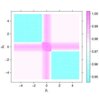
(a)

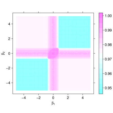
(b)

  

Figure 4: The coverage probability of the Lasso ellipse for $p=2$, $1\!-\!\alpha=0.95$, $n=20$ and LABEL:sub@subfig:coverage1 $C_{n}=\left(\begin{smallmatrix}1&0.5\\ 0.5&1\end{smallmatrix}\right)$ and LABEL:sub@subfig:coverage2 $C_{n}=\left(\begin{smallmatrix}1&-0.5\\ -0.5&1\end{smallmatrix}\right)$.

As can be seen, the minimal coverage occurs when the true parameter is “not small”. More concretely, for the case of positive correlation it occurs when both components are of opposite signs, and in case of negative correlation it occurs when both components are of the same sign. It can also be seen that in case the parameter space is known to be sparse (for $p=2$, this means that at least one component of the parameter vector is equal to 0), the minimal coverage over the restricted parameter space will certainly be higher than the minimal coverage over the entire parameter space. We cannot provide analytic expressions for minimal coverage probability over a sparse parameter space using our theory and it covers the case where no additional information about the parameter space is available. It can, however, also be gleaned from Figure 4 that the common restriction of assuming that the true parameter is either equal to zero or bounded away from zero (asymptotically at a certain rate) does not alleviate the situation for the Lasso estimator!

5.3 Inference on single components

We now consider the case where one might be interested in covering only a subvector of the entire unknown parameter vector. While it is clear that projecting the confidence region constructed for the entire parameter vector to the appropriate subspace will yield a valid confidence set for this purpose, it will generally not result in the most favorable shape.

In this subsection, we assume that the goal is to cover a single component of the parameter vector and give general considerations on how to determine the shape of the confidence region for the entire parameter vector so that the projection onto the single component of interest will yield the smallest symmetric interval possible.

More formally, consider the following. Assume that we want to construct a confidence interval for $\beta_{j}$, the $j$-th component of the unknown parameter vector $\beta$, with level of coverage $1-\alpha$. For this, we want to choose $M\subseteq\mathbb{R}^{p}$ such that

• $M$ satisfies Condition A.

• $\sup_{m\in M}|m_{j}|=a<\infty$.

• $\inf_{d\in\{-1,1\}^{p}}P(\hat{u}_{n}^{d}\in M)=1-\alpha$.

Clearly, this can be achieved by finding for any fixed but arbitrary $a\geq 0$ the largest set that satisfies Condition A and then choosing $a$ so that the prescribed coverage level is achieved. Note that this set may be unbounded with respect to the components that are not of interest. We construct the optimal shape for this explicitly for the case where $p=2$, assuming that both components are penalized (both $\lambda_{1}$ and $\lambda_{2}$ are non-zero) in the following section.

Constructing the optimal shape in case $p=2$

The following construction yields the set $M$ as described above for the case of $p=2$. Without loss of generality, we assume that we are interested in covering $\beta_{1}$, the first component of $\beta$. Recall that $C_{n}=X^{\prime}X/n$. If $C_{n}$ is diagonal, it is easily seen that the set

$$\tilde{M}=\{z\in\mathbb{R}^{2}:|z_{1}|\leq a\}$$

complies with Condition A and cannot be enlarged while maintaining a fixed projection onto the subspace associated with the first component. Also note that in this case, the resulting confidence interval will coincide with the one suggested in Pötscher & Schneider (2010).

If $C_{n}$ is not diagonal, assume that the off-diagonal element $c_{12}$ satisfies $c_{12}>0$. Define

$$M=\bigcup_{d\in\{-1,1\}^{2}}M^{d}$$

with

$$M^{(1,1)}=\tilde{M}\cap\{z\in\mathbb{R}^{2}:z_{1},z_{2}\geq 0,(C_{n}z)_{1}\leq(C_{n}\underline{a})_{1}\},$$

where $\underline{a}=(a,0)^{\prime}$ and

$$M^{(-1,1)}=\tilde{M}\cap\{z\in\mathbb{R}^{2}:z_{1}\leq 0,z_{2}\geq 0,(C_{n}z)_{2}\leq(C_{n}\underline{b})_{2}\},$$

where $\underline{b}=(0,b)^{\prime}$ satisfies $(C_{n}\underline{a})_{1}=(C_{n}\underline{b})_{1}$. Moreover, we define

$$M^{(-1,-1)}=-M^{(1,1)}\;\;\text{ and }\;\;M^{(1,-1)}=-M^{(-1,1)}.$$

The shape of the resulting set is depicted in Figure 5.

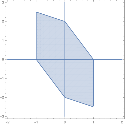
Figure 5: The set $\mathcal{M}$ for $C=\left(\begin{smallmatrix}1&0.5\\ 0.5&1\end{smallmatrix}\right)$ and $a=1$.

Note that, even though we are only interested in a confidence set that is bounded for one of the components, the need to comply with Condition A forces us to bound the set in the other component as well whenever $c_{12}\neq 0$. The interpretation of this fact is the following. As the Lasso can be viewed as a shifted LS estimator where the size and direction of the shift depend on both components of the LS estimator, we need to ensure that the influence of the second parameter on the shift is also corrected for by the procedure.

The following proposition ensures that $M$ satisfies Condition A and does indeed yield the largest such set with fixed projection $[-a,a]$ onto the first component – therefore providing the shape that results in the smallest confidence interval for $\beta_{1}$.

Proposition 8.

The set $M\subseteq\mathbb{R}^{2}$ as defined above satisfies Condition A. Moreover, if another $\bar{M}\subseteq\mathbb{R}^{2}$ with $\max_{m\in\bar{M}}|m_{1}|\leq a$ satisfies Condition A also, $\bar{M}\subseteq M$ follows.

It is again easily seen that for a given coverage probability $1-\alpha$, the quantity $a$ must be greater than the half-length of the standard interval based on the LS estimator, that is, the $(1-\alpha/2)$-quantile of the standard normal distribution. One might now be interested in the size difference between the confidence intervals constructed from the Lasso and LS estimates, respectively. Pötscher & Schneider (2010) have already shown that in the orthogonal regressor case, the length of confidence intervals which are based on the Lasso is greater than the length of the standard interval and that the difference increases with the penalization parameter $\lambda_{n}=(\lambda_{n,1},\lambda_{n,2})^{\prime}$. Table 1 contains the required values of $a$, that is, the half-lengths of the Lasso confidence interval for $c_{11}=c_{22}=1$, $\sigma^{2}=1$ and various combinations of $\bar{\lambda}=\lambda_{n,1}=\lambda_{n,2}$ and $c_{12}$. Note that in this case the LS estimator is the the Lasso estimator with $\bar{\lambda}=0$.

$|c_{12}|$	0.25	0.5	0.75	0.9
$\bar{\lambda}=0$	1.96	1.96	1.96	1.96
$\bar{\lambda}=0.1$	2.1	2.4	3.1	4.9
$\bar{\lambda}=0.5$	2.4	2.9	4.5	8.8
$\bar{\lambda}=1$	3.0	3.9	6.5	13.8
$\bar{\lambda}=2$	4.4	5.9	10.5	23.8
$\bar{\lambda}=3$	5.7	7.9	14.5	33.8

Table 1: Half-lengths of the 95% confidence intervals based on an equally tuned Lasso estimator for and $c_{11}=c_{22}=1$ and $\sigma^{2}=1$.

For small values of $\bar{\lambda}$ and $c_{12}$, the resulting confidence interval is only slightly longer than the one based on the LS estimator. For increasing $\bar{\lambda}$ and $|c_{12}|$, the required length of the interval increases significantly, in particular in the latter case, with the length more than doubling as $c_{12}$ increases from 0.25 to 0.9 for each of the presented values of $\bar{\lambda}>0$. This ratio is even more extreme for larger values of $\bar{\lambda}>0$. Two effects are at play here. On the one hand, the area of $M$ decreases for fixed $a>0$ as $c_{12}$ increases. On the other hand, some of the corners of the distorted $\lambda$-box, $-n^{-1/2}C_{n}^{-1}\Lambda_{n}d$ with $d\in\{−1,1\}^{p}$, which are the means of the normal distributions that must be covered, shift further apart as $c_{12}$ increases in absolute value. Obviously, increasing the tuning parameter also shifts the means further away from the origin, resulting in even larger confidence sets.

6 Asymptotic framework

We now derive asymptotic results that hold without assuming normality of the errors. Additionally to the assumptions in Section 2, for all asymptotic considerations, we assume that $X=(x_{1}^{\prime},\dots,x_{n}^{\prime})^{\prime}$ where $x_{i}^{\prime}\in\mathbb{R}^{p}$, meaning that the regressor matrix $X$ changes with $n$ only by appending rows, and that

$$C_{n}=\frac{X^{\prime}X}{n}\longrightarrow C$$

as $n\to\infty$, where $C$ is finite and positive definite. This setting assures consistency and asymptotic normality of the LS estimator. We will consider two different regimes of the asymptotic behavior of the tuning parameter $\lambda_{n}$ and start with the regime we call conservative tuning.

6.1 Conservative tuning

In this regime and throughout this subsection, we require that

$$\frac{\lambda_{n}}{n^{1/2}}\longrightarrow\lambda\in[0,\infty)^{p}$$

as $n\to\infty$. This implies that $\lambda_{n,j}/n\to 0$ for all $j=1,\dots,p$ , which in turn implies consistency of $\hat{\beta}_{\text{\tiny L}}$ (see Theorem 1 in Knight & Fu (2000) with the slight modification that in our paper we allow for componentwise defined tuning parameters). We let $\Lambda=\operatorname{diag}(\lambda)$.

Remark 2.

Such a choice of tuning parameters indeed yields a conservative model selection procedure in the sense that

$$\limsup_{n\to\infty}\sup_{\beta\in\mathbb{R}^{p}}P_{\beta}\left(\hat{\beta}_{j}=0\right)<1$$ (2)

for each $j=1,\dots,p$. In particular, if $\beta_{j}=0$, we have

$$\limsup_{n\to\infty}P_{\beta}\left(\hat{\beta}_{j}=0\right)<1.$$

The latter statement was also noted by Zou (2006) in Proposition 1.

The following proposition implicitly states the asymptotic distribution of the estimator in a so-called moving-parameter framework. This proposition essentially is Theorem 5 from Knight & Fu (2000) and can be proven in the same manner simply by adjusting for componentwise tuning.

Proposition 9.

Assume that $n^{1/2}\beta_{n}\to t\in\overline{\mathbb{R}}^{p}$. Then $n^{1/2}(\hat{\beta}_{\text{\tiny L}}-\beta_{n})\overset{d}{\longrightarrow}\hat{u}=\operatorname*{\arg\min}_{u\in\mathbb{R}^{p}}Q(u)$, where

$$Q(u)=u^{\prime}Cu-2W^{\prime}u+2\sum_{j=1}^{p}\lambda_{j}\left[\mathds{1}_{\{t_{j}\in\mathbb{R}\}}(|t_{j}+u_{j}|-|t_{j}|)+\mathds{1}_{\{|t_{j}|=\infty\}}\operatorname{sgn}(t_{j})u_{j}\right]$$ (3)

and $W\sim N(0,\sigma^{2}C)$.

Note that the vector $t$ takes over the role of $n^{1/2}\beta$ in the finite-sample version of the function, $Q_{n}$, where the cases of $n^{1/2}\beta_{j}=\pm\infty$ are now included in the asymptotic setting. Also, the assumption of $n^{1/2}\beta_{n}$ converging in $\overline{\mathbb{R}}^{p}$ is not a restriction in the sense that, by compactness of $\overline{\mathbb{R}}^{p}$, Proposition 9 characterizes all accumulation points of the distributions (with respect to weak convergence) corresponding to completely arbitrary sequences of $\beta_{n}$.

Similarly to the finite-sample case, we define $\hat{u}$ to be the unique minimizer of $Q$, and for $d\in\{-1,1\}^{p}$, we define $Q^{d}(u)=u^{\prime}Cu-2W^{\prime}u+2\sum_{j=1}^{p}\lambda_{j}d_{j}u_{j}$ with unique minimizer $\hat{u}^{d}$. We can then formulate an asymptotic version of Theorem 1.

Theorem 10.

If $M\subseteq\mathbb{R}^{p}$ satisfies Condition A with $\bar{C}=C$, then

$$\inf_{t\in\overline{\mathbb{R}}^{p}}P_{t}\left(\hat{u}\in M\right)=\min_{d\in\{-1,1\}^{p}}P\left(\hat{u}^{d}\in M\right),$$

where $\hat{u}^{d}\sim N(C^{-1}\Lambda d,\sigma^{2}C^{-1})$.

Given this result we can, again, construct asymptotically valid confidence sets for the parameter $\beta$ in the following way.

Corollary 11.

If $M\subseteq\mathbb{R}^{p}$ satisfies Condition A with $\bar{C}=C$ and $\min_{d\in\{-1,1\}^{p}}P\left(\hat{u}^{d}\in M\right)=1-\alpha$, where $\hat{u}^{d}\sim N(C^{-1}\Lambda d,\sigma^{2}C^{-1})$ then

$$\liminf_{n\to\infty}\inf_{\beta\in\mathbb{R}^{p}}P\left(\beta\in\hat{\beta}_{\text{\tiny L}}-n^{-1/2}M\right)=1-\alpha.$$

We find that asymptotically in the case of conservative tuning, we essentially get the same results as in finite samples when assuming normally distributed errors. The only difference is that the minimal coverage holds asymptotically and that the quantities $C_{n}$ and $n^{-1/2}\Lambda_{n}$ have settled to their limiting values $C$ and $\Lambda$, respectively.

6.2 Consistent tuning

In the second regime and throughout this subsection, we suppose that

$$\frac{\lambda_{n,j}}{n^{1/2}}\longrightarrow\infty$$

for at least one $j$ with $1\leq j\leq p$ as well as

$$\frac{1}{n}\lambda_{n,j}\longrightarrow 0$$

for all $j=1,\dots,p$ as $n\to\infty$, where the latter condition ensures estimation consistency of the estimator. We refer to this regime as consistent tuning to highlight the contrast to conservative tuning where $\lambda_{n,j}/n^{1/2}$ converges for each $j=1,\dots,p$. Yet we emphasize that in order to ensure $P_{\beta}(\hat{\beta}_{{\text{\tiny L}},j}=0)\to 1$ whenever $\beta_{j}=0$, we would need $\lambda_{n,j}/n^{1/2}\to\infty$ for each $j=1,\dots,p$ as well as need additional conditions on the regressor matrix $X$. We refer the reader to Zou (2006), Zhao & Yu (2006) and Yuan & Lin (2007) for a discussion concerning necessary and sufficient conditions on $X$ in this context.

In the case of consistent tuning, the rate of the estimator is no longer $n^{-1/2}$, neither when looked at in a fixed-parameter asymptotic framework (as has been noted by Zou (2006) in Lemma 3), nor (a fortiori) within a moving-parameter asymptotic framework, as discussed in in Pötscher & Leeb (2009) in Theorem 2. The latter reference shows that the correct (uniform) convergence rate depends on the sequence of tuning parameters $\lambda_{n}$. Since we allow for componentwise tuning, in fact, the rate depends on the largest component of the vector of tuning parameters, as can be seen from the following proposition. We define

$$\lambda^{*}_{n}=\max_{1\leq j\leq p}\lambda_{n,j}$$

and $\lambda_{0}=(\lambda_{0,1},\dots,\lambda_{0,p})^{\prime}$ by

$$\lambda_{n,j}/\lambda_{n}^{*}\longrightarrow\lambda_{0,j}\in[0,1]$$

for each $j=1,\dots,p$ as $n\to\infty$. Note that $\lambda_{0,j}=1$ for all $j$ in case all components are equally tuned.

Proposition 12.

Assume that $n\beta_{n}/\lambda_{n}^{*}\to\zeta\in\overline{\mathbb{R}}^{p}$. Then $n(\hat{\beta}_{\text{\tiny L}}-\beta)/\lambda^{*}_{n}\overset{p}{\longrightarrow}m=\operatorname*{\arg\min}_{u\in\mathbb{R}^{p}}V^{\zeta}(u)$, where

$$V^{\zeta}(u)=u^{\prime}Cu+2\sum_{j=1}^{p}\lambda_{0,j}\left[\mathds{1}_{\{\zeta_{j}\in\mathbb{R}\}}(|u_{j}+\zeta_{j}|-|\zeta_{j}|)+\mathds{1}_{\{|\zeta_{j}|=\infty\}}\operatorname{sgn}(\zeta_{j})u_{j}\right].$$

(In contrast to the finite-sample and the conservative case, we make the dependence of the objective function $V^{\zeta}$ on the unknown parameter $\zeta\in\overline{\mathbb{R}}^{p}$ apparent in the notation to clarify what we do in the following). Proposition 12 shows that $\lambda^{*}_{n}/n$ is indeed the correct (uniform) convergence rate as the limit of $n(\hat{\beta}_{\text{\tiny L}}-\beta)/\lambda^{*}_{n}$ is not 0 in general. The proposition also reveals that in the consistently tuned case, when scaled according the correct convergence rate, the limit of the sequence of estimators is always non-random, a fact that in a moving-parameter asymptotic framework has already been noted in the one-dimensional case in Pötscher & Leeb (2009). This fact allows us to construct very simple confidence sets in the case of consistent tuning by first observing that the limit of $n(\hat{\beta}_{\text{\tiny L}}-\beta)/\lambda^{*}_{n}$ is always contained in a bounded set which is described in Proposition 13. To this end, define the set

$$\mathcal{M}=\bigcup_{\zeta\in\overline{\mathbb{R}}^{p}}\operatorname*{\arg\min}_{u\in\mathbb{R}^{p}}V^{\zeta}(u)$$ (4)

and note that the following can be shown.

Proposition 13.

The set $\mathcal{M}$ can be written as

$$\left\{m\in\mathbb{R}^{p}:|(Cm)_{j}|\leq\lambda_{0,j},1\leq j\leq p\right\}=C^{-1}\left\{z\in\mathbb{R}^{p}:|z_{j}|\leq\lambda_{0,j},1\leq p\right\}.$$

Thus $\mathcal{M}$ can be viewed as a box distorted by the linear function $C^{-1}$, a bounded set in $\mathbb{R}^{p}$. In fact, this turns out to be a parallelogram whose corner points are given by the set $\{C^{-1}\Lambda_{0}d:d\in\{-1,1\}^{p}\}$, where $\Lambda_{0}=\operatorname{diag}(\lambda_{0})$. Note that fittingly, these corner points can be viewed as the equivalent of the means in the normal distributions (determining the minimal coverage probability) in the conservative case in Theorem 10, appearing without randomness in the limit in the consistently tuned case. Using Proposition 13, a simple asymptotic confidence set can now be constructed as is done in the following corollary.

Corollary 14.

We have

$$\lim_{n\to\infty}\inf_{\beta\in\mathbb{R}^{p}}P_{\beta}\left(\beta\in\hat{\beta}_{\text{\tiny L}}-d\frac{\lambda_{n}^{*}}{n}\mathcal{M}\right)=1$$

for any $d>1$ and

$$\lim_{n\to\infty}\inf_{\beta\in\mathbb{R}^{p}}P_{\beta}\left(\beta\in\hat{\beta}_{\text{\tiny L}}-d\frac{\lambda_{n}^{*}}{n}\mathcal{M}\right)=0$$

for any $d<1$.

Note that nothing can be said about the boundary case $d=1$. This corollary is a generalization of the simple confidence interval given in Proposition 6 in Pötscher & Schneider (2010). The shape of $\mathcal{M}$ is depicted in Figure 6. Finally, also note the set $\mathcal{M}$ is not required to satisfy Condition A and, in fact, will not comply with this condition for certain matrices $C$.

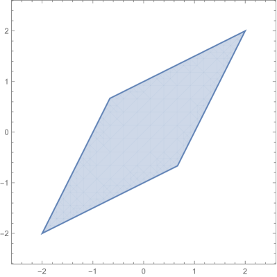
Figure 6: The set $\mathcal{M}$ for $C=\left(\begin{smallmatrix}1&-0.5\\ -0.5&1\end{smallmatrix}\right)$ and $\lambda_{0}=(1,1)^{\prime}$.

7 Summary and conclusion

We consider confidence regions based on the Lasso estimator covering the entire unknown parameter vector, thereby quantifying estimation uncertainty of this estimator. We provide exact formulas for the minimal coverage probability of these regions in finite samples and asymptotically in a low-dimensional framework when the estimator is tuned to perform conservative model selection. We do this without explicit knowledge of the distribution but by carefully exploiting the structure of the optimization problem that defines the estimator. The sets we consider as confidence regions need to satisfy certain shape constraints which apply to the regular confidence ellipse based on the LS estimator. We show that the LS confidence ellipse is always smaller than the one based on the Lasso estimator, but not contained in the Lasso ellipse in general. An ellipse is not the optimal shape for the confidence region based on the Lasso estimator in terms of volume. We give some guidelines on how to construct regions of smaller volume. We show how a set can be minimally enlarged in order to comply with the imposed shape condition, allowing to start the construction with sets of arbitrary shapes. We also illustrate how the coverage probability of the Lasso ellipse varies over the parameter space for the case when $p=2$, in which we also show how our results can be used for constructing valid confidence intervals for single components of the parameter space. In case the error variance needs to be estimated, our results involve non-central $t$-distributions rather than shifted normal distributions. Finally, in the consistently tuned case, we give a simple asymptotic confidence regions in the shape of a parallelogram that is determined by the regressor matrix.

Appendix A Proofs

We start the proof section with introducing some notation that will be used throughout this section. Let $e_{j}$ denote the $j^{\text{\tiny th}}$ unit vector in $\mathbb{R}^{p}$ and let $\iota=(1,\dots,1)^{\prime}\in\mathbb{R}^{p}$. For a vector $d\in\{-1,1\}^{p}$, we define $\mathcal{O}^{d}$ to be the corresponding orthant of $\mathbb{R}^{p}$, that is, $\mathcal{O}^{d}=\{z\in\mathbb{R}^{p}:d_{j}z_{j}\geq 0\}$ and $\bar{\mathcal{O}}^{d}$ to be the corresponding orthant of $\overline{\mathbb{R}}^{p}$, that is, $\bar{\mathcal{O}}^{d}=\{z\in\overline{\mathbb{R}}^{p}:d_{j}z_{j}\geq 0\}$. By $\mathcal{O}^{\iota}_{\text{\tiny int}}$ we denote the orthant with strictly positive components only, that is, $\mathcal{O}^{\iota}_{\text{\tiny int}}=\{z\in\mathbb{R}^{p}:z_{j}>0\}$. The sup-norm on $\mathbb{R}^{p}$ is denoted by $\|.\|_{\infty}$.

To remind the reader of some notation relevant for the following proofs that was introduced previously throughout the paper, note that $\hat{u}_{n}=n^{1/2}(\hat{\beta}_{\text{\tiny L}}-\beta)$, where $\hat{u}_{n}$ is the minimizer of $Q_{n}$, and $\hat{u}_{\text{\tiny LS}}=n^{1/2}(\hat{\beta}_{\text{\tiny LS}}-\beta)$. The minimizer of $Q_{n}^{d}$ was labeled $\hat{u}_{n}^{d}$. The asymptotic versions in the conservatively tuned case were labeled $\hat{u}$ and $Q$, as well as $\hat{u}^{d}$ and $Q^{d}$, respectively.

The directional derivative of a function $g:\mathbb{R}^{p}\to\mathbb{R}$ at $u$ in the direction of $r\in\mathbb{R}^{p}\setminus{\{0\}}$ is defined as

$$\frac{\partial g(u)}{\partial r}=\lim_{h\searrow 0}\frac{g(u+hr)-g(u)}{h}.$$

A.1 Proofs for Section 3

In order to prove the main theorem, we start by re-writing Condition A. For $m\in\mathbb{R}^{p}$ and a $p\times p$ matrix $\bar{C}$, we define

$$A^{d_{j}}_{\bar{C},j}(m) \;=\;\{z\in\mathbb{R}^{p}:d_{j}(\bar{C}m)_{j}\leq d_{j}(\bar{C}z)_{j},d_{j}z_{j}\leq 0\}\text{ and }$$

$$B^{d_{j}}_{\bar{C},j}(m) \;=\;\{z\in\mathbb{R}^{p}:(\bar{C}z)_{j}=(\bar{C}m)_{j},d_{j}z_{j}>0\}$$

for $j=1,\dots,p$. Note that clearly we have

$$A^{d}_{\bar{C}}(m)=\bigcap_{j=1}^{p}A^{d_{j}}_{\bar{C},j}(m),$$

and that, in fact, also the following lemma holds.

Lemma 15.

$$\bigcup_{d\in\{-1,1\}^{p}}\;\bigcap_{j=1}^{p}A^{d_{j}}_{\bar{C},j}(m)=\bigcup_{d\in\{-1,1\}^{p}}\;\bigcap_{j=1}^{p}A^{d_{j}}_{\bar{C},j}(m)\cup B^{d_{j}}_{\bar{C},j}(m)$$

Proof.

We fix $m$ and $\bar{C}$, drop the corresponding subscripts and show that the set on the left-hand side of the equation contains the set on the right-hand side of the equation. To this end, take any $z$ from the set on right-hand side. Then there exists a $d\in\{-1,1\}^{d}$ such that for each $j=1,\dots,p$, $z$ is either contained in $A^{d_{j}}_{j}$ or in $B^{d_{j}}_{j}$. We pick $f\in\{-1,1\}^{p}$ in the following way: if $z\in A^{d_{j}}_{j}$, set $f_{j}=d_{j}$ and if $z\in B^{d_{j}}_{j}$, set $f_{j}=-d_{j}$. Then, by construction, $z\in A^{f}_{j}$ for all $j=1,\dots,p$ and therefore $z\in\bigcap_{j}A^{f}_{j}$ so that $z$ is contained in the set on the left-hand side of the equation. ∎

Since needed later on, we also prove the following proposition which quantifies the maximal distance between the Lasso and the LS estimator in finite samples.

Proposition 16.

For each $j=1,\dots,p$, we have

$$\left|(X^{\prime}X(\hat{\beta}_{\text{\tiny L}}-\hat{\beta}_{\text{\tiny LS}}))_{j}\right|\leq\lambda_{n,j},$$

or, equivalently,

$$\left|\left(C_{n}(\hat{u}_{n}-\hat{u}_{\text{\tiny LS}})\right)_{j}\right|\leq n^{-1/2}\lambda_{n,j},$$

where $\hat{u}_{\text{\tiny LS}}=n^{1/2}(\hat{\beta}_{\text{\tiny LS}}-\beta)$.

Proof.

The two inequalities above just differ by a scaling factor. We show the latter one. We have $W_{n}=n^{-1/2}X^{\prime}\varepsilon=C_{n}\hat{u}_{\text{\tiny LS}}$. Consider the directional derivative of $Q_{n}$ at its minimizer $\hat{u}_{n}$ in the direction of $e_{j}$ and $-e_{j}$. We have

$$0\;\leq\;\frac{\partial}{\partial e_{j}}Q_{n}(\hat{u}_{n}) \;=\;2(C_{n}\hat{u}_{n})_{j}-2W_{n,j}+2n^{-1/2}\lambda_{n,j}\left[\mathds{1}_{\{\hat{u}_{j}\geq-n^{1/2}\beta_{j}\}}-\mathds{1}_{\{\hat{u}_{j}<-n^{1/2}\beta_{j}\}}\right]$$

$$\;\leq\;2(C_{n}\hat{u}_{n})_{j}-2(C_{n}\hat{u}_{\text{\tiny LS}})_{j}+2n^{-1/2}\lambda_{n,j},$$

as well as

$$0\;\leq\;\frac{\partial}{\partial(-e_{j})}Q_{n}(\hat{u}_{n}) \;=\;-2(C_{n}\hat{u}_{n})_{j}+2W_{n,j}+2n^{-1/2}\lambda_{n,j}\left[\mathds{1}_{\{\hat{u}_{j}\leq-n^{1/2}\beta_{j}\}}-\mathds{1}_{\{\hat{u}_{j}>-n^{1/2}\beta_{j}\}}\right]$$

$$\;\leq\;-2(C_{n}\hat{u}_{n})_{j}+2(C_{n}\hat{u}_{\text{\tiny LS}})_{j}+2n^{-1/2}\lambda_{n,j}.$$

Piecing the two displays above together yields the second inequality in the proposition. ∎

To proceed note that $Q_{n}^{d}$ as defined in (1) is a simple quadratic and strictly convex function in $u$ with unique minimizer $\hat{u}_{n}^{d}$ given by

$$\hat{u}_{n}^{d}=C_{n}^{-1}(W_{n}-n^{-1/2}\Lambda_{n}d),$$ (5)

where $W_{n}\sim N(0,\sigma^{2}C_{n})$. We first show Theorem 1 for one orthant of the parameter space $\mathbb{R}^{p}$, as is formulated in Proposition 17.

Proposition 17.

If $M_{n}\subseteq\mathbb{R}^{p}$ satisfies that

$$\bigcap_{j=1}^{p}A^{\iota_{j}}_{C_{n},j}(m)\cup B^{\iota_{j}}_{C_{n},j}(m)\subseteq M_{n}$$

for all $m\in M_{n}$, then

$$\inf_{\beta\in\mathcal{O}^{\iota}}P_{\beta}(\hat{u}_{n}\in M_{n})=P(\hat{u}_{n}^{\iota}\in M_{n}).$$

In essence, Proposition 17 states Theorem 1 for the orthant of the parameter space where all components of $\beta$ are non-negative. The condition in Proposition 17 takes the role of Condition A for the corresponding orthant, as will become apparent later on in the proof of Theorem 1.

Proof of Proposition 17.

We first show that $\inf_{\beta\in\mathcal{O}^{\iota}}P_{\beta}(\hat{u}_{n}\in M_{n})\geq P(\hat{u}_{n}^{\iota}\in M_{n})$ by showing that for each fixed $\omega\in\Omega$, $\hat{u}_{n}^{\iota}\in M_{n}$ implies that $\hat{u}_{n}\in M_{n}$ as long as $\beta_{j}\geq 0$ for all $j$. For this, we first show the following two facts.

1. $(C_{n}\hat{u}_{n}^{\iota})_{j}\leq(C_{n}\hat{u}_{n})_{j}$ for all $j=1,\dots,p$.

   Suppose there exists a $j_{0}$ with such that $(C_{n}\hat{u}_{n}^{\iota})_{j_{0}}>(C_{n}\hat{u}_{n})_{j_{0}}$ and note that by (5) we have $(C_{n}\hat{u}_{n}^{\iota})_{j}=W_{n,j}-n^{-1/2}\lambda_{n,j}$ for each $j=1,\dots,p$. Now consider the directional derivative of $Q_{n}$ at its minimizer $\hat{u}_{n}$ in direction $e_{j_{0}}$,

   $$\frac{\partial Q_{n}(\hat{u}_{n})}{\partial e_{j_{0}}} \;=\;2(C_{n}\hat{u}_{n})_{j_{0}}-2W_{n,j_{0}}+2n^{-1/2}\lambda_{n,j_{0}}\left[\mathds{1}_{\{\hat{u}_{n,j_{0}}\geq-n^{1/2}\beta_{j_{0}}\}}-\mathds{1}_{\{\hat{u}_{n,j_{0}}<-n^{1/2}\beta_{j_{0}}\}}\right]$$

   $$\;\leq\;2(C_{n}\hat{u}_{n})_{j_{0}}-2W_{n,j_{0}}+2n^{-1/2}\lambda_{n,j_{0}}$$

   $$\;=\;2(C_{n}\hat{u}_{n})_{j_{0}}-2(C_{n}\hat{u}_{n}^{\iota})_{j_{0}}<0,$$

   which is a contradiction to $\hat{u}_{n}$ minimizing $Q_{n}$.

2. $\hat{u}_{n,j}>0$ implies $(C_{n}\hat{u}_{n})_{j}=(C_{n}\hat{u}_{n}^{\iota})_{j}$ for any $1\leq j\leq p$.

   If $\hat{u}_{n,j}>0$ (and hence $\hat{u}_{n,j}+n^{1/2}\beta_{j}>0$ when $\beta_{j}\geq 0$), then $Q_{n}$ is partially differentiable at $\hat{u}_{n}$ with respect to the $j^{\text{\tiny th}}$ component. Therefore, we have

   $$\frac{\partial Q_{n}(\hat{u}_{n})}{\partial u_{j}} \;=\;2(C_{n}\hat{u}_{n})_{j}-2W_{n,j}+2n^{1/2}\lambda_{n,j}$$

   $$\;=\;2(C_{n}\hat{u}_{n})_{j}-2(C_{n}\hat{u}_{n}^{\iota})_{j}=0.$$

Now, by Facts (a) and (b) we clearly have that $\hat{u}_{n}\in A_{C_{n}}^{\iota_{j}}(\hat{u}_{n}^{\iota})\cup B_{C_{n}}^{\iota_{j}}(\hat{u}_{n}^{\iota})$. So, by assumption, $\hat{u}_{n}^{\iota}\in M_{n}$ clearly implies $\hat{u}_{n}\in M_{n}$ as long as $\beta_{j}\geq 0$ for all $j$. We have therefore shown that

$$\inf_{\beta\in\mathcal{O}^{\iota}}P_{\beta}(\hat{u}_{n}\in M_{n})\geq P(\hat{u}^{\iota}_{n}\in M_{n}).$$

To see the reverse inequality, note that if $\hat{u}_{n,j}+n^{1/2}\beta_{j}>0$ for all $j$, then $Q_{n}$ is differentiable at $\hat{u}_{n}$ and

$$\frac{\partial Q_{n}(\hat{u}_{n})}{\partial u}=2C_{n}\hat{u}_{n}-2W_{n}+2n^{-1/2}\lambda_{n}=2C_{n}\hat{u}_{n}-2C_{n}\hat{u}_{n}^{\iota}=0,$$

implying that $\hat{u}_{n}=\hat{u}_{n}^{\iota}$. Also note that $\hat{u}_{n,j}+n^{1/2}\beta_{j}>0$ for each $j$ is equivalent to $\hat{\beta}_{\text{\tiny L}}\in\mathcal{O}^{\iota}_{\text{\tiny int}}$, so that

$$\{\hat{u}_{n}\in M_{n}\}\subseteq\{\hat{u}_{n}^{\iota}\in M_{n}\}\cup\{\hat{\beta}_{\text{\tiny L}}\notin\mathcal{O}^{\iota}_{\text{\tiny int}}\}.$$

Now let $\kappa$ be a bound in the sup-norm on the set $\{z\in\mathbb{R}^{p}:\|C_{n}z\|_{\infty}\leq n^{-1/2}\|\lambda_{n}\|_{\infty}\}$ and for an arbitrary $\varepsilon>0$, pick $\beta^{*}\in\mathbb{R}^{p}$ such that $P(\hat{u}_{\text{\tiny LS}}\leq\kappa\iota-n^{1/2}\beta^{*})\leq\varepsilon$, where $\hat{u}_{\text{\tiny LS}}=n^{1/2}(\hat{\beta}_{\text{\tiny LS}}-\beta^{*})\sim N(0,\sigma^{2}C_{n}^{-1})$. Note that by Proposition 16, this implies that

$$P_{\beta^{*}}(\hat{\beta}_{\text{\tiny L}}\leq 0)=P_{\beta^{*}}(\hat{u}_{n}-\hat{u}_{\text{\tiny LS}}+\hat{u}_{\text{\tiny LS}}\leq-n^{1/2}\beta^{*})\leq P_{\beta^{*}}(-\kappa\iota+\hat{u}_{\text{\tiny LS}}\leq-n^{1/2}\beta^{*})\leq\varepsilon,$$

yielding

$$\inf_{\beta\in O^{\iota}}P_{\beta}(\hat{u}_{n}\in M_{n})\leq P_{\beta^{*}}(\hat{u}_{n}\in M_{n})\leq P(\hat{u}^{\iota}_{n}\in M_{n})+\varepsilon.$$

Since $\varepsilon>0$ was arbitrary, this shows the desired inequality. ∎

Essentially, we have now shown the main theorem for one part of the parameter space $\mathbb{R}^{p}$. By flipping signs, we can apply Proposition 17 to each orthant $\mathcal{O}^{d}$, thus obtaining the formula for the infimal coverage over the whole space.

Proof of Theorem 1.

First note that

$$\inf_{\beta\in\mathbb{R}^{p}}P_{\beta}(\hat{u}_{n}\in M_{n})=\min_{d\in\{-1,1\}^{p}}\inf_{\beta\in\mathcal{O}^{d}}P_{\beta}(\hat{u}_{n}\in M_{n}).$$

Thus, if we can show that

$$\inf_{\beta\in\mathcal{O}^{d}}P_{\beta}(\hat{u}_{n}\in M_{n})=P(\hat{u}_{n}^{d}\in M_{n})$$

for each $d\in\{-1,1\}^{p}$, the proof is done. Now, fix $d$ and set $D=\operatorname{diag}(d)$. We consider the function

$$\tilde{Q}_{n}(u)=Q_{n}(Du) \;=\;u^{\prime}DC_{n}Du-2u^{\prime}DW_{n}+2n^{-1/2}\sum_{j=1}^{p}\lambda_{n,j}\left[|d_{j}u_{j}+n^{1/2}\beta_{j}|-|n^{1/2}\beta_{j}|\right]$$

$$\;=\;u^{\prime}\tilde{C}_{n}u-2u^{\prime}\tilde{W}_{n}+2n^{-1/2}\sum_{j=1}^{p}\lambda_{n,j}\left[|u_{j}+n^{1/2}d_{j}\beta_{j}|-|n^{1/2}d_{j}\beta_{j}|\right],$$

where $\tilde{C}_{n}=DC_{n}D$, $\tilde{W}_{n}=DW_{n}\sim N(0,\sigma^{2}\tilde{C}_{n})$. We write $\tilde{u}_{n}$ for the minimizer of $\tilde{Q}_{n}$, and, analogously to Section 3, we define $\tilde{u}_{n}^{\iota}$ to be the minimizer of the function $u^{\prime}\tilde{C}_{n}u-2u^{\prime}\tilde{W}_{n}+2n^{-1/2}\sum_{j=1}^{p}\lambda_{n,j}u_{j}$.

If we can show that the set $DM_{n}$ satisfies the requirement of Proposition 17 with the matrix $\tilde{C}_{n}$ in place of $C_{n}$, we may conclude that

$$\inf_{\beta:d_{j}\beta_{j}\geq 0}P_{\beta}(\tilde{u}_{n}\in DM_{n})=P(\tilde{u}_{n}^{\iota}\in DM_{n}).$$

Note that $\hat{u}_{n}=D\tilde{u}_{n}$, $\hat{u}_{n}^{d}=D\tilde{u}_{n}^{\iota}$ and $D^{-1}=D$, so that

$$\inf_{\beta\in\mathcal{O}^{d}}P(\hat{u}_{n}\in M_{n})=\inf_{\beta\in\mathcal{O}^{d}}P(\tilde{u}_{n}\in DM_{n})=P(\tilde{u}_{n}^{\iota}\in DM_{n})=P(\hat{u}_{n}^{d}\in M_{n}),$$

which proves the formula for the infimal coverage probability. We now show that the set $DM_{n}$ satisfies that

$$\bigcap_{j=1}^{p}A^{\iota}_{\tilde{C}_{n},j}(Dm)\cup B^{\iota}_{\tilde{C}_{n},j}(Dm)\subseteq DM_{n}$$

for all $m\in M_{n}$. A straightforward calculation shows that this is equivalent to

$$\bigcap_{j=1}^{p}A^{d_{j}}_{C_{n},j}(m)\cup B^{d_{j}}_{C_{n},j}(m)\subseteq M_{n}$$

for each $m\in M$ which clearly holds by Condition A and Proposition 15.

The distributional result on $\hat{u}_{n}^{d}$ immediately follows by (5). ∎

A.2 Proofs for Section 4

Proof of Proposition 3.

Let $m\in E_{C_{n}}(k)$ and $y\in A_{C_{n}}^{d}(m)$. We show that $y\in E_{C_{n}}(k)$. Remember that $D=\operatorname{diag}(d)$ satisfies $DD=I_{p}$. Since $y\in A_{C_{n}}^{d}(m)$ we have $-Dy\in\mathcal{O}^{\iota}$ and $-DC(m-y)\in\mathcal{O}^{\iota}$ implying that

$$y^{\prime}C(m-y)=(Dy)^{\prime}DC(m-y)\geq 0.$$

Furthermore, since $(m-y)^{\prime}C(m-y)\geq 0$, we have

$$m^{\prime}C(m-y)\geq y^{\prime}C(m-y)\geq 0,$$

which in turn yields

$$m^{\prime}Cm\geq m^{\prime}Cy\geq y^{\prime}Cy\geq 0.$$

But this means that $k\geq m^{\prime}Cm\geq m^{\prime}Cy\geq y^{\prime}Cy$ and therefore $y\in E_{C_{n}}(k)$. ∎

Proof of Proposition 4.

We transform the ellipse to a sphere and the corresponding normal distribution to have independent components with equal variances.

$$P\left(\hat{u}^{d}_{n}\in E_{C_{n}}(k)\right)=P\left(C_{n}^{1/2}\hat{u}^{d}_{n}\in C_{n}^{1/2}E_{C_{n}}(k)\right),$$

where $C_{n}^{1/2}\hat{u}^{d}_{n}\sim N(-n^{-1/2}C_{n}^{-1/2}\Lambda_{n}d,\sigma^{2}I_{p})$ and $C_{n}^{1/2}E_{C_{n}}(k)=\{z\in\mathbb{R}^{p}:\|z\|^{2}\leq k\}$. So clearly, the smallest probability will be achieved for the distribution with mean furthest away from the origin, which is any $d^{*}$ maximizing $\|C_{n}^{-1/2}\Lambda_{n}d\|$ over all $d\in\{-1,1\}^{p}$. ∎

Proof of Proposition 5.

Similarly to the proof of Proposition 4, note that

$$P\left(\hat{u}^{d}_{n}\in E_{C_{n}}(k)\right)=P\left(C_{n}^{1/2}\hat{u}^{d}_{n}/\sigma\in C_{n}^{1/2}E_{C_{n}}(k)/\sigma\right)$$

with $\hat{w}=C_{n}^{1/2}\hat{u}^{d}_{n}/\sigma\sim N(-n^{-1/2}C_{n}^{-1/2}\Lambda_{n}d/\sigma,I_{p})$ and $C_{n}^{1/2}E_{C_{n}}(k)/\sigma=\{z\in\mathbb{R}^{p}:\|z\|^{2}\leq k/\sigma^{2}\}$. Therefore, the probability in the above display is given by

$$P(\|\hat{w}\|^{2}\leq k/\sigma^{2})$$

where $\|\hat{w}\|^{2}$ clearly follows the claimed non-central $\chi^{2}$-distribution. ∎

Proof of Proposition 6.

We start by showing that for any $m\in\mathbb{R}^{p}$, $d\in\{-1,1\}^{p}$, we have

$$A^{d}_{\bar{C}}(y)\subseteq A^{d}_{\bar{C}}(m)\;\;\;\text{for all }y\in A^{d}_{\bar{C}}(m).$$ (6)

Let $z\in A^{d}_{\bar{C}}(y)$. Then $d_{j}z_{j}\leq 0$ and $(\bar{C}y)_{j}\leq(\bar{C}z)_{j}$ for all $j$. But since $y\in A^{d}_{\bar{C}}(m)$, we also have $(\bar{C}m)_{j}\leq(\bar{C}y)_{j}$ for all $j$ so that that $(\bar{C}m)_{j}\leq(\bar{C}z)_{j}$ for all $j$ and therefore $z\in A^{d}_{\bar{C}}(m)$, thus proving (6). So clearly, the set

$$\bigcup_{m\in M}\bigcup_{d\in\{-1,1\}^{p}}A^{d}_{\bar{C}}(m)$$

satisfies Condition A. For each $m\in M$, choose $d\in\{-1,1\}^{p}$ in such a way that $d_{j}=1$ if $m_{j}=0$ and $d_{j}=-\operatorname{sgn}(m_{j})$ for $m_{j}\neq 0$. We then get $m\in A^{d}_{\bar{C}}(m)$, implying that the set in the display above actually contains $M$. ∎

A.3 Proofs for Section 5

Proof of Proposition 8.

We start by proving that $M$ satisfies Condition A. For this, we need to show that for $d\in\{-1,1\}^{2}$, we have $A_{C_{n}}^{d}(m)=A_{C_{n}}^{d}(m)\cap\mathcal{O}^{-d}\subseteq M^{-d}$ for all $m\in M$. We start by doing so $d=(1,1)^{\prime}$. Note that

$$A^{(1,1)}_{C_{n}}(m)=\{z\in\mathcal{O}^{-(1,1)}:(Cm)_{j}\leq(Cz)_{j},j=1,2\}$$

and

$$M^{-(1,1)}=\{m\in\mathcal{O}^{-(1,1)}:-(C\underline{a})_{1}\leq(Cm)_{1}\}\subseteq\tilde{M}.$$

If $m\in M^{-(1,1)}$, then clearly $-(C\underline{a})_{1}\leq(Cm)_{1}\leq(Cz)_{1}$ for any $z\in A^{(1,1)}_{C_{n}}(m)$, so that $z\in M^{-(1,1)}$ follows. If $m\in M^{(1,1)}$, then $A^{(1,1)}_{C_{n}}(m)=\varnothing$ unless $m=0$, in which case $A^{(1,1)}_{C_{n}}(0)=\{0\}$. In either case, $A^{(1,1)}_{C_{n}}(m)\subseteq M^{-(1,1)}$ follows immediately. If $m\in M^{(-1,1)}\subseteq\{m\in\mathbb{R}^{2}:-a\leq m_{1}\leq 0$, $m_{2}\leq 0\}$, we have $-(C\underline{a})_{1}=-c_{11}a\leq c_{11}m_{1}+c_{12}m_{2}=(Cm)_{1}\leq(Cz)_{1}$ for any $z\in A^{(1,1)}_{C_{n}}(m)$, so that $z\in M^{-(1,1)}$ again follows. Finally, if $m\in M^{(1,-1)}\subseteq\{m\in\mathcal{O}^{(1,-1)}:-c_{11}c_{22}a/c_{12}\leq(Cm)_{2}\}$, we have $-c_{11}a\leq c^{2}_{12}/(c_{11}c_{22})\,c_{11}m_{1}+c_{12}m_{2}\leq(Cm)_{1}\leq(Cz)_{1}$ for any $z\in A^{(1,1)}_{C_{n}}(m)$, so that $z\in M^{-(1,1)}$ follows yet again.

The remaining cases $d=-(1,1)^{\prime}$, $d=(-1,1)^{\prime}$ and $d=(1,-1)^{\prime}$ can be shown in a similar manner.

To show the second part of Proposition 8, assume there exists $\bar{m}\in\bar{M}$ with $\bar{m}\notin M$ and show that this implies $\max_{m\in\bar{M}}|m_{1}|>a$ if $\bar{M}$ complies with Condition A. If $\bar{m}\in\mathcal{O}^{(1,1)}$, then $\bar{m}\notin M^{(1,1)}$ entails that $c_{11}\bar{m}_{1}+c_{12}\bar{m}_{2}=(C\bar{m})_{1}>(C\underline{a})_{1}=c_{11}a$. Let $\bar{\underline{a}}=(\bar{a},0)^{\prime}$ where $\bar{a}=\bar{m}_{1}+c_{12}\bar{m}_{2}/c_{11}>a$ and note that $\bar{\underline{a}}\in A^{-(1,1)}_{C_{n}}\subseteq\bar{M}$ which implies that $\max_{m\in\bar{M}}|m_{1}|\geq\bar{a}>a$ The remaining cases $\bar{m}\in\mathcal{O}^{-(1,1)}$, $\bar{m}\in\mathcal{O}^{(-1,1)}$ and $\bar{m}\in\mathcal{O}^{(1,-1)}$ can be shown in a similar manner. ∎

A.4 Proofs for Section 6

Proof of Remark 2.

We show (2). Note that Proposition 16 entails that

$$\hat{\beta}_{\text{\tiny L}}\in\hat{\beta}_{\text{\tiny LS}}-\frac{1}{n^{1/2}}B_{n},$$

where

$$B_{n}=\{z\in\mathbb{R}^{p}:|(C_{n}z)_{j}|\leq n^{-1/2}\lambda_{n,j}\text{ for }j=1,\dots,p\}.$$

Since $\lambda_{n}/n^{1/2}$ converges, we have $B_{n}\subseteq C_{n}^{-1}\bar{B}_{\delta}$ with $\bar{B}_{\delta}=\{x\in\mathbb{R}^{p}:\|x\|_{\infty}\leq\delta\}$ for some $\delta>0$. Since $C_{n}^{-1}\to C^{-1}$, the set $\{C_{n}^{-1}:n\in\mathbb{N}\}$ is bounded in operator sup-norm by Banach-Steinhaus, so that the set $B_{n}$ is uniformly bounded over $n$ in sup-norm by, say, $\gamma>0$. We now fix a component $j$ and show that $\liminf_{n\to\infty}\inf_{\beta\in\mathbb{R}^{p}}P_{\beta}(\hat{\beta}_{{\text{\tiny L}},j}\neq 0)>0$. To this end, define $\mathcal{R}_{j}=\mathbb{R}^{j-1}\times\{0\}\times\mathbb{R}^{p-j}$. Let $\xi^{2}_{j,n}$ and $\xi^{2}_{j}$ be the positive $j^{\text{\tiny th}}$ diagonal element of $C_{n}^{-1}$ and $C^{-1}$, respectively. Observe that

$$\inf_{\beta\in\mathbb{R}^{p}}P_{\beta}(\hat{\beta}_{{\text{\tiny L}},j}\neq 0) \;\geq\;\inf_{\beta\in\mathbb{R}^{p}}P_{\beta}\left((\hat{\beta}_{\text{\tiny LS}}-\frac{1}{n^{1/2}}B_{n})\cap\mathcal{R}_{j}=\varnothing\right)$$

$$\;\geq\;\inf_{\beta\in\mathbb{R}^{p}}P_{\beta}(n^{1/2}\hat{\beta}_{{\text{\tiny LS}},j}+\gamma<0\text{ or }n^{1/2}\hat{\beta}_{{\text{\tiny LS}},j}-\gamma>0)$$

$$\;=2\Phi(-\gamma/\xi_{i,n})\longrightarrow 2\Phi(-\gamma/\xi_{i})>0$$

∎

In order to prove Theorem 10, we need an asymptotic version of Proposition 17 which is formulated in the following.

Proposition 18.

If $M\subseteq\mathbb{R}^{p}$ satisfies that

$$\bigcap_{j=1}^{p}A^{\iota_{j}}_{C,j}(m)\cup B^{\iota_{j}}_{C,j}(m)\subseteq M$$

for all $m\in M_{n}$, then

$$\inf_{t\in\bar{\mathcal{O}}^{\iota}}P_{t}(\hat{u}\in M)=P(\hat{u}^{\iota}\in M).$$

Proof.

The first part of the proof is completely analogous to the first part of the proof of Proposition 17 after identifying $n^{1/2}\beta$ with $t$ and dropping the subscript $n$. To see the reverse inequality, note that for $t^{*}=(\infty,\dots,\infty)\in\overline{\mathbb{R}}^{p}$, we actually have $Q=Q^{\iota}$, so that $\hat{u}=\hat{u}^{\iota}$ in this case which already yields that

$$\inf_{t\in\bar{O}^{\iota}}P_{t}(\hat{u}\in M)\leq P_{t^{*}}(\hat{u}\in M)=P(\hat{u}^{\iota}\in M).$$

∎

Proof of Theorem 10.

The proof again is completely analogous to the proof of Theorem 1 after identifying $n^{1/2}\beta$ with $t$, dropping the subscript $n$ everywhere and using Proposition 18 instead of Proposition 17. Also, replace $\mathcal{O}^{d}$ by $\bar{\mathcal{O}}^{d}$ and note that

$$Q^{d}(u) \;=\;Q(Du)=u^{\prime}DCDu-2u^{\prime}DW+2\sum_{i=1}^{p}\lambda_{j}\left[\mathds{1}_{\{t_{j}\in\mathbb{R}\}}(|t_{j}+d_{j}u_{j}|-|t_{j}|)+\mathds{1}_{\{|t_{j}|=\infty\}}\operatorname{sgn}(t_{j})d_{j}u_{j}\right]$$

$$\;=\;u^{\prime}\tilde{C}u-2u^{\prime}\tilde{W}+2\sum_{i=1}^{p}\lambda_{j}\left[\mathds{1}_{\{d_{j}t_{j}\in\mathbb{R}\}}(|u_{j}+d_{j}t_{j}|-|d_{j}t_{j}|)+\mathds{1}_{\{|d_{j}t_{j}|=\infty\}}\operatorname{sgn}(d_{j}t_{j})u_{j}\right],$$

where $\tilde{C}=DCD$ and $\tilde{W}=DW$. ∎

Proof of Corollary 11.

Let $c=\liminf_{n\to\infty}\inf_{\beta\in\mathbb{R}^{p}}P_{\beta}(\beta\in\hat{\beta}_{\text{\tiny L}}-n^{-1/2}M)$. Then there exists a sequence $\beta_{n}$ in $\mathbb{R}^{p}$ such that $P_{\beta_{n}}(\beta_{n}\in\hat{\beta}_{\text{\tiny L}}-n^{-1/2}M)\to c$. Assume that $n^{1/2}\beta_{n}\to t\in\overline{\mathbb{R}}^{p}$ (if the sequence does not converge, pass to subsequences). Since

$$P_{\beta_{n}}(\beta_{n}\in\hat{\beta}_{\text{\tiny L}}-n^{-1/2}M)=P_{\beta_{n}}(n^{1/2}(\hat{\beta}_{\text{\tiny L}}-\beta_{n})\in M)\longrightarrow c=P_{t}(\hat{u}\in M)$$

as $n\to\infty$ in the notation of Proposition 9. Theorem 10 then yields $c\geq\min_{d\in\{-1,1\}^{p}}P(\hat{u}^{d}\in M)=1-\alpha$. To see the reverse inequality, let $\beta_{n}=d\in\{-1,1\}^{p}$ and note that for this sequence, we have

$$P_{\beta_{n}}(\beta_{n}\in\hat{\beta}_{\text{\tiny L}}-n^{-1/2}M)=P_{\beta_{n}}(n^{1/2}(\hat{\beta}_{\text{\tiny L}}-\beta_{n})\in M)\longrightarrow P_{t}(\hat{u}\in M)$$

as $n\to\infty$, where $t=(d_{1}\infty,\dots,d_{p}\infty)^{\prime}\in\overline{\mathbb{R}}^{p}$. Note that for this choice of $t$, $P_{t}(\hat{u}\in M)=P(\hat{u}^{d}\in M)$. Since $d\in\{-1,1\}^{p}$ was arbitrary, $c\leq\min_{d\in\{-1,1\}^{p}}P(\hat{u}^{d}\in M)=1-\alpha$ follows. ∎

Proof of Proposition 12.

Define the function $V_{n}(u)=n[L_{n}(\beta_{n}+\lambda_{n}^{*}u/n)-L_{n}(\beta_{n})]/(\lambda_{n}^{*})^{2}$ and note that $V_{n}$ is minimized at $n(\hat{\beta}_{\text{\tiny L}}-\beta_{n})/\lambda^{*}_{n}$. The function $V_{n}$ is then given by

$$V_{n}(u)=u^{\prime}\frac{X^{\prime}X}{n}u-2\frac{1}{\lambda^{*}_{n}}u^{\prime}X^{\prime}\varepsilon+2\sum_{j=1}^{p}\frac{\lambda_{n,j}}{\lambda_{n}^{*}}\left[\Big{|}u_{j}+\frac{n}{\lambda^{*}_{n}}\beta_{n,j}\Big{|}-\Big{|}\frac{n}{\lambda^{*}_{n}}\beta_{n,j}\Big{|}\right].$$

Clearly $u^{\prime}X^{\prime}Xu/n\to u^{\prime}Cu$ by assumption. Since $X^{\prime}\varepsilon/\lambda_{n}^{*}=(n^{1/2}/\lambda_{n}^{*})X^{\prime}\varepsilon/n^{1/2}$ and $\lambda_{n}^{*}/n^{1/2}\to\infty$ as well as $X^{\prime}\varepsilon/n^{1/2}=O_{P}(1)$, the second term in the above display vanishes in probability. To treat the third term, simply note that $\lambda_{n,j}/\lambda_{n}^{*}\to\lambda_{0,j}\in[0,1]$ and $n\beta_{n,j}/\lambda_{n}^{*}\to\zeta_{i}\in\overline{\mathbb{R}}$ by assumption. Piecing this together yields

$$V_{n}(u)\overset{p}{\longrightarrow}u^{\prime}Cu+2\sum_{j=1}^{p}\lambda_{0,j}\left[\mathds{1}_{\{\zeta_{j}\in\mathbb{R}\}}(|u_{j}+\zeta_{j}|-|\zeta_{j}|)+\mathds{1}_{\{|\zeta_{j}|=\infty\}}\operatorname{sgn}(\zeta_{j})u_{j}\right]=V^{\zeta}(u).$$

Since $V_{n}$ and $V^{\zeta}$ are strictly convex and $V^{\zeta}$ is non-random, it follows by Geyer (1996) that also the corresponding minimizers converge in probability to the minimizer of the limiting function. ∎

Proof of Proposition 13.

The equality of the two sets given in the display of Proposition 13 is trivial. We show that the set $\mathcal{M}$ as defined in (4) is equal to the set on the left-hand side and start by proving that $\mathcal{M}$ is contained in that set. Take any $m\in\mathcal{M}$, by definition, there exists a $\zeta\in\overline{\mathbb{R}}^{p}$ so that $m$ is the minimizer of $V^{\zeta}$. We need to show that $|(Cm)_{j}|\leq\lambda_{0,j}$ for all $j$. Assume that $|(Cm)_{j_{0}}|>\lambda_{0,j_{0}}$ for some $1\leq j_{0}\leq p$. If $(Cm)_{j_{0}}>\lambda_{0,j_{0}}$ we consider the directional derivative of $V^{\zeta}$ at its minimizer $m$ in the direction of $-e_{j_{0}}$ to get

$$\frac{\partial V^{\zeta}(m)}{\partial(-e_{j_{0}})} \;=\;-2(Cm)_{j}+2\lambda_{0,j_{0}}\left[\mathds{1}_{\{m_{j}+\zeta_{j}\leq 0\}}-\mathds{1}_{\{m_{j}+\zeta_{j}>0\}}\right]$$

$$\;\leq\;-2(Cm)_{j}+2\lambda_{0,j_{0}}<0,$$

which is a contradiction to $m$ minimizing $V^{\zeta}$. If $(Cm)_{j_{0}}<-\lambda_{0,j_{0}}$, then consider the directional derivative of $V^{\zeta}$ at $m$ in the direction of $e_{j_{0}}$ to arrive at

$$\frac{\partial V^{\zeta}(m)}{\partial e_{j_{0}}} \;=\;2(Cm)_{j}+2\lambda_{0,j_{0}}\left[\mathds{1}_{\{m_{j}+\zeta_{j}\geq 0\}}-\mathds{1}_{\{m_{j}+\zeta_{j}<0\}}\right]$$

$$\;\leq\;-2(Cm)_{j}+2\lambda_{0,j_{0}}<0,$$

yielding a contradiction also.

To see the reverse set-inclusion, we need to show that for any $m\in\mathbb{R}^{p}$ satisfying $|(Cm)_{j}|\leq\lambda_{0,j}$ for all $j=1,\dots,p$, there exists a $\zeta\in\overline{\mathbb{R}}^{p}$ such that $m$ is the minimizer of $V^{\zeta}$. Let $\zeta=-m\in\mathbb{R}^{p}$ and consider the directional derivative of $V^{\zeta}$ at $m$ in any direction $r\in\mathbb{R}^{p}\setminus\{0\}$:

$$\frac{\partial V^{\zeta}(m)}{\partial r}=2r^{\prime}Cm+2\sum_{j=1}^{p}\lambda_{0,j}|r_{j}|\geq\sum_{j=1}^{p}-2|(Cm)_{j}r_{j}|+2\lambda_{0,j}|r_{j}|=2\sum_{j=1}^{p}\left[-|(Cm)_{j}|+\lambda_{0,j}\right]|r_{j}|\geq 0.$$

Since the directional derivative is non-negative in any direction $r\in\mathbb{R}^{p}\setminus\{0\}$ and $V^{\zeta}$ is (strictly) convex, $m$ must be the minimizer. ∎

Proof of Corollary 14.

We start with the case $d>1$. Let $c=\liminf_{n\to\infty}\inf_{\beta\in\mathbb{R}^{p}}P_{\beta}(\beta\in\hat{\beta}_{\text{\tiny L}}-d\lambda_{n}^{*}\mathcal{M}/n)$. By definition, there exists a subsequence $n_{k}$ and elements $\beta_{n_{k}}\in\mathbb{R}^{p}$ such that

$$P_{\beta_{n_{k}}}\left(\beta_{n_{k}}\in\hat{\beta}_{\text{\tiny L}}-d\frac{\lambda_{n_{k}}^{*}}{n_{k}}\mathcal{M}\right)=P_{\beta_{n_{k}}}\left(\frac{n_{k}}{\lambda_{n_{k}}^{*}}(\hat{\beta}_{\text{\tiny L}}-\beta_{n_{k}})\in d\mathcal{M}\right)\longrightarrow c$$

as $k\to\infty$. Note that $d\mathcal{M}=\{m\in\mathbb{R}^{p}:|(Cm)_{j}|\leq d\lambda_{0,j},1\leq j\leq p\}$. Now, pick a further subsequence $n_{k_{l}}$ such that $\lambda^{*}_{n_{k_{l}}}\beta_{n_{k_{l}}}/n_{k_{l}}$ converges in $\overline{\mathbb{R}}^{p}$ to, say, $\zeta$. Proposition 12 then shows that $n_{k_{l}}(\hat{\beta}_{\text{\tiny L}}-\beta_{n_{k_{l}}})/\lambda^{*}_{n_{k_{l}}}$ converges in probability to the unique minimizer of $V^{\zeta}$ as $l\to\infty$. Finally, Proposition 13 implies that $c=1$.

We next look the case where $d<1$. Let $m=C^{-1}\lambda_{0}$ so that $m\in\mathcal{M}\setminus d\mathcal{M}$. From the proof of Proposition 13, we know that for $\zeta=-m$ we have $m=\operatorname*{\arg\min}_{u\in\mathbb{R}^{p}}V^{\zeta}(u)$. Let $\beta_{n}=n\zeta/\lambda^{*}_{n}$. By Proposition 12, $n(\hat{\beta}_{\text{\tiny L}}-\beta_{n})/\lambda^{*}_{n}$ converges to $m$ in $P_{\beta_{n}}$-probability, so that $P_{\beta_{n}}(n(\hat{\beta}_{\text{\tiny L}}-\beta_{n})/\lambda^{*}_{n}\in d\mathcal{M})\to 0$. ∎

References

- (1)
- Alliney & Ruzinsky (1994) Alliney S., Ruzinsky A. (1994). ‘An Algorithm for the Minimization of Mixed and Norms with Applications to Bayesian Estimation’. IEEE Transactions on Signal Processing 42:618–627.
- Berk et al. (2013) Berk R., et al. (2013). ‘Valid post-selection inference’. Annals of Statistics 41:802–837.
- Caner & Kock (2018) Caner M., Kock A. B. (2018). ‘Asymptotically Honest Confidence Regions for High Dimensional Parameters by the Desparsified Conservative Lasso’. Journal of Econometrics 203:143–168.
- Efron et al. (2004) Efron B., et al. (2004). ‘Least Angle Regression’. Annals of Statistics 32:407–499.
- Geyer (1996) Geyer C. (1996). ‘On the Asymptotics of Convex Stochastic Optimization’. Unpublished manuscript.
- Javanmard & Montanari (2014) Javanmard A., Montanari A. (2014). ‘Confidence Intervals and Hypothesis Testing for High-Dimensional Regression’. Journal of Machine Learning Research 15:2869–2909.
- Knight & Fu (2000) Knight K., Fu W. (2000). ‘Asymptotics of Lasso-Type Estimators’. Annals of Statistics 28:1356–1378.
- Lee et al. (2016) Lee J. D., et al. (2016). ‘Exact Post-Selection Inference with an Application to the Lasso’. Annals of Statistics 44:907–927.
- Pötscher & Leeb (2009) Pötscher B. M., Leeb H. (2009). ‘On the Distribution of Penalized Maximum Likelihood Estimators: The LASSO, SCAD, and Thresholding’. Journal of Multivariate Analysis 100:2065–2082.
- Pötscher & Schneider (2010) Pötscher B. M., Schneider U. (2010). ‘Confidence Sets Based on Penalized Maximum Likelihood Estimators in Gaussian Regression’. Electronic Journal of Statistics 4:334–360.
- Pötscher & Schneider (2011) Pötscher B. M., Schneider U. (2011). ‘Distributional Results for Thresholding Estimators in High-Dimensional Gaussian Regression Models’. Electronic Journal of Statistics 5:1876–1934.
- Rosset & Zhu (2007) Rosset S., Zhu J. (2007). ‘Piecewise Linear Regularized Solution Paths’. Annals of Statistics 35:1012–1030.
- Schneider (2016) Schneider U. (2016). ‘Confidence Sets Based on Thresholding Estimators in High-Dimensional Gaussian Regression’. Econometric Reviews 35:1412–1455.
- Schneider & Ewald (2017) Schneider U., Ewald K. (2017). ‘On the Distribution, Model Selection Properties and Uniqueness of the Lasso Estimator in Low and High Dimensions’. Tech. Rep. 1708.09608, arXiv.
- Tibshirani (1996) Tibshirani R. (1996). ‘Regression Shrinkage and Selection via the Lasso’. Journal of the Royal Statistical Society Series B 58:267–288.
- Van de Geer et al. (2014) Van de Geer S., et al. (2014). ‘On Asymptotically Optimal Confidence Regions and Tests for High-Dimensional Models’. Annals of Statistics 42:1166–1202.
- Van de Geer & Stucky (2016) Van de Geer S., Stucky B. (2016). ‘-Confidence Sets in High-Dimensional Regression’. In A. Frigessi, P. Bühlmann, I. K. Glad, M. Langaas, S. Richardson, & M. Vannucci (eds.), Statistical Analysis for High-Dimensional Data: The Abel Symposium 2014, pp. 279–306. Springer International Publishing.
- Yuan & Lin (2007) Yuan M., Lin Y. (2007). ‘On the Non-negative Garrotte Estimator’. Journal of the Royal Statistical Society Series B 69:143–161.
- Zhang & Zhang (2014) Zhang C., Zhang S. S. (2014). ‘Confidence Intervals for Low Dimensional Parameters’. Journal of the Royal Statistical Society Series B 76:217–242.
- Zhao & Yu (2006) Zhao P., Yu B. (2006). ‘On Model Selection Consistency of Lasso’. Journal of Machine Learning Research 7:2541–2563.
- Zou (2006) Zou H. (2006). ‘The Adaptive Lasso and Its Oracle Properties’. Journal of the American Statistical Association 101:1418–1429.