Abstract

We propose a reduced form set of two coupled continuous time equations linking the price of a representative asset and the price of a bond, the later quantifying the cost of borrowing. The feedbacks between asset prices and bonds are mediated by the dependence of their “fundamental values” on past asset prices and bond themselves. The obtained nonlinear self-referencing price dynamics can induce, in a completely objective deterministic way, the appearance of periodically exploding bubbles ending in crashes. Technically, the periodically explosive bubbles arise due to the proximity of two types of bifurcations as a function of the two key control parameters $b$ and $g$, which represent, respectively, the sensitivity of the fundamental asset price on past asset and bond prices and of the fundamental bond price on past asset prices. One is a Hopf bifurcation, when a stable focus transforms into an unstable focus and a limit cycle appears. The other is a rather unusual bifurcation, when a stable node and a saddle merge together and disappear, while an unstable focus survives and a limit cycle develops. The lines, where the periodic bubbles arise, are analogous to the critical lines of phase transitions in statistical physics. The amplitude of bubbles and waiting times between them respectively diverge with the critical exponents $\gamma=1$ and $\nu=1/2$, as the critical lines are approached.

PACS: 89.65.-s; 89.65.Gh; 89.75.Fb

*Corresponding author: V.I. Yukalov

E-mail: yukalov@theor.jinr.ru

Phone: +7 (496) 21 63 947

1 Introduction

Much has changed since the last 10 years, when the so-called “great moderation” was regarded as the biggest success of modern economic theory, and research had found that the term “bubble” was not an attractive explanation for the lack of quantitative understanding of real estate prices [1]. Now we live in the “great experiment” era of central banks in which a plethora of “code red” policies [2], such as quantitative easing, zero interest rates, large-scale asset purchases (leading to de facto currency “wars” and their potential debasement) are being put forward, one after another, without any certainty about the social and economic consequences that these policies might bring about. The “great experiment” will likely continue for one, perhaps two or even more decades (in different forms) as in the Japanese scenario since 1990 and the bursts of their great market and real-estate bubbles. Many new bubbles in part fueled by these policies are likely to emerge.

In this context, the present article investigates the impact of feedback loops between asset prices and bond prices (or between monetary base and interest rate spreads) that lead to regimes of periodically explosive bubbles followed by crashes. While asset and bond prices tend to mean revert to their respective fundamental prices, we propose a simple framework to account for the fact that the latter are not fixed but depend themselves on the state of the economy represented by the instantaneous asset and bond prices. This results in a rich nonlinear coupled dynamics of asset and bond prices that we explore. Our work is related to a rich literature on bubbles and crashes, which has documented that, surprisingly from the point of view of the efficient market hypothesis, they appear repeatedly with remarkable regularity [3].

There exists a number of models advanced to rationalize the appearance of these events. A common explanation to these episodes is to regard them, following Keynes [4], as outbursts of irrational speculations, such as manias, panics, and similar herding and crowd behavior [5, 6, 7]. Such a collective behavior can be interpreted as leading to phase transitions, the bubbles bursting in crashes, in an ensemble of interacting agents [8, 9, 10, 11].

Another approach is based on multiple-equilibria models [12, 13, 14, 15], where several equilibria arise due to the existence of different types of traders, including dynamic hedgers. Then random motion can lead to jumps between different equilibria, which imitates crashes. Similar jumps can occur in markets with inexperienced traders [16]. In these models, in the absence of dynamic hedgers or inexperienced traders, no bubbles and crashes occur. The nonlinear dynamical model of a market with speculative traders [17] can also exhibit several equilibria, with jumps between different regimes caused by random noise.

In liquidity shortage models [18], a crash can occur when price plummets due to a temporary occasional reduction in liquidity. Bursting bubble models assume a scenario when all market traders realize that an asset price is larger than its fundamental value, but they keep buying the asset in the belief there are others who do not yet know that the asset is overpriced, and to whom they expect to sell the asset at a higher price. At some random point of time, everyone (or a sufficient large fraction of investors) realizes that too many are aware of the overpricing, which results in the bubble burst and a crash [19, 20, 21, 22, 23].

In lumpy information aggregation models, the existence of overpricing is known only to a fraction of the traders, while others are unsuspecting. At some point, the uninformed traders suddenly discover the existence of overpricing, which leads to a sharp decline in prices imitating a crash [24, 25, 26]. A sudden change in information can also produce a jump in prices [27].

These different models thus explain booms and crashes as caused either by irrational speculations, or by sudden variations of some market characteristics, such as asymmetric or subjective information.

In the present article, we abstract from the specific micro-mechanism to emphasize the role of delays and of nonlinear feedbacks [28]. We propose a reduced form set of two coupled continuous time equations linking the price of a representative asset and the price of a bond, the latter quantifying the cost of borrowing. We argue that the presence of simple feedbacks between asset prices and cost of borrowing can induce, in a completely objective deterministic way, the appearance of periodically exploding and collapsing bubbles ending in crashes. This mechanism does not require heterogeneous agents, or sudden changes in system characteristics, or multiple equilibria.

The plan of the article is as follows. In Sec. 2, we formulate the dynamical model characterizing the relation between an asset price and a bond price. In Sec. 3, we give the detailed analysis for the existence of stationary solutions and their bifurcations. The various temporal behaviors, exhibiting bubbles and crashes, are studied in Sec. 4. And Sec. 5 concludes.

2 Model formulation

We consider an economy represented by one representative asset and one bond quantifying the cost of financing. Our goal is to derive simple dynamical equations governing the interplay between asset and bond prices, which emphasize the existence of highly nonlinear unstable regimes associated with booms and crises. The interdependence between stocks and bonds is one of the most important factors to asset allocation decisions. It also reflects the impact of central banks monetary policies on the growth of economies. For instance, Knut Wicksell pointed out that the greater the difference between the ‘natural’ interest rate and the ‘market’ rate, the bigger the subsequent booms and bursts [29].

A unified framework for pricing consistently all assets is expressed in terms of a stochastic discount factor (SDF) $M(t)$, also called pricing kernel, pricing operator, or state price density [30]. In this framework, the price of an asset is equal to the sum of expected future payoffs discounted with the SDF, which embodies all the macro-economic risks underlying each security’s value. Under an adequate definition of the space of admissible trading strategies, the no-arbitrage condition translates into the condition that the product of the SDF with the asset price $p(t)$ of any admissible self-financing trading strategy, implemented by trading on a financial asset, must be a martingale,

$$M(t)p(t)={\rm E}[M(t^{\prime})p(t^{\prime})]~{},$$ (1)

where $t^{\prime}>t$ refers to a future date and $t$ is the present time. The expectation ${\rm E}[.]$ is taken with respect to all the available information up to time $t$. Introducing the discount factor from $t$ to $t^{\prime}$ defined by $m(t,t^{\prime}):=M(t^{\prime})/[M(t)$, expression (1) becomes

$$p(t)={\rm E}[m(t,t^{\prime})p(t^{\prime})]~{}.$$ (2)

The discount factor $m(t,t^{\prime})$ also characterizes the cost of financing [31].

Let us consider the zero-coupon bond $B(t,t+\tau)$ that matures at time $\tau$ in the future. We fix $\tau$ to represent the typical investment horizon of a representing investor, say three or six months. By definition, $B(t+\tau,t+\tau)=1$ and, thus, because of Eq. (2), one has

$$B(t,t+\tau)={\rm E}[m(t,t+\tau)]~{}.$$ (3)

The bond price $B(t,t+\tau)$ thus embodies the information on the discount factor and the price of financing in the economy.

We assume that there is a natural equilibrium price $p^{*}$ for the asset and $B^{*}$ for the bond value considered above. Close to this equilibrium, we assume that $p(t)$ and $B(t,t+\tau)$ obey the simplest two-side exponential mean reversal dynamics towards the equilibrium:

$$\frac{dp}{dt}=p-\;\frac{p^{2}}{p^{*}}\;,\qquad\frac{dB}{dt}=B-\;\frac{B^{2}}{B^{*}}\;,$$ (4)

where we call $B(t):=B(t,t+\tau)$ for simplicity of notations. The constant coefficients in the right-hand-side of these two equations have been absorbed in a rescaling of time and in the definition of $p^{*}$ and $B^{*}$. These equations are known as logistic equations, and enjoy the following properties: (i) $p(t)$ and $B(t)$ converge, respectively, to $p^{*}$ and $B^{*}$; (ii) the convergence is exponentially fast, whatever the initial values, smaller or larger than the fixed points $p^{*}$ and $B^{*}$. This represents a convenient concise description of a mean-reversal dynamics.

In reality, $p^{*}$ and $B^{*}$ are not fixed but depend themselves on the specific state of the economy, which we can characterize by the instantaneous value $p(t)$ and $B(t)$. Intuitively, as the bond price increases (interest rates decrease), the price level tends to grow due to cheap financing. As the price increases, this tends to push later the rate upward as access to funding competes with investments in the appreciating asset and as central banks attempt to cool down a possible over-heating of the economy. As the price accelerates, the bond price may decrease drastically, the interest rates shoot up, and then a price crash may ensue. To capture this intuition, and given the structure of expressions (2) and (3), we assume that $p^{*}$ is a function of the product $\pi(t):=p(t)B(t)$, while $B^{*}$ is just a function of $p(t)$.

The explicit dependence of $p^{*}$ on $\pi(t)$ and of $B^{*}$ on $p(t)$ can be derived in two ways producing the same result. The simplest way is to assume that the relative variation of $p^{*}$ is proportional to the variation of $\pi(t)$:

$$\delta p^{*}\propto p^{*}\delta\pi(t)~{}.$$ (5)

Similarly, the relative variation of $B^{*}$ is proportional to the variation of $p(t)$:

$$\delta B^{*}\propto B^{*}\delta p(t)~{}.$$ (6)

This yields

$$p^{*}(\pi)=p^{*}(0)e^{b\pi}\;~{}~{}~{}~{}~{}~{}B^{*}(p)=B^{*}(0)e^{gp}\;,$$ (7)

where the parameter $b$ is a fundamental log-price rate and $g$ is a log-discount rate:

$$b=\frac{\partial\ln p^{*}}{\partial\pi}\;,\qquad g=\frac{\partial\ln B^{*}}{\partial p}\;.$$ (8)

Without loss of generality, it is possible to reduce the evolution equations (4) with (7) to dimensionless normal forms [32, 33, 34]. Denoting

$$x(t):=p(t)~{},~{}~{}~{}~{}~{}~{}~{}z(t):=B(t)~{},$$ (9)

we obtain the equations

$$\frac{dx}{dt}=x-x^{2}e^{-bxz}\;,\qquad\frac{dz}{dt}=z-z^{2}e^{-gx}\;.$$ (10)

In what follows, we keep in mind this reduction and that all quantities are dimensionless. By definition, the asset and bond prices are non-negative $x\geq 0$ and $z\geq 0$.

The structure of the coupled nonlinear logistic equations (10) is reminiscent of the dynamics of symbiotic biological species with population fractions $x$ and $z$, influencing each other through their carrying capacities [32, 33, 34], or of the predator-prey dynamics with mutual interactions between predators and preys [35]. Another analogy is the co-evolution of different groups in a structured society [36, 37]. However, the basic point in our evolution equations is that the functions $x$ and $z$ are not different species, but the asset and bond prices in a market.

When interest rates decrease, the effective bond price increases, increasing the effective price $xz$, and the fundamental price level $p^{*}$ grows. Then, since $p^{*}\sim e^{bxz}$, this implies that the rate $b$ has to be positive or, more generally, non-negative to represent a realistic economic regime. In turn, the increase of the asset price $x$ tends to trigger eventually an increase in the cost of investments, which tends to push down the effective bond prices, which means that the coefficient $g$ is usually negative (non-positive). Thus, the standard situation in a financial market corresponds to the conditions

$$b\geq 0\;,\qquad g\leq 0\;.$$ (11)

The other way of deriving the equations (10) is to assume that $\pi(t)$ and $p(t)$ are initially small so that $p^{*}$ and $B^{*}$ can be represented in the form of Taylor expansions

$$p^{*}=\sum_{n=0}^{\infty}\frac{c_{n}}{n!}\;\pi^{n}~{},~{}~{}~{}~{}B^{*}=\sum_{n=0}^{\infty}\frac{d_{n}}{n!}\;p^{n}~{}.$$ (12)

Then, it is possible to extrapolate the above expansion to finite values of $\pi(t)$ and $p(t)$ by invoking resummation techniques, for instance self-similar approximation theory [38, 39, 40]. In the course of the resummation, it is necessary to impose the restriction of non-negativity of $p^{*}(t)$ and $B^{*}(t)$ [41]. As a result of such a self-similar resummation, under the condition of semi-positivity of $p^{*}$ and $B^{*}$, we come to the same form (7) corresponding to a self-similar exponential approximant [42].

The above derivation of the coupled dynamics (10) of asset and bond prices does not include any stochastic component as we consider averaged macro-quantities in order to emphasize the nonlinear feedback loops between asset and bond prices. In reality, a stochastic structure would need to be added, which can be both additive and multiplicative (corresponding to parametric noise). Here, we focus on the deterministic structure of the dynamics to unravel the main consequences of the feedback loops. In particular, we uncover a regime of periodically collapsing bubbles with remarkable properties.

3 Stationary solutions of evolution equations

Equations (10) possess the following trivial fixed points: $\{0,0\}$, $\{1,0\}$, and $\{0,1\}$. In addition, there are nontrivial fixed points, which are the solutions of the equations

$$x^{*}=\exp(bx^{*}z^{*})\;,\qquad z^{*}=\exp(gx^{*})~{}.$$ (13)

The stability of each fixed point is described by the characteristic exponents

$$\lambda_{1,2}=\frac{1}{2}\;\left[bx^{*}z^{*}-2\pm x^{*}\sqrt{bz^{*}(4g+bz^{*})}\right]\;.$$ (14)

A fixed point is stable (respectively, unstable) for negative (respectively, positive) real parts of the exponents. The trivial fixed points $\{0,0\}$, $\{1,0\}$, and $\{0,1\}$ are always unstable for all values of $b$ and $g$.

Depending on the parameters $b$ and $g$, up to three nontrivial fixed points $\{x_{1}^{*},z_{1}^{*}\}$, $\{x_{2}^{*},z_{2}^{*}\}$ and $\{x_{3}^{*},z_{3}^{*}\}$ can exist, which we enumerate by descending values $x_{1}^{*}\geq x_{2}^{*}\geq x_{3}^{*}$ of the reduced asset price variable. According to condition (11), we consider $b\geq 0$. Although the parameter $g$ should be non-positive, we also study the regime with $g$ positive in order to exemplify the analytic continuation of the fixed points through the boundary $g=0$. This analytic continuation allows us to explain the dynamic behavior of the solutions when approaching this boundary $g=0$.

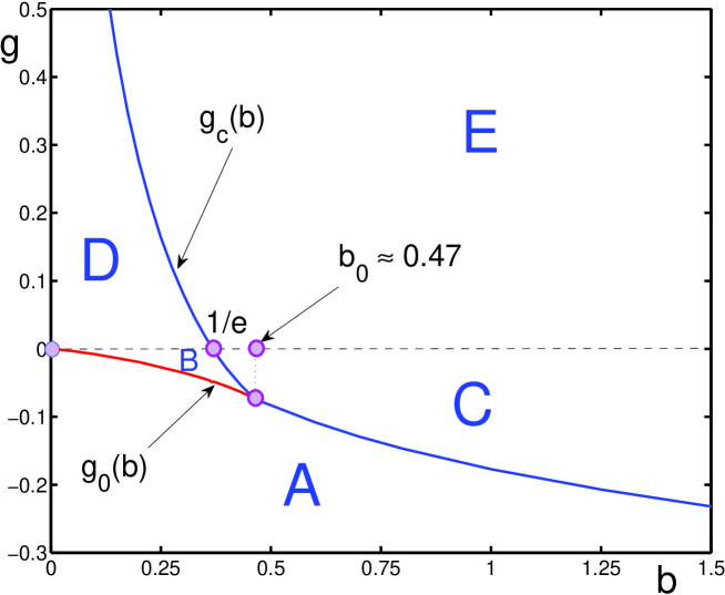
Figure 1: Region of existence of stationary solutions corresponding to the fixed points of the evolution equations for the asset price $x$ and bond price $z$.

The $b$-$g$ plane is partitioned into four regions by the lines $g=0$, $g=g_{0}(b)$, and $g=g_{c}(b)$, as is shown in Fig. 1. The four regions are as follows.

A. When either

$$0<b<b_{0}\;,\qquad g<g_{0}(b)\;,$$ (15)

or

$$b>b_{0}\;,\qquad g<g_{c}(b)\;,$$ (16)

there exists a single fixed point $\{x_{3}^{*},z_{3}^{*}\}$ that is a stable focus, which degenerates to a stable node in the vicinity of the line $g_{0}(b)$.

B. When either

$$0<b<\frac{1}{e}\;,\qquad g_{0}(b)<g<0\;,$$ (17)

or

$$\frac{1}{e}<b<b_{0}\;,\qquad g_{0}(b)<g<g_{c}(b)\;,$$ (18)

there are three fixed points, an unstable focus $\{x_{1}^{*},z_{1}^{*}\}$, a saddle $\{x_{2}^{*},z_{2}^{*}\}$, and a stable node $\{x_{3}^{*},z_{3}^{*}\}$.

C. For

$$b>\frac{1}{e}\;,\qquad g_{c}(b)<g<0\;,$$ (19)

there is an unstable focus $\{x_{1}^{*},z_{1}^{*}\}$ and there appears a limit cycle around this focus.

D. When

$$0<b<\frac{1}{e}\;,\qquad 0\leq g<g_{c}(b)\;,$$ (20)

there are two fixed points, a saddle $\{x_{2}^{*},z_{2}^{*}\}$ and a stable node $\{x_{3}^{*},z_{3}^{*}\}$.

E. Finally, when either

$$0<b<\frac{1}{e}\;,\qquad g>g_{c}(b)\;,$$ (21)

or

$$b>\frac{1}{e}\;,\qquad g\geq 0\;,$$ (22)

there are no fixed points.

The transformation of fixed points, when moving from one region to another, can be illustrated by the corresponding bifurcation paths.

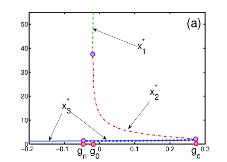
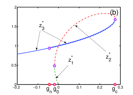
Figure 2: Bifurcation path ${\bf A\longrightarrow B\longrightarrow D\longrightarrow E}$. Here $b=0.2<1/e$ is fixed and $g$ varies: (a) asset price $x^{*}$; (b) bond price $z^{*}$. The fixed point $\{x_{3}^{*},z_{3}^{*}\}$ (solid line) is a stable focus transforming into a stable node (solid line with dots) at $g_{n}\approx-0.0471$. The point exists for $-\infty<g<g_{c}$. The fixed point $\{x_{2}^{*},z_{2}^{*}\}$ (dashed-dotted line) is a saddle, which exists for $g_{0}<g<g_{c}$, and the fixed point $\{x_{1}^{*},z_{1}^{*}\}$ (dashed line) is an unstable focus, which exists for $g_{0}<g<0$. At $g=g_{0}$, the fixed points $\{x_{1}^{*},z_{1}^{*}\}$ and $\{x_{2}^{*},z_{2}^{*}\}$ coincide. At $g=g_{c}$, the fixed points $\{x_{3}^{*},z_{3}^{*}\}$ and $\{x_{2}^{*},z_{2}^{*}\}$ coincide. When $g\rightarrow-0$, then $x_{1}^{*}\rightarrow+\infty$ and $z_{1}^{*}\rightarrow 0$. When $g\rightarrow-\infty$, then $x_{3}^{*}\rightarrow 1$ and $z_{3}^{*}\rightarrow 0$. When $g>g_{c}$, fixed points do not exist.

${\bf A\longrightarrow B\longrightarrow D\longrightarrow E}$: this bifurcation path is shown in Fig. 2, when moving from region $A$, through $B$ and $D$, to region $E$ along the line $b=0.2$, for which $0<b<1/e$. Then $g_{0}(b=0.2)=-0.0194$ and $g_{c}(b=0.2)=0.276$. When the stable focus $\{x_{3}^{*},z_{3}^{*}\}$ in the region $A$ approaches $g_{0}(b)$, it degenerates to a stable node at $g_{n}=-0.0471$ and then survives in the region $B$ where, in addition, there appear an unstable focus $\{x_{1}^{*},z_{1}^{*}\}$ and a saddle $\{x_{2}^{*},z_{2}^{*}\}$. Moving further from the region $B$ to the region $D$, there remain only the stable node $\{x_{3}^{*},z_{3}^{*}\}$ and the saddle $\{x_{2}^{*},z_{2}^{*}\}$. Going from region $D$ to region $E$ by crossing $g_{c}(b)$, all fixed points cease to exist.

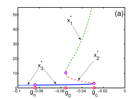
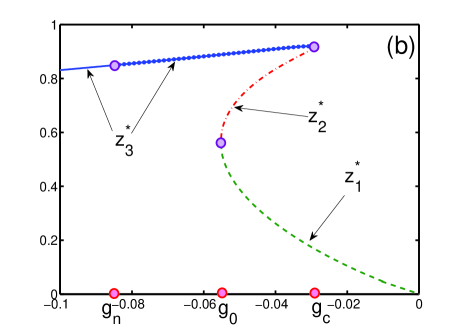
Figure 3: Bifurcation path ${\bf A\longrightarrow B\longrightarrow C\longrightarrow E}$. Here $1/e<b=0.4<b_{0}$ and $g$ varies: (a) asset price $x^{*}$; (b) bond price $z^{*}$. The fixed point $\{x_{3}^{*},z_{3}^{*}\}$ (solid line) is a stable focus transforming to a stable node (solid line with dots) at $g_{n}\approx-0.0849$. The point exists for $-\infty<g<g_{c}<0$. The fixed point $\{x_{2}^{*},z_{2}^{*}\}$ (dashed-dotted line) is a saddle, which exists for $g_{0}<g<g_{c}$, and the fixed point $\{x_{1}^{*},z_{1}^{*}\}$ (dashed line) is an unstable focus, which exists for $g_{0}<g<0$. At $g=g_{0}$, the fixed points $\{x_{1}^{*},z_{1}^{*}\}$ and $\{x_{2}^{*},z_{2}^{*}\}$ coincide. At $g=g_{c}$, the fixed points $\{x_{3}^{*},z_{3}^{*}\}$ and $\{x_{2}^{*},z_{2}^{*}\}$ coincide. When $g\rightarrow-0$, then $x_{1}^{*}\rightarrow+\infty$ and $z_{1}^{*}\rightarrow 0$. When $g\rightarrow-\infty$, then $x_{3}^{*}\rightarrow 1$ and $z_{3}^{*}\rightarrow 0$. When $g\geq 0$, fixed points do not exist.

${\bf A\longrightarrow B\longrightarrow C\longrightarrow E}$: this bifurcation path along the line $b=0.4$, such that $1/e<b<b_{0}=0.47$, is illustrated in Fig. 3. Here $g_{0}(b=0.4)=-0.0552$ and $g_{c}(b=0.4)=-0.0294$. Moving upward in the region $A$, the stable focus $\{x_{3}^{*},z_{3}^{*}\}$ becomes a stable node at $g_{n}=-0.0849$. The stable node $\{x_{3}^{*},z_{3}^{*}\}$ survives into region $B$, where there appear two more fixed points, an unstable focus $\{x_{1}^{*},z_{1}^{*}\}$ and a saddle $\{x_{2}^{*},z_{2}^{*}\}$. In region $C$, the unstable focus $\{x_{1}^{*},z_{1}^{*}\}$ remains and there appears a limit cycle around it. In the region $E$, where $g>0$, there are no fixed points.

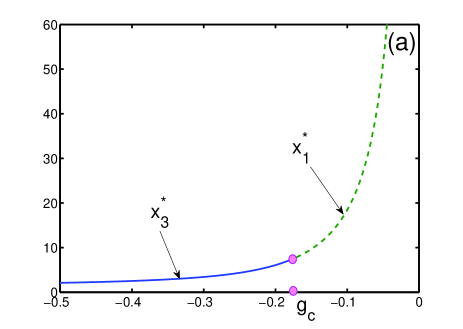
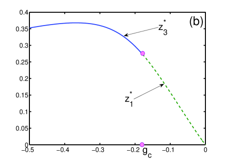
Figure 4: Bifurcation path ${\bf A\longrightarrow C\longrightarrow E}$. Here $b=1>b_{0}$ is fixed and $g$ varies: (a) asset price $x^{*}$; (b) bond price $z^{*}$. The fixed point $\{x_{3}^{*},z_{3}^{*}\}$ (solid line) is a stable focus, and the fixed point $\{x_{1}^{*},z_{1}^{*}\}$ (dashed line) is an unstable focus. At $g=g_{c}\approx-0.1769$, the stable focus transforms into an unstable focus with $x_{3}^{*}=x_{1}^{*}=e^{2}$, $z_{3}^{*}=z_{1}^{*}=2/(be^{2})$, the Lyapunov exponents being ${\Re}\lambda_{1,2}=0$.

${\bf A\longrightarrow C\longrightarrow E}$: the bifurcation path along the line $b=1>b_{0}=0.47$ is given in Fig. 4. Then $g_{c}(b=1)=-0.1769$. The stable focus $\{x_{3}^{*},z_{3}^{*}\}$ in region $A$ transforms in region $C$ into an unstable focus $\{x_{1}^{*},z_{1}^{*}\}$ and there appears a limit cycle. The characteristic exponents at the critical line $g_{c}(b)$ are purely imaginary. No fixed points exist in the region $E$.

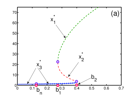
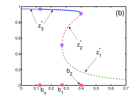
Figure 5: Bifurcation path ${\bf A\longrightarrow B\longrightarrow C}$. Here $g=-0.03$ is fixed and $b$ varies: (a) asset price $x^{*}$; (b) bond price $z^{*}$. The fixed point $\{x_{3}^{*},z_{3}^{*}\}$ (solid line) is a stable focus transforming to a stable node (solid line with dots) at $b_{n}\approx 0.1242$. The point exists for $0\leq b<b_{2}$, where $b_{2}\approx 0.4007$. The fixed point $\{x_{2}^{*},z_{2}^{*}\}$ (dashed-dotted line) is a saddle, which exists for $b_{1}<b<b_{2}$, where $b_{1}\approx 0.2718$. The fixed point $\{x_{1}^{*},z_{1}^{*}\}$ (dashed line) is an unstable focus, which exists for $b>b_{1}$. At $b=b_{1}$, the fixed points $\{x_{1}^{*},z_{1}^{*}\}$ and $\{x_{2}^{*},z_{2}^{*}\}$ coincide. At $b=b_{2}$, the fixed points $\{x_{3}^{*},z_{3}^{*}\}$ and $\{x_{2}^{*},z_{2}^{*}\}$ coincide. When $b=0$, then $x_{3}^{*}=1$ and $z_{3}^{*}=e^{g}$. When $b\rightarrow+\infty$, then $x_{1}^{*}\rightarrow+\infty$ and $z_{1}^{*}\rightarrow 0$.

${\bf A\longrightarrow B\longrightarrow C}$: the bifurcation path along the line $g=-0.03$ is presented in Fig. 5. The critical lines are crossed at the points $b_{1}\equiv b_{0}(g=-0.03)=g_{0}^{-1}(g=-0.03)=0.2718$ and $b_{2}\equiv b_{c}(g=-0.03)=g_{c}^{-1}(g=-0.03)=0.4007$. The stable focus $\{x_{3}^{*},z_{3}^{*}\}$ in region $A$ becomes a stable node at point $b_{n}=0.1242$ that survives into region $B$, where an unstable focus $\{x_{1}^{*},z_{1}^{*}\}$ and a saddle $\{x_{2}^{*},z_{2}^{*}\}$ appear. At the boundary $b_{2}$, the stable node $\{x_{3}^{*},z_{3}^{*}\}$ and a saddle $\{x_{2}^{*},z_{2}^{*}\}$ merge together, while the unstable focus $\{x_{1}^{*},z_{1}^{*}\}$ continues to the region $C$, where a limit cycle arises.

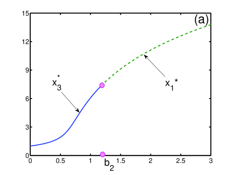
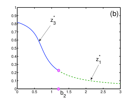
Figure 6: Bifurcation path ${\bf A\longrightarrow C}$. Variation of fixed points under fixed $g=-0.2$ and changing $b$: (a) asset price $x^{*}$; (b) bond price $z^{*}$. The fixed point $\{x_{3}^{*},z_{3}^{*}\}$ (solid line) is a stable focus that at $b=b_{2}\approx 1.1864$ transforms into an unstable focus $\{x_{1}^{*},z_{1}^{*}\}$ (dashed line). At $b=b_{2}$, the fixed points $\{x_{3}^{*},z_{3}^{*}\}$ and $\{x_{1}^{*},z_{1}^{*}\}$ coincide, with the Lyapunov exponents being ${\Re}\lambda_{1,2}=0$.

${\bf A\longrightarrow C}$: the bifurcation path along the line $g=-0.2$ is shown in Fig. 6. The critical line $g_{c}(b)$ is crossed at the point $b_{2}\equiv b_{c}(g=-0.2)=g_{c}^{-1}(g=-0.2)=1.1864$. Here, the stable focus $\{x_{3}^{*},z_{3}^{*}\}$ in region $A$ transforms into an unstable focus $\{x_{1}^{*},z_{1}^{*}\}$ in region $C$, where also a limit cycle appears.

The limit cycle, representing periodically occurring bubbles and crashes in asset prices, appears in two cases. One is the path $A\longrightarrow C$, with crossing the critical line $g_{c}(b)$, accompanied by the bifurcation stable focus $\Longrightarrow$ unstable focus $+$ limit cycle, which is a typical Hopf bifurcation.

The second case happens when crossing the line $g_{c}(b)$ in the path $B\longrightarrow C$, with the bifurcation stable node $+$ saddle $+$ unstable focus $\Longrightarrow$ unstable focus $+$ limit cycle.

4 Periodically collapsing bubbles

4.1 Different types of bubbles

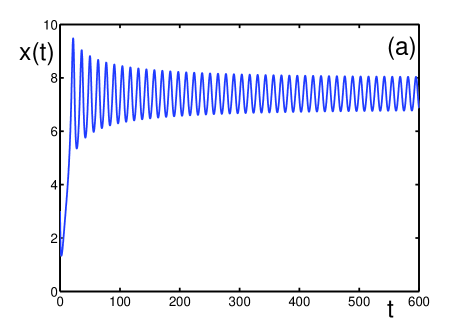
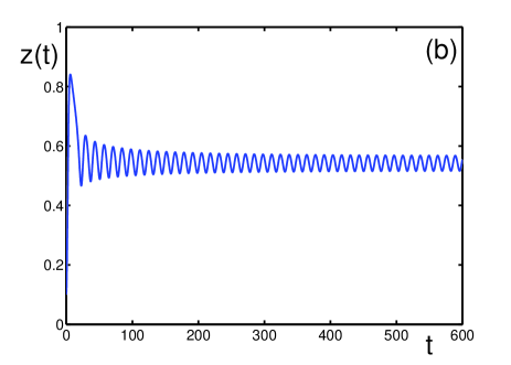
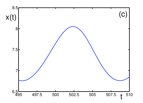
Figure 7: Behavior of the solutions for the asset price and bond price for the parameters $b=0.5$, $g=-0.083$, and the initial conditions $x_{0}=3$ and $z_{0}=0.1$. Here, $g_{c}\approx-0.083056$. (a) Asset price $x(t)$ for $t\in[0,600]$; (b) bond price $z(t)$ for $t\in[0,600]$; (c) a single zoomed out bubble of the asset price $x(t)$ for $t\in[495,510]$; (d) a zoomed out negative bubble of the bond price $z(t)$ for $t\in[495,510]$.

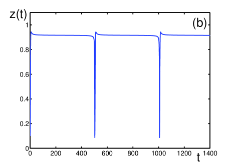
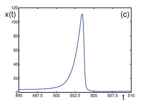
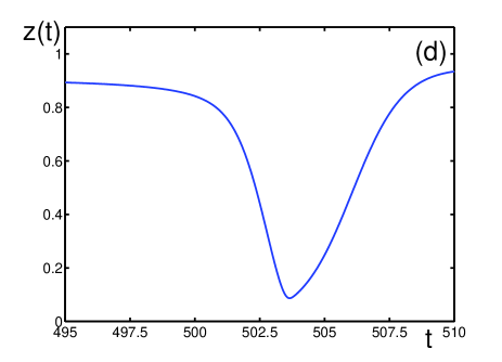
Figure 8: Asset price and bond price for the parameters $b=0.4$, $g=-0.0294$, and the initial conditions $x_{0}=3$ and $z_{0}=0.1$. Here, $g_{c}\approx-0.029424$. (a) Asset price $x(t)$ for $t\in[0,1400]$; (b) bond price $z(t)$ for $t\in[0,1400]$; (c) a zoomed out bubble of the asset price $x(t)$ for $t\in[495,510]$; (d) a zoomed out negative bubble of the bond price $z(t)$ for $t\in[495,510]$.

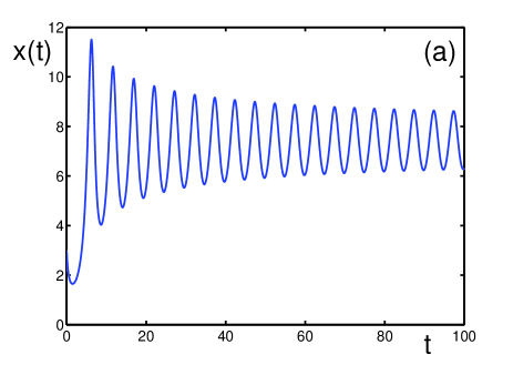
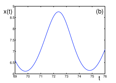
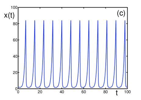
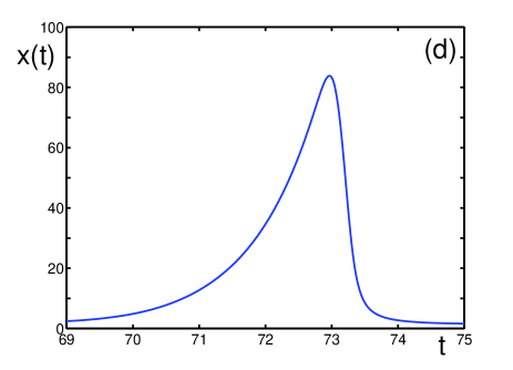
Figure 9: Change in the behavior of the asset price $x(t)$, with the initial conditions $x_{0}=3$, $z_{0}=0.1$, parameters $b=1$, and varying $g$: (a) $g=-0.176>g_{c}$, where $g_{c}(b)=-0.176862964$. The asset price $x(t)$ oscillates without convergence as $t\rightarrow\infty$; (b) a bubble of $x(t)$ for $t\in[69,75]$, with the same parameters as in (a); (c) $g=-0.05$. The asset price $x(t)$ displays periodic bubbles and crashes, as $t\rightarrow\infty$. (d) a bubble of the asset price $x(t)$ for $t\in[69,75]$, under the same parameters as in (c).

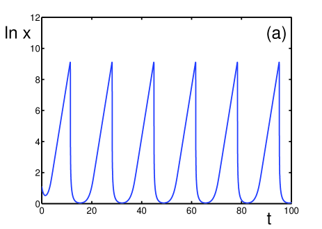
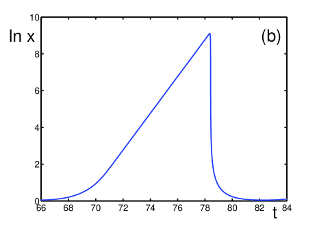
Figure 10: Logarithmic behavior of the asset price for the parameters $b=1$, $g=-0.001$, and the initial conditions $x_{0}=3$ and $z_{0}=0.1$. (a) The function $\ln x(t)$ oscillates without convergence for $t\rightarrow\infty$; (b) a bubble of $\ln x(t)$ for $t\in[66,84]$ under the same parameters as in (a).

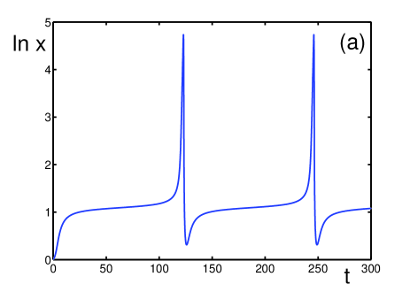
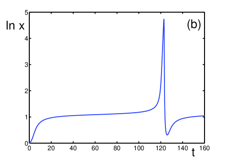
Figure 11: Logarithmic behavior of the asset price $x(t)$ for the parameters $b=0.4$, $g=-0.029$, and the initial conditions $x_{0}=1$ and $z_{0}=0.1$. Here, $g_{c}(b)=-0.029424$. (a) The function $\ln x(t)$ oscillates without convergence as $t\rightarrow\infty$; (b) a bubble of $\ln x(t)$ for $t\in[0,160]$, with the same parameters as in (a).

We find periodically sharply increasing and fast decreasing prices in region $C$. The amplitude, periodicity, as well as the shape of the price trajectories depend on the parameters $b$ and $g$. Figure 7 shows the behavior of the asset price $x(t)$ and bond prices z(t), where $x(t)$ and $z(t)$ are out of phase: an increase in the asset price is accompanied by a decrease in the bond price and vice-versa. In this parameter regime, the price rise and decay are symmetric, representing a typical business cycle regime. In contrast, Fig. 8 shows a parametrization, for which the price of the asset is exhibiting a bubble-like trajectory followed by a sharp faster correction. The prices remain periodic and the structure is that of periodically collapsing bubbles. We find that the asymmetry increases when $g$ approaches the line $g=0$, as is demonstrated in Fig. 9. The distance between the bubbles increases when approaching the line $g_{c}(b)$ with $1/e<b<b_{0}$, as illustrated in Figs. 10 and 11.

We find that the maximum of the asset price $x(t_{max})$ occurs at a time $t_{max}$ that always precedes the time $t_{min}^{z}$, where the bond price $z(t_{min}^{z})$ has its minimum. The time lag $\Delta t\equiv t_{min}^{z}-t_{max}$ depends on the parameters $b$ and $g$. Rather than considering the absolute value of $\Delta t$, we quantify its relative value reduced to the bubble width $w$ measured at the half amplitude of the corresponding bubble. Varying the parameters $b$ and $g$ inside the region $C$, we find that the relative asset-bond time lag $(\Delta t/w)\times 100\%$ is of order $10\%$.

An economic interpretation is as follows. The price rise during a bubble reflects an exuberant market that anticipates a booming economy. Two mechanisms concur to drive the bond prices lower, and thus the interest rate higher. As the economy is booming, it needs investment for growth. There is thus a scarcity of money, which makes its cost larger. In other words, the cost of credit increases and the interest rates rise. At the macro level, the central bank is also often tempted to moderate the exuberance of the bubble by making more expensive the access to credit, thus increasing the short-term interest rate that it can control. The fact, that the maximum of the asset price $x(t_{max})$ occurs at a time $t_{max}$ that always precedes the time $t_{min}^{z}$, where the bond price $z(t_{min}^{z})$ has its minimum, means that the credit dynamics and/or central bank intervention lags behind the price dynamics. This is in agreement with detailed analyses that have shown that stock markets in the US in general lead the Fed rate interventions [43, 44]. If we consider that the dotcom bubble developed from Jan. 1997 to March 2000, covering roughly 39 months, the relative lag of 10% we find in our model translates into about 4 months calendar time, which is in agreement with the estimation of the lag of about a quarter [43, 44].

4.2 Least stable phase during bubbles

As seen in Figs. 8-11, the rising part of a bubble phase is characterized by a fast acceleration, which will be quantified precisely below. Given this strong growth regime, one can expect the prices to be more and more susceptible to external influences and shocks. Does the maximum susceptibility occur during the bubble ascent, at its maximum, or later during the crash?

In the case of a strong asymmetry between the bubble ascent phase and the sharp crash correction, it is tempting to use an analogy with phase transitions and critical phenomena, where the point of phase transitions would correspond to the asset price peak. Then, one could expect that the response functions [45] would be maximal at the points of phase transitions, where the system is supposed to be unstable [46, 47]. But our dynamical system is globally stable as a result of the feedback loops between the asset and bond prices. This translates into a globally stable periodic attractor, notwithstanding the very nonlinear nature of the oscillations, which we have termed “periodically collapsing bubbles” on reference to their shapes. Thus, the correct way to quantify the susceptibility is via a local stability measure called the relative expansion exponent [48, 49], defined as the sum of the local Lyapunov exponents: the larger the expansion exponent, the lower the system stability.

For the dynamical system (10), the local expansion exponent is defined as [48, 49]

$$\Lambda\equiv\frac{1}{t}\int_{0}^{t}{\rm Tr}\hat{J}(x(t^{\prime}),z(t^{\prime}))\;dt^{\prime}\;,$$ (23)

where $\hat{J}(x,z)$ is the Jacobian matrix

$$\hat{J}(x,z)=\left[\begin{array}[]{cc}\frac{\partial f_{1}}{\partial x}&~{}~{}\frac{\partial f_{1}}{\partial z}\\ \\ \frac{\partial f_{2}}{\partial x}&~{}~{}\frac{\partial f_{2}}{\partial z}\end{array}\right]$$ (27)

for the dynamical system (10) with

$$f_{1}:=x-x^{2}e^{-bxz}\;,f_{2}:=z-z^{2}e^{-gx}\;.$$

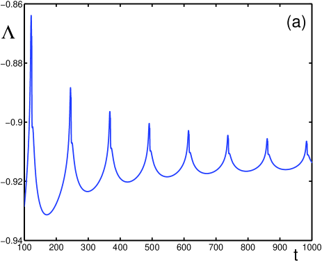
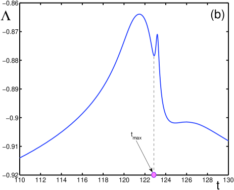
Figure 12: Expansion exponent $\Lambda(t)$, with the parameters $b=0.4$, $g=-0.029$, and the initial conditions $x_{0}=1$ and $z_{0}=0.1$, for different temporal scales: (a) $t\in[100,1000]$; (b) $t\in[110,130]$. At $t_{max}\approx 122.89$, the asset price $x(t)$ has its first local maximum $x_{max}=61.7171$, which corresponds to the first local minimum of $\Lambda(t)$.

Numerical investigation shows that the expansion exponent $\Lambda$ is always negative, which confirms that the dynamical system is always stable in the sense that the dynamics remains bounded and non-chaotic. The largest value of $\Lambda$ corresponds to the least stable state. It turns out that the market, described by the system of Eqs. (10), is the least stable not where the asset price reaches its maximal value. This is illustrated in Fig. 12 for the same parameters ($b=0.4$ and $g=-0.029$) used in Fig. 11. The asset price reaches its first maximum $x(t_{max})=61.717$ at $t_{max}=122.89$, where the expansion exponent presents a local minimum $\Lambda(t_{max})=-0.878$. The algebraic maximum of the expansion exponent $\Lambda(t_{\Lambda})=-0.864$ occurs at the time $t_{\Lambda}=121.48$, which is slightly earlier than $t_{max}$. Thus, the asset price is the least stable not at its maximum but just before it.

4.3 Quantification of exploding bubbles

We have found that the asset price $x(t)$ can be well approximated during the bubble explosion by the following analytical form

$$x_{app}(t)=\frac{c_{1}}{(t_{\Lambda}-t)^{\beta}}\;\exp\left\{\frac{c_{2}}{(t_{\Lambda}-t)^{\alpha}}\right\}\;,$$ (28)

where $t_{\Lambda}$ is the point of maximum of the expansion exponent $\Lambda(t)$.

Our numerical investigations lead us to conclude that the exponents $\alpha$ and $\beta$, for the values of $b$ and $g$ in the left corner of the region $C$, between region $B$ and $E$, where $1/e<b<b_{0}$ and $g>g_{c}(b)$, are close to

$$\alpha=\frac{2}{5}\;,\qquad\beta=\frac{1}{5}~{}.$$ (29)

The numerical coefficients $c_{1}$ and $c_{2}$ are positive parameters that depend on the specific values of $b$ and $g$. For instance, for $b=0.4$ and $g=-0.029$, we have $c_{1}=2.8$, $c_{2}=1.5$, and $t_{\Lambda}=121.48$.

It is interesting to find out whether there exists a critical region where the parameters $\alpha$ and $\beta$ are invariant, being close to $\alpha=0.4$ and $\beta=0.2$, respectively. We have accomplished a detailed analysis over the whole region $C$. It turned out that approximation (28) describes very well the transitional behavior of the beginning of the bubble bursting for the parameters $b$ and $g$ in the vicinity of the double critical point $\{b=1/e,\;g=0\}$, which is the intersection point of the critical lines $b=b_{c}(g)$ and $g=0$, where the exponents $\alpha$ and $\beta$ play the role of a kind of critical indices.

Moreover, the super-exponential form of the initial stage of bursting bubbles is well represented by approximation (28) in a finite region of the parameters $b$ and $g$ corresponding to the triangle, where $1/e<b<b_{0}$ and $g>g_{c}(b)$. In this critical region, the exponents $\alpha$ and $\beta$ are invariant, and only the parameters $c_{1}$ and $c_{2}$ have to be adjusted. For example, let us take $b=0.38$ and $g=-0.0117$, for which $g_{c}=-0.01174$. Then the asset price reaches its first maximum $x(t_{max})=393.5$ at $t_{max}\approx 501.5$, where the expansion exponent possesses its local minimum $\Lambda(t_{max})=-0.9607$, while the absolute maximum of the expansion exponent $\Lambda(t_{\Lambda})=-0.9535$ occurs at the time $t_{\Lambda}\approx 499.74<t_{max}$. Then the critical exponents $\alpha=0.4$ and $\beta=0.2$ can be kept invariant, and only the parameters $c_{1}\approx 1.5$ and $c_{2}\approx 2.8$ are varied.

In order to give a deeper understanding justifying why and where the super-exponential form (28) serves as a good description of the transition from a smooth, almost unchangeable, behavior of the asset price to the start of a bursting bubble, let us study the ratio $R=width/period$ defined as the ratio of the temporal bubble width, measured at half of its amplitude, to the temporal period between the bubbles. It is reasonable to expect that, for genuine bubbles, the ratio $R$ has to be small, representing sharp bubble bursts and crashes interspersed within a smooth market behavior. Our numerical investigation shows that the super-exponential form (28), with invariant exponents $\alpha=0.4$ and $\beta=0.2$, is valid as long as $R\ll 1$, which occurs in the triangle region where $1/e<b<b_{0}\approx 0.47$ and $g_{c}<g<0$.

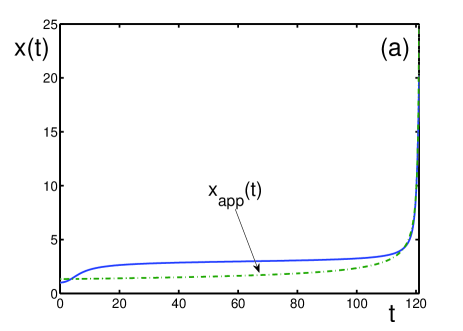
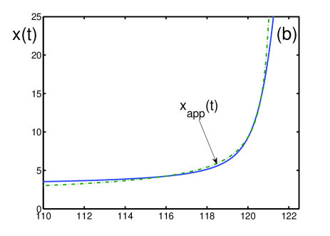
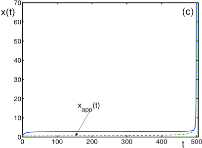
Figure 13: Comparison of the numerical solution for the asset price $x(t)$ (solid line) and its approximation $x_{app}(t)$ (dashed-dotted line), with initial conditions $x_{0}=1$ and $z_{0}=0.1$, for different parameters $b$ and $g$, where $1/e<b<b_{0}\approx 0.47$, and for different intervals of time: (a) $b=0.4$, $g=-0.029>g_{c}=-0.02943$, and $t\in[0,121]$; (b) $b$ and $g$, as in Fig. 13a, but $t\in[110,121]$; (c) $b=0.38$, $g=-0.0117>g_{c}=-0.01174$, and $t\in[0,499.6]$; (d) $b$ and $g$, as in Fig. 13c, but $t\in[489,499.6]$;

The super-exponential behavior (28) is reminiscent of the many reported empirical cases of financial bubbles [3, 50, 51, 52, 53, 54], whose structure can serve as a precursor of the appearing bubble [28]. We note that the transient super-exponential explosive bubble trajectory is here stronger than the simple power law singularities discussed elsewhere [52, 53, 54] as form (28) represents an intermediate asymptotic with an essential singularity behavior. Figure 13 demonstrates the excellent accuracy of the approximation (28), as compared to the accurate “exact” numerical solution $x(t)$ in the region of its accelerated growth.

4.4 Period and amplitude of the periodically collapsing bubbles

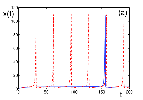
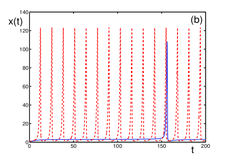
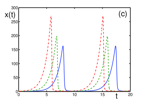
Figure 14: Change in the behavior of the asset price $x(t)$, with fixed $g=-0.03$, when varying $b$ in the vicinity of the boundary point $b_{2}=0.400691$ separating the regions with different numbers of fixed points. The initial conditions are $x_{0}=1$ and $z_{0}=0.1$. (a) Asset price $x(t)$ for $b=0.401>b_{2}$ (solid line) and for $b=0.41$ (dashed-dotted line) for $t\in[0,200]$; (b) asset price $x(t)$ for $b=0.401>b_{2}$ (solid line) and for $b=0.501$ (dashed-dotted line) for $t\in[0,200]$; (c) asset price $x(t)$ for $b=1$ (solid line), for $b=2$ (dashed line), and for $b=10$ (dashed-dotted line), with $t\in[0,20]$.

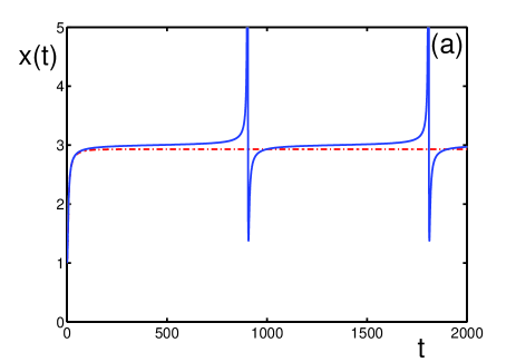
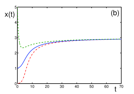
Figure 15: Asset price $x(t)$ for the parameter $g=-0.03$, but with different $b$ and for different initial conditions $\{x_{0},z_{0}\}$. (a) Asset price $x(t)$ for $b=0.4007>b_{2}$ (solid line), $b=0.4006<b_{2}$ (dashed-dotted line), and the initial conditions $x_{0}=1$ and $z_{0}=0.1$. Here, $b_{2}=0.400691$ is the boundary point, such that for $b>b_{2}$, there is an unstable focus and a limit cycle, while for $b<b_{2}$, there are three fixed points. The fixed point $\{x_{3}=2.928,z_{1}=0.916\}$ is a stable node, with the Lyapunov exponents $\{\lambda_{1}=-0.903,\lambda_{2}=-0.022\}$. The fixed point $\{x_{2}=3.08,z_{2}=0.912\}$ is a saddle, with the Lyapunov exponents $\{\lambda_{1}=-0.899,\lambda_{2}=+0.022\}$, and the fixed point $\{x_{1}=58.26,z_{1}=0.174\}$ is an unstable focus, with the Lyapunov exponents $\{\lambda_{1}=\lambda_{2}^{*}=+1.03-i1.72\}$. (b) Asset price $x(t)$ for the parameters $g=-0.03$, $b=0.4007>b_{2}$, and different initial conditions: $\{x_{0}=1,z_{0}=0.1\}$ (solid line), $\{x_{0}=5,z_{0}=0.5\}$ (dashed line), and $\{x_{0}=0.01,z_{0}=50\}$ (dashed-dotted line).

The shape of the bubbles and the distance between them strongly depends on the closeness of the parameters to the critical lines $g=g_{c}(b)$ and $g=0$. This results from the existence of a stable node in the region $B$, which influences the length of the plateaus between the bubbles in the region $C$, as is seen in Figs. 8 and 11. Increasing the distance from the boundary, separating the regions $B$ and $C$, that is, increasing $b$ with fixed $g$, shortens the plateau length between two successive bubbles, but does not influence much the bubble amplitude. This is illustrated in Fig. 14. The level of the plateaus does not depend on initial conditions, as is demonstrated in Fig. 15.

The boundary $g_{c}(b)$ plays the role of a critical line at which the plateau length diverges, similarly to the divergence of the correlation length of statistical physics systems at a phase transition line [46, 47]. To describe this divergence, let us define the duration

$$L\equiv t_{n+1}-t_{n}$$ (30)

between two successive maxima of the asset price $x(t_{n})$ occurring at the times $t_{n}$ and $t_{n+1}$. In other words, $L$ is the time interval between two successive bubbles. This interval, for a fixed $g$, essentially depends on the deviation

$$\Delta\equiv b-b_{c}(g)$$ (31)

of $b$ from the boundary point $b_{c}(g)\equiv g_{c}^{-1}(g)$. The critical behavior can be characterized by the power law

$$L=L(\Delta)\propto\Delta^{-\nu}\qquad(\Delta\rightarrow+0)\;.$$ (32)

Hence, the critical index is given by the limit

$$\nu=-\lim_{\Delta\rightarrow+0}\;\frac{d\ln L}{d\ln|\Delta|}\;.$$ (33)

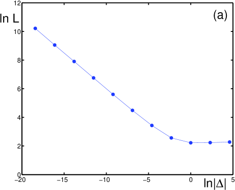
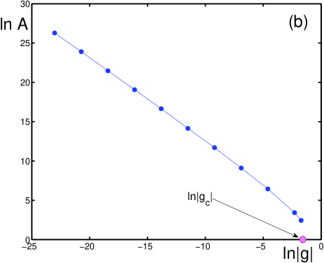
Figure 16: Critical behavior of bubble characteristics. The temporal interval between two neighboring bubbles is $L$. The bubble amplitude is $A$. The distance from the critical line is $\Delta=b-b_{2}$ in (a) and $g$ in (b). The initial conditions are taken as $x_{0}=1$ and $z_{0}=0.1$. (a) Interval $L$ in logarithmic units, as a function of log-distance $\ln|\Delta|=\ln|b-b_{2}|$ to the critical line. Here, $g=-0.03$ and $b_{2}=0.400691$. (b) Bubble amplitude $A$ in logarithmic units, as a function of $\ln|g|$ measuring the distance from the critical line $g=-0$, with fixed $b=1$. Here $g_{c}=-0.1769$, so that $\ln g_{c}=-1.7322$.

Figure 16a shows the behavior of $\ln L$ as a function of $\Delta$, from where we determine $\nu=0.5$.

The other critical line is $g=0$ at which the bubble amplitudes diverge. Above this line, the behavior of the asset price is exponentially inflating. Approaching the critical line $g=0$ from below, the bubble amplitude $A\equiv x(t_{max})$ diverges, analogously to the behavior of the compressibility in statistical physics systems close to a phase transition line, as

$$A=A(g)\propto g^{-\gamma}\qquad(g\rightarrow 0^{-})\;.$$ (34)

This defines the critical index

$$\gamma=-\lim_{g\rightarrow-0}\;\frac{d\ln A}{d\ln|g|}\;.$$ (35)

The dependence of $\ln A$ versus $\ln|g|$ is shown in Fig. 16b, from which we determine $\gamma=1$. Table 1 illustrates the fast divergence of the bubble amplitude $A$, when decreasing $g$ with fixed $b=1$, the number $N$ of bubbles in the time interval $[0,100]$, and the bubble width $w$ measured at half-amplitude. The bubble width, as $g\rightarrow-0$, saturates to $0.7$, while its amplitude diverges.

5 Concluding remarks

We have identified a specific structure of feedback loops between asset prices and bond prices that lead to the regimes of periodically explosive bubbles followed by crashes. While asset and bond prices tend to mean revert to their respective fundamental prices, we have argued that the later are not fixed but depend themselves on the state of the economy represented by the instantaneous asset and bond prices. This results in a rich nonlinear coupled dynamics of asset and bond prices. The two key parameters $b$ and $g$ represent respectively the sensitivity of the fundamental asset price on past asset and bond prices and of the fundamental bond price on past asset prices. They thus capture the competition of the allocation of capital between assets and bonds that develops as the two exhibit diverging trajectories. We stress that the regime of periodically collapsing bubbles does not require heterogeneous agents or sudden changes in market characteristics. Periodically occurring bubbles and crashes can be treated as natural phenomena objectively arising in stock markets due to the delay of the impact of present valuations on future fundamental prices and the nonlinear couplings.

The coupled nonlinear equations (10) have been motivated as the description of the dynamics of a representative asset price coupled with a bond price. There are other possible interpretations. For instance, we can think of the variable $x(t)$ as the monetary base of an economy and $z(t)$ as the spread (or difference) between the yield (interest rate) of bonds with long term maturity (say 10 years) and the interest rate of bonds with short term maturity (say 3 months). The spread $z(t)$ provides a measure of the market expectation on the growth potential of the economy. The larger $z(t)$, the larger the expected growth rate. When $x$ is increasing and $z$ is large, this means that short-term interest rates are low (cheap funding and borrowing) and long term interest rates are increasing (expectation of a growing economy with growing returns). This boosts the monetary base on the anticipation of a growing economy and as a result of the growth of the economy that needs financing. This is the mechanism by which a larger $z$ promotes a future larger monetary base $x$. The multiplicative nature of the equations (10) capture the fact that the positive effect of $z$ on $x$ is all the larger, the larger are $x$ and $z$. But as the monetary base $x$ increases, it generally grows faster than the real economy, leading to misallocation of funding to non-performing industry sectors. This then tends to push $z$ down, on the expectation that long-term interest rates will become smaller as a result of the slowing down of the economy. Also, the economy in its boom phase is over heating and usually requires the intervention of the monetary authorities, who are led to increase the short term interest rates (the cost of short-term borrowing) to stabilize the economy. The larger $x$, the more negative its impact on $z$, hence on its limiting fundamental value. This is captured by the dynamic equations (10). Thus, the regimes of parameters in region $C$, that we have reported in this article, demonstrate the difficulties in stabilizing an economy with the usual monetary tools consisting in attempt to control the monetary base and the interest rates. Due to intrinsic delay and nonlinear feedbacks, such attempts can lead to unintended cycles of booms and busts, as documented for the period from 1980 to present and its role in the great crisis of 2008, following great recession and on-going global crises [55].

Figure captions

Figure 1. Region of existence of stationary solutions corresponding to the fixed points of the evolution equations (10) for the asset price $x$ and bond price $z$.

Figure 2. Bifurcation path ${\bf A\longrightarrow B\longrightarrow D\longrightarrow E}$. Here $b=0.2<1/e$ is fixed and $g$ varies: (a) asset price $x^{*}$; (b) bond price $z^{*}$. The fixed point $\{x_{3}^{*},z_{3}^{*}\}$ (solid line) is a stable focus transforming into a stable node (solid line with dots) at $g_{n}\approx-0.0471$. The point exists for $-\infty<g<g_{c}$. The fixed point $\{x_{2}^{*},z_{2}^{*}\}$ (dashed-dotted line) is a saddle, which exists for $g_{0}<g<g_{c}$, and the fixed point $\{x_{1}^{*},z_{1}^{*}\}$ (dashed line) is an unstable focus, which exists for $g_{0}<g<0$. At $g=g_{0}$, the fixed points $\{x_{1}^{*},z_{1}^{*}\}$ and $\{x_{2}^{*},z_{2}^{*}\}$ coincide. At $g=g_{c}$, the fixed points $\{x_{3}^{*},z_{3}^{*}\}$ and $\{x_{2}^{*},z_{2}^{*}\}$ coincide. When $g\rightarrow-0$, then $x_{1}^{*}\rightarrow+\infty$ and $z_{1}^{*}\rightarrow 0$. When $g\rightarrow-\infty$, then $x_{3}^{*}\rightarrow 1$ and $z_{3}^{*}\rightarrow 0$. When $g>g_{c}$, fixed points do not exist.

Figure 3. Bifurcation path ${\bf A\longrightarrow B\longrightarrow C\longrightarrow E}$. Here $1/e<b=0.4<b_{0}$ and $g$ varies: (a) asset price $x^{*}$; (b) bond price $z^{*}$. The fixed point $\{x_{3}^{*},z_{3}^{*}\}$ (solid line) is a stable focus transforming to a stable node (solid line with dots) at $g_{n}\approx-0.0849$. The point exists for $-\infty<g<g_{c}<0$. The fixed point $\{x_{2}^{*},z_{2}^{*}\}$ (dashed-dotted line) is a saddle, which exists for $g_{0}<g<g_{c}$, and the fixed point $\{x_{1}^{*},z_{1}^{*}\}$ (dashed line) is an unstable focus, which exists for $g_{0}<g<0$. At $g=g_{0}$, the fixed points $\{x_{1}^{*},z_{1}^{*}\}$ and $\{x_{2}^{*},z_{2}^{*}\}$ coincide. At $g=g_{c}$, the fixed points $\{x_{3}^{*},z_{3}^{*}\}$ and $\{x_{2}^{*},z_{2}^{*}\}$ coincide. When $g\rightarrow-0$, then $x_{1}^{*}\rightarrow+\infty$ and $z_{1}^{*}\rightarrow 0$. When $g\rightarrow-\infty$, then $x_{3}^{*}\rightarrow 1$ and $z_{3}^{*}\rightarrow 0$. When $g\geq 0$, fixed points do not exist.

Figure 4. Bifurcation path ${\bf A\longrightarrow C\longrightarrow E}$. Here $b=1>b_{0}$ is fixed and $g$ varies: (a) asset price $x^{*}$; (b) bond price $z^{*}$. The fixed point $\{x_{3}^{*},z_{3}^{*}\}$ (solid line) is a stable focus, and the fixed point $\{x_{1}^{*},z_{1}^{*}\}$ (dashed line) is an unstable focus. At $g=g_{c}\approx-0.1769$, the stable focus transforms into an unstable focus with $x_{3}^{*}=x_{1}^{*}=e^{2}$, $z_{3}^{*}=z_{1}^{*}=2/(be^{2})$, the Lyapunov exponents being ${\Re}\lambda_{1,2}=0$.

Figure 5. Bifurcation path ${\bf A\longrightarrow B\longrightarrow C}$. Here $g=-0.03$ is fixed and $b$ varies: (a) asset price $x^{*}$; (b) bond price $z^{*}$. The fixed point $\{x_{3}^{*},z_{3}^{*}\}$ (solid line) is a stable focus transforming to a stable node (solid line with dots) at $b_{n}\approx 0.1242$. The point exists for $0\leq b<b_{2}$, where $b_{2}\approx 0.4007$. The fixed point $\{x_{2}^{*},z_{2}^{*}\}$ (dashed-dotted line) is a saddle, which exists for $b_{1}<b<b_{2}$, where $b_{1}\approx 0.2718$. The fixed point $\{x_{1}^{*},z_{1}^{*}\}$ (dashed line) is an unstable focus, which exists for $b>b_{1}$. At $b=b_{1}$, the fixed points $\{x_{1}^{*},z_{1}^{*}\}$ and $\{x_{2}^{*},z_{2}^{*}\}$ coincide. At $b=b_{2}$, the fixed points $\{x_{3}^{*},z_{3}^{*}\}$ and $\{x_{2}^{*},z_{2}^{*}\}$ coincide. When $b=0$, then $x_{3}^{*}=1$ and $z_{3}^{*}=e^{g}$. When $b\rightarrow+\infty$, then $x_{1}^{*}\rightarrow+\infty$ and $z_{1}^{*}\rightarrow 0$.

Figure 6. Bifurcation path ${\bf A\longrightarrow C}$. Variation of fixed points under fixed $g=-0.2$ and changing $b$: (a) asset price $x^{*}$; (b) bond price $z^{*}$. The fixed point $\{x_{3}^{*},z_{3}^{*}\}$ (solid line) is a stable focus that at $b=b_{2}\approx 1.1864$ transforms into an unstable focus $\{x_{1}^{*},z_{1}^{*}\}$ (dashed line). At $b=b_{2}$, the fixed points $\{x_{3}^{*},z_{3}^{*}\}$ and $\{x_{1}^{*},z_{1}^{*}\}$ coincide, with the Lyapunov exponents being ${\Re}\lambda_{1,2}=0$.

Figure 7. Behavior of the solutions for the asset price and bond price for the parameters $b=0.5$, $g=-0.083$, and the initial conditions $x_{0}=3$ and $z_{0}=0.1$. Here, $g_{c}\approx-0.083056$. (a) Asset price $x(t)$ for $t\in[0,600]$; (b) bond price $z(t)$ for $t\in[0,600]$; (c) a single zoomed out bubble of the asset price $x(t)$ for $t\in[495,510]$; (d) a zoomed out negative bubble of the bond price $z(t)$ for $t\in[495,510]$.

Figure 8. Asset price and bond price for the parameters $b=0.4$, $g=-0.0294$, and the initial conditions $x_{0}=3$ and $z_{0}=0.1$. Here, $g_{c}\approx-0.029424$. (a) Asset price $x(t)$ for $t\in[0,1400]$; (b) bond price $z(t)$ for $t\in[0,1400]$; (c) a zoomed out bubble of the asset price $x(t)$ for $t\in[495,510]$; (d) a zoomed out negative bubble of the bond price $z(t)$ for $t\in[495,510]$.

Figure 9. Change in the behavior of the asset price $x(t)$, with the initial conditions $x_{0}=3$, $z_{0}=0.1$, parameters $b=1$, and varying $g$: (a) $g=-0.176>g_{c}$, where $g_{c}(b)=-0.176862964$. The asset price $x(t)$ oscillates without convergence as $t\rightarrow\infty$; (b) a bubble of $x(t)$ for $t\in[69,75]$, with the same parameters as in (a); (c) $g=-0.05$. The asset price $x(t)$ displays periodic bubbles and crashes, as $t\rightarrow\infty$. (d) a bubble of the asset price $x(t)$ for $t\in[69,75]$, under the same parameters as in (c).

Figure 10. Logarithmic behavior of the asset price for the parameters $b=1$, $g=-0.001$, and the initial conditions $x_{0}=3$ and $z_{0}=0.1$. (a) The function $\ln x(t)$ oscillates without convergence for $t\rightarrow\infty$; (b) a bubble of $\ln x(t)$ for $t\in[66,84]$ under the same parameters as in (a).

Figure 11. Logarithmic behavior of the asset price $x(t)$ for the parameters $b=0.4$, $g=-0.029$, and the initial conditions $x_{0}=1$ and $z_{0}=0.1$. Here, $g_{c}(b)=-0.029424$. (a) The function $\ln x(t)$ oscillates without convergence as $t\rightarrow\infty$; (b) a bubble of $\ln x(t)$ for $t\in[0,160]$, with the same parameters as in (a).

Figure 12. Expansion exponent $\Lambda(t)$, with the parameters $b=0.4$, $g=-0.029$, and the initial conditions $x_{0}=1$ and $z_{0}=0.1$, for different temporal scales: (a) $t\in[100,1000]$; (b) $t\in[110,130]$. At $t_{max}\approx 122.89$, the asset price $x(t)$ has its first local maximum $x_{max}=61.7171$, which corresponds to the first local minimum of $\Lambda(t)$.

Figure 13. Comparison of the numerical solution for the asset price $x(t)$ (solid line) and its approximation $x_{app}(t)$ (dashed-dotted line), with initial conditions $x_{0}=1$ and $z_{0}=0.1$, for different parameters $b$ and $g$, where $1/e<b<b_{0}\approx 0.47$, and for different intervals of time: (a) $b=0.4$, $g=-0.029>g_{c}=-0.02943$, and $t\in[0,121]$; (b) $b$ and $g$, as in Fig. 13a, but $t\in[110,121]$; (c) $b=0.38$, $g=-0.0117>g_{c}=-0.01174$, and $t\in[0,499.6]$; (d) $b$ and $g$, as in Fig. 13c, but $t\in[489,499.6]$;

Figure 14. Change in the behavior of the asset price $x(t)$, with fixed $g=-0.03$, when varying $b$ in the vicinity of the boundary point $b_{2}=0.400691$ separating the regions with different numbers of fixed points. The initial conditions are $x_{0}=1$ and $z_{0}=0.1$. (a) Asset price $x(t)$ for $b=0.401>b_{2}$ (solid line) and for $b=0.41$ (dashed-dotted line) for $t\in[0,200]$; (b) asset price $x(t)$ for $b=0.401>b_{2}$ (solid line) and for $b=0.501$ (dashed-dotted line) for $t\in[0,200]$; (c) asset price $x(t)$ for $b=1$ (solid line), for $b=2$ (dashed line), and for $b=10$ (dashed-dotted line), with $t\in[0,20]$.

Figure 15. Asset price $x(t)$ for the parameter $g=-0.03$, but with different $b$ and for different initial conditions $\{x_{0},z_{0}\}$. (a) Asset price $x(t)$ for $b=0.4007>b_{2}$ (solid line), $b=0.4006<b_{2}$ (dashed-dotted line), and the initial conditions $x_{0}=1$ and $z_{0}=0.1$. Here, $b_{2}=0.400691$ is the boundary point, such that for $b>b_{2}$, there is an unstable focus and a limit cycle, while for $b<b_{2}$, there are three fixed points. The fixed point $\{x_{3}=2.928,z_{1}=0.916\}$ is a stable node, with the Lyapunov exponents $\{\lambda_{1}=-0.903,\lambda_{2}=-0.022\}$. The fixed point $\{x_{2}=3.08,z_{2}=0.912\}$ is a saddle, with the Lyapunov exponents $\{\lambda_{1}=-0.899,\lambda_{2}=+0.022\}$, and the fixed point $\{x_{1}=58.26,z_{1}=0.174\}$ is an unstable focus, with the Lyapunov exponents $\{\lambda_{1}=\lambda_{2}^{*}=+1.03-i1.72\}$. (b) Asset price $x(t)$ for the parameters $g=-0.03$, $b=0.4007>b_{2}$, and different initial conditions: $\{x_{0}=1,z_{0}=0.1\}$ (solid line), $\{x_{0}=5,z_{0}=0.5\}$ (dashed line), and $\{x_{0}=0.01,z_{0}=50\}$ (dashed-dotted line).

Figure 16. Critical behavior of bubble characteristics. The temporal interval between two neighboring bubbles is $L$. The bubble amplitude is $A$. The distance from the critical line is $\Delta=b-b_{2}$ in (a) and $g$ in (b). The initial conditions are taken as $x_{0}=1$ and $z_{0}=0.1$. (a) Interval $L$ in logarithmic units, as a function of log-distance $\ln|\Delta|=\ln|b-b_{2}|$ to the critical line. Here, $g=-0.03$ and $b_{2}=0.400691$. (b) Bubble amplitude $A$ in logarithmic units, as a function of $\ln|g|$ measuring the distance from the critical line $g=-0$, with fixed $b=1$. Here $g_{c}=-0.1769$, so that $\ln g_{c}=-1.7322$.

Table 1. Fast divergence of the bubble amplitude $A$, when decreasing $g$, with fixed $b=1$. $N$ is the number of bubbles in the time interval $[0,100]$, and $w$ is the bubble width measured at half-amplitude.

References

- [1] C. Leung, Macroeconomics and housing: a review of the literature. J. Hous. Econ. 13, 249–267 (2004).
- [2] J. Mauldin and J. Tepper, Code Red: How to Protect Your Savings From the Coming Crisis (Wiley, Berlin, 2013).
- [3] D. Sornette, Why Stock Markets Crash (Princeton University, Princeton, 2003).
- [4] J.M. Keynes, The General Theory of Employment, Interest and Money (Harcourt, New York, 1934).
- [5] C.P. Kindlebeger, Manias, Panics, and Crashes (Basic Books, New York, 1978).
- [6] B. Malkiel, A Random Walk Down Wall Street (Norton, New York, 1985).
- [7] J.K. Galbraith, The Great Crash 1929 (Houghton Mifflin, Boston, 2009).
- [8] T. Lux, Herd behavior, bubbles and crashes. Econ. J. 105, 881–896 (1995).
- [9] D. Sornette and A. Johansen, A hierarchical model of financial crashes. Physica A 261, 581–598 (1998).
- [10] T. Kaizoji, Speculative bubbles and crashes in stock markets. Physica A 287, 493–506 (2000).
- [11] D. Sornette, Physics and financial economics (1776-2014): puzzles, Ising and agent-based models. Rep. Prog. Phys. 77, 062001 (2014).
- [12] P. Krugman, Balance sheets, the transfer problem, and financial crises. Int. Tax Public Financ. 6, 459–472 (1999).
- [13] E. Ozdenoren and K. Yuan, Feedback effects and asset prices. J. Financ. 63, 1939–1975 (2008).
- [14] J. Ganguli and L. Yang, Complimentarities, multiplicity, and supply information. J. Eur. Econ. Assoc. 7, 90–115 (2009).
- [15] U. Cetin and I. Sheynzon, A simple model for market booms and crashes. Math. Finan. Econ. 8, 291–319 (2014).
- [16] D.B. Porter and V.L. Smith, Stock market bubbles in the laboratory. J. Behav. Finan. 4, 7–20 (2003).
- [17] V.I. Yukalov, D. Sornette, and E.P. Yukalova, Nonlinear dynamical model of regime switching between conventions and busines cycles. J. Econ. Behav. Org. 70, 206–230 (2009).
- [18] J. Huang and J. Wang, Liquidity and market crashes. Rev. Finan. Stud. 22, 2607–2643 (2009).
- [19] D. Abreu and M. Brunnermeier, Bubbles and crashes. Econometrica 71, 173–204 (2003).
- [20] J. Scheinkman and W. Xiong, Overconfidence and speculative bubbles. J. Polit. Econ. 111, 1183–1220 (2003).
- [21] F. Allen and D. Gale, Understanding Financial Crises (Clarendon, Oxford, 2009).
- [22] D. Friedman and R. Abraham, Bubbles and crashes: gradient dynamics in financial markets. J. Econ. Dyn. Control 33, 922–937 (2009).
- [23] M. Brunnermeier and M. Oehmke, Bubbles, Financial Crises, and Systemic Risk (North-Holland, Amsterdam, 2012).
- [24] D. Romer, Rational asset-price movements without news. Am. Econ. Rev. 83, 1112–1130 (1993).
- [25] A. Caplin and J. Leahy, Business as usual, market crashes, and a wisdom after the fact. Am. Econ. Rev. 84, 548–565 (1994).
- [26] H. Hong and J. Stein, Differences of opinion, short-scale constraints, and market crashes. Rev. Finan. Stud. 16, 487–525 (2003).
- [27] J. Zeira, Informational overshooting, booms, and crashes. J. Monet. Econ. 43, 237–257 (1999).
- [28] D. Sornette and P. Cauwels, Financial bubbles: mechanisms and diagnostics. Rev. Behav. Econ. (in press) (http://ssrn.com/abstract=2423790).
- [29] K. Wicksell, Interest and Prices (a Study of the Causes Regulating the Value of Money), original publication date 1898, reprinted in (Sentry Press, New York, 1962).
- [30] J.H. Cochrane, Asset Pricing (Princeton University, Princeton, 2001).
- [31] C. Golier, The Economics of Risk and Time (MIT Press, Cambridge, 2001).
- [32] V.I. Yukalov, E.P. Yukalova, and D. Sornette, Modeling symbiosis by interactions through species carrying capacities. Physica D 241, 1270–1289 (2012).
- [33] V.I. Yukalov, E.P. Yukalova, and D. Sornette, Extreme events in population dynamics with functional carrying capacity. Eur. Phys. J. Spec. Top. 205, 313–354 (2012).
- [34] V.I. Yukalov, E.P. Yukalova, and D. Sornette, New approach to modeling symbiosis in biological and social systems. Int. J. Bifur. Chaos 24, 1450117 (2014).
- [35] R. Arditi and L.R. Ginzburg, Coupling in predator-prey dynamics: ratio-dependence. J. Theor. Biol. 139, 311–326 (1989).
- [36] M. Perc and A. Szolnoki, Coevolutionary games - a mini review. Biosystems 99, 109–125 (2010).
- [37] M. Perc, J. Gomez-Gardenes, A. Szolnoki, L.M. Floria, and Y. Moreno, Evolutionary dynamics of group interactions on structural populations: a review. J. Roy. Soc. Interf. 10, 21120997 (2013).
- [38] V.I. Yukalov, Statistical mechanics of strongly nonideal systems. Phys. Rev. A 42, 3324–3334 (1990).
- [39] V.I. Yukalov, Method of self-similar approximations. J. Math. Phys. 32, 1235–1239 (1991).
- [40] V.I. Yukalov, Stability conditions for method of self-similar approximations. J. Math. Phys. 33, 3994–4001 (1992).
- [41] S. Saavedra, R.P. Rohr, L.J. Gilarranz, and J. Bascompte, How stracturally stable are global socioeconomic systems? J. Roy. Soc. Interface 11, 20140693 (2014).
- [42] V.I. Yukalov and S. Gluzman, Self-similar exponential aproximants. Phys. Rev. E 58, 1359–1382 (1998).
- [43] W.-X. Zhou and D. Sornette, Causal slaving of the U.S. treasury bond yield antibubble by the stock market antibubble of August 2000. Physica A 337, 586–608 (2004).
- [44] K. Guo, W.-X. Zhou, S.-W. Cheng, and D. Sornette, The US stock market leads the Federal funds rate and treasury bond yields. PLOS ONE 6, e22794 (2011).
- [45] J. Sieber and J.M. Thompson, Nonlinear softening as a predicitve precursor to climate tipping. Phil. Trans. Roy. Soc. A 370, 1205–1227 (2012).
- [46] V.I. Yukalov, Phase transitions and heterophase fluctuations. Phys. Rep. 208, 395–489 (1991).
- [47] D. Sornette, Critical Phenomena in Natural Sciences (Springer, Berlin, 2006).
- [48] V.I. Yukalov, Principle of pattern selection for nonequilibrium phenomena. Phys. Lett. A 284, 91–98 (2001).
- [49] V.I. Yukalov, Expansion exponents for nonequilibrium systems. Physica A 320, 149–168 (2003).
- [50] W. Yan, R. Rebib, R. Woodard, and D. Sornette, Detection of crashes and rebounds in major equity markets. Int. J. Portfolio Anal. Manag. 1, 59–79 (2012).
- [51] A. Johansen and D. Sornette, Shocks, crashes and bubbles in financial markets. Brussels Econ. Rev. 53, 201–253 (2010).
- [52] Z.Q. Jiang, W.X. Zhou, D. Sornette, R. Woodard, K. Bastiaensen, and P. Cauwels, Bubble diagnosis and prediction of the 2005-2007 and 2008-2009 Chinese stock market bubbles. J. Econ. Behav. Org. 74, 149–162 (2010).
- [53] A. Hüsler, D. Sornette, and C.H. Hommes, Super-exponential bubbles in lab experiments: evidence for anchoring over-optimistic expectations on price. J. Econ. Behav. Org. 92, 304–316 (2013).
- [54] D. Sornette, R. Woodard, W. Yan, and W.X. Zhou, Clarifications to questions and criticisms on the Johansen-Ledoit-Sornette bubble model. Physica A 392, 4417–4428 (2013).
- [55] D. Sornette and P. Cauwels, 1980-2008: The illusion of the perpetual money machine and what it bodes for the future. Risks 2, 103–131 (2014).