A Comparative Analysis of the Successive Lumping and the Lattice Path Counting Algorithms

Abstract

This article provides a comparison of the successive lumping (SL) methodology developed in [19] with the popular lattice path counting [24] in obtaining rate matrices for queueing models, satisfying the specific quasi birth and death structure as in [21], [22]. The two methodologies are compared both in terms of applicability requirements and numerical complexity by analyzing their performance for the same classical queueing models considered in [21]. The main findings are: i) When both methods are applicable the SL based algorithms outperform the lattice path counting  algorithm (LPCA). ii) There are important classes of problems (e.g., models with (level) non-homogenous rates or with finite state spaces) for which the SL methodology is applicable and for which the LPCA cannot be used. iii) Another main advantage of successive lumping algorithms over lattice path counting is that the former includes a method to compute the steady state distribution using this rate matrix.

KATEHAKIS ET AL.

[Rutgers University, NJ, USA]Michael N. Katehakis Department of Management Science and Information Systems, Rutgers University, 100 Rockafeller Road, Piscataway, NJ 08854, USA. E-mail: mnk@rutgers.edu [Leiden University, Netherlands]Laurens C. Smit Mathematisch Instituut, Universiteit Leiden, Niels Bohrweg 1, 2333 CA, The Netherlands, E-mail: lsmit@math.leidenuniv.nl [Leiden University, Netherlands]Floske M. Spieksma Mathematisch Instituut, Universiteit Leiden, Niels Bohrweg 1, 2333 CA, The Netherlands, E-mail: spieksma@math.leidenuniv.nl

60K2568M20

1 Introduction

Two dimensional Markov chains arise as a natural way to model various real life applications. In particular, many queueing models possess this structure and it is even possible that a more complex, higher dimensional queueing model can be decomposed into various two dimensional Markov processes. For various queueing models we refer to [1, 2, 3, 5, 9, 7, 27, 29, 31, 34]. Other areas in which these processes will arise outside queueing are for example inventory models, cf. [18], reliability, cf. [17, 16] and pricing models. In this paper we are particularly interested in a comparison of the new successive lumping (SL) methodology developed in [19] with the popular lattice path counting [24] in obtaining rate matrices for queueing models, as in [22] and [21]. The two methodologies are compared both in terms of applicability requirements and numerical complexity by analyzing their performance for the same classical queueing models considered in [21]. In all these models, the objective is to calculate the steady state distribution of a pertinent Quasi Birth-and-Death (QBD) process (i.e., a two dimensional Markov chain with a transition generator matrix $Q$ that contains nonzero rates only for transitions to the ‘left’ and to the ‘right’ in every state) that describes the evolution of the state of the system in time.

The main method that is used to analyze QBD processes is based on expressing the stationary probabilities of states of one level in terms of those of its previous levels. This is done with the aid of a rate matrix $R$, which is the basis of the matrix-geometric solution introduced by Neuts. For general level-independent QBD processes, it is known that $R$ satisfies a matrix-quadratic equation. Algorithms for solving this equation were given in [26] and Latouche and Ramaswami [20]. A current state of the art software implementing quadratically-convergent algorithms with a number of speed-up features is described in [4]. A general algorithm for the level-independent case can be found in [6] and a discussion of the Quasi Skip Free case in [23].

There are various methods that make use of a special structure of the transition rate matrix $Q$, to provide efficient computation procedures for the rate matrix $R$. Such a procedure is available in the the case in which the ‘down matrix’ of $Q$, is a product of a row and a column vector. For other procedures that explicitly calculate a rate matrix we refer to [30] and [25]. Recent studies, cf. [22, 21], have used lattice path counting  methods to directly compute the rate matrix for certain QBD processes that arise in queueing models. For example, a priority queue model has been analyzed by this method, but also with other techniques, see e.g. [11] and references therein. The idea of counting the number of paths on a lattice, cf. [24, 10], has been used in many fields of applied probability, cf. [28].

A new alternative method to compute the rate matrix for certain QBD processes can be based on the successive lumping (SL) procedure introduced in [14]. It was employed in [19] to obtain explicit solutions for ‘rate sets’ for large classes of QSF processes, the so-called DES and RES processes. The SL approach differs from the previous mentioned works by its distinct method of derivation and its applicability to models with infinite state spaces and models that are outside the QSF framework. However, it should be noted that algorithms given in [11, 20, 6] can be used on other, more general (in terms of down-transitions) processes. The advantages of using SL are described in [19]. Although the nature of a path counting based method and the successive lumping based method are very different, a comparison can be done, since they both rely on the absence of certain kind of transitions. Herein we compare the method introduced in [21] with the one based on successive lumping of [19].

The main contribution of this paper is to provide a clear comparison between successive lumping (SL) based methods and the lattice path counting based algorithm, introduced in [21], in computational complexity and applicability. First, it is shown that the SL methodology yields algorithms that are faster than the counting algorithm. Second, we show that SL based procedures are applicable to many of the queueing models discussed in previous papers, and even to models with finite state spaces or with non-homogenous transition rate structures and to models with a quasi skip free (QSF) structure, cf. [19]. However, there seem to exist some artificial queueing models that do not possess the SL property, for which a lattice path counting algorithm is applicable. Finally, this paper continues the work of [19], and it specializes its results to homogenous QBD processes, in order to make the comparison of successive lumping (SL) based methods and the lattice path counting  procedure possible.

The paper has the following structure. In Section 2 we first define the notation for the QBD processes that we will use throughout the paper. In Section 2 we summarize the results of [19] for the DES processes as they apply to quasi birth and death processes with a down entrance state and the resulting quasi birth and death down entrance state algorithm (QDESA). In Section 2 the QDESA procedure is specialized depending on the structure of the transition rate $Q$, applicable to the models under investigation in this paper. Then, in Section 3 the introduced procedures are clarified by applying them to two specific queueing examples. In Section 4 we review the lattice path counting algorithm. In Section 5 we compare the procedures in speed (computational complexity). In Section 6 we discuss the the type of models for which each procedure can be applied. We conclude with some models that further illustrate these comparisons.

2 Preliminary Results

2.1 Successive Lumping in Quasi Birth and Death Processes

In the sequel we consider an ergodic QBD process $X(t)$ with states in a finite or countable set $\mathcal{X}$. The states (after re-labeling) will be written as tuples $(m,i)$, where in the state description the first entry $m=0,1,\ldots,M$ represents the ‘level’ of the state and the second entry $i=0,1,2,\ldots,\ell_{m}$ represents the ‘stage’ of the state $(m,i)$. The integers $\ell_{m}$ and $M$ are given constants and they represent respectively the number of stages ($\ell_{m}+1$) and the highest level ($M$); these scalars can be infinite. Let $Q$ denote the transition generator matrix. The process $X(t)$ is referred to as a ‘level QBD’ process if the only transitions allowed are to a state that is within the same level or to a level one step above or below, i.e., $Q$ has the form:

$$Q=\left[\begin{array}[]{cccccc}W^{0}&U^{0}&0&\cdots&0&0\\ D^{1}&W^{1}&U^{1}&\ddots&0&0\\ 0&D^{2}&W^{2}&\ddots&0&0\\ \vdots&\ddots&\ddots&\ddots&\vdots&\vdots\\ 0&0&0&\cdots&W^{M-1}&U^{M-1}\\ 0&0&0&\cdots&D^{M}&W^{M}\end{array}\right].$$ (1)

The matrices $W$, $D$ and $U$ represent ‘within a level’, ‘down one level’ and ‘up one level’ transitions respectively. The sub-matrices $W^{m}$ above are of dimension $(\ell_{m}+1)\times(\ell_{m}+1)$, the sub-matrices $D^{m}$ are of dimension $(\ell_{m}+1)\times(\ell_{m-1}+1)$ and the submatrices $U^{m}$ are of dimension $(\ell_{m}+1)\times(\ell_{m+1}+1).$ Further, we will use the notation $\mathcal{L}_{n}=\{(n,i),\ i=0,1,\ldots,\ell\}$ for the level sets ($n=0,1,\ldots,M$).

Let $\pi$ denote the steady state distribution, i.e., the solution of $\pi Q=0$ and $\pi 1=1$. We denote by $\pi^{n}$ the sub-vector of $\pi$ formed by the stationary probabilities of the states of level $n$ i.e., $\pi^{n}=[\,\pi(n,0),\ldots,\pi(n,\ell)\,].$

In the context of the current paper we will assume that every matrix $D^{m}$ has only one nonzero column (that for this section we will assume be the first column). The underlying QBD process is therefore successively lumpable (a DES process) with respect to the partition $\{\mathcal{L}_{n}\}_{n\geq 0}$ of the state space $\mathcal{X}$, cf. [14] for lumping and [19] for a proof that $X(t)$ is lumpable with respect to this partition. In addition we will assume that $\ell_{m}=\ell$ for all $m$ (i.e., the level size is independent of the level) and note that this condition is not necessary for the DES procedure to be applicable, but is necessary for the LPC procedure, that will be discussed in Section 4. Below we will repeat the important definitions from [19], specialized for a QBD process.

In a QBD process we define the matrix $\widetilde{U}^{m}$ of size $(\ell+1)\times(\ell+1)$ as follows:

$$\widetilde{U}^{m}=U^{m}1_{m}^{\prime}\delta_{m},$$ (2)

where $1_{m}$ is a rowvector of size $\ell+1$ with identically equal to $1$ and $\delta_{m}$ is a vector of the same size identically equal to $0$ with a $1$ on its first entry. Furthermore we define:

$$B^{m}=W^{m}+\widetilde{U}^{m}.$$ (3)

For a QBD process, we will call a matrix set $\{\mathcal{R}_{m}\}_{m}$ that satisfies the equation below a rate matrix set.

$$\pi^{m}=\pi^{m-1}\mathcal{R}_{m}\,,\ \ \ \ \mbox{for $m=1,\ldots,M_{2}$}.$$ (4)

In [19] it was shown that the matrix $B^{m}$ is invertible. A simplification of Theorem 2 of that paper for the special case of a QBD process implies that the matrix set $\mathcal{R}_{0}:=\{R_{m}\}_{m}$ defined by:

$$R_{m}=-U^{m-1}(B^{m})^{-1},$$ (5)

is a rate matrix set for $Q$, when $D^{m}$ has a single nonzero column.

Remark 2.1.

i) Note that Eq. (4) and Eq. (5) imply that the following recursive relation holds for all $\nu=0,\ldots,m-1$:

$$\pi^{m}=\pi^{\nu}\prod_{k=\nu+1}^{m}R_{k}.$$ (6)

ii) It is easy to see that the above defined $\pi^{m}$ and $R_{m}$ satisfy the non-linear Eq. (12.2) of [20]. The matrices $R_{m}$ are solutions to Eq. (12.11) of the same book, given there but without the explicit procedure of Eq. (5) to compute them.

To obtain the steady state distribution, $\pi=[\pi^{0},\pi^{1},\ldots]$, one only needs to compute $\pi^{0}$, which per Theorem 3 of [19], is given by Eqs. (7) - (8) below.

$$\pi^{0}=\delta_{0}\left[S_{0}^{M_{2}}\delta_{0}-B^{0}\,\right]^{-1},$$ (7)

where

$$S_{0}^{M_{2}}=1^{\prime}_{0}+\sum_{m=1}^{M_{2}}\prod_{k=1}^{m}R_{k}1^{\prime}_{m}.$$ (8)

The procedure to calculate the steady state distribution $\pi$ when there is a down entrance state in every level that is based on Eqs. (7), (8) and (5) above will be referred to in the sequel as the quasi birth and death down entrance state algorithm (QDESA).

2.2 Solution Procedures for Specific QBD processes

Unless otherwise stated in the remainder of the paper we will consider homogenous level processes. Note that for these processes $B^{m}=B=W+\widetilde{U}$ (defined in Eq. (3)) for all $m$. Depending on the structure of the matrix $B$ we define two subclasses, of decreasing generality, of the QDESA procedure. First, we identify homogenous QBD processes with a down entrance state where the matrix $B$ is of countable dimension and has the following form:

$$B=\left[\begin{array}[]{rccccc}-b^{d}_{0}-b^{u}_{0}&b^{u}_{0}&0&0&0&\cdots\\ b^{d}_{1}+b^{z}_{1}&-b^{w}_{1}&b^{u}_{1}&0&0&\cdots\\ b^{z}_{2}&b^{d}_{2}&-b^{w}_{2}&b^{u}_{2}&0&\ddots\\ b^{z}_{3}&0&b^{d}_{3}&-b^{w}_{3}&b^{u}_{3}&\ddots\\ b^{z}_{4}&0&0&b^{d}_{4}&-b^{w}_{4}&\ddots\\ \vdots&\vdots&\ddots&\ddots&\ddots&\ddots\end{array}\right],$$ (9)

where

$$b_{i}^{w}=b_{i}^{z}+b_{i}^{d}+b_{i}^{u},$$

and these elements $b_{i}^{a}$ are nonzero for $a\in\{w,z,d,u\}$. The procedure to find the steady state distribution of these processes will be referred to as $\text{QDESA}^{+}$.

Second, we consider homogenous QBD processes with a down entrance state where the matrix $B$ has the structure of Eq. (9) and is element homogenous i.e.,

$$b_{i}^{a}=b^{a}\mbox{\ \ for all $i=0,1,\ldots$ and $a\in\{z,d,w,u\}.$}$$

In this case the procedure to find the steady state distribution $\pi$ will be named $\text{QDESA}^{++}$.

In [15] we present a fast $\mathcal{O}(\ell^{2})$ algorithm to compute the inverse of matrix $B$ of Eq. (9), when it is element homogenous, and thus used in $\text{QDESA}^{++}$. In that same paper we described a procedure with the same complexity to compute the inverse of $B,$ when it has the structure of Eq. (9) and it is not required to be element homogenous. An alternative method of computation with the same complexity is given in [13], pp. 62, but only if $\ell<\infty$ and $B$ is element homogenous.

Remark 2.2.

One can determine which solution method is applicable by inspection of the matrix $Q$. If $W^{m}$ has a birth and death structure, $\text{QDESA}^{+}$ is applicable, and when both $W$ and $\widetilde{U}$ have a homogenous birth and death structure, $\text{QDESA}^{++}$ is applicable.

When $W$ has another structure than the one described above, it might still have a sparse form. In that case it might be beneficial to use other fast matrix inversion algorithms, like in [12] and [33].

In the rest of this paper references to QDESA include the special cases $\text{QDESA}^{+}$ and $\text{QDESA}^{++}$ as well and it is assumed that the most efficient form QDESA is always applied.

3 Applications: Classic Queueing Models

In this section we will discuss two classical queueing models and analyze how the procedures above can be used to compute the steady state distribution. The Priority Queue will be discussed in detail, and the Longest Queue more briefly. To avoid confusion we will use when necessary the notation $A^{P}$ and $A^{L}$ to distinguish a matrix $A$ associated with the priority model of Section 3.1, or the longest queue of Section 3.2, respectively.

3.1 The Priority Queue

In the priority queue model customers arrive according to two independent Poisson processes with rate $\lambda_{i}$ for queue $i$, $i=1,2$. There is a single server that serves at exponential rate $\mu,$ independently of the arrival processes. The server serves customers at queue 2 only when queue 1 is empty, preemptions are allowed and server switches are instantaneous. Under these assumptions the state of the system can be summarized by a tuple $(n,j)$ where $n$ (respectively $j$) is the number of customers in queue 2 (respectively in queue 1).

It is easy to see that $Q$ is the transition rate matrix of a DES process, in fact a homogenous level QBD process with $M=\infty;$ the level sets $\mathcal{L}_{n}$ and their entrance states $(n,0)$ are illustrated in Figure 1.

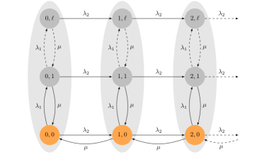
Figure 1: Transition diagram of the priority queue model.

Since there is no maximum for the number of customers in queue 1 the sub-matrices $D$, $W$ and $U$ have infinite dimension ($\ell=\infty$) and the representation below, where $d=(\lambda_{1}+\lambda_{2}+\mu)$. Note that $W_{0}$ is obtained from $W$ by replacing $d$ in its $(0,0)$ position by $(\lambda_{1}+\lambda_{2})$, since in state $(0,0)$ there are no customers in service.

$$D=\left[\begin{array}[]{ccc}\mu&0&\cdots\\ 0&0&\cdots\\ \vdots&\vdots&\ddots\end{array}\right],U=U^{0}\!\!=\!\!\left[\begin{array}[]{cccc}\lambda_{2}&0&0&\cdots\\ 0&\lambda_{2}&0&\ddots\\ 0&0&\lambda_{2}&\ddots\\ \vdots&\ddots&\ddots&\ddots\end{array}\right],W=\left[\begin{array}[]{cccc}-d&\lambda_{1}&0&\cdots\\ \mu&-d&\lambda_{1}&\ddots\\ 0&\mu&-d&\ddots\\ \vdots&\ddots&\ddots&\ddots\end{array}\right],$$

Note that in this model we have: $U^{0}=U=\lambda_{2}I,$ thus, $R^{P}=R_{1}^{P}:=-\lambda_{2}B^{-1},$ where

$$B^{P}=\left[\begin{array}[]{ccccc}-(\lambda_{1}+\mu)&\lambda_{1}&0&0&\cdots\\ \lambda_{2}+\mu&-d&\lambda_{1}&0&\cdots\\ \lambda_{2}&\mu&-d&\lambda_{1}&\ddots\\ \lambda_{2}&0&\mu&-d&\ddots\\ \vdots&\vdots&\ddots&\ddots&\ddots\end{array}\right].$$

It is clear that matrix $B^{P}$ has the required structure to use the $\text{QDESA}^{++}$. Thus, the priority queue model can be solved easily using this method.

3.2 Longest Queue

In a longest queue model, cf. [35], two types of customers arrive according to independent Poisson streams, each with rate $\lambda$ and form two queues according to their type. There is a single exponential server with rate $\mu>2\lambda$ that severs customers from the longest queue (i.e., the one having the most customers), where ties are resolved with equal probabilities for each queue; server queue switches are instantaneous.

To obtain meaningful results for this model, we will use the following state space description that is easy to work with. At each point of time let the state be specified by a tuple $(n,j)$, where $j$ denotes the difference between the two queue lengths and $n$ denotes the length of the shortest queue. A more natural state space description is discussed in Section 6.2.

It is easy to deduce that this is a DES process, in fact a homogenous level QBD process, with $M=\infty$ with level sets $\mathcal{L}_{n}$ as described in Section 2 and entrance states $(n,1)$ for level $n$ where matrices $D$, $U$, $W$ as given below, $d=2\lambda+\mu.$ We note that $W_{0}$ is obtained from $W$ by replacing $d$ in its $(0,0)$ position by $(\lambda_{1}+\lambda_{2})$, since in state $(0,0)$ there are no customers in service.

$$D=\left[\begin{array}[]{cccc}0&\mu&0&\cdots\\ 0&0&0&\cdots\\ 0&0&0&\cdots\\ \vdots&\vdots&\vdots&\ddots\end{array}\right],U=\left[\begin{array}[]{cccc}0&0&0&\cdots\\ \lambda&0&0&\ddots\\ 0&\lambda&0&\ddots\\ \vdots&\ddots&\ddots&\ddots\end{array}\right],W=\left[\begin{array}[]{cccc}-d&2\lambda&0&\cdots\\ \mu&-d&\lambda&\ddots\\ 0&\mu&-d&\ddots\\ \vdots&\ddots&\ddots&\ddots\end{array}\right].$$

Since $U^{0}=U$, the rate matrices $R_{1}$ and $R$ for this model are equal, i.e., $R_{1}^{L}=R^{L}$, as in the previous models and the matrix $B$ in this model has the following form:

$$B^{L}=\left[\begin{array}[]{ccccc}-d&2\lambda&0&0&\cdots\\ \mu&-(\mu+\lambda)&\lambda&0&\cdots\\ 0&\mu+\lambda&-d&\lambda&\ddots\\ 0&\lambda&\mu&-d&\ddots\\ 0&\lambda&0&\mu&\ddots\\ \vdots&\vdots&\ddots&\ddots&\ddots\end{array}\right].$$

Note that the matrix $B^{L}$ has a structure similar (but not identical) to that of $B$ defined in Eq. (9); its structure from the second column on is identical to that of $B$, but an extra column has been added in front. This can be easily resolved with a suitable modification of $\text{QDESA}^{++}$.

Remark 3.1.

The Feedback queue, the third model that is discussed in [21], fits the QDESA framework as well; its analysis goes analogous to the analysis of the priority queue.

4 Lattice Path Counting

A different approach to compute the steady state distribution $\pi$ for a class of Markov process that includes the queueing models described before, is the Lattice Path Counting Algorithm (LPCA) of [22], see also [21]. In this section we will repeat LPCA in the notation used in this paper.

Throughout this paper we use a labeling of states that is consistent with our notation introduced in [14] and [19]. In [21] a similar tuple notation was used, but the meaning of the first and the second element is reversed. For example, in the priority queue model of Section 3.1 we denote a system with two queues with $n$ customers in queue 2 and $i$ in queue 1 as $(n,i)$. This same $(n,i)$ in [21] denoted a system with two queues with $n$ customers in queue 1 and $i$ customers in queue 2.

Recall that we used the level (first coordinate) sets $\mathcal{L}_{n}=\{(n,i),\ i=1,\ldots,\ell\}$ where $n=0,1,\ldots$ to define a partition with respect to which the studied processes are ‘level QBD’ processes. A ‘stage QBD’ process can be defined analogously; one can rearrange the states of $\mathcal{X}$ in the order of stages (second coordinate), i.e., as $(0,1),\ldots,(M,1),$ $(0,2),\ldots(M,2),$ $\ldots,$ $(0,\ell),\ldots,$ $(M,\ell).$ In this case we define the stage sets to be: $\mathcal{K}_{i}=\{(n,i),\ n=0,1,\ldots\}.$ Transitions are allowed one stage up and one stage down to preserve the QBD property in the direction of stages. Using a stage partition, we obtain the following representation of the transition generator matrix, which will be denoted by $\widehat{Q}$ to indicate that a stage partition is used:

$$\widehat{Q}=\left[\begin{array}[]{cccc}B_{1}&B_{0}&0&\cdots\\ A_{2}&A_{1}&A_{0}&\ddots\\ 0&A_{2}&A_{1}&\ddots\\ \vdots&\ddots&\ddots&\ddots\end{array}\right],$$

where the dimension of the above sub matrices is $M\times M$.

The matrix $\widehat{Q}$ in the current paper is the same as the matrix $Q$ of [21], subject to appropriate relabeling of states, as is mentioned above. Note that in this paper the notation $M$ is used for our $\ell$ above and their corresponding $\ell$ is infinite.

Following the approach introduced in [21], a process $X(t)$ is called Lattice Path Countable (LPC) if the following three conditions hold:

• When $j>1$, the only transitions allowed from state $(n,j)$ are to states: $(n+e_{1},j+e_{2})\in\mathcal{X}$ where $e_{1}\in\{0,1\}$ and $e_{2}\in\{-1,0,1\}$;

• When $j>1$, the transition rate $\widehat{Q}((n,j)\,,\,(n+e_{1},j+e_{2}))$ is a function of the jump size and direction only, i.e.,

  $$\widehat{Q}((n,j)\,,\,(n+e_{1},j+e_{2}))=\hat{q}(e_{1},e_{2});$$ (10)

• The process is a stage QBD process where $\ell$ is infinite and $M$ is finite or infinite.

In the previous section we described a rate matrix $R$ that provides a relationship between the steady state distributions of the different levels. A similar recursion can be defined for the steady state vectors $\pi_{i}$ for stage $i>0$: $\pi_{i+1}=\pi_{i}\widehat{R},$

where $\widehat{R}$ is the minimal nonnegative solution to the matrix quadratic equation: $A_{0}+\widehat{R}A_{1}+\widehat{R}^{2}A_{2}=0.$

We have denoted the rate matrix constructed with LPC as $\widehat{R}$ to distinguish it from the matrix $R$ used in Eq. (5) above.

Figure 2 displays a simplification of a transition diagram of a process that is a QBD process with respect both to the levels and to the stages. The LPCA can be applied with respect to the stages.

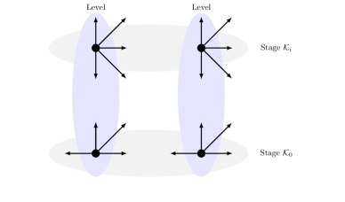
Figure 2: Levels and Stages.

Further, it is known, cf. for example [20], that the elements $\hat{r}(n|m)$ of the matrix $\widehat{R}=[\hat{r}(n|m)]$ represent the expected taboo sojourn time in $(n,i+1)$ before the first return to stage $i$ given that the process starts in $(m,i)$ multiplied by the sojourn time in stage $i$, for any $i\geq 1$. Since the LPC assumption above does not allow transitions in the downward direction and has a homogenous structure by point ii) above, the rate matrix is upper-triangular and has the following form:

$$\widehat{R}=\left[\begin{array}[]{cccc}\hat{r}_{0}&\hat{r}_{1}&\hat{r}_{2}&\cdots\\ 0&\hat{r}_{0}&\hat{r}_{1}&\cdots\\ 0&0&\hat{r}_{0}&\cdots\\ \vdots&\vdots&\ddots&\ddots\end{array}\right].$$

Theorem 4.1 below provides an explicit expression for the elements of $\widehat{R}$. It is the main result of [21] and uses the following expressions:

$$P_{h}(s,u,m) =\phi\langle 1,-1\rangle^{s}\phi\langle 1,0\rangle^{t}\phi\langle 1,1\rangle^{u}\phi\langle 0,1\rangle^{m-u}\phi\langle 0,-1\rangle^{m+1-s}$$

$$L_{h}(s,u,m) =\frac{1}{m+1}\binom{2m}{m}\binom{m+1}{s}\binom{m}{u}\binom{2m+t}{t}$$

$$G_{h} =\sum_{s=0}^{h}\sum_{u=0}^{h-s}\sum_{m=\max(u,s-1)}^{\infty}L_{h}(s,u,m)P_{h}(s,u,m)$$ (11)

$$\kappa_{h} =\frac{\phi\langle 1,0\rangle\kappa_{h-1}+\phi\langle 0,1\rangle\sum_{j=0}^{h-1}G_{h-j}\kappa_{j}+\phi\langle 1,1\rangle\sum_{j=0}^{h-1}G_{h-j-1}\kappa_{j}}{1-\phi\langle 0,1\rangle G_{0}},$$

where $\rho_{0}=1$ and $\rho_{-1}=0$ and $\phi(e_{1},e_{2})$ denotes the transition probability from state $(n,j)$ to state $(n+e_{1},j+e_{2}).$

Theorem 4.1.

The upper diagonal elements $\hat{r}_{h}$ of $\widehat{R}$ can be expressed as follows:

$$\hat{r}_{h}=2\,\frac{\phi\langle 0,1\rangle\kappa_{h}+\phi\langle 1,1\rangle\kappa_{h-1}}{1+\sqrt{1-4\phi\langle 0,1\rangle\phi\langle 0,-1\rangle}}.$$ (12)

The LPCA is based on the calculation of Eq. (12), utilizing a new computation of the $G_{h}$ in Eq. (11) above using hypergeometric functions, cf. Eq. (26) and (27) of [21].

5 Comparative Analysis

In this section we will compare the efficiency of LPCA and QDESA described in the previous section. To make a fair comparison between these algorithms we will compare their complexities in Section 5.1 for transition rate matrices on which they can both be applied. In Section 6 we discuss classes of models for which a version of QDESA is applicable while LPCA is not. We will also distinguish structures for which the LPCA can be used efficiently, but for which QDESA is not readily applicable.

It is important to note that LPCA is based on the existence of a ‘homogeneous portion’ of stages, i.e., transition rates are both stage and level independent, as is described in Section 5 of [21] and summarized in the previous section. The non-homogeneous part of the state space is considered to be (part of) stage $\mathcal{K}_{0}$. This non-homogeneous part may induce that QDESA might not be applicable; the entrance state property might be violated. Exit states might still be present, for the formal definition of an exit state we refer to [8]. In this paper we have described how an entrance state and an exit state are related and how the choice of levels can be adjusted to transform an exit state into an entrance state. However, no applications are known for which such a complex structure in $\mathcal{K}_{0}$ is necessary, that QDESA is no longer applicable.

When a process has such a structure that QDESA applies (with respect to the levels) and LPCA (with respect to the stages) we note that $B,$ (where $R=UB^{-1}$) has to have the structure of Eq. (9), up to a permutation of the columns, due to the fact that the process is a QBD process in the stage direction, see Remark 2.2. Furthermore, it is easy to see that this homogeneous structured process implies that matrix $B$ has an element homogenous structure, since the elements are independent on the stages. Summarizing the above, we state the following.

Proposition 5.1.

Suppose that the following are both true:

• LPCA is applicable to a QBD process with respect to the stages,

• The set $\bigcup_{k=0}^{n}\mathcal{L}_{k}$ has an entrance state or the set $\bigcup_{k=n}^{M}\mathcal{L}_{k}$ has an exit state.

Then $\text{QDESA}^{++}$ can be applied with respect to the level partition.

A result of this proposition is that for a fair computational comparison between the algorithms it suffices to compare LPCA with $\text{QDESA}^{++}$.

5.1 Computational Complexity of the Procedures

By Eq. (5) we know that the computational complexity of $\text{QDESA}^{++}$ is determined by the complexity of calculating the elements of the matrix $R$ with dimension $\ell\times\ell$. Since $U$ is a sparse matrix in this case, the computationally heavy step is to invert matrix $B$. For LPCA the computational complexity is determined by the complexity of calculating the elements of matrix $\widehat{R}$. Recall that $\widehat{R}$ has dimension $M\times M$.

The general result on complexity is summarized in Theorem 5.2 below. To compare the complexities of QDESA to that of LPCA, we take $\ell=M$, e.g. this is the case in the priority queue model when the queues have the same (finite or truncated) capacity. In the following complexity analysis we assume that arithmetic operations with individual elements have complexity $\mathcal{O}(1).$

Theorem 5.2.

When the steady state distribution of a QBD process can be found both by using LPCA and using QDESA the following are true:

i) Using LPCA, the computation of the stage-rate matrix $\widehat{R}$ has complexity $\mathcal{O}(M^{4}).$

ii) Using $\text{QDESA}^{++}$, the computation of the level-rate matrix $R$ has complexity $\mathcal{O}(\ell^{2}).$

Proof 5.3.

To prove part i) we assign complexity of $\mathcal{O}(h)$ to the computation of the term $\sum_{m=\max(u,s-1)}^{\infty}L_{h}(s,u,m)P_{h}(s,u,m)$ that involves hypergeometric functions, cf. Eq. (26) and Eq. (27) of [21], noting that $s+u+t=h$. The correct complexity of the above computation is actually higher, but this lower bound is easy to establish when counting conservatively. From Eq. (11) we see that to calculate $G_{h}$ we need approximately $(h^{2}/2)\mathcal{O}(h)=\mathcal{O}(h^{3})$ iterations (a double summation). The computation of matrix $\widehat{R}$ (of size $M\times M$) requires the computation of all its $M$ different nonzero elements, $\hat{r}_{0},\ldots,\hat{r}_{M-1}$ and each of these computations is of complexity $\mathcal{O}(h^{3})$. The complexity of the computation of rate matrix $\widehat{R}$ is: $\sum_{h=0}^{M-1}\mathcal{O}(h^{3})=\mathcal{O}(M^{4})$.

For part ii), we will establish the complexity for the $\text{QDESA}^{++}$. The procedure for the computations of the elements of the first row and first column of $C$ uses a single computation per element, of $\mathcal{O}(1)$. For the remaining elements a linear expression has to be solved, having a complexity of $\mathcal{O}(1)$ per element as well. Thus the total complexity of computing $C$ is $\mathcal{O}(\ell^{2})$, the number of elements of $B^{-1}$. The matrices $U$ have a sparse form (at most 3 non-zero elements per row), induced by the fact that LPCA is applicable by assumption. Since $R=UB^{-1},$ the complexity of computing $R$ is $\mathcal{O}(\ell^{2})$: both the complexity of the matrix multiplication $UB^{-1}$ and of the calculation of $B^{-1}$ have this complexity. The proof is complete.

Remark 5.4.

For some special cases, e.g. the priority queue, the complexity of LPCA is lower because of the absence of transitions from $(n,j)$ to $(n+e_{1},j+e_{2})$ with $(e_{1},e_{2})\in\{\langle-1,1\rangle,\langle 1,1\rangle\}$ for all $(n,j)$. In this special case the complexity of LPCA is $\mathcal{O}(M^{2}),$ because in the computation of $G_{h}$, both $s=0$ and $u=0$ and the summation in Eq. (11) is only over $m;$ i.e., the complexities of LPCA and QDESA are the same in this case.

Remark 5.5.

When there is no additional structure on matrix $B,$ both $\text{QDESA}^{+}$ and $\text{QDESA}^{++}$ can not be used, so we need a general matrix inversion to compute $B^{-1}$ of dimension $\ell$ by $\ell$ that is in complexity less than $\mathcal{O}(\ell^{2.379})$, cf. [32], when $\ell$ is finite. When $U$ is a non-sparse matrix this provides a solution procedure with total complexity $\mathcal{O}(l^{3})$ for QDESA.

6 The Applicability of QDESA to More General Models

In this section we will determine the differences in applicability between QDESA and LPCA, and display these differences with examples. We will consider variations of the queues in Section 3.1 and 3.2 that can be solved with QDESA but not with LPCA.

One of the main advantages of QDESA over LPCA is that QDESA not only provides a method to find the rate matrix, but the algorithm includes a way to find the steady state distribution using this rate matrix. Since LPCA does not require any restrictions on the non-homogenous part $\mathcal{K}_{0},$ the structure on this set can be very complex and a direct technique to do this step is absent and not trivial to include. Therefore QDESA can be viewed as a more complete solution procedure. And for that reason we will not discuss models that have a complicated structure on $\mathcal{K}_{0}$; even though it is possible to find the rate matrix for such a model with LPCA, but perhaps not with QDESA, within the LPCA no procedure is provided to find the steady state distribution.

There are four important classes of models for which (an extension of) QDESA is applicable and for which the LPCA can not be used at all. The first class involves element non-homogenous DES processes: in this case there is no homogeneous tail on which the LPCA is applicable. The second class involves processes with a finite number of stages $\ell$, as described in Section 2; in the LPC case there is analysis only for the case in which the number of stages $\ell$ is infinite. The third class involves DES processes with ‘down’ transitions to the entrance state in a level $L_{m-1}$ from more than one state in level $L_{m}$ for some $m$. The fourth and most general class involve all DES processes, i.e., Markov chains with transitions from an arbitrary state $(n,j)$ to states: $(n+e_{1},j+e_{2})\in\mathcal{X}$ where $e_{1}\in\{0,1,\ldots\}$ and $e_{2}\in\{\ldots,-1,0,1,\ldots\}$, under the condition of a single entrance state in the ‘down’ direction cf. [19].

Conversely, there are processes for which the LPCA is applicable, but QDESA is not. Such processes will contain transitions that destroy the DES property with respect to the level partition. For example transitions from a state $(n,1)$ to $(n-2,1)$ are allowed in an LPC Process, but are not allowed in a DES process, when $(n,1)$ is the entrance state for every level $\mathcal{L}_{n}$. However, by relabeling and changing the levels one can construct a DES process in a lot of cases.

Table 1 identifies the difference in applicability between the two procedures. We note that the transitions within the heterogenous stage $\mathcal{K}_{0}$ are not restricted, i.e. matrix $B_{0}$ and $B_{1}$ are possibly non-sparse matrices in the LPCA procedure. We compare this with the restrictions that are imposed by QDESA.

Stage $\mathcal{K}_{0}$, the Non-Homogeneous portion
LPCA	QDESA
Within this stage all transitions allowed.	QSF Structure should be obeyed.
Transitions leaving $\mathcal{K}_{0}$ allowed only to $\mathcal{K}_{1}$.	Transitions are allowed to all higher stages.
Element Non-Homogeneous.	Element Non-Homogeneous.
Sol. Proc. on $\mathcal{K}_{0}$ not included in algorithm.	Solution procedure included for all levels.
Stage $\mathcal{K}_{i}$ from the Homogeneous portion
LPCA	QDESA
Nearest Neighbor structure within levels.	All transitions allowed within levels.
Nearest Neighbor to ‘NE’, ‘E’, ‘SE’.	All transitions allowed to higher levels.
Element Homogeneous.	Element Non-Homogeneous.
No transitions to ‘NW’, ‘W’, ‘SW’ allowed.	Trans. to ‘W’ allowed to entrance state.
Number of stages must be infinite.	Number of stages can be finite or infinite.

Table 1: Restrictions for the applicability of LPCA and QDESA.

6.1 The Priority Queue with Batch Arrivals

Consider the priority queue model where two types of customers arrive in batches according to independent Poisson processes with rate $\lambda_{i}$ for queue $i$, $i=1,2$. Upon arrival the size $Z_{i}$ of a batch of type $i$ becomes known. For each fixed $i$ the $Z_{i}$ are iid random variables that follow a known discrete distribution: $P(Z_{i}=z)=p_{i}(z).$

There is a single server that serves at exponential rate $\mu,$ independent of the arrival processes. The server serves customers at queue 2 only when queue 1 is empty, preemptions are allowed and switches are instantaneous. Under these assumptions the state of the system can be summarized by a tuple $(n,j)$ where $n$ (respectively $j$) is the number of customers in queue 2 (respectively in queue 1). Because we assume that there is no maximum for number of customers in queue 1 the sub-matrices of $Q$ have infinite dimension. It is easy to see that $Q$ is the transition rate matrix of a successively lumpable process with respect to the levels with $M_{1}=0,$ $M_{2}=\infty$ and the following within- and up-matrices, where $d=(\lambda_{1}+\lambda_{2}+\mu)$:

$$W=\left[\begin{array}[]{cccc}-d&\lambda_{1}p_{1}(1)&\lambda_{1}p_{1}(2)&\cdots\\ \mu&-d&\lambda_{1}p_{1}(1)&\ddots\\ 0&\mu&-d&\ddots\\ \vdots&\ddots&\ddots&\ddots\end{array}\right],\quad U^{nk}=\left[\begin{array}[]{cccc}\lambda_{2}p_{2}(k)&0&0&\cdots\\ 0&\lambda_{2}p_{2}(k)&0&\ddots\\ 0&0&\lambda_{2}p_{2}(k)&\ddots\\ \vdots&\ddots&\ddots&\ddots\end{array}\right].$$

The matrix $W^{0}$ has its $(1,1)$ element equal to $-(\lambda_{1}+\lambda_{2})$ and all its other elements are the same as those of $W$. The matrix $D$ is the same as that of the process described in Section 3.1. This model can be solved using QDESA, but LPCA is not applicable.

6.2 Longest Queue Model with non-homogeneous arrival rates

We will extend the model discussed in Section 3.2 in such a way that now two types of customers arrive according to independent Poisson streams, with rate $\lambda_{1}$ and $\lambda_{2}$. There is a single exponential server with rate $\mu>\lambda_{1}+\lambda_{2}$. Note that the fact that the arrivals have a different rate implies that the state space description used in Section 3.2 does not induce a Markov chain. Therefore, we now let the state be specified by a tuple $(n,j)$ where $j$ denotes the number of customers in queue 1 and $n$ the number of customers in queue 2. The buffers are of size $M$ and $\ell$ respectively and can be either finite of infinite. The transition diagram is displayed in Figure 3 and the level partition is highlighted by the grey background. It is easy to deduct that this is a DES process where the level sets $\mathcal{L}$ are formally described as follows:

$$\mathcal{L}_{m}=\bigcup_{n=m}^{M}\{(n,m-1)\}\cup\bigcup_{i=m}^{\ell}\{(m-1,\ell)\}\cup\{(m,m)\}.$$

State $(m,m)$ is the entrance states for the set $\bigcup^{m}_{k=0}\mathcal{L}_{k}.$ With this different arrival rates, LPCA can not be used, while $\text{QDESA}^{+}$ can be used. Note that the rate matrix $R_{m}$ depends on the level $m$.

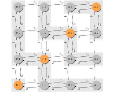
Figure 3: Longest Queue model.

This Research has been partially supported by the National Science Foundation with grant CMMI-14-50743.

References

- [1] Adan, I., Economou, A. and Kapodistria, S. (2009). Synchronized reneging in queueing systems with vacations. Queueing Systems 62, 1–33.
- [2] Adan, I. J., Boxma, O. J., Kapodistria, S. and Kulkarni, V. G. (2015). The shorter queue polling model. Annals of Operations Research to appear.
- [3] Adan, I. J., Kapodistria, S. and van Leeuwaarden, J. S. (2013). Erlang arrivals joining the shorter queue. Queueing Systems 74, 273–302.
- [4] Bini, D., Meini, B., Steffé, S. and Van Houdt, B. (2006). Structured markov chains solver: software tools. In Proceeding from the 2006 workshop on Tools for solving structured Markov chains. ACM. Pisa, Italy. p. 14.
- [5] Böhm, W., Krinik, A. and Mohanty, S. (1997). The combinatorics of birth-death processes and applications to queues. Queueing Systems 26, 255–267.
- [6] Bright, L. and Taylor, P. (1995). Calculating the equilibrium distribution in level dependent quasi-birth-and-death processes. Stochastic Models 11, 497–525.
- [7] Eisenblätter, A., Wessäly, R., Martin, A., Fügenschuh, A., Wegel, O., Koch, T., Achterberg, T. and Koster, A. (2003). Modelling feasible network configurations for UMTS. In Telecommunications Network Design and Management. Springer, United States.
- [8] Ertiningsih, D., Katehakis, M., Smit, L. and Spieksma, F. (2015). QSF processes with level product form stationary distributions. Under review at Naval Research Logistics.
- [9] Etessami, K., Wojtczak, D. and Yannakakis, M. (2010). Quasi-birth–death processes, tree-like QBDs, probabilistic 1-counter automata, and pushdown systems. Performance Evaluation 67, 837–857.
- [10] Flajolet, P. and Guillemin, F. (2000). The formal theory of birth-and-death processes, lattice path combinatorics and continued fractions. Advances in Applied Probability 32, 750–778.
- [11] Gillent, F. and Latouche, G. (1983). Semi-explicit solutions for M/PH/1-like queuing systems. European journal of operational research 13, 151–160.
- [12] Hager, W. (1989). Updating the inverse of a matrix. SIAM review 31, 221–239.
- [13] Heinig, G. and Rost, K. (1984). Algebraic methods for Toeplitz-like matrices and operators. Springer, Basel, Switserland.
- [14] Katehakis, M. and Smit, L. (2012). A successive lumping procedure for a class of Markov chains. Probability in the Engineering and Informational Sciences 26, 483–508.
- [15] Katehakis, M., Smit, L. and Spieksma, F. (2014). A solution to a countable system of equations arising in stochastic processes. Under review.
- [16] Katehakis, M. N. and Derman, C. (1989). On the maintenance of systems composed of highly reliable components. Management Science 35, 551–560.
- [17] Katehakis, M. N. and Melolidakis, C. (1988). Dynamic repair allocation for a K out of N system maintained by distinguishable repairmen. Probability in the Engineering and Informational Sciences 2, 51–62.
- [18] Katehakis, M. N. and Smit, L. C. (2012). On computing optimal (q, r) replenishment policies under quantity discounts. Annals of Operations Research 200, 279–298.
- [19] Katehakis, M. N., Smit, L. C. and Spieksma, F. M. (2015). DES and RES processes and their explicit solutions. Probability in the Engineering and Informational Sciences FirstView, 1–27.
- [20] Latouche, G. and Ramaswami, V. (1999). Introduction to matrix analytic methods in stochastic modeling vol. 5. SIAM, Philadelphia, PA.
- [21] Leeuwaarden, J. van, Squillante, M. and Winands, E. (2009). Quasi-birth-and-death processes, lattice path counting, and hypergeometric functions. Journal of Applied Probability 46, 507–520.
- [22] Leeuwaarden, J. van and Winands, E. (2006). Quasi-birth-and-death processes with an explicit rate matrix. Stochastic models 22, 77–98.
- [23] Liu, D. and Zhao, Y. (1996). Determination of explicit solutions for a general class of Markov processes. Matrix-Analytic Methods in Stochastic Models 343–358.
- [24] Mohanty, S. (1979). Lattice path counting and applications. Academic Press, New York, NY.
- [25] Mohanty, S. and Panny, W. (1990). A discrete-time analogue of the M/M/1 queue and the transient solution: A geometric approach. Sankhyā: The Indian Journal of Statistics, Series A 364–370.
- [26] Neuts, M. (1981). Matrix-geometric solutions in stochastic models. The Johns Hopkins University Press, Baltimore, MD.
- [27] Perros, H. (1994). Queueing Networks with Blocking. Oxford University Press, New York, NY.
- [28] Spitzer, F. (2001). Principles of random walk vol. 34. Springer Verlag, New York, NY.
- [29] Ulukus, M. Y., Güllü, R. and Örmeci, L. (2011). Admission and termination control of a two class loss system. Stochastic Models 27, 2–25.
- [30] Van Houdt, B. and Leeuwaarden, J. van (2011). Triangular M/G/1-type and tree-like quasi-birth-death Markov chains. INFORMS Journal on Computing 23, 165–171.
- [31] Vlasiou, M., Zhang, J. and Zwart, B. (2014). Insensitivity of proportional fairness in critically loaded bandwidth sharing networks. arXiv preprint arXiv:1411.4841.
- [32] Williams, V. (2012). Multiplying matrices faster than Coppersmith-Winograd. In Proceedings of the 44th symposium on Theory of Computing. ACM. New York, NY. pp. 887–898.
- [33] Woodbury, M. (1950). Inverting modified matrices. Memorandum report 42, 106.
- [34] Zhao, Y. and Grassmann, W. (1995). Queueing analysis of a jockeying model. Operations research 43, 520–529.
- [35] Zheng, Y.-S. and Zipkin, P. (1990). A queueing model to analyze the value of centralized inventory information. Operations Research 38, 296–307.