The Quasar-LBG two-point angular cross-correlation function at $z\sim$ 4
in the COSMOS field

Abstract

In order to investigate the origin of quasars, we estimate the bias factor for low-luminosity quasars at high redshift for the first time. In this study, we use the two-point angular cross-correlation function (CCF) for both low-luminosity quasars at $-24<M_{\rm 1450}<-22$ and Lyman-break galaxies (LBGs). Our sample consists of both 25 low-luminosity quasars (16 objects are spectroscopically confirmed low-luminosity quasars) in the redshift range $3.1<z<4.5$ and 835 color-selected LBGs with $z^{\prime}_{\rm LBG}<25.0$ at $z\sim 4$ in the COSMOS field. We have made our analysis for the following two quasar samples; (1) the spectroscopic sample (the 16 quasars confirmed by spectroscopy), and (2) the total sample (the 25 quasars including 9 quasars with photometric redshifts). The bias factor for low-luminosity quasars at $z\sim 4$ is derived by utilizing the quasar-LBG CCF and the LBG auto-correlation function. We then obtain the $86\%$ upper limits of the bias factors for low-luminosity quasars, that are 5.63 and 10.50 for the total and the spectroscopic samples, respectively. These bias factors correspond to the typical dark matter halo masses, log $(M_{\rm DM}/(h^{-1}M_{\odot}))=$$12.7$ and $13.5$, respectively. This result is not inconsistent with the predicted bias for quasars which is estimated by the major merger models.

1. Introduction

The observed close relationship between the mass of the spheroidal component of a galaxy and its central supermassive black hole (SMBH) suggests that the evolution of galaxies and SMBHs are closely related (e.g., Marconi & Hunt 2003; Häring & Rix 2004; McConnell & Ma 2013). Accordingly some important questions arise as when and how such a co-evolution has been established and what physical processes are essentially important. A straightforward approach to explore these issues is investigating the statistical properties of quasars at high redshifts, where the quasar activity (that corresponds to the growth of SMBHs) is much more active than in the local universe (e.g., Richards et al. 2006; Croom et al. 2009a), because different evolutionary scenarios for SMBHs predict different statistical properties of quasars as function of redshift (e.g., Hopkins et al. 2007).

The quasar activity is thought to be powered by mass accretion onto a SMBH at the center of massive galaxies (Rees 1984). The most efficient gas fueling mechanism is thought to be major and minor mergers of galaxies (e.g., Sanders et al. 1988; Taniguchi 1999; see also Taniguchi 2013). Therefore, in order to constrain the triggering mechanism for quasar activity, we need detailed studies of environmental properties of quasars.

Motivated by these considerations, the two-point auto-correlation function (ACF) of quasars has been studied based on wide-field survey data, e.g., 2dF Quasar Redshift Survey and Sloan Digital Sky Survey (e.g., Croom et al. 2005; Porciani & Norberg 2006; Myers et al. 2006, 2007; Shen et al. 2007; da Ângela et al. 2008; Shen et al. 2009; Ross et al. 2009; Ivashchenko et al. 2010; White et al. 2012). The ACFs have also been investigated for active galactic nuclei (AGNs) including quasars selected through X-ray data (e.g., Miyaji et al. 2007; Ueda et al. 2008; Gilli et al. 2009; Starikova et al. 2011; Krumpe et al. 2012; Koutoulidis et al. 2013; Allevato et al. 2014). Most of these studies have shown that luminous AGNs tend to live in massive dark matter halos ($\sim 10^{12}-10^{13.5}h^{-1}M_{\odot}$), suggesting that luminous AGN activity is triggered by galaxy mergers because such massive dark matter halos could be assembled by successive mergers of small dark matter halos. It is also reported that galaxy mergers do not account for the majority of the moderate X-ray luminous AGNs at $z\lesssim 2.2$ (Allevato et al. 2011). However, it is difficult to investigate small-scale clustering properties of quasars because of their low number density.

Here it should be noted that the mass of dark-matter halos hosting quasars can be estimated also through the two-point cross-correlation function (CCF) for quasars and galaxies, combined with the ACF for galaxies. The advantage of the CCF is that the required size of the quasar sample is relatively smaller than the ACF analysis, though we need enough number of galaxies around quasars for the CCF analysis. In addition, it is possible to study the small-scale clustering properties of quasars through the CCF, that is too challenging for the ACF study. Therefore, in order to understand the triggering mechanism of quasar activity, it is useful to investigate the CCF for quasars and galaxies around them. Several pioneering studies have been made to date (e.g., Adelberger & Steidel 2005; Padmanabhan et al. 2009; Mountrichas et al. 2009; Coil et al. 2009; Miyaji et al. 2011; Hickox et al. 2011; Zhang et al. 2013; Shirasaki et al. 2011; Mountrichas & Georgakakis 2012; Komiya et al. 2013; Shen et al. 2013; Krolewski & Eisenstein 2015). For instance, Zhang et al. (2013) investigated the spatial clustering of galaxies around quasars at redshifts from 0.6 to 1.2. They found that the clustering amplitude is significantly larger for quasars with more massive black holes, or with bluer colors, while there is no dependence on quasar luminosity. This suggests that the mass of dark matter halos in which quasars reside is not correlated with the quasar luminosity. In addition, it is possible that the triggering mechanism of high- and low-luminosity quasars may be the same in this luminosity range.

The CCF of quasars and galaxies has also been investigated at higher redshifts. Shirasaki et al. (2011) investigated the projected CCF of AGNs and galaxies at redshifts from 0.3 to 3.0 and found significant excess of galaxies around the AGNs. They found that AGNs at higher redshifts reside in denser environments than those at lower redshifts. This suggests that major mergers are the preferred mechanism to trigger AGN activity at high redshifts. They also reported that there is no luminosity dependence of AGN clustering. At $z\sim 3$, Francke et al. (2008) studied the two-point angular CCF of AGNs and Lyman break galaxies (LBGs) (see also Bielby et al. 2011) and found that AGNs tend to be clustered more strongly than LBGs. They also found no luminosity dependence of AGN clustering. At $z>3$, clustering of LBGs around quasars has been recently studied (e.g., Husband et al. 2013). However the luminosity dependence of quasar clustering is not studied, due to the lack of adequate samples of low-luminosity quasars and galaxies around them. Therefore, the triggering mechanism of low-luminosity quasars at $z>3$ has not yet been studied so far.

Motivated by the situation described above, we study the two-point angular CCF of the 25 low-luminosity quasars (16 objects are spectroscopically confirmed low-luminosity quasars) and 835 LBGs in the redshift range $3.1<z<4.5$ in the COSMOS field. Then we derive the bias factor for low-luminosity quasars and constrain the dark matter halo mass in which low-luminosity quasars at $z\sim 4$ exist. The outline of this paper is as follows. In Section 2, we describe the data of low-luminosity quasars focused in this study and the method used for the photometric selection of LBG candidates. In Section 3, we report the results of the clustering analysis of quasars and LBGs. In Section 4 and 5, we give our discussion and summary. Throughout this paper we adopt a $\Lambda$CDM cosmology with $\Omega_{m}$ = 0.3,  $\Omega_{\Lambda}$ = 0.7, $\sigma_{\rm 8}$ = 0.9, and a Hubble constant of $H_{0}$ = 70 km s^-1 Mpc^-1. We use the AB magnitude system. All of the errors reported in this paper are 1 sigma.

2. The Sample

2.1. The Cosmic Evolution Survey

Wide and deep multi-wavelength data are publicly available in the Cosmic Evolution Survey (COSMOS) field (Scoville et al. 2007). Therefore we can select large numbers of high-$z$ galaxies and quasars in the same field to study their statistical properties such as the CCF. Another advantage of the COSMOS dataset is the dense sampling in the optical wavelength with intermediate-band filters, that makes the estimates of the photometric redshifts of galaxies far more accurate than in other deep-survey fields (Ilbert et al. 2009; see also Cardamone et al. 2010). For the above reasons, we decided to focus on the COSMOS field for the CCF analysis at $z\sim 4$.

COSMOS is a treasury program of the Hubble Space Telescope (HST). It comprises 270 and 320 orbits allocated in the HST Cycles 12 and 13, respectively (Scoville et al. 2007; Koekemoer et al. 2007). The COSMOS field covers an area of $\sim\rm 1.4^{\circ}\times 1.4^{\circ}$ square which corresponds to $\sim 2\deg^{2}$, centered at R.A. (J2000) = 10:00:28.6 and Dec. (J2000) =+02:12:21.0. We use an upgraded version of the photometric redshift catalogue from Ilbert et al. (2009) (see also Capak et al. 2007) including the new UltraVISTA data from the DR1 release (McCracken et al. 2012), to select samples of both quasars and LBGs at $z\sim 4$. This catalog covers an area of $\sim$ 2 $\rm deg^{2}$ and contains several photometric measurements. Specifically in this paper, we use the $u^{*}$-band $3^{{}^{\prime\prime}}$ diameter aperture apparent magnitude measured on the image obtained with MegaCam (Boulade et al. 2003) on the Canada-France-Hawaii Telescope (CFHT), and the $3^{{}^{\prime\prime}}$ diameter aperture apparent magnitudes of the $g^{\prime}$-, $r^{\prime}$-, and $z^{\prime}$-bands (Taniguchi et al. 2007) measured on the image obtained with the Subaru Suprime-Cam (Miyazaki et al. 2002). The 5$\sigma$ limiting AB apparent magnitudes are $u^{*}$ = 26.5, $g^{\prime}$ = 26.5, $r^{\prime}$ = 26.6, and $z^{\prime}$ = 25.1 ($3^{{}^{\prime\prime}}$ diameter aperture). We also use the Advanced Camera for Surveys (ACS) catalog (Koekemoer et al. 2007; Leauthaud et al. 2007) when we select the low-luminosity quasars to separate galaxies from point sources (see Ikeda et al. 2011, 2012 for more details).

2.2. Selection for Quasars at $z\sim 4$

In order to calculate the bias factor for low-luminosity quasars at $z\sim 4$, we need a low-luminosity quasar sample. Ikeda et al. (2011) identified eight low-luminosity quasars through spectroscopic follow-up observations for their optical color-selected photometric quasar candidates. Additional low-luminosity quasars were also found by using the multi-wavelength imaging data including the optical broad, intermediate, narrowband, near-infrared and Spitzer/IRAC photometric measurements (Masters et al. 2012). To select low-luminosity quasars at $z\sim 4$ in the COSMOS field we used the following selection criteria:

$$-24.0<M_{\tt 1450}<-22.0,$$ (1)

and,

$$3.1<z<\rm 4.5.$$ (2)

Note that we adopt both $z$ and $M_{\tt 1450}$ given in Masters et al. (2012). Then we reject objects which lie in masked regions (Capak et al. 2007). As a result, we selected 25 quasars at $3.1<z<4.5$. Among them, 16 objects are spectroscopically confirmed quasars. We refer this sample as the spectroscopic sample while the sample of 25 quasars is as the total one. Total sample have been selected by utilizing the 29-band photometric data to remove contaminants. Since they have been selected by utilizing such a lot of photometric data, we consider that the contamination rate for total sample is to be very low. Table 1, Figure 1, and Figure 2 show properties of these quasars, their redshift distribution, and their magnitude distribution, respectively. The median, mean, and the standard deviation of the redshift of the 25 quasars (16 spectroscopically confirmed quasar redshift) are 3.45 (3.59), 3.59 (3.68), and 0.40 (0.40), respectively.

Table 1Properties of the low-luminosity quasars at $z\sim 4$

IDa		R.A.	Decl.	$M_{\tt 1450}$	$z_{\rm sp}$	$z_{\rm adopt}^{b}$
		(deg)	(deg)	(mag)
298002		150.43706	1.649305	$-22.34$	3.89	3.89
329051		150.16891	1.774590	$-22.71$	–	4.35
330806		150.10738	1.759201	$-22.85$	4.14	4.14
381470		149.85396	1.753672	$-22.11$	–	3.30
422327		149.70151	1.638375	$-22.49$	3.20	3.20
507779		150.48563	1.871927	$-23.78$	4.45	4.45
519634		150.27715	1.958373	$-22.61$	–	3.40
710344		150.62828	2.006204	$-22.06$	–	3.45
804307		150.00438	2.038898	$-23.56$	3.50	3.50
887716		149.49590	1.968019	$-22.38$	–	3.23
1046585		149.85153	2.276400	$-22.39$	3.37	3.37
1060679		149.73622	2.179933	$-22.23$	4.20	4.20
1110682		149.50595	2.185332	$-22.71$	–	3.28
1159815		150.63844	2.391350	$-22.98$	3.65	3.65
1163086		150.70377	2.370019	$-23.00$	3.75	3.75
1271385		149.86966	2.294046	$-23.42$	3.35	3.35
1273346		149.77692	2.444306	$-22.65$	4.16	4.16
1371806		150.59184	2.619375	$-22.10$	–	3.12
1465836		150.13036	2.466012	$-22.56$	3.86	3.86
1575750		150.73715	2.722578	$-22.78$	3.32	3.32
1605275		150.62006	2.671402	$-22.82$	3.14	3.14
1657280		150.24078	2.659058	$-22.74$	3.36	3.36
1719143		149.75539	2.738555	$-22.26$	3.52	3.52
1730531		149.84322	2.659095	$-22.15$	–	3.51
1743444		149.66605	2.740230	$-22.54$	–	3.15

^a ID for Table 3 of Masters et al. (2012).
^b Redshift given by Masters et al. (2012) and adopted in our analysis.

2.3. Selection for Lyman Break Galaxies at $z\sim 4$

We also select a sample of Lyman break galaxies (LBGs) in the redshift range $3.1<z<4.5$ in the COSMOS field, utilizing the two color diagram of $r^{\prime}-z^{\prime}$ vs. $g^{\prime}-r^{\prime}$ (Figure 3). For the selection of LBGs at $z\sim 4$, we adopt the following selection criteria:

$$149.411400<{\tt R.A.(degree)}<150.826934,$$ (3)

$$1.49878<{\tt Decl.(degree)}<2.91276,$$ (4)

$$z^{\prime}<25.0,$$ (5)

$$u^{*}\geq 27.05,$$ (6)

$$g^{\prime}-r^{\prime}\geq 1.0,$$ (7)

$$g^{\prime}-r^{\prime}>1.1(r^{\prime}-z^{\prime})+1.1,$$ (8)

and,

$$r^{\prime}-z^{\prime}\leq 1.5,$$ (9)

where $u^{*}$ = 27.05 corresponds to the 3$\sigma$ limiting magnitude in the $u^{*}$-band. The criterion (8) is adopted to select LBGs without significant contamination from low-$z$ elliptical galaxies (see Figure 3). In order to remove low-$z$ objects, we add the criteria (6), (7), and (9). These selection criteria are adjusted to select LBGs with photometric redshifts ($z_{\rm ph}$), whose distribution is similar to the redshift distribution of our quasar sample. We also remove eight spectroscopically confirmed quasars satisfying the above criteria from the LBG sample, because those 8 objects are not LBGs apparently. Note that seven objects among the eight removed objects are included in our quasar sample while the remaining one object is not, because its magnitude ($M_{1450}=-20.91$) is out of the magnitude range of our quasar sample ($-22<M_{\rm 1450}<-24$).

As a result, we obtain a sample of 835 LBGs at $z\sim 4$ in the COSMOS field. We use the upgraded photometric redshift (originally described in Ilbert et al. 2009 with including the new UltraVISTA DR1 data) to investigate the photometric redshift distribution of the color-selected galaxies. Figure 4 shows the photometric redshift distribution of color-selected galaxies. The median, mean, and the standard deviation of the redshift of the color-selected galaxies are 3.59, 3.13, and 1.32, respectively. As shown in Figure 4, there are some low-$z$ ($z<1$) galaxies in the color-selected LBG sample. We consider that most of these contaminants are low-$z$ elliptical galaxies, being inferred from the color track of the model elliptical galaxy shown in Figure 3. Note that it is difficult to remove these low-$z$ contaminants by modifying the adopted color-selection criteria, because the optical colors of LBGs and those contaminants are similar. The median, mean, and the standard deviation of the photometric redshift of the color-selected galaxies, after removing objects whose photometric redshifts are below 3, are 3.67, 3.71, and 0.62, respectively. These results are similar to that of low-luminosity quasars in this work. The typical error of the photometric redshift for the color-selected LBGs is $\sim 0.1$. There are 67 spectroscopically confirmed objects in our color-selected galaxies and their redshift distribution is shown in Figure 5. We confirm that the spectroscopic redshift distribution of color-selected galaxies is also similar with that of low-luminosity quasars in this paper.

Figure 1.— Redshift distribution of the low-luminosity quasars at $3.1<z<4.5$ used in this work. Upper and lower panels show the redshift distribution of 25 low-luminosity quasars (total) and 16 spectroscopically confirmed low-luminosity quasars, respectively.

Figure 6 shows the magnitude distribution of the color-selected galaxies used in this paper and we also confirm that the magnitude distribution of the spectroscopic sample does not drops at a much brighter limit than that of the full photometric sample. These results may be somewhat surprising, in the sense that any spectroscopic sample tends to be brighter than the photometric sample in the same survey generally. However in our case, we are now focusing only on relatively bright LBGs even for the photometric sample, whose magnitude is much brighter than the limiting magnitude of the COSMOS survey. This is because we would like to remove most contaminants from our sample and select our sample whose errors of photometric redshift are as small as possible. In addition, it is also expected that bright LBGs and the quasar sample show a strong correlation because it is reported that the LBG clustering becomes strong with increasing UV luminosity (e.g., Ouchi et al. 2004), and then it is considered that brighter LBGs exist in more massive dark matter halos. Therefore bright LBGs are useful to investigate the clustering of quasars and galaxies. As our measured CCF and ACF will become weaker than the real CCF and ACF due to these low-$z$ galaxies, we correct our CCF and ACF by utilizing the contamination rate for color-selected galaxies (see Sections 3.1 and 3.2).

Figure 2.— Magnitude distribution of the low-luminosity quasars at $3.1<z<4.5$ used in this work. Upper and lower panels show the magnitude distribution of 25 low-luminosity quasars (total) and 16 spectroscopically confirmed low-luminosity quasars, respectively.

3. Clustering Analysis of quasars and LBGs

3.1. Quasar-LBG Two-Point Angular Cross-Correlation Function at $z\sim 4$

Using the samples of quasars and LBGs described in Sections 2.2 and 2.3, we calculate the quasar-LBG two-point angular CCF, $\omega_{\rm QL}$ ($\theta$), at $z\sim 4$ using the following equation (Croft et al. 1999; Francke et al. 2008):

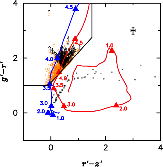
Figure 3.— Two-color diagram of $g^{\prime}-r^{\prime}$ vs. $r^{\prime}-z^{\prime}$, that we use for $z\sim 4$ LBG selection. Orange circles denote the LBG candidates with $z^{\prime}<25.0$. Orange circles with a black arrow show the LBG candidates which are not detected in $g^{\prime}$-band at 3 sigma limiting magnitude, $g^{\prime}=27.05$ (242 objects among 835 objects). For those cases, the 3$\sigma$ lower limit of their $g^{\prime}-r^{\prime}$ color is plotted. The blue and red lines are the color track of the model star-forming galaxy (where the instantaneous-burst model of Bruzual & Charlot 2003 with a metallicity of $Z=0.02$, an age of 0.025 Gyr and a Ly$\alpha$ equivalent width $=21\rm\AA$ (Jones et al. 2012) are adopted) and elliptical galaxy colors (where the stellar population model of Bruzual & Charlot 2003 with a metallicity of $Z=0.02$ and an exponential decay time of $\tau$= 1 Gyr are adopted, and the ages of the model elliptical is 8 Gyr). The IGM absorption is corrected by adopting the model of Madau (1995), for both color tracks. Triangles denote the color of the model elliptical and star-forming galaxy at $z=1.0$, 2.0, 3.0, 3.5, 4.0, and 4.5, respectively. Black asterisks show colors of G, K, and M-type stars (Pickles 1998). The black solid line shows our photometric criteria used to select LBG candidates at $z\sim 4$. The error bar of the upper right side in this Figure denotes 1$\sigma$ error for the $g^{\prime}-r^{\prime}$ and $r^{\prime}-z^{\prime}$ of our LBG candidates.

$$\rm\omega_{\rm QL}(\theta)=\it\frac{\langle D_{\rm Q}D_{\rm L}\rangle}{\it\langle D_{\rm Q}R\rangle}-\rm 1,$$ (10)

where $\langle D_{\rm Q}D_{\rm L}\rangle$ and $\langle D_{\rm Q}R\rangle$ are the normalized quasar-LBG and quasar-random number of pairs defined as follows:

$$\langle D_{\rm Q}D_{\rm L}\rangle=\frac{D_{\rm Q}D_{\rm L}(\theta)}{\it N_{\rm Q}\it N_{\rm L}},$$ (11)

and,

$$\langle D_{\rm Q}R\rangle=\frac{D_{\rm Q}R(\theta)}{\it N_{\rm Q}\it N_{\rm R}},$$ (12)

where $D_{\rm Q}D_{\rm L}(\theta)$ and $D_{\rm Q}R(\theta)$ are the number of data-data and data-random pairs at angular separation $\theta\pm\Delta\theta$, respectively. In the equations (11) and (12), $N_{\rm Q}$, $N_{\rm L}$, and $N_{\rm R}$ are the total number of the quasar, LBG, and random sample, respectively. We create the 100,000 random samples which are avoiding the masked regions and we calculate the quasar-LBG CCF. The errors in $\omega_{\rm\small QL}(\theta)$ are estimated by the bootstrap method as follows (Ling et al. 1986):

$$\sigma_{\omega_{\rm QL}}=\Bigl{\{}\sum_{i=1}^{N}\frac{[\omega_{i}(\theta)-\langle\omega(\theta)\rangle]^{2}}{N-1}\Bigl{\}}^{1/2},$$ (13)

where $N$ is the number of bootstrap samples and $\langle\omega(\theta)\rangle$ is calculated as follows:

$$\langle\omega(\theta)\rangle=\sum_{i=1}^{N}\frac{\omega_{i}(\theta)}{N}.$$ (14)

We use $N=1,000$, and Figure 5 shows the result of the quasar-LBG two-point angular CCF at $z\sim 4$. Previous investigators mentioned that the Poisson error becomes increasingly inaccurate at larger scale (e.g., Mountrichas et al. 2009). We also confirmed that the errors which are calculated by the bootstrap method are about two times larger than the Poisson errors. We calculate the CCF for both total and spectroscopic samples. We summarize $\omega_{\rm QL}(\theta)$ and errors of $\omega_{\rm QL}(\theta)$ in Table 2. The observed two-point angular CCF is approximated by a power law form at large scales as follows:

$$\omega_{\rm QL}(\theta)=A_{\omega}^{\rm CCF}(\theta^{-\beta}-\rm C),$$ (15)

where $\beta$ is fixed to be 0.8 (Francke et al. 2008) and C is the integral constraint (Groth & Peebles 1977). To avoid the one-halo term and negative value at the second bin, we do not use $\rm\omega_{\rm QL}(\theta)$ on smaller scales ($\rm angular\ separation<80$ arcsec) to calculate $A_{\omega}^{\rm CCF}$. Here we estimate the integral constraint as follows:

Figure 4.— Photometric redshift distribution of the 835 color-selected galaxies used in this paper.

Figure 5.— Spectroscopic redshift distribution of the 67 objects among the 835 color-selected galaxies used in this paper.

$$\rm C=\frac{\Sigma\it RR(\theta)\theta^{\rm-0.8}}{\Sigma\it RR(\theta)}.$$ (16)

We calculate C and a value of C = 0.00601 in this case. Using equation (15) and (16), we calculate $A_{\omega}^{\rm CCF}$ to fit the two-point angular CCF. As a result, we obtain $A_{\omega}^{\rm CCF}$ = 1.77${}^{+1.66}_{-0.86}$ and 3.33${}^{+3.06}_{-1.60}$ for the total and the spectroscopic samples, respectively.

Figure 6.— Magnitude distribution of the color-selected galaxies used in this paper. Upper and lower panels show the magnitude distribution of 835 color-selected galaxies (total) and 67 spectroscopically confirmed galaxies at $z\sim 4$, respectively.

Since we use the photometric sample of LBGs, the derived correlation amplitude is affected by some contamination of galaxies at lower redshifts. Accordingly the effect of the contamination on the derived correlation amplitude should be corrected. We estimated the contamination rate, $f_{\rm c}$, utilizing the distribution of spectroscopic redshifts in our LBG sample (see Figures 5). In a naive estimate, the contamination rate is calculated through the following formula using the spectroscopic redshift of our color-selected LBGs: $f_{\rm c}=(N(z_{\rm sp}<3.1)+N(z_{\rm sp}>4.5))/N_{\rm total}$, where the numbers of contaminating objects are $N(z_{\rm sp}<3.1)=2$ and $N(z_{\rm ph}>4.5)=0$, among our color-selected and spectroscopically confirmed objects ($N_{\rm total}=67$). Therefore the contamination rate in our color-selected LBG sample is estimated to be $f_{\rm c}=2/67\sim 0.03$. In order to calculate $A_{\omega}$ (CCF) accurately, we need to calculate the contamination rate in the total sample for low-luminosity quasars. Therefore we calculate the contamination rate for the total sample, $f_{\rm cq}$, as follows:

$$f_{\rm cq}=\int^{M=-22}_{M=-24}\frac{n_{\rm total}(M)[f_{\rm r}\Phi_{\rm LBG}(M)/\Phi_{\rm QSO}(M)]dM}{N_{\rm total}},$$ (17)

where $f_{\rm r}$, $n_{\rm total}(M)$, $\Phi_{\rm LBG}(M)$, $\Phi_{\rm QSO}(M)$, and $N_{\rm total}$ are the fraction which high-redshift galaxies pass quasar selections, the magnitude distribution of low-luminosity quasars for total sample, the luminosity function of LBGs, the luminosity function of quasars, and the total number of low-luminosity quasars, respectively. Masters et al. (2012) estimated $f_{\rm r}$ and they found that only 2 objects among 386 spectroscopically confirmed high-redshift galaxies are pass their quasar selection. Therefore $f_{\rm r}$ is estimated to be $\sim 0.005$. We use $\Phi_{\rm LBG}(M)$ which are derived by Bouwens et al. (2007) and $\Phi_{\rm QSO}(M)$ which are derived by Masters et al. (2012), in this paper. Using above results and Equation (17), we calculate $f_{\rm cq}$ and the calculated $f_{\rm cq}$ is $\sim 0.05$. Since the contamination rate for the total sample is so low, we do not worry about impact on the CCF due to include high-redshift galaxies in the total sample. Even if some high-redshift galaxies such as bright LBGs are including in the total sample, we consider that the clustering signal will not become weak by the contaminants such as bright LBGs because the LBG ACF becomes strong with increasing UV luminosity. From the above, we do not use the contamination rate for the total sample though we use the contamination rate for LBGs to calculate the $A_{\omega}$ (CCF).

For taking the estimated contamination rate into account, we calculate $A_{\omega}$ (CCF) using the following equation,

$$A_{\omega}(\rm CCF)=\it\frac{A_{\omega}^{\rm CCF}}{(\rm 1-\it f_{\rm c})}.$$ (18)

We then obtain $A_{\omega}(\rm CCF)=$1.82${}^{+1.71}_{-0.88}$ and 3.43${}^{+3.16}_{-1.64}$ for the total and the spectroscopic samples, respectively. The results of $A^{\rm CCF}_{\omega}$ and $A_{\omega}(\rm CCF)$ are given in Table 3. We find that the observed CCF, $\omega_{\rm QL}(\theta)$ is larger than 0 at smaller scales. However, there is some possibility that this result is only caused by the position of LBGs because of the small number of quasars (i.e., this result is not caused by the position of quasars).

In order to confirm that this result ($\omega_{\rm QL}(\theta)>0$) is caused by the position of quasars and LBGs, we also generate 16 random points for quasars ($R_{\rm Q}$) and calculate the random-LBG CCF 6000 times. Using $\rm\omega_{\rm R_{\rm Q}L}(\theta)=\it\frac{\langle R_{\rm Q}D_{\rm L}\rangle}{\it\langle R_{\rm Q}R\rangle}-\rm 1$, we find that $\omega_{\rm R_{\rm Q}L}(\theta)\sim 0$ at all scale while the errors are large at smaller scales (see Figure 7). We also calculate the probability of $A_{\omega}$ (CCF) for random quasars is larger than that of $A_{\omega}$ (CCF) for real quasars. As a result, this probability is $\sim 20\%$. Since this probability seems to be high, we treat $A_{\omega}(\rm CCF)+\sigma_{A_{\omega}(\rm CCF)}$ as the $86\%$ upper limit. We then calculate the $86\%$ upper limits of the spatial correlation length and the bias factor for low-luminosity quasars in the same way.

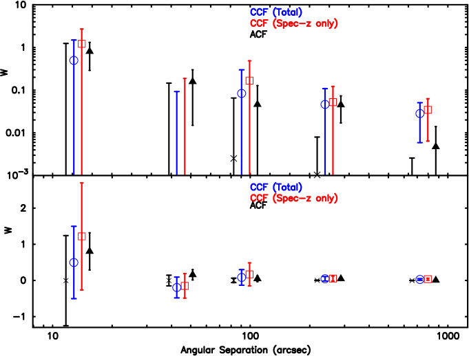
Figure 7.— Two-point angular quasar-LBG CCF (red open squares and blue open circles), the random-LBG CCF (black crosses), and the LBG ACF (filled black triangles) at $z\sim 4$ in the COSMOS field. Top and bottom panel shows the two-point angular quasar-LBG CCF and the LBG ACF in double-logarithmic and semilogarithmic graph, respectively. The data are shown with slight shifts in the horizontal direction for clarity.

Table 2Summary of the $\omega_{\rm QL}$ at $z\sim 4$

$\theta$		$\omega_{\rm QL}$	$\sigma_{\omega_{\rm QL}}$	$D_{\rm Q}D_{\rm L}(\theta)$	$\omega_{\rm QL}$	$\sigma_{\omega_{\rm QL}}$	$D_{\rm Q}D_{\rm L}(\theta)$
(arcsec)		(Total)	(Total)	(Total)	($z_{\rm sp}$ only)	($z_{\rm sp}$ only)	($z_{\rm sp}$ only)
14		0.4970	0.9997	2	1.2178	1.4805	2
46		$-0.1950$	0.2877	9	$-0.1506$	0.3389	6
99		0.0838	0.2156	32	0.1674	0.3189	22
262		0.0463	0.0625	382	0.0523	0.0693	242
792		0.0284	0.0225	2803	0.0347	0.0282	1832

Table 3Summary of the quasar-lbg ccf

$N_{\rm Q}$	$N_{\rm LBG}$	QSO Magnitude	LBG Magnitude	Redshift	$A^{\rm CCF}_{w}$	$A_{w}$	$A_{w}$	$r_{0}$
							($86\%$ upper limit)	($h^{-1}$ Mpc)
16a	835	$-24.0<M_{\rm 1450}<-22.0$	$z^{\prime}<25.0$	$3.1<z<4.5$	3.33${}^{+3.06}_{-1.60}$	3.43${}^{+3.16}_{-1.64}$	$<6.59$	$<10.72$
25b	835	$-24.0<M_{\rm 1450}<-22.0$	$z^{\prime}<25.0$	$3.1<z<4.5$	1.77${}^{+1.66}_{-0.86}$	1.82${}^{+1.71}_{-0.88}$	$<3.53$	$<7.60$

^aNumber of the spectroscopically confirmed quasars.
^bTotal number of the quasars.

Table 4Summary of the $\omega_{\rm LL}$ at $z\sim 4$

$\theta$		$\omega_{\rm LL}$	$\sigma_{\omega_{\rm LL}}$	$D_{\rm L}D_{\rm L}(\theta)$
(arcsec)
14		0.8034	0.5134	40
46		0.1576	0.1426	220
99		0.0463	0.0816	512
262		0.0452	0.0280	5851
792		0.0047	0.0093	42091

3.2. LBG Two-Point Angular Auto-Correlation Function at $z\sim 4$

To constrain the quasar triggering mechanism, we have to calculate the CCF and the LBG two-point angular auto-correlation function (ACF). Since we have calculated the CCF in Section 3.1, we calculate the LBG ACF at $z\sim 4$ in Section 3.2. In order to calculate the LBG two-point angular ACF at $z\sim 4$, we use the Landy & Szalay (1993) estimator:

$$\rm\omega_{\rm LL}(\theta)=\frac{\it\langle DD\rangle-\rm 2\langle\it DR\rangle+\langle RR\rangle}{\it\langle RR\rangle},$$ (19)

where $\langle DD\rangle$, $\langle DR\rangle$, and $\langle RR\rangle$ are the normalized data-data, data-random, and random-random number of pairs. Those are defined as follows:

$$\langle DD\rangle=\frac{D_{\rm L}D_{\rm L}(\theta)}{\it N_{\rm L}(\it N_{\rm L}\rm-1)/2},$$ (20)

$$\langle DR\rangle=\frac{D_{L}R(\theta)}{\it N_{\rm L}\it N_{\rm R}},$$ (21)

and,

$$\langle RR\rangle=\frac{RR(\theta)}{\it N_{\rm R}(\it N_{\rm R}-\rm 1)/2},$$ (22)

where $D_{L}D_{L}(\theta)$, $D_{L}R(\theta)$, and $RR(\theta)$ are number of data-data, data-random, and random-random pairs at angular separation $\theta\pm\Delta\theta$, respectively. In equations (20)–(22), $N_{\rm L}$ and $N_{\rm R}$ are the total number of data in the LBG and random sample, respectively. Using 100,000 random samples which are avoiding the masked regions, we calculate the two-point ACF of LBGs. The obtained results are shown in Figure 7 and Table 4. We find that the quasar-LBG two-point CCF is similar with the LBG two-point ACF at $z\sim 4$. The observed two-point angular ACF is also approximated by a power law form at large scales as follows:

$$\omega_{\rm LL}(\theta)=A_{\omega}^{\rm ACF}(\theta^{-\beta}-\rm C),$$ (23)

where $\beta$ is fixed to be 0.8 (Francke et al. 2008) and C (which gives a value of C = 0.00601 in this case) is the integral constraint. To avoid the one-halo term, we do not use $\rm\omega_{\rm LL}(\theta)$ on small scales ($\rm angular\ separation<40$ arcsec) to calculate $A_{\omega}^{\rm ACF}$. We calculate the correlation amplitude of the LBG ACF, $A_{\omega}^{\rm ACF}$ using equations (16) and (23). As a result, $A_{\omega}^{\rm ACF}$ is $3.65^{+2.23}_{-1.38}$. In addition, we calculate the correlation amplitude for ACF, $A_{\omega}$ (ACF) as follows:

$$A_{\omega}(\rm ACF)=\it\frac{A_{\omega}^{\rm ACF}}{(\rm 1-\it f_{\rm c})^{\rm 2}},$$ (24)

the calculated $A_{\omega}(\rm ACF)$ is 3.88${}^{+2.37}_{-1.47}$. These results are listed in Table 5.

Table 5Summary of the LBG ACF

$N_{\rm LBG}$	LBG Magnitude	Redshift	$A^{\rm ACF}_{w}$	$A_{w}$	$r_{0}$
					($h^{-1}$ Mpc)
835	$z^{\prime}<25.0$	$3.1<z<4.5$	$3.65^{+2.23}_{-1.38}$	$3.88^{+2.37}_{-1.47}$	$6.52^{+3.16}_{-1.96}$

Table 6Summary of the bias factor

$N_{\rm Q}$	$N_{\rm LBG}$		QSO Magnitude	LBG Magnitude	Redshift	$b_{\rm QSO}$	$b_{\rm LBG}$	$b_{\rm QL}$
16	835		$-24.0<M_{\rm 1450}<-22.0$	$z^{\prime}<25.0$	$3.1<z<4.5$	$<10.50$	$4.92^{+2.07}_{-1.29}$	$<7.69$
25	835		$-24.0<M_{\rm 1450}<-22.0$	$z^{\prime}<25.0$	$3.1<z<4.5$	$<5.63$	$4.92^{+2.07}_{-1.29}$	$<5.65$

3.3. The Spatial Correlation Function

In order to calculate the bias factor for LBGs and low-luminosity quasars, we calculate the spatial correlation function for the ACF and CCF. The spatial correlation function is given as follows:

$$\xi(r)=(r/r_{\rm 0})^{-\gamma},$$ (25)

where $r_{\rm 0}$ is the spatial correlation length and $\gamma$ = $\beta$+1. The spatial correlation function for the ACF is calculated with the following relation (Totsuji & Kihara 1969),

$$A_{w}(\rm ACF)=\it\frac{H_{\gamma}r_{\rm 0}^{\gamma}\int F(z)r^{\rm 1-\it\gamma}_{c}(z)N_{\rm g}^{\rm 2}\it(z)E(z)dz}{(c/H_{\rm 0})[\int N_{\rm g}(z)dz]^{\rm 2}},$$ (26)

where $r_{c}$ is the comoving radial distance, $N_{\rm g}(z)$ is the redshift distribution of LBGs, and $F(z)$ is the evolution of clustering with redshift, which is assumed to be negligible and is set equal to 1 in this paper. In equation (26), $H_{\gamma}$ and $E(z)$ are calculated as follows:

$$H_{\gamma}=\Gamma(1/2)\frac{\Gamma[(\gamma-1)/2]}{\Gamma(\gamma/2)},$$ (27)

and,

$$E(z)=[\Omega_{m}(1+z)^{3}+\Omega_{\Lambda}]^{1/2}.$$ (28)

The spatial correlation function for the CCF is also calculated following the relation (Croom & Shanks 1999);

$$A_{w}(\rm CCF)=\it\frac{H_{\gamma}r_{\rm 0}^{\gamma}\int F(z)r^{\rm 1-\it\gamma}_{c}(z)N_{\rm g}\it(z)N_{\rm q}\it(z)E(z)dz}{(c/H_{\rm 0})[\int N_{\rm g}\it(z)dz\int N_{\rm q}\it(z)dz]},$$ (29)

where $N_{\rm q}(z)$ is the redshift distributions of quasars. We calculate the spatial correlation lengths of the LBG ACF and the quasar-LBG CCF using these equations. As a result, the spatial correlation length for the LBG ACF is 6.52${}^{+3.16}_{-1.96}$ $h^{-1}$ Mpc. The $86\%$ upper limits of the spatial correlation lengths for the quasar-LBG CCF are $7.60$ $h^{-1}$ Mpc and $10.72$ $h^{-1}$ Mpc for the total and the spectroscopic sample, respectively. These results are also summarized in Tables 3 and 5.

3.4. The Bias Factor

We now investigate the bias factor for low-luminosity quasars at $z\sim 4$ in the COSMOS field to study the luminosity dependence of the quasar clustering and constrain the triggering mechanism of the quasar activity. In order to investigate the quasar bias factor, we have to estimate the galaxy bias at the same redshift. In this paper, we estimate the galaxy bias factor at the same redshift using LBGs. The bias factors for LBGs and quasars are defined as follows:

$$b_{\rm LBG}(z)=\sqrt[]{\frac{\xi_{\rm L}(8,z)}{\xi_{\rm DM}(8,z)}},b_{\rm QSO}(z)=\sqrt[]{\frac{\xi_{\rm Q}(8,z)}{\xi_{\rm DM}(8,z)}},$$ (30)

where $\xi_{\rm L}(8,z)$ = $(r_{\rm 0}(z)/8)^{\gamma}$, $\xi_{\rm Q}(8,z)$ = $(r_{\rm 0}(z)/8)^{\gamma}$, and $\xi_{\rm DM}(8,z)$ are the spatial correlation functions of LBGs, quasars, and dark matter halos evaluated at 8 $h^{-1}$ Mpc, respectively. The correlation function of dark matter halos is as follows (Peebles 1980):

$$\xi_{\rm DM}(8,z)=\frac{\sigma^{2}_{8}(z)}{J_{2}},$$ (31)

where $J_{2}$ = $72/[(3-\gamma)(4-\gamma)(6-\gamma)2^{\gamma}]$ and $\sigma^{2}_{8}(z)$ is the dark matter density variance in a sphere with a comoving radius of 8 $h^{-1}$ Mpc. We calculate $\sigma_{8}(z)$ using the following equation:

$$\sigma_{8}(z)=\sigma_{8}\frac{D(z)}{D(0)},$$ (32)

where $D(z)$ is the linear growth factor scaled to unity at the present time and we calculate it as follows (Myers et al. 2006):

$$D(z)=\frac{g_{z}}{g_{\rm 0}}\frac{1}{(1+z)}.$$ (33)

We calculate $g_{z}$ by using the following equation (Carroll et al. 1992; Myers et al. 2006):

$$g_{z}=\frac{5\Omega_{mz}}{2}\Bigl{[}\Omega^{4/7}_{mz}-\Omega_{\Lambda z}+(1+\frac{\Omega_{mz}}{2})(1+\frac{\Omega_{\Lambda z}}{70})\Bigl{]}^{-1},$$ (34)

where we also calculate $\Omega_{mz}$ and $\Omega_{\Lambda z}$ as follows (Myers et al. 2006):

$$\Omega_{mz}=\Bigl{(}\frac{H_{\rm 0}}{H_{z}}\Bigl{)}^{2}\Omega_{m}(1+z)^{3},\Omega_{\Lambda z}=\Bigl{(}\frac{H_{\rm 0}}{H_{z}}\Bigl{)}^{2}\Omega_{\Lambda},$$ (35)

where $H_{z}$ is expressed as follows (Myers et al. 2006):

$$H_{z}=H_{\rm 0}[\Omega_{m}(1+z)^{3}+\Omega_{\Lambda}]^{1/2}.$$ (36)

Using equations (30)–(36), we calculate the correlation function of the dark matter halos evaluated at 8 $h^{-1}$ Mpc and the bias factor for LBGs. As a result, the bias factor for the LBGs is 4.92${}^{+2.07}_{-1.29}$. Next we describe how to calculate the bias factor for low-luminosity quasars at $z\sim 4$ using the bias factor for LBGs. In order to calculate the bias factor for low-luminosity quasars, we use the relations as follows (Mountrichas et al. 2009):

$$b^{2}_{\rm LBG}=\sigma^{2}_{\rm 8,LBG}/\sigma^{2}_{\rm 8,DM},\ b_{\rm QSO}b_{\rm LBG}=b_{\rm QL}^{2},$$ (37)

where $b_{\rm QL}$ is the bias factor for the quasar-LBG CCF and this is calculated as follows:

$$b_{\rm QL}^{2}=\sigma^{2}_{\rm 8,QSO-LBG}/\sigma^{2}_{\rm 8,DM}.$$ (38)

We then obtain the $86\%$ upper limits of $b_{\rm QL}$ $=5.65$ and $7.69$ for the total and the spectroscopic sample, respectively. Based on these values, we derive the $86\%$ upper limits of $b_{\rm QSO}$ $=5.63$ and $10.50$ for the total and spectroscopic sample, respectively. The results of the bias factors for $b_{\rm LBG}$, $b_{\rm QL}$, and $b_{\rm QSO}$ are summarized in Table 6.

3.5. The Typical Dark Matter Halo Mass

The inferred bias factor for low-luminosity quasars can be used to calculate the typical dark matter halo mass ($M_{\rm DM}$). To calculate the typical dark matter halo mass in which low-luminosity quasars at $z\sim 4$ reside, we use Equation (8) of Sheth et al. (2001) with parameters which are recalibrated by Tinker et al. (2005) as follows:

$$b(M,z)=1+\frac{1}{\sqrt{a}\delta_{c}}\Bigl{[}a\nu^{2}\sqrt{a}+b\sqrt{a}(a\nu^{2})^{(1-c)}$$

$$-\frac{(a\nu^{2})^{c}}{(a\nu^{2})^{c}+b(1-c)(1-c/2)}\Bigl{]},$$ (39)

where $\nu=\frac{\delta_{c}}{\sigma(m)D(z)}$, $a=0.707$, $b=0.35$, $c=0.80$, and $\delta_{c}\sim 1.686$ is the critical overdensity. $\sigma(M)$ is the linear theory rms mass fluctuation on the mass scale $M$ and we calculate it using equations (A8), (A9), and (A10) of van den Bosch (2002). The dark matter halo mass can be estimated more accurately by utilizing the halo occupation distribution (HOD) models. However the errors in the derived quasar bias are still large and therefore we only use Equation (39). We then obtain the $86\%$ upper limits of log $(M_{\rm DM}/(h^{-1}M_{\odot}))=12.7$ and $13.5$, for the total and the spectroscopic sample, respectively.

Figure 8.— Bias factor for LBGs as a function of UV magnitude. Star, square, open circle, triangle, and solid circle points show our result, results of Hildebrandt et al. (2009), Ouchi et al. (2004), Allen et al. (2005), and Ouchi et al. (2001), respectively.

Table 7Summary of the reported bias factor for quasars

Sample			$N_{\rm Q}$	Quasar (AGN) Luminosity	$z$-Range	Quasar (AGN) Bias	Type of CF	Reference
				(mag or erg s-1)
COSMOS			16	$-24.0<M_{\rm 1450}<-22.0$	$3.1<z<4.5$	$<10.50$	CCF	This work
COSMOS			25	$-24.0<M_{\rm 1450}<-22.0$	$3.1<z<4.5$	$<5.63$	CCF	This work
GOODSa			$25$	$-30<M_{\rm UV}<-25$	$1.6<z<3.7$	$3.9\pm 3.0^{b}$	CCF	Adelberger & Steidel (2005)
GOODS			$54$	$-25<M_{\rm UV}<-20$	$1.6<z<3.7$	$4.7\pm 1.7^{b}$	CCF	Adelberger & Steidel (2005)
2QZc			18,066	$18.25<b_{J}<20.85$	$0.3<z<2.2$	$2.02\pm 0.07$	ACF	Croom et al. (2005)
2QZ			$\sim 14,000$d	$M_{b_{J}}<-22.5$e	$0.80<z<1.06$	$1.57^{+0.30}_{-0.37}$	ACF	Porciani & Norberg (2006)
2QZ			$\sim 14,000$d	$M_{b_{J}}<-22.5$e	$1.06<z<1.30$	$1.76^{+0.35}_{-0.43}$	ACF	Porciani & Norberg (2006)
2QZ			$\sim 14,000$d	$M_{b_{J}}<-22.5$ e	$1.30<z<1.51$	$2.13^{+0.29}_{-0.33}$	ACF	Porciani & Norberg (2006)
2QZ			$\sim 14,000$d	$M_{b_{J}}<-22.5$e	$1.51<z<1.70$	$2.33^{+0.33}_{-0.39}$	ACF	Porciani & Norberg (2006)
2QZ			$\sim 14,000$d	$M_{b_{J}}<-22.5$ e	$1.70<z<1.89$	$3.02^{+0.45}_{-0.53}$	ACF	Porciani & Norberg (2006)
2QZ			$\sim 14,000$d	$M_{b_{J}}<-22.5$e	$1.89<z<2.10$	$4.13^{+0.49}_{-0.55}$	ACF	Porciani & Norberg (2006)
SDSS DR1			$100,563^{d}$	$14.5\leq g<21.0$	$0.4<z<1.0$	$1.34\pm 0.56$	ACF	Myers et al. (2006)
SDSS DR1			$100,563^{d}$	$14.5\leq g<21.0$	$1.0<z<1.4$	$2.20\pm 0.26$	ACF	Myers et al. (2006)
SDSS DR1			$100,563^{d}$	$14.5\leq g<21.0$	$1.4<z<1.7$	$2.58\pm 0.35$	ACF	Myers et al. (2006)
SDSS DR1			$100,563^{d}$	$14.5\leq g<21.0$	$1.7<z<2.1$	$2.42\pm 0.39$	ACF	Myers et al. (2006)
SDSS DR1			$100,563^{d}$	$14.5\leq g<21.0$	$2.1<z<2.8$	$3.12\pm 0.80$	ACF	Myers et al. (2006)
$\rm 2QZ+2SLAQ$f			$22,416$g	$18.25<b_{J}<20.85^{h}$	$0.3<z<2.9$	$1.5\pm 0.2$	ACF	da Ângela et al. (2008)
			$6,374$i	$20.50<g<21.85^{j}$
MUSYC ECDF$-$Sk			58	$R<25.5$	$2.7<z<3.8$	$5.5\pm 2.0$	CCF	Francke et al. (2008)
AEIGSl			113	$M_{B}$ $=-20.98$ (median)	$0.7<z<1.4$	$1.48\pm 0.12$	CCF	Coil et al. (2009)
XMM$-$COSMOSm			538	$i^{\prime}<23.0$	$0.2<z<3.0$	$2.0\pm 0.2$	ACF	Gilli et al. (2009)
2SLAQ			$503$	$18.00\leq g\leq 21.85$	$0.35\leq z\leq 0.75$	$1.84\pm 0.3$	CCF	Mountrichas et al. (2009)
SDSS DR5			$2,476$	$i\leq 19.1$	$0.25<z<0.60$	$1.09\pm 0.15$	CCF	Padmanabhan et al. (2009)
SDSS DR5			30,239	$M_{i}<-22$	$0.3\leq z\leq 2.2$	$2.06\pm 0.03$	ACF	Ross et al. (2009)
SDSS DR5			7,902	$M_{i}<-22$	$0.1<z<0.8$	$1.32\pm 0.17$	ACF	Shen et al. (2009)
SDSS DR5			9,975	$M_{i}<-22$	$0.8<z<1.4$	$2.31\pm 0.22$	ACF	Shen et al. (2009)
SDSS DR5			11,304	$M_{i}<-22$	$1.4<z<2.0$	$2.96\pm 0.26$	ACF	Shen et al. (2009)
SDSS DR5			3,828	$M_{i}<-22$	$2.0<z<2.5$	$4.69\pm 0.70$	ACF	Shen et al. (2009)
SDSS DR5			2,693	$M_{i}<-22$	$2.9<z<3.5$	$7.76\pm 1.44$	ACF	Shen et al. (2009)
SDSS DR5			1,788	$M_{i}<-22$	$3.5<z<5.0$	$12.96\pm 2.09$	ACF	Shen et al. (2009)
SDSS DR5			1,788	$M_{i}<-22$	$3.5<z<5.0$	$9.85\pm 2.27$	ACF	Shen et al. (2009)
SDSS DR7			37,290	$i\leq 19.1$	$0.8\leq z\leq 2.2$	$1.50\pm 0.37$	ACF	Ivashchenko et al. (2010)
Bo$\ddot{o}$tesn			445	log $L_{\rm bol}$ $=45.86$ (median)	$0.7<z<1.8$	$2.17\pm 0.55$	CCF	Hickox et al. (2011)
Bo$\ddot{o}$tes			445	log $L_{\rm bol}$ $=45.86$ (median)	$0.7<z<1.8$	$2.50\pm 0.65$	ACF	Hickox et al. (2011)
RASSo			1,552	$43.7<$ log $L_{\rm X}$ (0.1$-$2.4keV) $<$44.7	$0.16<z<0.36$	$1.30\pm 0.09$	CCF	Miyaji et al. (2011)
RASS			$629$	$43.05\lesssim$ log $L_{\rm X}$ (0.1$-$2.4keV) $\lesssim 44.12$	$0.07<z<0.16$	$1.19^{+0.08}_{-0.09}$	ACF	Krumpe et al. (2012)
RASS			$1,552$	$43.69\lesssim$ log $L_{\rm X}$ (0.1$-$2.4keV) $\lesssim 44.68$	$0.16<z<0.36$	$1.06^{+0.09}_{-0.11}$	ACF	Krumpe et al. (2012)
RASS			$876$	$44.25\lesssim$ log $L_{\rm X}$ (0.1$-$2.4keV) $\lesssim 45.04$	$0.36<z<0.50$	$0.96^{+0.22}_{-0.54}$	ACF	Krumpe et al. (2012)
XMM/SDSS			297	$41.0<$ log $L_{X}$ (2$-$10keV) $<44.0$	$0.03<z<0.2$	$1.23^{+0.12}_{-0.17}$	CCF	Mountrichas & Georgakakis (2012)
$\rm Many^{p}$			1,466	log $L_{\rm X}$ (0.5$-$8keV) $\geq 41.0$	$0<z<3.0$	$2.26\pm 0.16$	ACF	Koutoulidis et al. (2013)
SDSS DR7			8,198	$-28.693<M_{i^{\prime}}<-22.576$	$0.3<z<0.9$	$1.38\pm 0.10$	CCF	Shen et al. (2013)

^aThe Great Observatories Origins Deep Survey (GOODS; Dickinson et al. 2003).
^bThe bias factors for quasars which are derived by Francke et al. (2008).
^cThe 2dF QSO Redshift Survey (2QZ; Boyle et al. 2000).
^dThe total numbers of quasars at $0.80<z<2.10$ (Porciani & Norberg 2006).
^eThe absolute magnitude range of quasars at $0.80<z<2.10$ (Porciani & Norberg 2006).
^fThe 2dF-SDSS LRG and QSO (2SLAQ; Cannon et al. 2006; Croom et al. 2009b).
^gThe number of 2QZ quasar sample.
^hThe magnitude range of 2QZ quasar sample.
ⁱThe number of 2SLAQ quasar sample.
^jThe magnitude range of 2SLAQ quasar sample.
^kThe Multiwavelength Survey by Yale-Chile (MUSYC; Gawiser et al. 2006) Extended Chandra Deep Field-South (ECDF-S; Lehmer et al. 2005; Virani et al. 2006).
^lAll-Wavelength Extended Groth Strip International Survey (AEGIS; Davis et al. 2007).
^mXMM-Newton wide-field survey in the COSMOS field (XMM-COSMOS; Hasinger et al. 2007; Cappelluti et al. 2007).
ⁿBo$\ddot{o}$tes multiwavelength survey (Bo$\ddot{o}$tes; Hickox et al. 2007).
^oThe ROSAT All Sky Survey (RASS; Voges et al. 1999).
^pChandra Deep Field (CDF)-North, CDF-South, AEIGS, COSMOS, and Extend CDF-South.

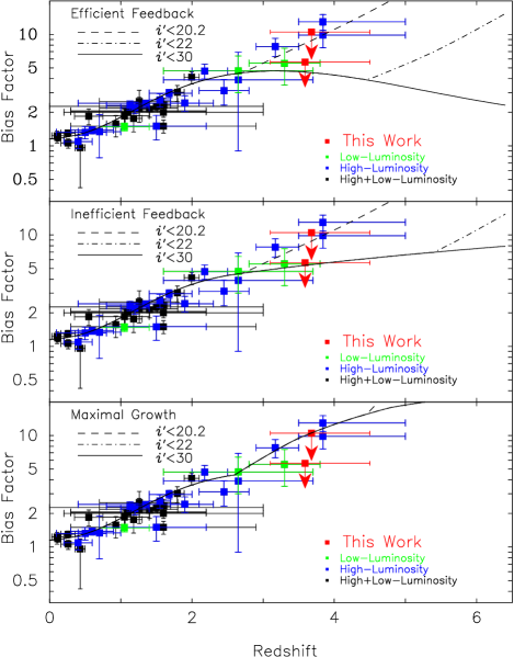
Figure 9.— Quasar bias factor as a function of redshift. Red, green, blue and black squares show the bias factors for our results (total and spectroscopic sample), low-luminosity quasars ($M_{\rm 1450}>-24$), high-luminosity quasars ($M_{\rm 1450}<-24$), and high+low-luminosity quasars, respectively. Black lines show the quasar bias factors as a function of redshift with three different models. The model shown in the top panel assumes that SMBH growth shuts down after quasar phase (efficient feedback). The model shown in the middle panel assumes that all $z>2$ black holes grow with the observed quasar luminosity function to the characteristic peak luminosities at $z\sim 2$, then shut down (inefficient feedback). The model shown in the bottom panel assumes that quasar growth tracks host halo growth, even after a quasar episode, until $z=2$ (maximal growth). Dashed, Dash-dotted, and solid lines in each panel show the $i^{\prime}$-band magnitude ranges at $i^{\prime}<20.2$, $i^{\prime}<22$, and $i^{\prime}<30$, respectively (Hopkins et al. 2007).

4. Discussion

We calculated the quasar-LBG two-point CCF and the LBG ACF at $z\sim 4$ to investigate the luminosity dependence of quasar clustering and constrain the dark matter halo mass in which low-luminosity quasars at $z\sim 4$ reside. Since the LBG ACF at $z\sim 4$ has been studied by many investigators (Ouchi et al. 2001, 2004, 2005; Allen et al. 2005; Kashikawa et al. 2006; Lee et al. 2006; Hildebrandt et al. 2009; Savoy et al. 2011; Barone-Nugent et al. 2014), we compare the previous results of $b_{\rm LBG}$ with the derived $b_{\rm LBG}$ in this work (Figure 8). Our inferred bias factor for LBGs ($b_{\rm LBG}$ is $4.92^{+2.07}_{-1.29}$ at $M_{\rm UV}<-20.9$) is not inconsistent with the luminosity dependence of the galaxies bias factor which are reported from previous studies. We also found that the quasar-LBG CCF shows similar clustering with the LBG ACF while the errors of our results are large, due to the low numbers of low-luminosity quasars.

To constrain the triggering mechanism of the activity in low-luminosity quasars at $z\sim 4$, we calculated the bias factor for low-luminosity quasars in the COSMOS field, which are fainter than the characteristic absolute magnitude. The $86\%$ upper limits of bias factors of $z\sim 4$ low-luminosity quasars are $5.63$ and $10.50$ for the total and the spectroscopic samples, respectively. The inferred bias factor for the total sample is smaller than that for the spectroscopic sample, while both results are just the $86\%$ upper limits. In order to clarify the accurate bias factor for low-luminosity quasars, we need larger samples of low-luminosity quasars.

The bias factors for low-luminosity quasars derived in this work and results for different redshift and/or luminosity given in previous studies (Adelberger & Steidel 2005; Croom et al. 2005; Myers et al. 2006; Porciani & Norberg 2006; da Ângela et al. 2008; Francke et al. 2008; Gilli et al. 2009; Shen et al. 2009; Ross et al. 2009; Coil et al. 2009; Mountrichas et al. 2009; Padmanabhan et al. 2009; Ivachenko et al. 2010; Hickox et al. 2011; Miyaji et al. 2011; Krumpe et al. 2012; Mountrichas & Georgakakis 2012; Koutoulidis et al. 2013) are showed in Figure 9. We also summarized our result and the previous results of the bias factor for quasars in Table 7. The bias factors which are plotted in Figure 9 and Table 7 are showing results calculated by the ACF or CCF. In order to study the redshift dependence of the bias factor for low-luminosity quasars from $z\sim 3$ to $z\sim 4$, we compare previous results at $z\sim 3$ with our result at $z\sim 4$. Francke et al. (2008) calculated the bias factor for AGNs at $z\sim 3$ at the UV magnitude range between $-26$ and $-20$ and the obtained bias factor is $5.5\pm 2$. Our result for the total sample is consistent with that of their study, though we can not rule out the possibility of a lower value of the bias factor for low-luminosity quasars. We also compare the bias factor for luminous quasars which are brighter than the characteristic absolute magnitude at a similar redshift (Shen et al. 2009). Shen et al. (2009) calculated the bias factor for luminous quasars at $3.5<z<5.0$ and the obtained bias factors are 12.96$\pm 2.09$ (excluding negative data points of the correlation function) and 9.85$\pm 2.27$ (including negative data points of the correlation function), respectively. Our result for spectroscopic sample is consistent with their study, though we can not rule out the possibility of a lower value of the bias factor for low-luminosity quasars. Our result for total sample is much smaller than that of Shen et al. (2009). The $86\%$ upper limits of the inferred bias factors for low-luminosity quasars at $z\sim 4$ correspond to the typical dark matter halo mass are log $(M_{\rm DM}/(h^{-1}M_{\odot}))=12.7$ and $13.5$ for the total and the spectroscopic samples, respectively. This result is not inconsistent with the predicted bias for quasars which is estimated by the major merger models (e.g., Hopkins et al. 2007).

Hopkins et al. (2007) predicted the bias factors as a function of redshift using three different models. The first one is that SMBH growth shuts down after each quasar phase (efficient feedback). This model is assuming that each SMBH only experiences one phase of quasar activity and SMBH growth will stop after this one quasar phase. The second one is that all SMBHs at $z>2$ grow with the QLF to the characteristic peak luminosities at $z\sim 2$ and after that SMBH growth shut down (inefficient feedback). This model is assuming that $z\sim 6$ quasars grow either continuously or episodically with their host systems until $z\sim 2$. Hence a quasar feedback at $z>2$ is insufficient to shut down a quasar. The last one is that SMBH growth with a Eddington rate until $z=2$ (maximal growth). This model is assuming that SMBHs will grow at their Eddington rate until $z\sim 2$. In case of efficient feedback and inefficient feedback model, they predict that the bias factor for low-luminosity quasars becomes weak with decreasing UV luminosity. In contrast, Incase of the maximal growth model, this predict that the luminosity dependence of the quasar bias is not detected. Our result for total sample is lower than that of the maximal growth model. However those three models cannot be discriminated by our result for spectroscopic sample. While we can also constrain the quasar lifetime using the quasar bias factor and quasar space density in principle, it is currently too challenging to constrain it due to the lack of the spectroscopic sample of low-luminosity quasars. In order to measure the bias factor for low-luminosity quasars with smaller error bars, we need to use larger samples of low-luminosity quasars. Further observations of low-luminosity quasars in a wider survey area are crucial to provide firm constraints on different scenarios of quasar evolution and elucidate the triggering mechanism of low-luminosity quasars, especially at $z>3$, with smaller statistical errors. Surveys for high-$z$ low-luminosity quasars with the next-generation wide-field prime-focus camera for the Subaru Telescope (Hyper Suprime-Cam: Miyazaki et al. 2006, 2012), Euclid (Laureijs et al. 2011), and the Large Synoptic Survey Telescope (Ivezic et al. 2008) will address these issues in the very near future.

5. Summary

We have estimated the quasar-LBG two-point CCF for low-luminosity ($-24<M_{\rm 1450}<-22$) quasars and LBGs at $3.1<z<4.5$ in the COSMOS field. Our quasar sample consists of 25 quasars with spectroscopic or photometric redshifts. This sample is referred as the total sample. We also use the 16 quasars with spectroscopic redshifts (the spectroscopic sample). We use a sample of 835 LBGs with $z^{\prime}<25.0$ in the same redshift range. We have also estimated the LBG ACF at $z\sim 4$ for comparison with the quasar-LBG CCF at $z\sim 4$. Our main results are summarized below.

1. The correlation amplitudes of the quasar-LBG CCF are $1.82^{+1.71}_{-0.88}$ and 3.43${}^{+3.16}_{-1.64}$ for the total and the spectroscopic sample, respectively. The correlation amplitude of the LBG ACF is 3.88${}^{+2.37}_{-1.47}$.

2. The $86\%$ upper limits of the spatial correlation lengths for the quasar-LBG CCF are $7.60$ $h^{-1}$ Mpc and $10.72$ $h^{-1}$ Mpc for the total and the spectroscopic sample, respectively. The spatial correlation length for the LBG ACF is 6.52${}^{+3.16}_{-1.96}$ $h^{-1}$ Mpc.

3. The $86\%$ upper limits of the bias factors of $z\sim 4$ low-luminosity quasars are $5.63$ and $10.50$ for the total and the spectroscopic sample, respectively. The bias factor for the LBGs is 4.92${}^{+2.07}_{-1.29}$.

4. We find that the bias factor for spectroscopic confirmed low-luminosity quasars at $z\sim 4$ is consistent with the bias factor for luminous quasars at $z\sim 4$, though we can not rule out the possibility of a lower value of the bias factor for low-luminosity quasars.

5. We also find that the bias factor for low-luminosity quasars at $z\sim 4$ is consistent with that of previous results at $z\sim 3$ at similar quasar luminosity, though we can not rule out the possibility of a lower value of the bias factor for low-luminosity quasars.

6. The $86\%$ upper limits of the inferred dark matter halo masses are log $(M_{\rm DM}/(h^{-1}M_{\odot}))=12.7$ and $13.5$ for the total and the spectroscopic sample, respectively. This result is not inconsistent with the predicted bias for quasars which is estimated by the major merger models.
   

More specific constraints on SMBH growth scenarios will be obtained through larger samples of low-luminosity quasars at high redshifts that will be discovered by forthcoming wider and deeper quasar surveys.

References

- Adelberger & Steidel (2005) Adelberger, K. L., & Steidel, C. C. 2005, ApJ, 627, L1
- Allen et al. (2005) Allen, P. D., Moustakas, L. A., Dalton, G., et al. 2005, MNRAS, 360, 1244
- Allevato et al. (2011) Allevato, V., Finoguenov, A., Cappelluti, N., et al. 2011, ApJ, 736, 99
- Allevato et al. (2014) Allevato, V., Finoguenov, A., Civano, F., et al. 2014, ApJ, 796, 4
- Barone-Nugent et al. (2014) Barone-Nugent, R. L., Trenti, M., Wyithe, J. S. B., et al. 2014, ArXiv e-prints
- Bielby et al. (2011) Bielby, R. M., Shanks, T., Weilbacher, P. M., et al. 2011, MNRAS, 414, 2
- Boulade et al. (2003) Boulade, O., Charlot, X., Abbon, P., et al. 2003, in Society of Photo-Optical Instrumentation Engineers (SPIE) Conference Series, Vol. 4841, Society of Photo-Optical Instrumentation Engineers (SPIE) Conference Series, ed. M. Iye & A. F. M. Moorwood, 72–81
- Bouwens et al. (2007) Bouwens, R. J., Illingworth, G. D., Franx, M., & Ford, H. 2007, ApJ, 670, 928
- Boyle et al. (2000) Boyle, B. J., Shanks, T., Croom, S. M., et al. 2000, MNRAS, 317, 1014
- Bruzual & Charlot (2003) Bruzual, G., & Charlot, S. 2003, MNRAS, 344, 1000
- Cannon et al. (2006) Cannon, R., Drinkwater, M., Edge, A., et al. 2006, MNRAS, 372, 425
- Capak et al. (2007) Capak, P., Aussel, H., Ajiki, M., et al. 2007, ApJS, 172, 99
- Cappelluti et al. (2007) Cappelluti, N., Hasinger, G., Brusa, M., et al. 2007, ApJS, 172, 341
- Cardamone et al. (2010) Cardamone, C. N., van Dokkum, P. G., Urry, C. M., et al. 2010, ApJS, 189, 270
- Carroll et al. (1992) Carroll, S. M., Press, W. H., & Turner, E. L. 1992, ARA&A, 30, 499
- Coil et al. (2009) Coil, A. L., Georgakakis, A., Newman, J. A., et al. 2009, ApJ, 701, 1484
- Croft et al. (1999) Croft, R. A. C., Dalton, G. B., & Efstathiou, G. 1999, MNRAS, 305, 547
- Croom & Shanks (1999) Croom, S. M., & Shanks, T. 1999, MNRAS, 303, 411
- Croom et al. (2005) Croom, S. M., Boyle, B. J., Shanks, T., et al. 2005, MNRAS, 356, 415
- Croom et al. (2009a) Croom, S. M., Richards, G. T., Shanks, T., et al. 2009a, MNRAS, 399, 1755
- Croom et al. (2009b) —. 2009b, MNRAS, 392, 19
- da Ângela et al. (2008) da Ângela, J., Shanks, T., Croom, S. M., et al. 2008, MNRAS, 383, 565
- Davis et al. (2007) Davis, M., Guhathakurta, P., Konidaris, N. P., et al. 2007, ApJ, 660, L1
- Dickinson et al. (2003) Dickinson, M., Giavalisco, M., & GOODS Team. 2003, in The Mass of Galaxies at Low and High Redshift, ed. R. Bender & A. Renzini, 324
- Francke et al. (2008) Francke, H., Gawiser, E., Lira, P., et al. 2008, ApJ, 673, L13
- Gawiser et al. (2006) Gawiser, E., van Dokkum, P. G., Herrera, D., et al. 2006, ApJS, 162, 1
- Gilli et al. (2009) Gilli, R., Zamorani, G., Miyaji, T., et al. 2009, A&A, 494, 33
- Groth & Peebles (1977) Groth, E. J., & Peebles, P. J. E. 1977, ApJ, 217, 385
- Häring & Rix (2004) Häring, N., & Rix, H.-W. 2004, ApJ, 604, L89
- Hasinger et al. (2007) Hasinger, G., Cappelluti, N., Brunner, H., et al. 2007, ApJS, 172, 29
- Hickox et al. (2007) Hickox, R. C., Jones, C., Forman, W. R., et al. 2007, ApJ, 671, 1365
- Hickox et al. (2011) Hickox, R. C., Myers, A. D., Brodwin, M., et al. 2011, ApJ, 731, 117
- Hildebrandt et al. (2009) Hildebrandt, H., Pielorz, J., Erben, T., et al. 2009, A&A, 498, 725
- Hopkins et al. (2007) Hopkins, P. F., Lidz, A., Hernquist, L., et al. 2007, ApJ, 662, 110
- Husband et al. (2013) Husband, K., Bremer, M. N., Stanway, E. R., et al. 2013, MNRAS, 432, 2869
- Ikeda et al. (2011) Ikeda, H., Nagao, T., Matsuoka, K., et al. 2011, ApJ, 728, L25
- Ikeda et al. (2012) —. 2012, ApJ, 756, 160
- Ilbert et al. (2009) Ilbert, O., Capak, P., Salvato, M., et al. 2009, ApJ, 690, 1236
- Ivashchenko et al. (2010) Ivashchenko, G., Zhdanov, V. I., & Tugay, A. V. 2010, MNRAS, 409, 1691
- Ivezic et al. (2008) Ivezic, Z., Tyson, J. A., Acosta, E., et al. 2008, ArXiv e-prints
- Jones et al. (2012) Jones, T., Stark, D. P., & Ellis, R. S. 2012, ApJ, 751, 51
- Kashikawa et al. (2006) Kashikawa, N., Yoshida, M., Shimasaku, K., et al. 2006, ApJ, 637, 631
- Koekemoer et al. (2007) Koekemoer, A. M., Aussel, H., Calzetti, D., et al. 2007, ApJS, 172, 196
- Komiya et al. (2013) Komiya, Y., Shirasaki, Y., Ohishi, M., & Mizumoto, Y. 2013, ApJ, 775, 43
- Koutoulidis et al. (2013) Koutoulidis, L., Plionis, M., Georgantopoulos, I., & Fanidakis, N. 2013, MNRAS, 428, 1382
- Krolewski & Eisenstein (2015) Krolewski, A. G., & Eisenstein, D. J. 2015, ArXiv e-prints
- Krumpe et al. (2012) Krumpe, M., Miyaji, T., Coil, A. L., & Aceves, H. 2012, ApJ, 746, 1
- Landy & Szalay (1993) Landy, S. D., & Szalay, A. S. 1993, ApJ, 412, 64
- Laureijs et al. (2011) Laureijs, R., Amiaux, J., Arduini, S., et al. 2011, ArXiv e-prints
- Leauthaud et al. (2007) Leauthaud, A., Massey, R., Kneib, J.-P., et al. 2007, ApJS, 172, 219
- Lee et al. (2006) Lee, K.-S., Giavalisco, M., Gnedin, O. Y., et al. 2006, ApJ, 642, 63
- Lehmer et al. (2005) Lehmer, B. D., Brandt, W. N., Alexander, D. M., et al. 2005, ApJS, 161, 21
- Ling et al. (1986) Ling, E. N., Barrow, J. D., & Frenk, C. S. 1986, MNRAS, 223, 21P
- Madau (1995) Madau, P. 1995, ApJ, 441, 18
- Marconi & Hunt (2003) Marconi, A., & Hunt, L. K. 2003, ApJ, 589, L21
- Masters et al. (2012) Masters, D., Capak, P., Salvato, M., et al. 2012, ApJ, 755, 169
- McConnell & Ma (2013) McConnell, N. J., & Ma, C.-P. 2013, ApJ, 764, 184
- McCracken et al. (2012) McCracken, H. J., Milvang-Jensen, B., Dunlop, J., et al. 2012, A&A, 544, A156
- Miyaji et al. (2011) Miyaji, T., Krumpe, M., Coil, A. L., & Aceves, H. 2011, ApJ, 726, 83
- Miyaji et al. (2007) Miyaji, T., Zamorani, G., Cappelluti, N., et al. 2007, ApJS, 172, 396
- Miyazaki et al. (2002) Miyazaki, S., Komiyama, Y., Sekiguchi, M., et al. 2002, PASJ, 54, 833
- Miyazaki et al. (2006) Miyazaki, S., Komiyama, Y., Nakaya, H., et al. 2006, in Society of Photo-Optical Instrumentation Engineers (SPIE) Conference Series, Vol. 6269, Society of Photo-Optical Instrumentation Engineers (SPIE) Conference Series
- Miyazaki et al. (2012) Miyazaki, S., Komiyama, Y., Nakaya, H., et al. 2012, in Society of Photo-Optical Instrumentation Engineers (SPIE) Conference Series, Vol. 8446, Society of Photo-Optical Instrumentation Engineers (SPIE) Conference Series
- Mountrichas & Georgakakis (2012) Mountrichas, G., & Georgakakis, A. 2012, MNRAS, 420, 514
- Mountrichas et al. (2009) Mountrichas, G., Sawangwit, U., Shanks, T., et al. 2009, MNRAS, 394, 2050
- Myers et al. (2007) Myers, A. D., Brunner, R. J., Nichol, R. C., et al. 2007, ApJ, 658, 85
- Myers et al. (2006) Myers, A. D., Brunner, R. J., Richards, G. T., et al. 2006, ApJ, 638, 622
- Ouchi et al. (2001) Ouchi, M., Shimasaku, K., Okamura, S., et al. 2001, ApJ, 558, L83
- Ouchi et al. (2004) —. 2004, ApJ, 611, 685
- Ouchi et al. (2005) Ouchi, M., Hamana, T., Shimasaku, K., et al. 2005, ApJ, 635, L117
- Padmanabhan et al. (2009) Padmanabhan, N., White, M., Norberg, P., & Porciani, C. 2009, MNRAS, 397, 1862
- Peebles (1980) Peebles, P. J. E. 1980, The large-scale structure of the universe
- Pickles (1998) Pickles, A. J. 1998, PASP, 110, 863
- Porciani & Norberg (2006) Porciani, C., & Norberg, P. 2006, MNRAS, 371, 1824
- Rees (1984) Rees, M. J. 1984, ARA&A, 22, 471
- Richards et al. (2006) Richards, G. T., Strauss, M. A., Fan, X., et al. 2006, AJ, 131, 2766
- Ross et al. (2009) Ross, N. P., Shen, Y., Strauss, M. A., et al. 2009, ApJ, 697, 1634
- Sanders et al. (1988) Sanders, D. B., Soifer, B. T., Elias, J. H., et al. 1988, ApJ, 325, 74
- Savoy et al. (2011) Savoy, J., Sawicki, M., Thompson, D., & Sato, T. 2011, ApJ, 737, 92
- Scoville et al. (2007) Scoville, N., Aussel, H., Brusa, M., et al. 2007, ApJS, 172, 1
- Shen et al. (2007) Shen, Y., Strauss, M. A., Oguri, M., et al. 2007, AJ, 133, 2222
- Shen et al. (2009) Shen, Y., Strauss, M. A., Ross, N. P., et al. 2009, ApJ, 697, 1656
- Shen et al. (2013) Shen, Y., McBride, C. K., White, M., et al. 2013, ApJ, 778, 98
- Sheth et al. (2001) Sheth, R. K., Mo, H. J., & Tormen, G. 2001, MNRAS, 323, 1
- Shirasaki et al. (2011) Shirasaki, Y., Tanaka, M., Ohishi, M., et al. 2011, PASJ, 63, 469
- Starikova et al. (2011) Starikova, S., Cool, R., Eisenstein, D., et al. 2011, ApJ, 741, 15
- Taniguchi (1999) Taniguchi, Y. 1999, ApJ, 524, 65
- Taniguchi (2013) Taniguchi, Y. 2013, in Astronomical Society of the Pacific Conference Series, Vol. 477, Galaxy Mergers in an Evolving Universe, ed. W.-H. Sun, C. K. Xu, N. Z. Scoville, & D. B. Sanders, 265
- Taniguchi et al. (2007) Taniguchi, Y., Scoville, N., Murayama, T., et al. 2007, ApJS, 172, 9
- Tinker et al. (2005) Tinker, J. L., Weinberg, D. H., Zheng, Z., & Zehavi, I. 2005, ApJ, 631, 41
- Totsuji & Kihara (1969) Totsuji, H., & Kihara, T. 1969, PASJ, 21, 221
- Ueda et al. (2008) Ueda, Y., Watson, M. G., Stewart, I. M., et al. 2008, ApJS, 179, 124
- van den Bosch (2002) van den Bosch, F. C. 2002, MNRAS, 331, 98
- Virani et al. (2006) Virani, S. N., Treister, E., Urry, C. M., & Gawiser, E. 2006, AJ, 131, 2373
- Voges et al. (1999) Voges, W., Aschenbach, B., Boller, T., et al. 1999, A&A, 349, 389
- White et al. (2012) White, M., Myers, A. D., Ross, N. P., et al. 2012, MNRAS, 424, 933
- Zhang et al. (2013) Zhang, S., Wang, T., Wang, H., & Zhou, H. 2013, ApJ, 773, 175