• We analyze the long-time large-distance asymptotics of the longitudinal correlation functions of the Heisenberg-Ising chain in the easy-axis regime. We show that in this regime the leading asymptotics of the dynamical two-point functions is entirely determined by the two-spinon contribution to their form factor expansion. Its explicit form is obtained from a saddle-point analysis of the corresponding double integral. It describes the propagation of a wave front with velocity $v_{c_{1}}$ which is found to be the maximal possible group velocity. Like in wave propagation in dispersive media the wave front is preceded by a precursor running ahead with velocity $v_{c_{2}}$. As a special case we obtain the explicit form of the asymptotics of the auto-correlation function.

1 Introduction

New techniques for trapping and controlling cold atomic gases have recently given us experimental access to the real-time dynamics of correlated quantum systems. Dynamical correlation functions of atomic degrees of freedom in optical lattices can by now be observed with single-site resolution [2, 34]. Two-point functions describe the response to a local perturbation spreading out into the system. So far relatively little is known about these functions from the theory side. In this work we calculate the asymptotic form of the dynamical two-point functions of two local operators measuring the spin projection onto the anisotropy axis in the Heisenberg-Ising chain in the massive antiferromagnetic regime for long times and far separated points. We may think of these functions as describing the propagation of a signal through the quantum spin chain or quantum communication. Their asymptotics describes the shape of the signal at late times and far away from the source.

The Heisenberg-Ising chain is the spatially one-dimensional variant of the fundamental model of antiferromagnetism in solids, the anisotropic Heisenberg model. In nature it is realized in strongly anisotropic solids which, since rather recently, can be simulated by systems of trapped ions in optical lattices [14, 17]. The model is described by the Hamiltonian

$$H=J\sum_{j=1}^{L}\bigl{\{}\sigma_{j-1}^{x}\sigma_{j}^{x}+\sigma_{j-1}^{y}\sigma_{j}^{y}+\Delta\sigma_{j-1}^{z}\sigma_{j}^{z}\bigr{\}}\,,$$ (1)

where $\sigma_{j}^{\alpha}$, $\alpha=x,y,z$, is a Pauli matrix acting on site $j$ of a chain of length $L$, $J>0$ quantifies the exchange interaction, and $\Delta\in{\mathbb{R}}$ is the anisotropy parameter. The model with $\Delta=1$ is the Heisenberg (or isotropic) model describing pure antiferromagnetic exchange. If $\Delta\neq 1$ the Hamiltonian is a linear combination of the Heisenberg and the Ising chain Hamiltonians. $\Delta=1$ separates two ground-state regimes, the massless antiferromagnetic regime with $|\Delta|<1$ and the massive antiferromagnetic regime with $\Delta>1$ [41].

The Heisenberg-Ising chain belongs to the class of Yang-Baxter integrable models. Its ground state properties were calculated long ago by means of the Bethe ansatz [3, 30, 39, 40, 41]. Subsequently, its excitation spectrum was analyzed [38, 1, 36] and a number of methods to study its correlation functions were devised (see e.g. [18, 20, 26, 15, 6, 21, 5, 23]). The cited articles clarify the structure of the static correlation functions and provide tools for their exact calculation at short and large distances. Still, less is known about the dynamical correlation functions of this well-studied model.

All results on dynamical correlation functions obtained so far by exploiting the integrable structure of the model rely on the calculation of matrix elements of local operators in spectral representations of the correlation functions. Matrix elements between ground state and excited states are called form factors. In the thermodynamic limit ($L\rightarrow\infty$) they scale as $L^{-\delta}$ with $\delta\geq 0$. A finite number of them may stay finite as $L\rightarrow\infty$, but all others must vanish for the spectral representation to exist. Determinant formulae for form factors of the Heisenberg-Ising chain at finite $L$ were obtained in [25]. Their scaling behaviour is different for different excitations and also differs in the massless and in the massive regime. In the massless regime $\delta$ may be non-integer and is then called anomalous dimension. The (anomalous) large-$L$ behaviour of so-called particle-hole excitations for $|\Delta|<1$ and a magnetic field $h>0$ in the direction of the anisotropy axis was studied in [22, 24]. The summation of the particle-hole form factors [23] resulted in explicit formulae for the large-distance asymptotics in the static case. In the dynamical case other types of excitations (so-called strings) might contribute to the asymptotics. For this reason their calculation is still open.

For $\Delta>1$ and $h$ below a certain critical field all excitations over the ground state of the system in the thermodynamic limit can be classified as scattering states of an even number of ‘spinons’. In this case the large $L$ behaviour of all form factors of the operator $\sigma^{z}$ was recently obtained in [12]. The scaling dimensions $\delta$ are even integers, and the sums in the spectral representation of two-point functions turn into integrals over form factor densities at large $L$. Expressions for these densities were first obtained in [18] within the $q$-vertex operator approach [19] which is a lattice version of bosonization in two-dimensional quantum field theories.

The most successful application of form factor techniques to the calculation of dynamical correlation functions so far is in the approximate calculation of dynamical structure factors. For $\Delta>1$ results from the $q$-vertex operator approach enabled the calculation of the two- and four-spinon contributions to these quantities [7, 16, 9]. The accuracy of these results was impressively demonstrated in neutron scattering experiments (e.g. [29]). Also the calculation of dynamical structure factors based on a numerical evaluation of the finite-$L$ form factors from Bethe ansatz proved to be efficient [4, 33, 10, 31].

2 Form-factor expansion

In this work the focus is on explicit analytical results for real-time correlation functions. The longitudinal ground-state two-point functions of the Heisenberg-Ising chain have the form-factor expansion (see [12])

$$\bigl{\langle}\sigma_{1}^{z}\sigma_{m+1}^{z}(t)\bigr{\rangle}\\ =\frac{(q^{2};q^{2})^{4}}{(-q^{2};q^{2})^{4}}(-1)^{m}+\sum_{\begin{subarray}{c}\iota=0,1\\ n\in 2{\mathbb{N}}\end{subarray}}\frac{(-1)^{\iota m}}{n!}\int_{-\frac{\pi}{2}}^{\frac{\pi}{2}}\frac{{\rm d}^{n}\nu}{(2\pi)^{n}}{\cal F}_{\iota,n}^{(z)}\prod_{j=1}^{n}{\rm e}^{{\rm i}[p(\nu_{j})m-\varepsilon(\nu_{j})t]}.$$ (2)

Here we used the standard notation for $q$-multi factorials,

$$(a;q_{1},\dots,q_{p})=\prod_{n_{1},\dots,n_{p}=0}^{\infty}(1-aq_{1}^{n_{1}}\dots q_{p}^{n_{p}})\,.$$ (3)

The parameter $q={\rm e}^{-\gamma}\in(0,1)$ in (2) is related to the anisotropy parameter, $\Delta=(q+q^{-1})/2$. The time-independent first term on the right hand side of (2) signifies the antiferromagnetic long-range order for $\Delta>1$. The dynamical information is in the second term. The summation over $\iota$ is due to the double degeneracy of the ground-state, while $n$ runs over all pairs of spinons. With $p$ and $\varepsilon$ we have denoted momentum and energy of a single spinon. They can be expressed as functions of a rapidity variable $\nu$,

$$p(\nu) =\frac{\pi}{2}+\nu-{\rm i}\ln\biggl{(}\frac{\vartheta_{4}(\nu+{\rm i}\gamma/2,q^{2})}{\vartheta_{4}(\nu-{\rm i}\gamma/2,q^{2})}\biggr{)}\,,$$ (4a)

$$\varepsilon(\nu) =-\frac{4JK\operatorname{sh}(\gamma)}{\pi}\operatorname{dn}\biggl{(}\frac{2K\nu}{\pi}\bigg{|}k\biggr{)}\,.$$ (4b)

Here $\vartheta_{4}$ is a Jacobi theta function and $\operatorname{dn}$ a Jacobi-elliptic function, $k=k(q)$ is the elliptic modulus, and $K=K(k)$ the complete elliptic integral of the first kind (see e.g. [37]). Spinon energy and momentum are related by

$$p^{\prime}(\nu)=-\varepsilon(\nu)/2J\operatorname{sh}(\gamma)$$ (5)

and by the dispersion relation

$$\varepsilon(p)=-\sqrt{v_{c_{1}}v_{c_{2}}}\cdot\sqrt{1/k^{2}-\cos^{2}(p)}$$ (6)

which reveals the massive nature of the excitations. Here we have introduced two combinations of parameters, which will become important below,

$$v_{c_{1}}=\frac{4JKk^{2}\operatorname{sh}(\gamma)}{\pi(1+k^{\prime})}\,,\quad v_{c_{2}}=\frac{4JKk^{2}\operatorname{sh}(\gamma)}{\pi(1-k^{\prime})}\,,$$ (7)

where $k^{\prime}=\sqrt{1-k^{2}}$ is the complementary modulus.

The form factor densities ${\cal F}_{\iota,n}^{(z)}$ depend on an even number $n$ of rapidities $\nu_{1},\dots,\nu_{n}$. For general $n$ they were expressed by multiple integrals in [19] and by Fredholm determinants in [12]. A more explicit expression is only known for the two-spinon case $n=2$ and was extracted in [12] from Lashkevich’s result [27] for the form factors of the XYZ chain in the corresponding limit. It allows us to write the two-spinon contribution to the longitudinal correlation function as

$$\bigl{\langle}\sigma_{1}^{z}\sigma_{m+1}^{z}(t)\bigr{\rangle}_{2}=\frac{(q^{2};q^{2})^{4}}{(-q^{2};q^{2})^{4}}(-1)^{m}+\frac{1}{2}I_{2}(m,t)\,,$$ (8)

where

$$I_{2}(m,t)=\biggl{[}\prod_{j=1}^{2}\int_{-\frac{\pi}{2}}^{\frac{\pi}{2}}\frac{{\rm d}\nu_{j}}{2\pi}{\rm e}^{{\rm i}[p(\nu_{j})m-\varepsilon(\nu_{j})t]}\biggr{]}f(\nu_{1},\nu_{2})\,.$$ (9)

The function $f$ can be expressed as

$$f(\nu_{1},\nu_{2})=A(\nu_{1},\nu_{2})(-1)^{m}+A(\nu_{1}+\pi,\nu_{2})$$ (10)

where

$$A(\nu_{1},\nu_{2})=\frac{32q(q^{2};q^{2})^{2}\cos^{2}\bigl{(}(p(\nu_{1})+p(\nu_{2}))/2\bigr{)}\sin^{2}(\nu_{12})\vartheta_{4}^{2}\bigl{(}\nu_{12}/2,q\bigr{)}}{\sin((\nu_{12}+{\rm i}\gamma)/2)\sin((\nu_{12}-{\rm i}\gamma)/2)}\\[4.30554pt] \times\prod_{\sigma=\pm}\frac{(q^{4};q^{4},q^{4})^{2}}{(q^{2};q^{4},q^{4})^{2}}\frac{(q^{4}{\rm e}^{2{\rm i}\sigma\nu_{12}};q^{4},q^{4})^{2}}{(q^{2}{\rm e}^{2{\rm i}\sigma\nu_{12}};q^{4},q^{4})^{2}}\frac{(q^{4}{\rm e}^{2{\rm i}\sigma\nu_{12}};q^{4})}{(q^{2}{\rm e}^{2{\rm i}\sigma\nu_{12}};q^{4})}$$ (11)

and $\nu_{12}=\nu_{1}-\nu_{2}$.

3 Saddle point analysis

We have calculated the asymptotics $m,t\rightarrow\infty$ for fixed ratio $v=m/t\geq 0$. In this limit the integral $I_{2}$ can be estimated by the method of steepest descent. The calculation shows that the higher-spinon contributions neglected in (8) contribute only higher corrections to the steepest descent result. Let us define the function $g(\lambda)={\rm i}[p(\lambda)v-\varepsilon(\lambda)]$. Then the phase in the integrand in (9) is $g(\lambda)t$. It is depicted in Figure 1. The asymptotics of the integral $I_{2}$ is determined by the roots of the saddle point equation $g^{\prime}(\lambda)=0$ on steepest descent contours joining $-\pi/2$ and $\pi/2$. Define $k_{1}=v_{c_{1}}/v_{c_{2}}=(1-k^{\prime})/(1+k^{\prime})$, $K_{1}=K(k_{1})$. Then, using a Landen transformation, we can write the saddle point equation as

$$\operatorname{sn}\bigl{(}4K_{1}\lambda/\pi\big{|}k_{1}\bigr{)}=v/v_{c_{1}}\,.$$ (12)

Its solutions divide the ‘$m$-$t$ world plane’ into three different asymptotic regimes R1, R2 and R3 .

• The ‘time-like regime’ $0<v<v_{c_{1}}$: In this case (12) has two real solutions $\lambda_{1}^{-}<\lambda_{1}^{+}$ in $[-\pi/2,\pi/2]$ which are located in $[0,\pi/2]$ such that $\lambda_{1}^{+}=\pi/2-\lambda_{1}^{-}$.

• The ‘precursor regime’ $v_{c_{1}}<v<v_{c_{2}}$: In this case (12) has no real solutions. Setting $\lambda_{2}=\pi/4+{\rm i}y$ it turns into

  $$\operatorname{dn}\bigl{(}2K_{1}^{\prime}y/\gamma\big{|}k_{1}^{\prime}\bigr{)}=v_{c_{1}}/v$$ (13)

  which has real solutions $\pm y\in[-\gamma/2,\gamma/2]$ as long as $v_{c_{1}}<v<v_{c_{2}}$ (here $k_{1}^{\prime}=\sqrt{1-k_{1}^{2}}$ and $K_{1}^{\prime}=K(k_{1}^{\prime})$).

• The ‘space-like regime’ $v_{c_{2}}<v$: In this regime we introduce $\lambda_{3}={\rm i}\gamma/2+x$. Then (12) implies

  $$\operatorname{sn}\bigl{(}4K_{1}x/\pi\big{|}k_{1}\bigr{)}=v_{c_{2}}/v$$ (14)

  which has again two solutions $x_{-}<x_{+}$ in $[-\pi/2,\pi/2]$, both located in $[0,\pi/2]$, such that $x_{+}=\pi/2-x_{-}$.

Equations (12)-(14) can be inverted as incomplete elliptic integrals to give $\lambda_{1}^{\pm}$, $x$ and $y$ as functions of $v$. Using these values we obtain the leading large-$t$ asymptotics of $I_{2}$.

In R1 we find

$$I_{2}(m,t)\sim\frac{f(\lambda_{1}^{+},\lambda_{1}^{-})}{\pi t}\prod_{\sigma=\pm}\frac{{\rm e}^{tg(\lambda_{1}^{\sigma})}}{\sqrt{g^{\prime\prime}(\lambda_{1}^{\sigma})}}\,.$$ (15)

Since $g(\lambda_{1}^{\pm})$ is purely imaginary $I_{2}$ shows oscillations and algebraic decay in R1. Note that we have obtained a factor of $1/\sqrt{t}$ per integration. Assuming regular behaviour of the four-spinon density ${\cal F}_{\iota,4}^{(z)}$ one would at least obtain a factor of $1/t^{2}$ which is sub-leading in R1 (in fact, from our result in [12] we would expect that a closer inspection would produce a factor of $1/t^{4}$). For $v\rightarrow 0$ we have $\lambda_{1}^{-}=0$ and $\lambda_{1}^{+}=\pi/2$, which when inserted into (15) yields an explicit result for the leading large-$t$ asymptotics of the dynamical part of the auto-correlation function

$$I_{2}(0,t)\sim\frac{{\rm e}^{{\rm i}v_{c_{2}}t}}{J\pi t}\frac{8(q^{2};q^{2})^{4}(-q^{4};q^{4})^{2}(q^{8};q^{8},q^{8})^{4}}{(q^{-2}-q^{2})(q^{4};q^{4})^{6}(q^{4};q^{8},q^{8})^{4}}$$ (16)

(for field theory predictions in the critical regime see [32]).

Both, in R2 and R3, only one solution of the saddle point equation is relevant. Since $f(\nu,\nu)=0$ this changes the algebraic contribution to the asymptotics of $I_{2}$,

$$I_{2}(m,t)\sim\frac{[\nabla^{2}f](\lambda_{j},\lambda_{j})}{4\pi t^{2}}\cdot\frac{{\rm e}^{2tg(\lambda_{j})}}{g^{\prime\prime}(\lambda_{j})^{2}}\,.$$ (17)

Here $j=2,3$. $\lambda_{2}=\pi/4+{\rm i}y$, where $y\in[0,\gamma/2]$, and $\lambda_{3}={\rm i}\gamma/2+x$, where $x\in[\pi/4,\pi/2]$. Note that the reasons for having only one relevant saddle point are different in R2 and R3. In R2 the steepest descent contour can only pass through one of the points, in R3 one of the points is sub-leading. In R2 the phase $g(\lambda_{2})$ has a negative real part and a non-vanishing imaginary part. The asymptotics is oscillating and exponentially decaying. In R3 $g(\lambda_{3})$ is real negative, we face pure exponential decay. The four-spinon contributions are sub-leading in R2 and R3, since they would produce factors of $4tg(\lambda_{j})$ in the exponent. In the static limit, $v\rightarrow\infty$, we obtain a simple explicit expression which we derived in [12] and do not reproduce here.

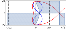
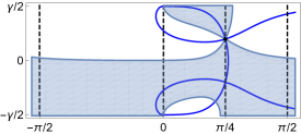
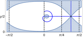
Figure 1: Behaviour of the phase $g$ in the complex plane in the asymptotic regimes R1 - R3 (left to right). The black dots denote the relevant saddle points, and the lines are lines of constant imaginary part. In the white areas ${\rm Re\,}g$ is smaller than the saddle point values, in the blue shaded area it is lager. Contours must be deformed in such a way that they pass through the relevant saddle points and do not leave the white areas.

Amazingly, it is possible to obtain the saddle-point values $g(\lambda)$, $g^{\prime\prime}(\lambda)$, $\lambda=\lambda_{1}^{\pm},\lambda_{2},\lambda_{3}$ and $[\nabla^{2}f](\lambda_{j},\lambda_{j})$, $j=2,3$ as explicit algebraic functions of $v$. This is due to the fact that (5) and (6) allow us to rewrite the saddle-point equation as

$$v\varepsilon(p)-v_{c_{1}}v_{c_{2}}\cos(p)\sin(p)=0\,.$$ (18)

This can be solved for $z=\cos^{2}(p)$ at the saddle points. Introducing the rescaled velocity parameter $r=v/{\sqrt{v_{c_{1}}v_{c_{2}}}}$ we obtain two solutions

$$2z_{\pm}=1+r^{2}\pm\begin{cases}\sqrt{(r_{1}^{2}-r^{2})(r_{2}^{2}-r^{2})}&\text{in R1, R3,}\\[8.61108pt] {\rm i}\sqrt{(r^{2}-r_{1}^{2})(r_{2}^{2}-r^{2})}&\text{in R2.}\end{cases}$$ (19)

Here $r_{1}^{2}=v_{c_{1}}/v_{c_{2}}$ and $r_{2}^{2}=v_{c_{2}}/v_{c_{1}}$. Hence, $0<r<r_{1}$ in R1, $r_{1}<r<r_{2}$ in R2 and $r_{2}<r$ in R3. From (19) we obtain $\cos(p)$ and $\sin(p)$ and therefore ${\rm e}^{{\rm i}p}$ at the saddle points. Then $\varepsilon(p)$ follows from (18).

This leads us to

$${\rm e}^{tg(\lambda_{1}^{\pm})}=(-1)^{m}\exp\bigl{\{}-{\rm i}m\bigl{(}\operatorname{arctg}\sqrt{1/z_{\pm}-1}-r^{-2}\sqrt{z_{\pm}(1-z_{\pm})}\bigr{)}\bigr{\}}$$ (20)

in R1. In R2 we find

$${\rm e}^{2tg(\lambda_{2})} =\bigl{(}r/k\bigr{)}^{m}\bigl{(}{\rm e}^{{\rm i}\varphi_{0}/2}-{\rm i}\sqrt{k^{\prime}}{\rm e}^{-{\rm i}\varphi_{1}/2}\bigr{)}^{2m}\exp\biggl{\{}\frac{2{\rm i}m\sqrt{k^{\prime}}}{rk}{\rm e}^{{\rm i}(\varphi_{0}-\varphi_{1})/2}\biggr{\}}\,,$$ (21)

$$\varphi_{s} =\operatorname{arcctg}\biggl{(}\frac{1+(-1)^{s}r^{2}}{\sqrt{(r^{2}-r_{1}^{2})(r_{2}^{2}-r^{2})}}\biggr{)}\,.$$ (22)

Finally, in R3,

$${\rm e}^{2tg(\lambda_{3})}=\exp\Bigl{\{}2m\bigl{(}\ln(\sqrt{z_{-}}-\sqrt{z_{-}-1})+r^{-2}\sqrt{z_{-}(z_{-}-1)}\bigr{)}\Bigr{\}}\,.$$ (23)

For $g^{\prime\prime}(\lambda)$ we obtain

$$\frac{\pi^{2}g^{\prime\prime}(\lambda)}{v(2kK)^{2}}=\frac{z_{+}-z_{-}}{r^{2}}\times\begin{cases}\pm{\rm i}\sqrt{z_{\pm}(1-z_{\pm})}&\text{$\lambda=\lambda_{1}^{\pm}$}\\[4.30554pt] \frac{{\rm i}r\sqrt{k^{\prime}}}{k}{\rm e}^{{\rm i}(\varphi_{0}-\varphi_{1})/2}&\text{$\lambda=\lambda_{2}$}\\[4.30554pt] -\sqrt{z_{-}(z_{-}-1)}&\text{$\lambda=\lambda_{3}$.}\end{cases}$$ (24)

It is not hard to see that the only zeros of this function as a function of $v$ are $v_{c_{1}}$ and $v_{c_{2}}$. Thus, except at these points, which mark the transition between different asymptotics regimes, the saddle points are of first order. Exactly at the transition the saddle points are of second order implying that the algebraic part decays as $t^{-4/3}$. For the saddle-point values of $[\nabla^{2}f](\lambda,\lambda)$ in R2 and R3 we obtain

$$[\nabla^{2}f](\lambda,\lambda)\\ =\frac{512(q^{2};q^{2})^{4}(q^{4};q^{4})^{2}(q^{4};q^{4},q^{4})^{8}}{(q^{2};q^{4})^{2}(q^{2};q^{4},q^{4})^{8}}\biggl{[}\frac{z(-1)^{m}(q;q^{2})^{4}}{(1-q^{-1})^{2}}+\frac{(1-z)(-q;q^{2})^{4}}{(1+q^{-1})^{2}}\biggr{]}\,,$$ (25)

where $z=z_{+}$ if $\lambda=\lambda_{2}$ in R2 and $z=z_{-}$ if $\lambda=\lambda_{3}$ in R3.

4 Discussion

Using the above explicit expressions (11), (12), (15), (17) and (20)-(25) we can easily plot our result.

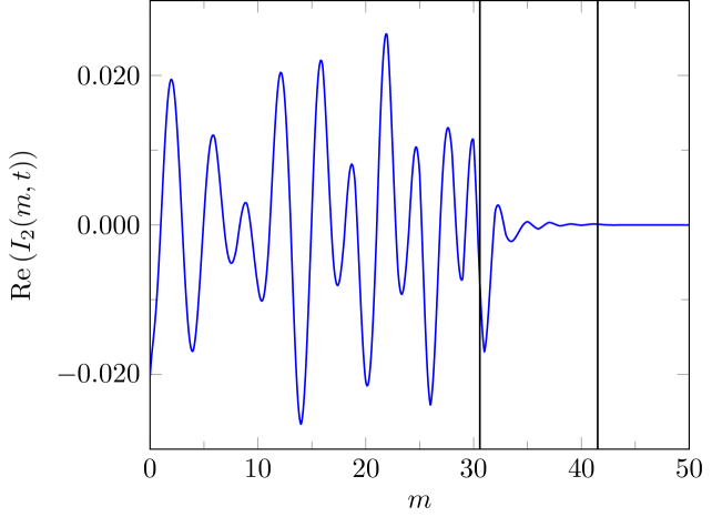
Figure 2: Real part of $I_{2}(m,t)$ as a function of $m$ for fixed $t=4$ and $\Delta=2.375$. Data points calculated for $m\in{\mathbb{Z}}$ and connected by means of splines. Vertical lines separate different asymptotic regimes, first line $m=v_{c_{1}}t$, second line $m=v_{c_{2}}t$.

Figure 2 shows the asymptotics of $I_{2}$, representing the leading dynamical contribution to the correlation function $\langle\sigma_{1}^{z}\sigma_{m+1}^{z}(t)\rangle$ (see (2)), for a fixed time $t$ as a function of the distance $m$. We see the typical features of wave propagation in a dispersive medium as they are familiar from electrodynamics [35, 8]. The wave excited locally at $m=1$ and $t=0$ contains all frequency components and hence spreads out with the maximal possible group velocity $v_{c_{1}}$. In fact it is easy to see from (6) that

$$\max_{p\in[-\pi/2,\pi/2]}|\varepsilon^{\prime}(p)|=v_{c_{1}}$$ (26)

(which is also equal to the band width $\varepsilon(0)-\varepsilon(\pi/2)$). In non-relativistic spin systems with local interactions such a maximal group velocity always exists due to the existence of a Lieb-Robinson bound [28, 11]. As in signal processing in dispersive media the wave front at $v_{c_{1}}t$ is preceded by a precursor [35, 8] extending from $m=v_{c_{1}}t$ to $m=v_{c_{2}}t$ and decaying in forward direction. In terms of ‘band parameters’ $v_{c_{2}}$ can be interpreted as twice the band centre $v_{c_{2}}=-(\varepsilon(0)+\varepsilon(\pi/2))$. The irregular appearance of the wave train in Figure 2 is due to the interference of commensurate and incommensurate components. In fact, if we split $I_{2}$ as $I_{2}(m,t)=I_{2}^{(0)}(m,t)(-1)^{m}+I_{2}^{(1)}(m,t)$, the two contributions $I_{2}^{(0)}$ and $I_{2}^{(1)}$ look more regular (see Figure 3). Figure 4 shows the same wave train as observed at a fixed site as a function of time.

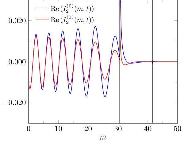
Figure 3: Real part of the two incommensurate contributions to $I_{2}(m,t)$ as a function of $m$ for fixed $t=4$ and $\Delta=2.375$ ($I_{2}^{(0)}$ blue, $I_{2}^{(1)}$ red). Vertical lines separate different asymptotic regimes, first line $m=v_{c_{1}}t$, second line $m=v_{c_{2}}t$.

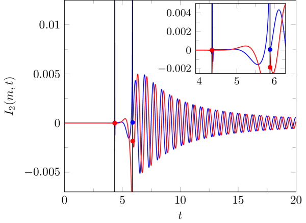
Figure 4: $I_{2}(m,t)$ as a function of $t$ for fixed $m=45$ and $\Delta=2.375$ (real part blue, imaginary part red). Vertical lines separate different asymptotic regimes, first line $t=m/v_{c_{2}}$, second line $t=m/v_{c_{1}}$. Dots denote asymptotics values exactly at the boundaries between the different regimes. From the inset one can imagine the true behaviour of the integral in the vicinity of the boundaries.

The appearance of the two different time-like and space-like regimes R1 and R3 is a consequence of the existence of the Lieb-Robinson bound. But the existence of the precursor regime R2 is not in accordance with common intuition which expects a simpler light-cone picture as in relativistic quantum field theories. This may be one of the reasons why the sine-Gordon model has often been used as an effective model for the XXZ chain in the massive antiferromagnetic regime.

Our analysis allows us two interesting conclusions. First: since the analytic behaviour of the correlation functions changes across the Stokes lines $v=v_{c_{1}}$ and $v=v_{c_{2}}$ the naive analytic continuation of an effective field theory, describing the static correlations at large distances, to the time axis would predict the wrong large-time asymptotics. Three separate theories for regimes R1, R2, R3 may be needed. Second: a general theory predicting the behaviour of auto-correlation functions is the theory of spin diffusion (see e.g. [13]). It predicts a decay of correlation functions $\sim 1/\sqrt{t}$. Hence, naively the $1/t$ behaviour of the Heisenberg-Ising chain would be called non-diffusive. However, in our saddle-point integration we have obtained a factor of $1/\sqrt{t}$ per integral which may be interpreted as a factor of $1/\sqrt{t}$ per spinon, or diffusion of spinons. The $1/t$ behaviour would then be attributed to the fact that spinons can only be created in pairs.

To avoid misunderstandings we wish to point out that there is no obvious relation of our result for the exact asymptotics of the two-point function to the result of [7], where the two-spinon contribution to the dynamical structure factor (the Fourier transform of the dynamical two-point function) was calculated. First of all [7] deals with the transversal case, while we are treating the longitudinal case. Second, to our knowledge there is no simple way to obtain the long-time, large-distance asymptotics in real space-time by Fourier techniques.

5 Summary

We have obtained asymptotically exact and explicit results for the long-time large-distance asymptotics of the longitudinal dynamical two-point functions of the Heisenberg-Ising chain in the easy-axis regime. Instead of a summary let us list the main features that might be observable in experiments:

1. Two critical velocities $v_{c_{1}}$ and $v_{c_{2}}$ and a precursor.

2. A superposition of commensurate and incommensurate components.

3. A $1/t$ decay and an oscillation with frequency $v_{c_{2}}$ in the auto-correlation function.

Acknowledgment. The authors acknowledge helpful discussions with K. Fabricius, M. Karbach, A. Klümper, R. Konik, J. Sirker and R. Weston. MD and FG acknowledge financial support by the Volkswagen Foundation and by the DFG under grant number Go 825/7-1. KKK is supported by the CNRS. His work has been partly financed by a Burgundy region PARI 2013-2014 FABER grant ‘Structures et asymptotiques d’intégrales multiples’. KKK also enjoys support from the ANR ‘DIADEMS’ SIMI 1 2010-BLAN-0120-02. JS is supported by a JSPS Grant-in-Aid for Scientific Research (C) No. 15K05208.

References

- [1] O. Babelon, H. J. de Vega, and C. M. Viallet, Analysis of the Bethe Ansatz equations of the XXZ model, Nucl. Phys. B 220 (1983), 13.
- [2] W. Bakr, J. I. Gillen, A. Peng, S. Fölling, and M. Greiner, A quantum gas microscope for detecting single atoms in a Hubbard-regime optical lattice, Nature 462 (2009), 74.
- [3] H. Bethe, Zur Theorie der Metalle. I. Eigenwerte und Eigenfunktionen der linearen Atomkette, Z. Phys. 71 (1931), 205.
- [4] D. Biegel, M. Karbach, and G. Müller, Transition rates via Bethe ansatz for the spin-1/2 planar antiferromagnet, J. Phys. A 36 (2003), 5361.
- [5] H. Boos and F. Göhmann, On the physical part of the factorized correlation functions of the XXZ chain, J. Phys. A 42 (2009), 315001.
- [6] H. Boos, M. Jimbo, T. Miwa, F. Smirnov, and Y. Takeyama, Hidden Grassmann structure in the XXZ model II: creation operators, Comm. Math. Phys. 286 (2009), 875.
- [7] A. H. Bougourzi, M. Karbach, and G. Müller, Exact two-spinon dynamic structure factor of the one-dimensional Heisenberg-Ising antiferromagnet, Phys. Rev. B 57 (1998), 11429.
- [8] L. Brillouin, Über die Fortpflanzung des Lichtes in dispergierenden Medien, Ann. Phys. 44 (1914), 203.
- [9] J.-S. Caux, H. Konno, M. Sorrell, and R. Weston, Exact form-factor results for the longitudinal structure factor of the massless XXZ model in zero field, J. Stat. Mech.: Theor. Exp. (2012), P01007.
- [10] J.-S. Caux and J. M. Maillet, Computation of dynamical correlation functions of Heisenberg chains in a field, Phys. Rev. Lett. 95 (2005), 077201.
- [11] M. Cheneau, P. Barmettler, D. Poletti, M. Endres, P. Schauß, T. Fukuhara, C. Gross, I. Bloch, C. Kollath, and S. Kuhr, Light-cone-like spreading of correlations in a quantum many-body system, Nature 481 (2012), 484.
- [12] M. Dugave, F. Göhmann, K. K. Kozlowski, and J. Suzuki, On form factor expansions for the XXZ chain in the massive regime, J. Stat. Mech.: Theor. Exp. (2015), P05037.
- [13] K. Fabricius and B. M. McCoy, Spin diffusion and the spin-1/2 XXZ chain at from exact diagonalization, Phys. Rev. B 57 (1998), 8340.
- [14] T. Fukuhara, P. Schauß, M. Endres, S. Hild, M. Cheneau, I. Bloch, and C. Gross, Microscopic observation of magnon bound states and their dynamics, Nature 502 (2013), 76.
- [15] F. Göhmann, A. Klümper, and A. Seel, Integral representation of the density matrix of the XXZ chain at finite temperature, J. Phys. A 38 (2005), 1833.
- [16] R. Hagemans and J.-S. Caux, The 4-spinon dynamical structure factor of the Heisenberg chain, J. Stat. Mech.: Theor. Exp. (2006), P12013.
- [17] S. Hild, T. Fukuhara, P. Schauß, J. Zeiher, M. Knap, E. Demler, I. Bloch, and C. Gross, Far-from-equilibrium spin transport in Heisenberg quantum magnets, Phys. Rev. Lett. 113 (2014), 147205.
- [18] M. Jimbo, K. Miki, T. Miwa, and A. Nakayashiki, Correlation functions of the XXZ model for , Phys. Lett. A 168 (1992), 256.
- [19] M. Jimbo and T. Miwa, Algebraic analysis of solvable lattice models, American Mathematical Society, 1995.
- [20] , Quantum KZ equation with and correlation functions of the XXZ model in the gapless regime, J. Phys. A 29 (1996), 2923.
- [21] M. Jimbo, T. Miwa, and F. Smirnov, Hidden Grassmann structure in the XXZ model III: introducing Matsubara direction, J. Phys. A 42 (2009), 304018.
- [22] N. Kitanine, K. K. Kozlowski, J. M. Maillet, N. A. Slavnov, and V. Terras, Algebraic Bethe ansatz approach to the asymptotic behavior of correlation functions, J. Stat. Mech.: Theor. Exp. (2009), P04003.
- [23] , A form factor approach to the asymptotic behavior of correlation functions in critical models, J. Stat. Mech.: Theor. Exp. (2011), P12010.
- [24] , The thermodynamic limit of particle-hole form factors in the massless XXZ Heisenberg chain, J. Stat. Mech.: Theor. Exp. (2011), P05028.
- [25] N. Kitanine, J. M. Maillet, and V. Terras, Form factors of the XXZ Heisenberg spin- finite chain, Nucl. Phys. B 554 (1999), 647.
- [26] , Correlation functions of the XXZ Heisenberg spin- chain in a magnetic field, Nucl. Phys. B 567 (2000), 554.
- [27] M. Lashkevich, Free field construction for the eight-vertex model: representation for form factors, Nucl. Phys. B 621 (2002), 587.
- [28] E. H. Lieb and D. W. Robinson, The finite group velocity of quantum spin systems, Comm. Math. Phys. 28 (1972), 251.
- [29] M. Mourigal, M. Enderle, A. Klöpperpieper, J.-S. Caux, A. Stunault, and H. M. Ronnow, Fractional spinon excitations in the quantum Heisenberg antiferromagnetic chain, Nat. Phys. 9 (2013), 435.
- [30] R. Orbach, Linear antiferromagnetic chain with anisotropic coupling, Phys. Rev. 112 (1958), 309.
- [31] R. G. Pereira, J. Siker, J.-S. Caux, R. Hagemann, J.-M. Maillet, S. R. White, and I. Affleck, Boson decay and the dynamical structure factor for the XXZ chain at finite magnetic field, J. Stat. Mech.: Theor. Exp. (2007), P08022.
- [32] R. G. Pereira, S. R. White, and I. Affleck, Exact edge singularities and dynamical correlations in spin-1/2 chains, Phys. Rev. Lett. 100 (2008), 027206.
- [33] J. Sato, M. Shiroishi, and M. Takahashi, Evaluation of dynamic spin structure factor for the spin-1/2 XXZ chain in a magnetic field, J. Phys. Soc. Jpn. 73 (2004), 3008.
- [34] J. F. Sherson, C. Weitenberg, M. Endres, M. Cheneau, I. Bloch, and S. Kuhr, Single-atom resolved fluorescence imaging of an atomic Mott insulator, Nature 467 (2010), 68.
- [35] A. Sommerfeld, Über die Fortpflanzung des Lichtes in dispergierenden Medien, Ann. Phys. 44 (1914), 177.
- [36] A. Virosztek and F. Woynarovich, Degenerated ground states and excited states of the anisotropic antiferromagnetic Heisenberg chain in the easy axis region, J. Phys. A 17 (1984), 3029.
- [37] E. T. Whittaker and G. N. Watson, A course of modern analysis, fourth ed., ch. 21, 22, Cambridge University Press, 1963.
- [38] F. Woynarovich, On the =0 excited states of an anisotropic Heisenberg chain, J. Phys. A 15 (1982), 2985.
- [39] C. N. Yang and C. P. Yang, One-dimensional chain of anisotropic spin-spin interactions. I. Proof of Bethe’s hypothesis for ground state in a finite system, Phys. Rev. 150 (1966), 321.
- [40] , One-dimensional chain of anisotropic spin-spin interactions. II. Properties of the ground-state energy per lattice site for an infinite system, Phys. Rev. 150 (1966), 327.
- [41] , One-dimensional chain of anisotropic spin-spin interactions. III. Applications, Phys. Rev. 151 (1966), 258.