Reinforcement Learning for
the Unit Commitment Problem

Abstract

In this work we solve the day-ahead unit commitment (UC) problem, by formulating it as a Markov decision process (MDP) and finding a low-cost policy for generation scheduling. We present two reinforcement learning algorithms, and devise a third one. We compare our results to previous work that uses simulated annealing (SA), and show a 27% improvement in operation costs, with running time of 2.5 minutes (compared to 2.5 hours of existing state-of-the-art).

I Introduction

Unit commitment (UC) is the process of determining the most cost-effective combination of generating units and their generation levels within a power system to meet forecasted load and reserve requirements, while adhering to generator and transmission constraints [2]. This is a non-linear, mixed-integer combinatorial optimization problem [3]. Low-cost solutions to this problem will directly translate into low production costs for power utilities. As the size of the problem increases, it becomes a very complex, hard to solve problem [4].
Multiple optimization approaches have been applied over the past years, such as the priority ordering methods [9, 10], dynamic programming [11], Lagrangian relaxation [13], the branch-and-bound method [15], and the integer and mixed-integer programming [16, 17]. Other, more recent methods are from the field of artificial intelligence, such as the expert systems [18], neural networks [19], fuzzy logic [20], genetic algorithms [21], and simulated annealing [1].
Many of these approaches are either purely heuristic (e.g. priority ordering) or semi-heuristic (e.g. simulated annealing) , thus are often very sensitive to choice of architecture, manual parameter tuning, and different cost functions. On the other hand, analytical methods can also introduce critical shortcomings. The branch-and-bound algorithm, for instance, suffers from an exponential growth in execution time with the size of the UC problem [15, 14]. In addition, using approximations for making it tractable for large scale systems causes solutions to be highly sub-optimal.
Therefore in our work, we take an analytical approach to the problem, while assuring it will not become intractable nor highly suboptimal in large scale systems. We use a Markov Decision Process (MDP) framework. MDPs are used to describe numerous phenomena in many fields of science [7]. Such a model is aimed to describe a decision making process, where outcomes of the process are partly random and partly under the control of the decision maker.
In this work we assume that generation cost functions of the different generators are known to the decision maker. We note that this is often not the case with European system operators, since in a European competitive electricity market, cost information is not available. However, in many other cases this information is indeed available, such as in some north American TSOs, and generation companies with multiple generation units (such a company would not know the characteristics of the power system, nevertheless it is not problematic since they do not play a role in our formulation). In addition, the UC problem can easily be extended to generate production schedules in a competitive market environment[5]. Another paper shows the framework in which a traditional cost-based unit commitment tool can be used to assist bidding strategy decisions to a day-ahead electricity pool market [6]. In general, European TSOs can approximate generation costs based on historical data (that include past and present bids they receive from generators) and market simulation. Also, in future work, the uncertainty in these approximations can be naturally expressed in our MDP model.
The rest of the paper is organized as follows. Section ii@ formulates the unit commitment problem. We then present our MDP model for the UC problem in section iii@ , and give an introduction to reinforcement learning in section iv@. The algorithms we use are presented in section v@. Then, in section vi@ we show numerical tests of our methods. Lastly, in section vii@ we summarize our work.

II Unit Commitment Problem Formulation

The problem is formulated as the following constrained optimization program.

II-A Objective

The objective is to find a feasible plan with minimal cost for operating generators to meet client demands –

$$\min_{\alpha_{i}(t),P_{i}(t),\forall i,t}\sum_{t=1}^{T}\sum_{i=1}^{N}[\alpha_{i}(t)C_{i}(P_{i}(t)) +$$ (1)

$$\alpha_{i}(t)[1-\alpha_{i}(t-1)]SC_{i}(t_{off_{i}})].$$

Where:
$a_{i}(t)=1$ when unit $i$ is turned on at time $t_{i}$, and $\alpha_{i}(t)=0$ otherwise.
$P_{i}(t)$ is the injected power $[MW]$ in unit $i$ at time $t$.
$C_{i}(P)$ is the cost $[\$]$ of injecting power $P$ in unit $i$ .
$SC_{i}(t_{off_{i}})$ is the start-up cost $[\$]$ of unit $i$ after it has been off for a time period of $t_{off_{i}}$.

II-B Constraints

Any feasible solution is subject to the following constraints:

• Load balance –

  $$\forall t:\sum_{i=1}^{N}(\alpha_{i}(t)P_{i}(t))=D(t).$$ (2)

• Generation limits –

  $$\forall i,t:\alpha_{i}(t)P_{min_{i}}\leq P_{i}(t)\leq\alpha_{i}(t)P_{max_{i}}.$$ (3)

• Set generation limits –

  $$\forall t:(\sum_{i=1}^{N}\alpha_{i}(t)P_{min_{i}}) \leq D(t),$$ (4)

  $$(\sum_{i=1}^{N}\alpha_{i}(t)P_{max_{i}}) \geq D(t)+R(t).$$

• Minimum up/down time –

  $$\forall i:t_{off_{i}} \geq t_{down_{i}},$$ (5)

  $$t_{on_{i}} \geq t_{up_{i}}.$$

Where:
$D(t)$ is the demand at time $t$.
$R(t)$ is the needed power reserve at time $t$.
$P_{min_{i}},P_{max_{i}}$ are the minimal and maximal power injections in unit $i$.
$t_{off_{i}},t_{on_{i}}$ are the minimal time periods before turning unit $i$ on/off.

II-C Costs

• Generation Cost – quadratic function of the power generated by that unit:

  $$C_{i}(P_{i})=a_{i}P_{i}^{2}+b_{i}P_{i}+c_{i}.$$ (6)

• Start-up cost – an exponentially dependent function of the number of hours a unit has been down:

  $$SC_{i}(t_{off_{i}})=e_{i}\exp(-g_{i}t_{off_{i}})+f_{i}\exp(-h_{i}t_{off_{i}}).$$ (7)

A graphical example of generation (A) and start-up (B) costs of a specific generator (with the parameters used in the experiments section) is displayed in Figure 1.

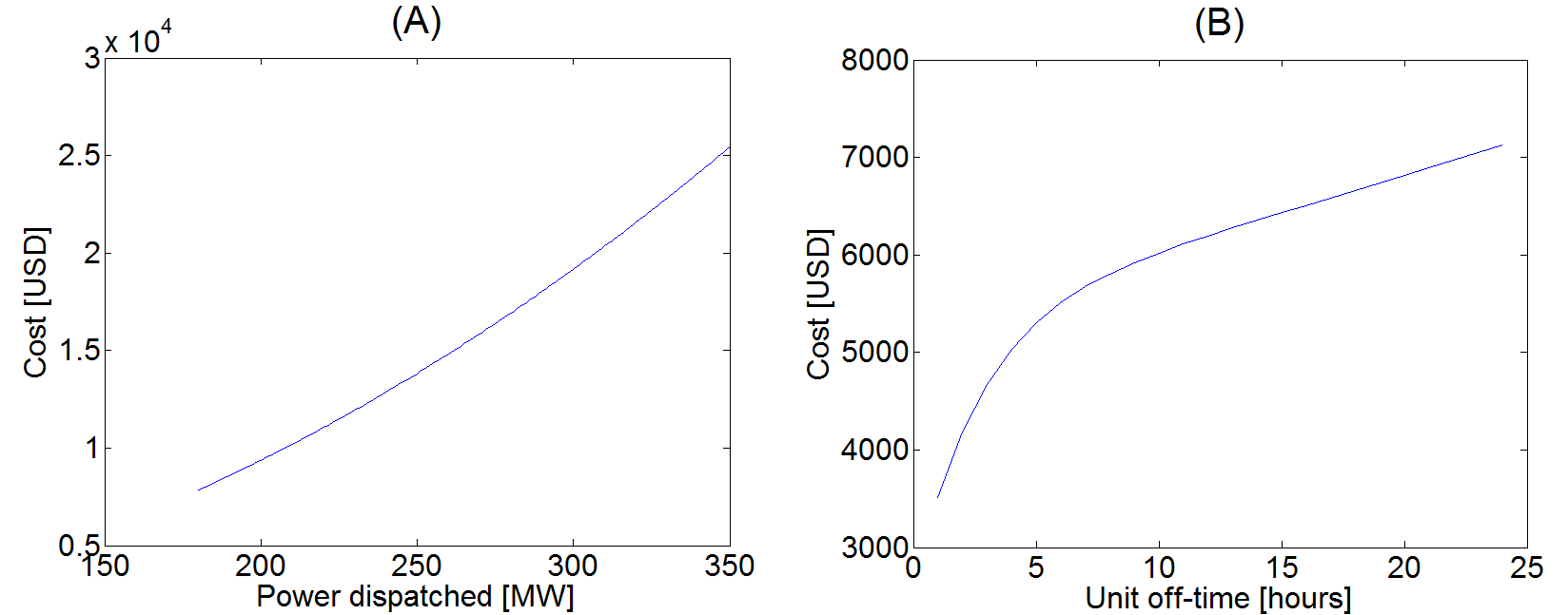
Figure 1: (A) shows the generation cost of a specific generator, and (B) shows the start-up cost of that generator, as a function of the time it was off

III Markov Decision Process Approach

Finding a global optimum is intractable for this non convex, mixed integer-quadratic problem. Therefore, unlike in [1], where a direct search in the solution space was performed, we suggest an alternative approach: decomposing the objective into a sequential decision making process. We use a Markov Decision Process 4-tuple $(S,A,P,R)$ [7] to model the system’s dynamics. Briefly, in this model at each time step, the process is in some state $s$, an action $a$ is taken, the system transitions to a next state $s^{\prime}$ according to a transition kernel $P(s,a,s^{\prime})$, and a reward $R(s,a,s^{\prime})$ is granted. Thus, the next state $s^{\prime}$ depends only on the current state $s$ and the decision maker’s action $a$.

III-A State-Space

The system’s state can be fully described by the on/off time of each of the $N$ generators, and the time of the day (negative values indicate off time):

$$S=\{-24,-23,\dots,-1,1,2,\dots,24\}^{N}\times\{1,\dots,24\}.$$

III-B Action Space

Each unit can be turned/kept on, or turned/kept off:

$$A=\{0,1\}^{N}.$$

III-C Reward

At each time step, the reward is (minus) the cost of operation of the $N$ machines:

$$R(s,a,s^{\prime})=-\sum_{i=1}^{N}[I_{[s^{\prime}_{i}>0]}C_{i}(P_{i})+I_{[s^{\prime}_{i}>0]}I_{[s_{i}<0]}SC_{i}(s_{i})].$$

The power injections $P_{i}$ are chosen by solving the appropriate constrained quadratic program (generation cost is quadratic).
By maximizing the undiscounted cumulative reward of the MDP, we minimize the original objective.

III-D Transition Kernel

Transition is deterministic: $f(s,a)=s^{\prime}$. The transition function restricts the process to satisfy the constraints of the optimization problem.
A transition example is presented in Figure 2.

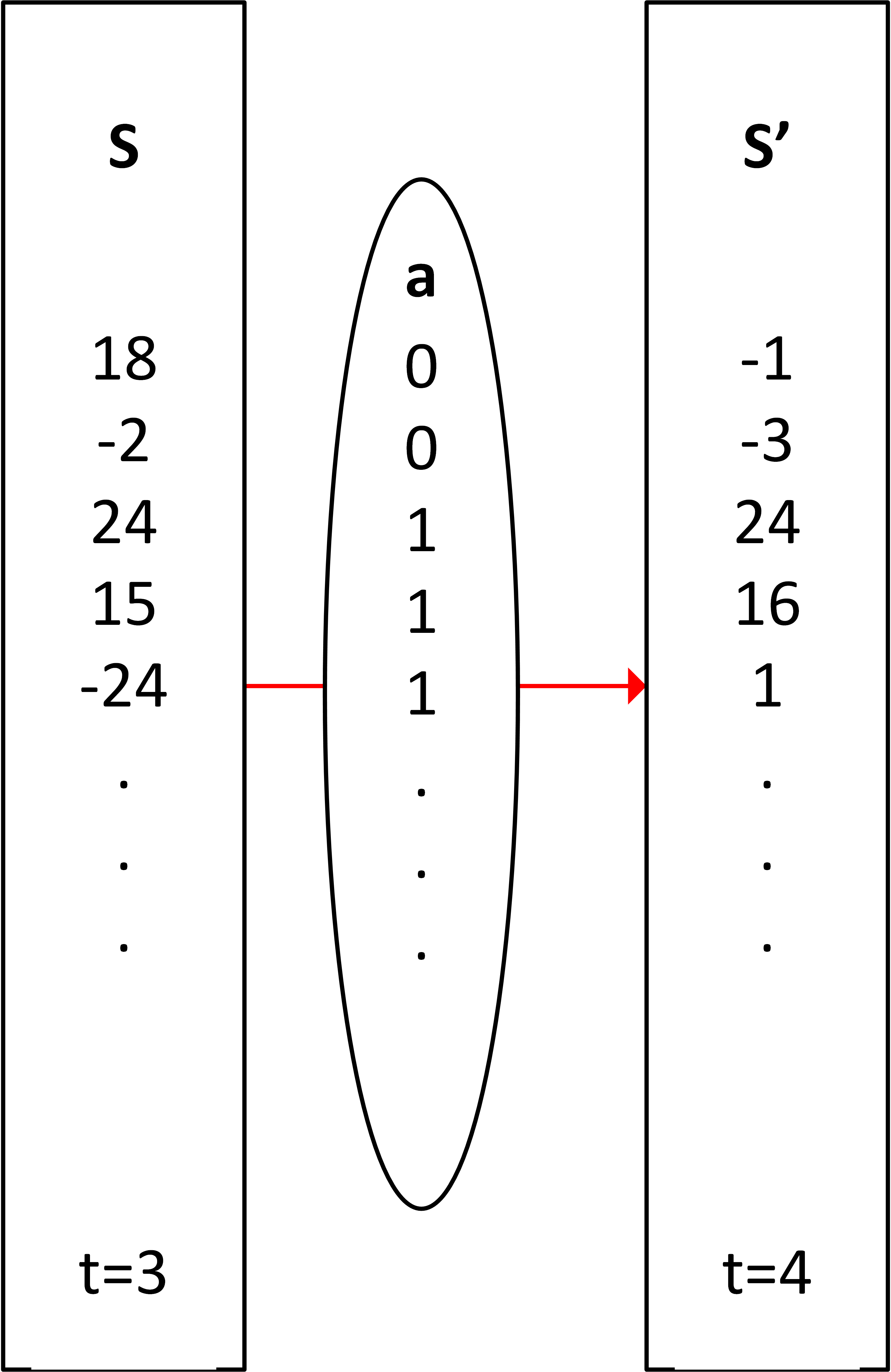
Figure 2: Example for state transition - $f(s,a)=s^{\prime}$. Generators are turned/kept on or off when an action of 1 or 0 is taken. Time is also represented in the state.

IV Reinforcement Learning

A policy is a mapping between a state-space $S$ and an action-space $A$. Given a policy, we know what action to perform at each state of the system.
For the defined MDP, our goal is the following: Find an optimal policy $\pi^{*}:S\rightarrow A$ s.t:

$$\pi^{*}=\arg\max{}_{\pi\in\Pi}\sum_{t=1}^{T}R(s_{t},\pi(s_{t}),f(s_{t},\pi(s_{t}))).$$ (8)

Where $\Pi$ is the space of all possible policies.
Reinforcement Learning (RL) [8] is a field in Machine Learning that studies algorithms that learn by interacting with the environment. The learning is done for states and actions. For each state $s$, given a policy $\pi$, a state value $v^{\pi}(s)$ is defined as:

$$v^{\pi}(s)=\sum_{t=1}^{T}R(s_{t},\pi(s_{t}),f(s_{t},\pi(s_{t})))\quad\textrm{for}\quad s_{1}=s.$$ (9)

V Reinforcement Learning Algorithmic Solutions

In this section we present three different reinforcement learning algorithms for solving 8.

V-A Algorithm 1 – Approximate Policy Iteration (API) using Classification

An extension to the state value $v^{\pi}(s)$ defined above, is the state-action value function $Q^{\pi}(s,a)$, which denotes the value of performing action $a$ (regardless of the policy $\pi$), and only after that – following policy $\pi$. In our first algorithm we use the state-action value function. This function is defined the set of all $(s,a)$ pairs, which is of size $|S|\cdot|A|$.

V-A1 Approximation

Our state-space grows exponentially with $N$: $|S|=24\cdot 48^{N}$, as well as the action-space: $|A|=2^{N}$. Already for $N\geq 4$, it is impossible to find the exact value for each state-action pair. We therefore use an approximation method for evaluating the state-action value function $Q^{\pi}(s,a)$. We use feature-based regression, which significantly lowers the dimension of $Q^{\pi}(\cdot,\cdot)$ from $|S|\cdot|A|$ to $dim(\phi(s,a))$, the dimension of the feature vector $\phi(s,a)$. We use 4 binary features for each generator $i$, for each of the possible ’interesting’ zones it can be in:

$$s_{i} <-t_{off_{i}},$$

$$-t_{off_{i}}\leq s_{i} <0,$$

$$0< s_{i} \leq t_{on_{i}},$$

$$t_{on_{i}}< s_{i}$$ .

The features are then duplicated $N$ times and zeroed out at indices where the action vector is $0$. The result is again duplicated into two – for distinguishing between $(s,a)$ pairs that will lead to a catastrophe (transition to infeasible states). We end up with a feature vector $\phi(s,a)$ of dimension that is only quadratic in $N$: $dim(\phi(s,a))=2\cdot 4\cdot N^{2}$.

V-A2 Policy Iteration Algorithm

The basic algorithm is policy iteration [8]. This well-known algorithm iterates between two stages: evaluation of the states’ values under a fixed policy, and the improvement of the policy using the learned values. We perform the evaluation using the SARSA [8] algorithm (with epsilon-greedy exploration), and the improvement is simply done using the following maximization (for step $k$):

$$\pi_{k}(s)=\operatorname*{arg\,max}_{a\in A}Q_{k}(s,a)=\operatorname*{arg\,max}_{a\in A}\phi(s,a)^{T}w_{k}.$$ (10)

V-A3 Policy Representation

The biggest challenge in enabling policy iteration for our problem is the choice of policy representation. On the one hand, the policy should be defined for all states $s\in S$. On the other hand, it can practically only be trained using a very small fraction of this huge state-space. Also, its output is a selection from the enormous space of actions.
To handle the above difficulties, we chose the policy to be a classifier, that classifies states into actions. This gives rise to a large-scale multi-class classification task ($2^{N}$ optional classes), which is considered to be a difficult problem on its own. We tackle that by using a hierarchical classifier with a tree-based structure: Each node classifies an action bit and splits into two nodes for the next bit. Classification is done in the feature-space. The perceptron algorithm [24] is used a the basic binary classifier (online updates can be made to save memory). A different tree is stored per each time-step.
Note that this is not a decision-tree classifier, but multiple binary hyper-plane based classifiers that are being traversed through in a sequential manner. The leafs determine the final action prediction (encapsulate the path).

Initialize:
$\alpha$ - SARSA step size
$\epsilon$ - exploration parameter
$N_{pi}$ - iteration count
$\pi_{0}$ - intial policy
$\phi$ - basis functions

1:  for $k=1$ to $k=N_{pi}$ do

2:     $w_{k}=SARSA(\pi_{k},\alpha,\epsilon)$

3:     for all $s\in S$ do

4:        $a^{*}=\operatorname*{arg\,max}_{a\in A}\phi(s,a)^{T}w_{k}$

5:        $\pi_{k}=updateClassifier(a^{*},\pi_{k})$

6:     end for

7:  end for

8:  return  $\pi_{N_{pi}}$

Algorithm 1 Approximate Policy Iteration using Classification

V-B Algorithm 2 – Tree Search

An MDP can be represented as a tree, where each node is a state and each edge corresponds to an action. In our problem, we can theoretically express the tree explicitly, where the edges include the exact reward of the transition since transitions and rewards are deterministic. Let us also denote $s^{t}_{j}$ so be the $j$-th state at time-step $t$.

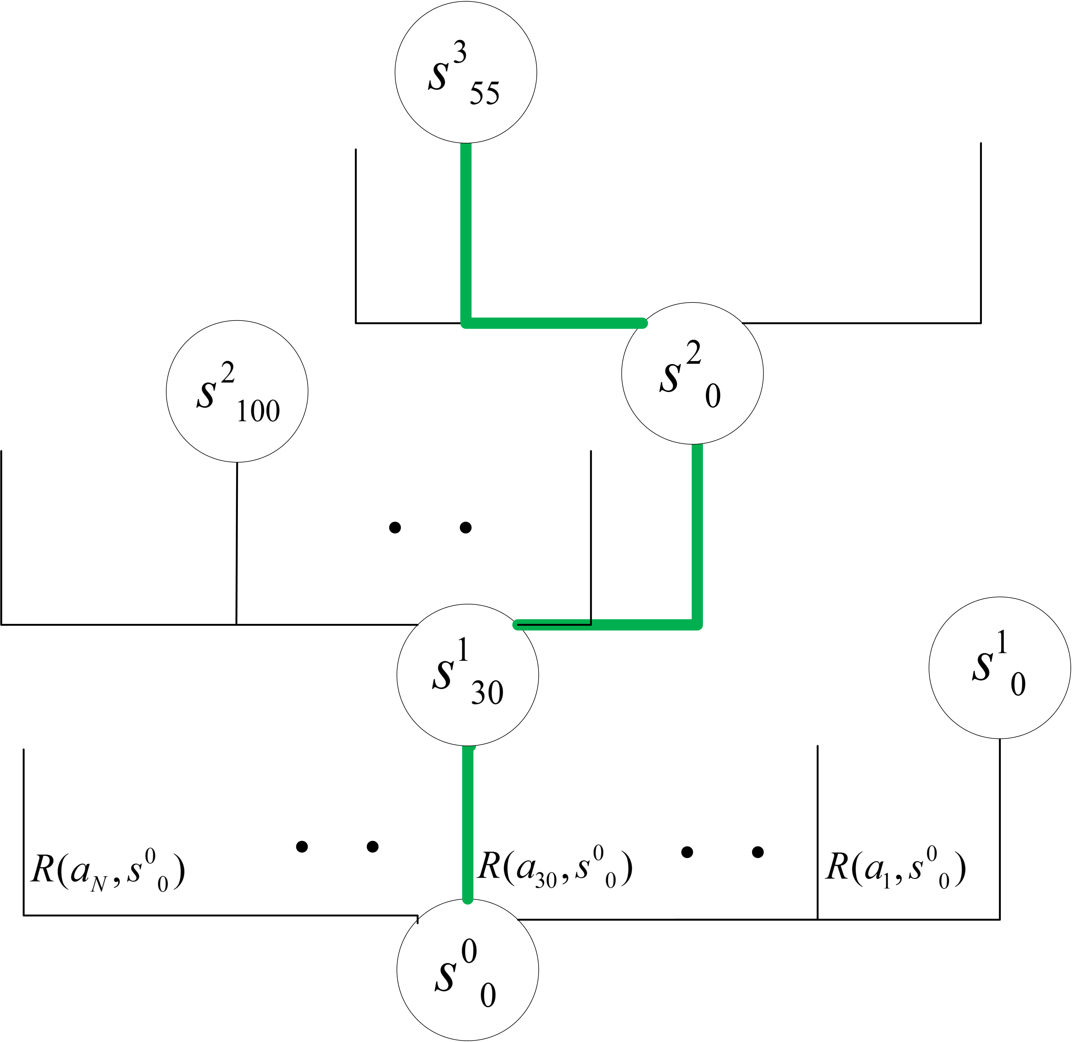
Figure 3: Visualisation of algorithm 2 – tree search. Nodes are states, edges are transitions with the corresponding rewards.

Under this representation, finding an optimal policy $\pi^{*}$ corresponds to finding the largest aggregated reward path from the root (initial state $s^{0}_{0}$).
However, since the number of possible paths in the tree is in the order of $|A|^{T}=2^{N\cdot T}$ , naively searching the tree for an optimal path is intractable for a problem of our size. Therefore in our tree search algorithm we limit the time horizon in which we search to be $H$ ($H<T$). I.e, tree search seeks a lookahead policy by iterating through all of the possible outcomes in a limited lookahead horizon $H$. Our algorithm contains the two following main components:

V-B1 Algorithm 2.1

The first part of the algorithm, $findBestAction(s^{t},H)$, recursively searches for the next best action that can be taken from state $s^{t}$, by iterating on all possible actions from that state. ”Best” in this case, is considered with regard to all possible paths in a lookahead horizon of $H$ time-steps ahead. That is, it finds $a^{t}$, the first action in the vector $\boldsymbol{a}=(a^{t},a^{t+1},\dots,a^{t+H})$, where

$$\boldsymbol{a}=\operatorname*{arg\,max}_{\boldsymbol{a^{\prime}}\in A^{H}}\sum_{t^{\prime}=t}^{t+H}R(s^{t^{\prime}},a^{t^{\prime}},f(s^{t^{\prime}},a^{t^{\prime}})).$$

1:  if $H==0\mbox{ }\textbf{or}{}\mbox{ }t==T-1$ then

2:     return  $(0,0)$

3:  end if

4:  $v_{m}=-\infty,a_{m}=\bar{0}$

5:  for all $a\in A$ do

6:     $s^{t+1}=f(s^{t},a)$

7:     $(a^{t+1},v^{t+1})=findBestAction(s^{t+1},H-1)$

8:     $v^{t}=R(s^{t},a,s^{t+1})+v^{t+1}$

9:     if $v^{t}\geq v_{m}$ then

10:        $a_{m}=a,v_{m}=v$

11:     end if

12:  end for

13:  return  $(a_{m},v_{m})$

Algorithm 2.1 $(a_{m},v_{m})=findBestAction(s^{t},H)$

V-B2 Algorithm 2.2

The second component of our tree search algorithm finds the optimal lookahead policy by initiating $findBestPolicy$ per each time step from $t=0$ to $t=T-1$.

1:  for $t=0$ to $t=T-1$ do

2:     $(a_{m},v_{m})=findBestAction(s^{t},H)$

3:     $\pi(s^{t})=a_{m}$

4:     $s^{t+1}=f(s^{t},a_{m})$

5:  end for

6:  return  $\pi$

Algorithm 2.2 $\pi=treeSearch(s^{t},H)$

V-B3 Improve by Sub-sampling

We can take advantage of a certain property of this problem: it is very unlikely that in ”good” (highly rewarding) paths, subsequent actions will differ significantly from each other. This is both because of the high start-up costs of generators, and because of the minimal up/down time limitation (rapidly switching different machines on/off can lead to infeasible states, where there aren’t enough available generators to satisfy demand).
Exploiting this property, we added an improvement for our algorithm. Instead of iterating throughout all actions when searching for the best one at time $t+1$, we only sample small deviations from last best action at time $t$ (denoted as $a^{t*}$). For the sampling we use a probability density over the action $a^{t+1}$, with an inverse relation to $\|a^{t*}-a^{t+1}\|_{2}$. This improvement significantly reduces the runtime, and can also enable setting a larger value for $H$. In the experiments section, we test the usability of our improvement and compare it to the original approach.

V-C Algorithm 3 – Back Sweep

Our ”Back Sweep” algorithm is a novel algorithm, inspired by the concept in dynamic programming of backtracking from the terminal time and going backwards. That way, we have a reliable estimation of the value of future states, and can base decisions correctly based on that knowledge of future values. The main novelty is in sampling ’interesting’ (potentially beneficial) areas of the state-space, and use a nearest neighbour (NN) approximation of them in the Bellman update step (defined below).

V-C1 Algorithm 3.1

First of two parts of the algorithm is evaluation the optimal value of each sampled state, $v^{*}(s)$. The optimal value is the value of states when using the optimal policy as defined in 8:

$$v^{*}(s)=\sup\limits_{\pi\in\Pi}v^{\pi}(s).$$ (11)

It is found using Bellman’s update step, that lies in the heart of the algorithm:

$$v^{*}(s)=\max\limits_{a\in A}[R(s,a,s^{\prime})+v^{*}(s^{\prime})].$$ (12)

1:  Initialize ${\cal D}=\emptyset,\tilde{s}=s^{T}$

2:  for $t=T-1$ to $0$ do

3:     $\underline{S}^{t}=$ $sampleEnvironment(\tilde{s},N_{s})$

4:     for $i=1$ to $N_{s}$ do

5:        $\hat{v}^{*t}(s^{t}_{i})=\max_{a\in A}[R(s^{t}_{i},a,f(s^{t}_{i},a))+\hat{v}^{*t+1}(NN(f(s^{t}_{i},a),\cal D))]$

6:     end for

7:     ${\cal{\cal D}=D}\cup\{(\underline{S}^{t},\hat{\underline{V}}^{*t})\}$

8:     $\tilde{s}=\arg\max_{s}\hat{\underline{V}}^{*t}(s)$

9:  end for

10:  return  $\cal D$

Algorithm 3.1 ${\cal D}=evaluateStates(N_{s},s_{0})$

• $sampleEnvironment(\tilde{s},N_{s})$ returns $N_{s}$ samples of states that are ’close’ to $\tilde{s}$. Closeness is quantified using a metric we defined.

• $NN(s,\cal D)$ returns the nearest-neighbor state from all states that are in the $(s,v)$ pairs in $\cal D$.

V-C2 Algorithm 3.2

The second part of the algorithm will produce a greedy policy via one quick sweep forward, beginning from the initial state $s^{0}$. This policy is greedy since at each step we choose the best possible action, and it is proven that for exact $v^{*}$ values, it will also be the optimal policy [8].

1:  for $t=0$ to $T-1$ do

2:     $a^{t}=\arg\max_{a\in A}[R(s^{t},a,f(s^{t},a))+\hat{v}^{*t+1}(NN(f(s^{t}_{i},a),\cal D))]$

3:     $\pi(s^{t})=a^{t}$

4:     $s^{t+1}=f(s^{t},a^{t})$

5:  end for

6:  return  $\pi$

Algorithm 3.2 $\pi=findGreedyPolicy({\cal D})$

VI Experiments

In order to test the performance of the three proposed algorithms, we used Matlab [22] to implement and run them on a problem setting with $N=12$ generators, a 24-hour schedule ($T=24$), with parameters taken from [1]. In [1], an Adaptive Simulated Annealing (SA) technique is used, and a minimal objective of $644,951 is achieved.

VI-A Algorithm 1

Algorithm 1 only performed well on a smaller setting of the problem ($N=8$, $T=12$) and was not included in Table I. In spite of that, we chose to present algorithm 1 in this paper as a baseline. API is a very commonly used algorithm in the reinforcement learning literature. On top of that, the policy structure we devised enabled the algorithm the leap from performing only on a $N=4$, $T=8$ setting, to the $N=8$, $T=12$ setting.
We also find value in understanding its weaknesses - it could not handle a larger scheme due to its forward-looking mechanism. Since it starts with a random policy, state evaluation is very poor at the beginning (compared to their optimal value), and the improvement becomes slow and inefficient throughout iterations. Magnification of this problem is taking place since unlike in infinite horizon formulations, different policies are used for different time-steps.

VI-B Algorithm 2

Algorithm 2 was tested with two different lookahead horizons: $H=1$ and $H=3$. The extremely low run-time for $H=1$ make it the most preferable algorithm for this problem, in spite of the small increase in objective cost.
The large difference in run times for the two cases is due to the exponential complexity in $H$.
The improved version of algorithm 2, which includes sub-sampling of actions, enables a reduction in run-time, while compromising negligible value in the overall cost.

VI-C Algorithm 3

The terminal state of algorithm 2’s solution is fed as an initial state to algorithm 3, Sampling count used was $N_{s}=50$.

VI-D Result Comparison

TABLE I: Experiment results of the different algorithms

Algorithm	Objective cost [$]	Run-time [min]
SA in [1]	702,379	N/A
Adaptive SA in [1]	644,951	145
Tree Search, H=1	512,850	2.5
Tree Search, H=3	512,217	240
Sub-sampled Tree Search, H=3	512,850	85
Back Sweep	511,500	60

Table I summarizes the experiment’s results. The solutions we obtain are very similar to each other, all around $512,000 for operation cost.
Algorithm 2 produces a 27% improvement in objective value compared to the state-of-the-art algorithm presented in [1], which achieved a minimal objective of $644,951, with only 2.5 minutes of running time, compared to 2.5 hours in [1].

VII Summary

In this paper we introduced three algorithms from the field of reinforcement learning, one of them novel. We formulated the unit commitment problem as a Markov Decision Process and solved it using the three algorithms (successfully with two).
The superior results in the experiments section lead us to believe that modelling the UC problem as an MDP is highly advantageous over other existing methods, which were mentioned in the introduction section.
An additional significant improvement is the option of an immediate extension for a stochastic environment, which include consideration of uncertainties. Demand, generation capacity, and generation costs can be easily modelled as stochastic by setting the appropriate probabilistic transition kernel and reward function in our existing MDP model. The algorithms presented in the paper need not change for obtaining a solution for such a probabilistic version. This transition to an uncertain formulation might be very challenging [25, 26], or even impossible when using other optimization methods.
We intend to test our algorithms under such uncertainty conditions, and possibly to change the formulation in order to obtain a risk-averse strategy for the unit commitment. This can be done by including a risk criterion in the objective, that will take into account contingencies, shut-downs, and load shedding costs while considering the probabilities of those events to happen.

References

- [1] Dudek, Grzegorz. ”Adaptive simulated annealing schedule to the unit commitment problem.” Electric Power Systems Research 80.4 (2010): 465-472.
- [2] Padhy, Narayana Prasad. ”Unit commitment-a bibliographical survey.” Power Systems, IEEE Transactions on 19.2 (2004): 1196-1205. APA
- [3] Sheble, Gerald B., and George N. Fahd. ”Unit commitment literature synopsis.” Power Systems, IEEE Transactions on 9.1 (1994): 128-135.
- [4] Orero, S. O., and M. R. Irving. ”Large scale unit commitment using a hybrid genetic algorithm.” International Journal of Electrical Power & Energy Systems 19.1 (1997): 45-55.
- [5] Arroyo, José M., and Antonio J. Conejo. ”Optimal response of a thermal unit to an electricity spot market.” Power Systems, IEEE Transactions on 15.3 (2000): 1098-1104.
- [6] Borghetti, A., et al. ”Using of a cost-based unit commitment algorithm to assist bidding strategy decisions.” Power Tech Conference Proceedings, 2003 IEEE Bologna. Vol. 2. IEEE, 2003.
- [7] Puterman, Martin L. Markov decision processes: discrete stochastic dynamic programming. Vol. 414. John Wiley & Sons, 2009.
- [8] Sutton, Richard S., and Andrew G. Barto. Introduction to reinforcement learning. MIT Press, 1998.
- [9] Lee, Fred N. ”Short-term thermal unit commitment-a new method.” Power Systems, IEEE Transactions on 3.2 (1988): 421-428.
- [10] Senjyu, Tomonobu, et al. ”A technique for unit commitment with energy storage system.” International Journal of Electrical Power & Energy Systems 29.1 (2007): 91-98.
- [11] Snyder, Walter L., H. David Powell, and John C. Rayburn. ”Dynamic programming approach to unit commitment.” Power Systems, IEEE Transactions on 2.2 (1987): 339-348.
- [12] Hargreaves, Jeremy J., and Benjamin F. Hobbs. ”Commitment and dispatch with uncertain wind generation by dynamic programming.” Sustainable Energy, IEEE Transactions on 3.4 (2012): 724-734.
- [13] Virmani, Sudhir, et al. ”Implementation of a Lagrangian relaxation based unit commitment problem.” Power Systems, IEEE Transactions on 4.4 (1989): 1373-1380.
- [14] Cheng, Chuan-Ping, Chih-Wen Liu, and Chun-Chang Liu. ”Unit commitment by Lagrangian relaxation and genetic algorithms.” Power Systems, IEEE Transactions on 15.2 (2000): 707-714.
- [15] Cohen, Arthur I., and Miki Yoshimura. ”A branch-and-bound algorithm for unit commitment.” Power Apparatus and Systems, IEEE Transactions on 2 (1983): 444-451.
- [16] Carrión, Miguel, and José M. Arroyo. ”A computationally efficient mixed-integer linear formulation for the thermal unit commitment problem.” Power Systems, IEEE Transactions on 21.3 (2006): 1371-1378.
- [17] Ostrowski, James, Miguel F. Anjos, and Anthony Vannelli. ”Tight mixed integer linear programming formulations for the unit commitment problem.” Power Systems, IEEE Transactions on 27.1 (2012): 39-46.
- [18] Ouyang, Z., and S. M. Shahidehpour. ”Short-term unit commitment expert system.” Electric power systems research 20.1 (1990): 1-13.
- [19] Kumar, S. Senthil, and V. Palanisamy. ”A dynamic programming based fast computation Hopfield neural network for unit commitment and economic dispatch.” Electric power systems research 77.8 (2007): 917-925.
- [20] Saber, Ahmed Yousuf, et al. ”Fuzzy unit commitment solution—a novel twofold simulated annealing approach.” Electric Power Systems Research 77.12 (2007): 1699-1712.
- [21] Dudek, Grzegorz. ”Unit commitment by genetic algorithm with specialized search operators.” Electric Power Systems Research 72.3 (2004): 299-308.
- [22] www.matlab.com
- [23] Bertsekas, Dimitri P., and John N. Tsitsiklis. ”Neuro-dynamic programming: an overview.” Decision and Control, 1995., Proceedings of the 34th IEEE Conference on. Vol. 1. IEEE, 1995.
- [24] Freund, Yoav, and Robert E. Schapire. ”Large margin classification using the perceptron algorithm.” Machine learning 37.3 (1999): 277-296.
- [25] Jiang, Ruiwei, Jianhui Wang, and Yongpei Guan. ”Robust unit commitment with wind power and pumped storage hydro.” Power Systems, IEEE Transactions on 27.2 (2012): 800-810.
- [26] Aminifar, Farrokh, Mahmud Fotuhi-Firuzabad, and Mohammad Shahidehpour. ”Unit commitment with probabilistic spinning reserve and interruptible load considerations.” Power Systems, IEEE Transactions on 24.1 (2009): 388-397.