The Population Posterior
and Bayesian Inference on Streams

Abstract

Many modern data analysis problems involve inferences from streaming data. However, streaming data is not easily amenable to the standard probabilistic modeling approaches, which assume that we condition on finite data. We develop population variational Bayes, a new approach for using Bayesian modeling to analyze streams of data. It approximates a new type of distribution, the population posterior, which combines the notion of a population distribution of the data with Bayesian inference in a probabilistic model. We study our method with latent Dirichlet allocation and Dirichlet process mixtures on several large-scale data sets.

1 Introduction

Probabilistic modeling has emerged as a powerful tool for data analysis. It is an intuitive language for describing assumptions about data and provides efficient algorithms for analyzing real data under those assumptions. The main idea comes from Bayesian statistics. We encode our assumptions about the data in a structured probability model of hidden and observed variables; we condition on a data set to reveal the posterior distribution of the hidden variables; and we use the resulting posterior as needed, for example to form predictions through the posterior predictive distribution or to explore the data through the posterior expectations of the hidden variables.

Many modern data analysis problems involve inferences from streaming data. Examples include exploring the content of massive social media streams (e.g., Twitter, Facebook), analyzing live video streams, modeling the preferences of users on an online platform for recommending new items, and predicting human mobility patterns for anticipatory computing. Such problems, however, cannot easily take advantage of the standard approach to probabilistic modeling, which always assumes that we condition on a finite data set. This might be surprising to some readers; after all, one of the tenets of the Bayesian paradigm is that we can update our posterior when given new information. (“Yesterday’s posterior is today’s prior.”). But there are two problems with using Bayesian updating on data streams.

The first problem is that Bayesian posteriors will become overconfident. Conditional on never-ending data, most posterior distributions (with a few exceptions) result in a point mass at a single configuration of the latent variables. That is, the posterior contains no variance around its idea of the hidden variables that generated the observed data. In theory this is sensible, but only in the impossible scenario where the data truly came from the proposed model. In practice, all models provide approximations to the data-generating distribution, and we always harbor uncertainty about the model (and thus the hidden variables) even in the face of an infinite data stream.

The second problem is that the data stream might change over time. This is an issue because, frequently, our goal in applying probabilistic models to streams is not to characterize how they change, but rather to accommodate it. That is, we would like for our current estimate of the latent variables to be accurate to the current state of the stream and to adapt to how the stream might slowly change. (This is in contrast, for example, to time series modeling.) Traditional Bayesian updating cannot handle this. Either we explicitly model the time series, and pay a heavy inferential cost, or we tacitly assume that the data are independent and exchangeable.

In this paper we develop new ideas for analyzing data streams with probabilistic models. Our approach combines the frequentist notion of the population distribution with probabilistic models and Bayesian inference.

Main idea: The population posterior. Consider a latent variable model of $\alpha$ data points. (This is unconventional notation; we will describe why we use it below.) Following [hoffman_stochastic_2013], we define the model to have two kinds of hidden variables: global hidden variables $\beta$ contain latent structure that potentially governs any data point; local hidden variables $z_{i}$ contain latent structure that only governs the $i$th data point. Such models are defined by the joint,

$$p(\beta,\mathbf{z},\mathbf{x})=p(\beta)\prod_{i=1}^{\alpha}p(x_{i},z_{i}\>|\>\beta),$$ (1)

where $\mathbf{x}=x_{1:\alpha}$ and $\mathbf{z}=z_{1:\alpha}$. Traditional Bayesian statistics conditions on a fixed data set $\mathbf{x}$ to obtain the posterior distribution of the hidden variables $p(\beta,\mathbf{z}\>|\>\mathbf{x})$. As we discussed, this framework cannot accommodate data streams. We need a different way to use the model.

We define a new distribution, the population posterior, which enables us to consider Bayesian modeling of streams. Suppose we observe $\alpha$ data points independently from the underlying population distribution, $\mathbf{X}\sim F_{\alpha}$. This induces a posterior $p(\beta,\mathbf{z}\>|\>\mathbf{X})$, which is a function of the random data. The expected value of this posterior distribution is the population posterior,

$$\mathbb{E}_{F_{\alpha}}\left[p(\mathbf{z},\beta|\mathbf{X})\right]=\mathbb{E}_{F_{\alpha}}\left[\frac{p(\beta,\mathbf{z},\mathbf{X})}{p(\mathbf{X})}\right].$$ (2)

Notice that this distribution is not a function of observed data; it is a function of the population distribution $F$ and the data set size $\alpha$. The data set size is a parameter that can be set. This parameter controls the variance of the population posterior, and so depends on how close the model is to the true data distribution.

We have defined a new problem. Given an endless stream of data points coming from $F$ and a value for $\alpha$, our goal is to approximate the corresponding population posterior. We will use variational inference and stochastic optimization to approximate the population posterior. As we will show, our algorithm justifies applying a variant of stochastic variational inference [hoffman_stochastic_2013] to a data stream. We used this technique to analyze several data streams with modern probabilistic models, such as latent Dirichlet allocation and Dirichlet process mixtures. With held out likelihood as a measure of model fitness, we found our method to give better models of the data than approaches based on full Bayesian inference [hoffman_stochastic_2013] or Bayesian updating [broderick_streaming_2013].

Related work. Several methods exist for performing inference on streams of data. Refs. [yao_efficient_2009, ahmed_online_2011, doucet_sequential_2000] propose extending Markov chain Monte Carlo methods for streaming data. However, sampling-based approaches do not scale to massive datasets. The variational approximation enables more scalable inference. Ref. [honkela_online_2003] propose online variational inference by exponentially forgetting the variational parameters associated with old data. Ref. [hoffman_stochastic_2013] also decay parameters derived from old data, but interpret this action in the context of stochastic optimization, bringing guarantees of convergence to a local optimum. This gradient-based approach has enabled the application of more advanced probabilistic models to large-scale data sets. However, none of these methods are applicable to streaming data, because they implicitly rely on the data being of known size (even when based on subsampling data points to obtain noisy gradients).

To apply the variational approximation to streaming data, Ref. [broderick_streaming_2013] and Ref. [ghahramani_online_2000] both propose performing Bayesian updating to the approximating family. Their method uses the latest approximation having seen $n$ data points as a prior to be updated using the approximation of the next data point (or mini-batch) using Bayes’ rule. Ref. [tank_streaming_2015] adapt this framework to nonparametric mixture modelling. Here we take a different approach, by changing the overall variational objective to incorporate a population distribution $F$ and following stochastic gradients of this new objective.

Independently, Ref. [theis_trust_2015] apply SVI to streaming settings by accumulating new data points into a growing window, then uniformly sampling from this window to update the variational parameters. Our method justifies that approach. Further, they propose updating parameters along a trust region, instead of following (natural) gradients, as a way of mitigating local optima. This innovation can be incorporated into our method.

2 Variational Inference for the Population Posterior

We develop population variational Bayes, a method for approximating the population posterior in Eq. 2. Our method is based on variational inference and stochastic optimization.

The F-ELBO. The idea behind variational inference is to approximate difficult-to-compute distributions through optimization [jordan_introduction_1999, wainwright_graphical_2008]. We introduce an approximating family of distributions over the latent variables $q(\beta,\mathbf{z})$ and try to find the member of $q(\cdot)$ that minimizes the Kullback-Leibler (KL) divergence to the target distribution.

Population variational Bayes (VB) uses variational inference to approximate the population posterior in Eq. 2. It aims to solve the following problem,

$$q^{*}(\beta,\mathbf{z})=\min_{q}\mathrm{KL}(q(\beta,\mathbf{z})||\mathbb{E}_{F_{\alpha}}[p(\beta,\mathbf{z}\>|\>\mathbf{X})]).$$ (3)

As for the population posterior, this objective is a function of the population distribution of $\alpha$ data points $F_{\alpha}$. Notice the difference to classical VB. In classical VB, we optimize the KL divergence between $q(\cdot)$ and a posterior, $\mathrm{KL}(q(\beta,\mathbf{z})||p(\beta,\mathbf{z}\>|\>\mathbf{x}))$. Its objective is a function of a fixed data set $\mathbf{x}$; the objective in Eq. 3 is a function of the population distribution $F_{\alpha}$.

We will use the mean-field variational family, where each latent variable is independent and governed by a free parameter,

$$q(\beta,\mathbf{z})=q(\beta\>|\>\lambda)\prod_{i=1}^{\alpha}q(z_{i}\>|\>\phi_{i}).$$ (4)

The free variational parameters are the global parameters $\lambda$ and local parameters $\phi_{i}$. Though we focus on the mean-field family, extensions could consider structured families [saul_exploiting_1996, hoffman_structured_2015], where there is dependence between variables.

In classical VB, where we approximate the usual posterior, we cannot compute the KL. Thus, we optimize a proxy objective called the ELBO (evidence lower bound) that is equal to the negative KL up to an additive constant. Maximizing the ELBO is equivalent to minimizing the KL divergence to the posterior.

In population VB we also optimize a proxy objective, the F-ELBO. The F-ELBO is an expectation of the ELBO under the population distribution of the data,

$$\mathcal{L}(\lambda,\phi;F_{\alpha})=\mathbb{E}_{F_{\alpha}}\left[\mathbb{E}_{q}\left[\log p(\beta)-\log q(\beta\>|\>\lambda)+\sum_{i=1}^{\alpha}\log p(X_{i},Z_{i}\>|\>\beta)-\log q(Z_{i})]\right]\right].$$ (5)

The F-ELBO is a lower bound on the population evidence $\log\mathbb{E}_{F_{\alpha}}[p(\mathbf{X})]$ and a lower bound on the negative KL to the population posterior. (See Appendix A.) The inner expectation is over the latent variables $\beta$ and $\mathbf{Z}$, and is a function of the variational distribution $q(\cdot)$. The outer expectation is over the $\alpha$ random data points $\mathbf{X}$, and is a function of the population distribution $F_{\alpha}(\cdot)$. The F-ELBO is thus a function of both the variational distribution and the population distribution.

As we mentioned, classical VB maximizes the (classical) ELBO, which is equivalent to minimizing the KL. The F-ELBO, in contrast, is only a bound on the negative KL to the population posterior. Thus maximizing the F-ELBO is suggestive but is not guaranteed to minimize the KL. That said, our studies show that this is a good quantity to optimize and in Appendix A we show that the F-ELBO does minimize $\mathbb{E}_{F_{\alpha}}[\mathrm{KL}(q(\mathbf{z},\beta)||p(\mathbf{z},\beta|\mathbf{X}))]$. As we will see, the ability to sample from $F_{\alpha}$ is the only additional requirement for maximizing the F-ELBO, using stochastic gradients.

Conditionally conjugate models. In the next section we will develop a stochastic optimization algorithm to maximize Eq. 5. First, we describe the class of models that we will work with.

Following [hoffman_stochastic_2013] we focus on conditionally conjugate models. A conditionally conjugate model is one where each complete conditional—the conditional distribution of a latent variable given all the other latent variables and the observations—is in the exponential family. This class includes many models in modern machine learning, such as mixture models, topic models, many Bayesian nonparametric models, and some hierarchical regression models. Using conditionally conjugate models simplifies many calculations in variational inference.

Under the joint in Eq. 1, we can write a conditionally conjugate model with two exponential families:

$$p(z_{i},x_{i}\>|\>\beta) \textstyle=h(z_{i},x_{i})\exp\left\{\beta^{\top}t(z_{i},x_{i})-a(\beta)\right\}$$ (6)

$$p(\beta\>|\>\zeta) \textstyle=h(\beta)\exp\left\{\zeta^{\top}t(\beta)-a(\zeta)\right\}.$$ (7)

We overload notation for base measures $h(\cdot)$, sufficient statistics $t(\cdot)$, and log normalizers $a(\cdot)$. Note that $\zeta$ is the hyperparameter and that $t(\beta)=[\beta,-a(\beta)]$ [bernardo_bayesian_2009].

In conditionally conjugate models each complete conditional is in an exponential family, and we use these families as the factors in the variational distribution in Eq. 4. Thus $\lambda$ indexes the same family as $p(\beta\>|\>\mathbf{z},\mathbf{x})$ and $\phi_{i}$ indexes the same family as $p(z_{i}\>|\>x_{i},\beta)$. For example, in latent Dirichlet allocation [blei_latent_2003], the complete conditional of the topics is a Dirichlet; the complete conditional of the per-document topic mixture is a Dirichlet; and the complete conditional of the per-word topic assignment is a categorical. (See [hoffman_stochastic_2013] for details.)

Population variational Bayes. We have described the ingredients of our problem. We are given a conditionally conjugate model, described in Eqs. 6 and 7, a parameterized variational family in Eq. 4, and a stream of data from an unknown population distribution $F$. Our goal is to optimize the F-ELBO in Eq. 5 with respect to the variational parameters.

The F-ELBO is a function of the population distribution, which is an unknown quantity. To overcome this hurdle, we will use the stream of data from $F$ to form noisy gradients of the F-ELBO; we then update the variational parameters with stochastic optimization.

Before describing the algorithm, however, we acknowledge one technical detail. Mirroring [hoffman_stochastic_2013], we optimize an F-ELBO that is only a function of the global variational parameters. The one-parameter population VI objective is $\mathcal{L}_{F_{\alpha}}(\lambda)=\max_{\phi}\mathcal{L}_{F_{\alpha}}(\lambda,\phi)$. This implicitly optimizes the local parameter as a function of the global parameter. The resulting objective is identical to Eq. 5, but with $\phi$ replaced by $\phi(\lambda)$. (Details are in Appendix B).

The next step is to form a noisy gradient of the F-ELBO so that we can use stochastic optimization to maximize it. Stochastic optimization maximizes an objective by following noisy and unbiased gradients [robbins_stochastic_1951, bottou_online_1998]. We will write the gradient of the F-ELBO as an expectation with respect to $F_{\alpha}$, and then use Monte Carlo estimates to form noisy gradients.

We compute the gradient of the F-ELBO by bringing the gradient operator inside the expectations of Eq. 5. This results in a population expectation of the classical VB gradient with $\alpha$ data points.

We take the natural gradient [amari_natural_1998], which has a simple form in completely conjugate models [hoffman_stochastic_2013]. Specifically, the natural gradient of the F-ELBO is

$$\hat{\nabla}_{\lambda}\mathcal{L}(\lambda;F_{\alpha})=\mathbb{E}_{F_{\alpha}}\left[\zeta-\lambda+\sum_{i=1}^{\alpha}\mathbb{E}_{\phi_{i}(\lambda)}\left[t(x_{i},Z_{i})\right]\right].$$ (8)

We use this expression to compute noisy natural gradients at $\lambda$. We collect $\alpha$ data points from $F$; for each we compute the optimal local parameters $\phi_{i}(\lambda)$, which is a function of the sampled data point and variational parameters; we then compute the quantity inside the brackets in Eq. 8. The result is a single-sample Monte-Carlo estimate of the gradient, which we can compute from a stream of data. We follow the noisy gradient and repeat. This algorithm is summarized in Algorithm. 1. Since Equation 8 is a Monte-Carlo estimate, we are free to draw $B$ data points from $F_{\alpha}$ (where $B<<\alpha$) and rescale the sufficient statistics by $\alpha/B$. This makes the gradient estimate faster to calculate, but more noisy. As highlighted in Ref. [hoffman_stochastic_2013], this makes sense because early iterations of the algorithm have inaccurate values of $\lambda$ so it is wasteful to pass through lots of data before making updates to $\lambda$.

Algorithm 1 Population Variational Bayes

  Randomly initialize global variational parameter $\lambda^{(0)}$

  Set iteration $t\leftarrow 0$

  repeat

     Draw data minibatch $x_{1:B}\sim F_{\alpha}$

     Optimize local variational parameters $\phi_{1}(\lambda^{(t)}),\dots,\phi_{B}(\lambda^{(t)})$

     Calculate natural gradient $\hat{\nabla}_{\lambda}\mathcal{L}(\lambda^{(t)};F_{\alpha})$ [see Eq. 8]

     Update global variational parameter with learning rate $\rho^{(t)}$ $\lambda^{(t+1)}=\lambda^{(t)}+\rho^{(t)}\frac{\alpha}{B}\hat{\nabla}_{\lambda}\mathcal{L}(\lambda^{(t)};F_{\alpha})$

     Update iteration count $t\leftarrow t+1$

  until forever

Discussion. Thus far, we have defined the population posterior and showed how to approximate it with population variational inference. Our derivation justifies using an algorithm like stochastic variational inference (SVI) [hoffman_stochastic_2013] on a stream of data. It is nearly identical to SVI, but includes an additional parameter: the number of data points in the population posterior $\alpha$.

Note we can recover the original SVI algorithm as an instance of population VI, thus reinterpreting it as minimizing the KL divergence to the population posterior. We recover SVI by setting $\alpha$ equal to the number of data points in the data set and replacing the stream of data $F$ with $\hat{F}_{\mathbf{x}}$, the empirical distribution of the observations. The “stream” in this case comes from sampling with replacement from $\hat{F}_{\mathbf{x}}$, which results in precisely the original SVI algorithm.

We focused on the conditionally conjugate family for convenience, i.e., the simple gradient in Eq. 8. We emphasize, however, that by using recent tools for nonconjugate inference [kingma_auto_2013, titsias_doubly_2014, ranganath_black_2014], we can adapt the new ideas described above—the population posterior and the F-ELBO—outside of conditionally conjugate models.

3 Empirical Evaluation

We study the performance of population variational Bayes (population VB) against SVI and SVB [broderick_streaming_2013]. With large real-world data we study two models, latent Dirichlet allocation [blei_latent_2003] and Bayesian nonparametric mixture models, comparing the held-out predictive performance of the algorithms. We study the data coming in a true ordered stream, and in a permuted stream (to better match the assumptions of SVI). Across data and models, population VB usually outperforms the existing approaches.

Models. We study two models. The first is latent Dirichlet allocation (LDA) [blei_latent_2003]. LDA is a mixed-membership model of text collections and is frequently used to find its latent topics. LDA assumes that there are $K$ topics $\beta_{k}\sim\textrm{Dir}(\eta)$, each of which is a multinomial distribution over a fixed vocabulary. Documents are drawn by first choosing a distribution over topics $\theta_{d}\sim\textrm{Dir}(\alpha)$ and then drawing each word by choosing a topic assignment $z_{dn}\sim\textrm{Mult}(\theta_{d})$ and finally choosing a word from the corresponding topic $w_{dn}\sim\beta_{z_{dn}}$. The joint distribution is

$$p(\beta,\theta,\mathbf{z},\boldsymbol{w}|\eta,\gamma)=p(\beta|\eta)\prod_{d=1}^{\alpha}p(\theta_{d}|\gamma)\prod_{i=1}^{N}p(z_{di}|\theta_{d})p(w_{di}|\beta,z_{di}).$$ (9)

Fixing hyperparameters, the inference problem is to estimate the conditional distribution of the topics given a large collection of documents.

The second model is a Dirichlet process (DP) mixture [escobar_bayesian_1995]. Loosely, DP mixtures are mixture models with a potentially infinite number of components; thus choosing the number of components is part of the posterior inference problem. When using variational for DP mixtures [blei_variational_2006], we take advantage of the stick breaking representation. The variables are mixture proportions $\pi\sim\mathrm{Stick(\eta)}$, mixture components $\beta_{k}\sim H(\gamma)$ (for infinite $k$), mixture assignments $z_{i}\sim\mathrm{Mult}(\pi)$, and observations $x_{i}\sim G(\beta_{z_{i}})$. The joint is

$$p(\beta,\pi,\mathbf{z},\mathbf{x}|\eta,\gamma)=p(\pi|\eta)p(\beta|\gamma)\prod_{i=1}^{\alpha}p(z_{i}|\pi)p(x_{i}|\beta,z_{i}).$$ (10)

The likelihood and prior on the components are general to the observations at hand. In our study of continuous data we use normal priors and normal likelihoods; in our study of text data we use Dirichlet priors and multinomial likelihoods.

For both models, we use $\alpha$, which corresponds to the number of data points in traditional analysis.

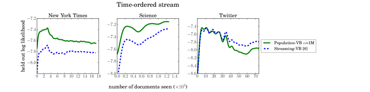
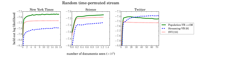
Figure 1: Held out predictive log likelihood for LDA on large-scale streamed text corpora. Population-VB outperforms existing methods for two out of the three settings. We use the best settings of $\alpha$.

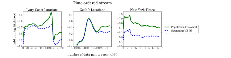
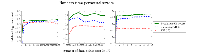
Figure 2: Held out predictive log likelihood for Dirichlet process mixture models on large-scale streamed location and text data sets. Note that we apply Gaussian likelihoods in the Geolife dataset, so the reported predictive performance is measured by probability density. We chose the best $\alpha$ for each population-VB curve

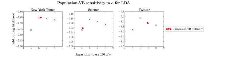
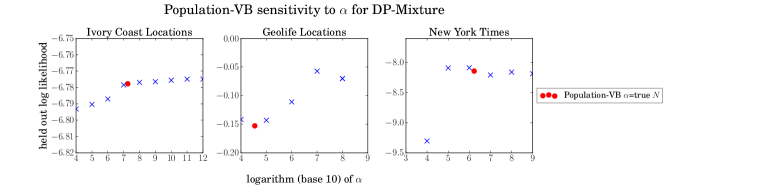
Figure 3: We show the sensitivity of population-VB to hyperparameter $\alpha$ (based on final log likelihoods in the time-ordered stream) and find that the best setting of $\alpha$ often differs from the true number of data points (which may not be known in any case in practice).

Datasets. With LDA we analyze three large-scale streamed corpora: 1.7M articles from the New York Times spanning 10 years, 130K Science articles written over 100 years, and 7.4M tweets collected from Twitter on Feb 2nd, 2014. We processed them all in a similar way, choosing a vocabulary based on the most frequent words in the corpus (with stop words removed): 8,000 for the New York Times, 5,855 for Science, and 13,996 for Twitter. On Twitter, we each tweet is a document, and we removed duplicate tweets and tweets that did not contain at least 2 words in the vocabulary.

With DP mixtures, we analyze human location behavior data. These data allow us to build periodic models of human population mobility, with applications to disaster response and urban planning. The Ivory Coast location data contains 18M discrete cell tower locations for 500K users recorded over 6 months [blondel_data_2012]. The Microsoft Geolife dataset contains 35K latitude-longitude GPS locations for 182 users over 5 years. For both data sets, our observations reflect down-sampling the data to ensure that each individual is seen no more than once every 15 minutes.

Results. We compare population VB with SVI [hoffman_stochastic_2013] and streaming variational Bayes (SVB) [broderick_streaming_2013] for LDA [broderick_streaming_2013] and DP mixtures [tank_streaming_2015]. SVB updates the variational approximation of the global parameter using sequential Bayesian updating, essentially accumulating expected sufficient statistics from minibatches of data observed in a stream. (Here we give the final results. We include the details of how we set and fit various hyperparameters below.)

We measure model fitness by evaluating the average predictive log likelihood on a set of held-out data. This involves splitting the observations of held-out data points into two equal halves, inferring the local component distribution based on the first half, and testing with the second half [hoffman_stochastic_2013]. For DP-mixtures, this works by predicting the location of a held-out data point by conditioning on the observed time of week.

In standard offline studies, the held-out set is randomly selected from the data. With streams, however, we test on the next 10K documents (for New York Times, Science), 500K tweets (for Twitter), or 25K locations (on Geo data). This is a valid held-out set because the data ahead of the current position in the stream have not yet been seen by the inference algorithms.

Figure 1 shows the performance of our algorithms for LDA. We looked at two types of streams: one in which the data appear in order and the other in which they have been permuted (i.e., an exchangeable stream). The time permuted stream reveals performance when each data minibatch is safely assumed to be an i.i.d. sample from $F$; this results in smoother improvements to predictive likelihood. On our data, we found that population VB outperformed SVI and SVB on two of the data sets and outperformed SVI on all of the data. SVB performed better than population VB on Twitter.

Figure 2 shows a similar study for DP mixtures. We analyzed the human mobility data and the New York Times. (Ref. [tank_streaming_2015] also analyzed the New York Times.) On these data population VB outperformed SVB and SVI in all settings.

Hyperparameters. Our methods are based on stochastic optimization and require setting the learning rate [nemirovski_robust_2009]. For all gradient-based procedures, we used a small fixed learning rate to follow noisy gradients. We note that adaptive learning rates [duchi_adaptive_2011, tieleman_lecture_2012] are also applicable in this setting, though we did not observe an improvement using these for time-ordered streams.

Our procedures also require setting a batch size, how many data points we observe before updating the approximate posterior. In the LDA study we set the batch size to 100 documents for the larger corpora (New York Times, Science) and 5,000 for Twitter. These sizes were selected to make the average number of words per batch equal in both settings, which helps lower the variance of the gradients. In the DP mixture study we use a batch size of 5,000 locations for Ivory Coast, 500 locations for Geolife, and 100 documents for New York Times.

Unlike traditional Bayesian methods, the data set size $\alpha$ is a hyperparameter to population VB. It helps control the posterior variance of the population posterior. Figure 3 reports sensitivity to $\alpha$ for all studies (for the time-ordered stream). These plots indicate that the optimal setting of $\alpha$ is often different from the true number of data points; the best performing population posterior variance is not necessarily the one implied by the data.

LDA requires additional hyperparameters. In line with [hoffman_structured_2015], we used 100 topics, and set the hyperparameter to the global topics (which controls the word sparsity of topics) to $\eta=0.01$ and the hyperparameter to the word-topic asssignments (which controls the sparsity of topic membership for each word) to $\gamma=0.1$. (We use these hyperparameters in Eq. 7 and Eq. 6.) The DP mixture model requires a truncation hyperparameter $K$, which we set to 100 for all three data sets and verified that the number of components used after inference was less than this limit.

4 Conclusions and Future Work

We introduced a new approach to modeling through the population posterior, a distribution over latent variables that combines traditional Bayesian inference and with the frequentist idea of the population distribution. With this idea, we derived population variational Bayes, an efficient algorithm for inference on streams. On two complex Bayesian models and several large data sets, we found that population variational Bayes usually performs better than existing approaches to streaming inference.

Appendix A Derivation and Bounds of the F-ELBO

Classic variational inference seeks to minimize $\mathrm{KL}(q(\beta,\mathbf{z})||p(\beta,\mathbf{z}\>|\>\mathbf{x}))$ using the following equivalence to show that the negative evidence lower bound (ELBO) is an appropriate surrogate objective to be minimized,

$$\log p(\mathbf{x}) = \mathrm{KL}(q(\beta,\mathbf{z})||p(\mathbf{z}\>|\>\mathbf{x}))+\mathbb{E}_{q}[\log p(\beta,\mathbf{z},\mathbf{x})-\log q(\beta,\mathbf{z})].$$ (11)

This equivalence arises from the definition of KL divergence [wainwright_graphical_2008].

To derive the F-ELBO, replace $\mathbf{x}$ with a draw $\mathbf{X}$ of size $\alpha$ from the population distribution, $\mathbf{X}\sim F_{\alpha}$, then apply an expectation with respect to $F_{\alpha}$ to both sides of Eq.11,

$$\mathbb{E}_{F_{\alpha}}[\log p(\mathbf{X})] = \mathbb{E}_{F_{\alpha}}[\mathrm{KL}(q(\beta,\mathbf{z})||p(\beta,\mathbf{z}\>|\>\mathbf{X}))+\mathbb{E}_{q}[\log p(\beta,\mathbf{z},\mathbf{X})-\log q(\beta,\mathbf{z})]]$$ (12)

$$= \mathbb{E}_{F_{\alpha}}[\mathrm{KL}(q(\beta,\mathbf{z})||p(\beta,\mathbf{z}\>|\>\mathbf{X}))]+\mathbb{E}_{F_{\alpha}}[\mathbb{E}_{q}[\log p(\beta,\mathbf{z},\mathbf{X})-\log q(\beta,\mathbf{z})]].$$

This confirms that the negative F-ELBO is a surrogate objective for $\mathbb{E}_{F_{\alpha}}[\mathrm{KL}(q(\beta,\mathbf{z})||p(\beta,\mathbf{z}\>|\>\mathbf{X}))]$ because $q(\cdot)$ does not appear on the left hand side of Eq. 12.

Now use the fact that logarithm is a concave function and apply Jensen’s inequality to Eq. 12 to show that the F-ELBO is a lower bound on the population evidence,

$$\mathbb{E}_{F_{\alpha}}[\mathbb{E}_{q}[\log p(\beta,\mathbf{z},\mathbf{X})-\log q(\beta,\mathbf{z})]] \leq \mathbb{E}_{F_{\alpha}}[\log p(\mathbf{X})]$$ (13)

$$\leq \log\mathbb{E}_{F_{\alpha}}[p(\mathbf{X})].$$

Additionally, Jensen’s inequality applied to Eq. 12 in a different way shows that maximizing the F-ELBO minimizes an upper bound on the KL divergence between $q(\cdot)$ and the population posterior,

$$\mathbb{E}_{F_{\alpha}}[\mathrm{KL}(q(\beta,\mathbf{z})||p(\beta,\mathbf{z}\>|\>\mathbf{X}))] = \mathbb{E}_{q}[\log q(\beta,\mathbf{z})]-\mathbb{E}_{F_{\alpha}}[\mathbb{E}_{q}[\log p(\beta,\mathbf{z}\>|\>\mathbf{X})]]$$ (14)

$$\geq \mathbb{E}_{q}[\log q(\beta,\mathbf{z})]-\mathbb{E}_{q}[\log\mathbb{E}_{F_{\alpha}}[p(\beta,\mathbf{z}\>|\>\mathbf{X})]]$$

$$= \mathrm{KL}(q(\beta,\mathbf{z})||\mathbb{E}_{F_{\alpha}}[p(\beta,\mathbf{z}\>|\>\mathbf{X})]),$$

where we have exchanged expectations with respect to $q(\cdot)$ and $F_{\alpha}$.

Appendix B One-Parameter F-ELBO

The F-ELBO for conditionally conjugate exponential families is as follows

$$\mathcal{L}(\lambda,\phi;F_{\alpha})=\mathbb{E}_{F_{\alpha}}\left[\mathbb{E}_{q}\left[\log p(\beta)-\log q(\beta\>|\>\lambda)+\sum_{i=1}^{\alpha}\log p(X_{i},Z_{i}\>|\>\beta)-\log q(Z_{i})]\right]\right].$$

This can be rewritten in terms of just the global variational parameters. We define the one parameter population variational inference objective as $\mathcal{L}_{F_{\alpha}}(\lambda)=\max_{\phi}\mathcal{L}_{F_{\alpha}}(\lambda,\phi)$. We can write this more compactly if we let $\phi_{i}(\lambda)$ be the value of $\phi_{i}$ that maximizes the F-ELBO given $\lambda$. Formally, this gives

$$\mathcal{L}_{F_{\alpha}}(\lambda)= \mathbb{E}_{q(\beta\>|\>\lambda)}\left[\log p(\beta)-\log q(\beta\>|\>\lambda)+\mathbb{E}_{\mathbf{X}\sim F_{\alpha}}[\sum_{i=1}^{\alpha}\mathbb{E}_{q(Z_{i}\>|\>\phi_{i}(\lambda))}\left[\log p(X_{i},Z_{i}\>|\>\beta)-\log q(Z_{i})]\right]\right],$$

where we have moved the expectation with respect to $F_{\alpha}$ inside the expectation with respect to $q(\cdot)$.

References

- [1] A. Ahmed, Q. Ho, C. H. Teo, J. Eisenstein, E. P. Xing, and A. J. Smola. Online inference for the infinite topic-cluster model: Storylines from streaming text. In International Conference on Artificial Intelligence and Statistics, pages 101–109, 2011.
- [2] S. I. Amari. Natural gradient works efficiently in learning. Neural Computation, 10(2):251–276, 1998.
- [3] J. M. Bernardo and A. F. Smith. Bayesian Theory, volume 405. John Wiley & Sons, 2009.
- [4] D. M. Blei, M. I. Jordan, et al. Variational inference for Dirichlet process mixtures. Bayesian Analysis, 1(1):121–143, 2006.
- [5] D. M. Blei, A. Y. Ng, and M. I. Jordan. Latent Dirichlet allocation. The Journal of Machine Learning Research, 3:993–1022, 2003.
- [6] V. D. Blondel, M. Esch, C. Chan, F. Clérot, P. Deville, E. Huens, F. Morlot, Z. Smoreda, and C. Ziemlicki. Data for development: the D4D challenge on mobile phone data. arXiv preprint arXiv:1210.0137, 2012.
- [7] L. Bottou. Online learning and stochastic approximations. Online learning in Neural Networks, 17:9, 1998.
- [8] T. Broderick, N. Boyd, A. Wibisono, A. C. Wilson, and M. Jordan. Streaming variational Bayes. In Advances in Neural Information Processing Systems, pages 1727–1735, 2013.
- [9] A. Doucet, S. Godsill, and C. Andrieu. On sequential Monte Carlo sampling methods for Bayesian filtering. Statistics and Computing, 10(3):197–208, 2000.
- [10] J. Duchi, E. Hazan, and Y. Singer. Adaptive subgradient methods for online learning and stochastic optimization. The Journal of Machine Learning Research, 12:2121–2159, 2011.
- [11] B. Efron and R. J. Tibshirani. An introduction to the bootstrap. CRC press, 1994.
- [12] M. D. Escobar and M. West. Bayesian density estimation and inference using mixtures. Journal of the American Statistical Association, 90(430):577–588, 1995.
- [13] Z. Ghahramani and H. Attias. Online variational Bayesian learning. In Slides from talk presented at NIPS 2000 Workshop on Online learning, pages 101–109, 2000.
- [14] M. D. Hoffman and D. M. Blei. Structured stochastic variational inference. In International Conference on Artificial Intelligence and Statistics, pages 101–109, 2015.
- [15] M. D. Hoffman, D. M. Blei, C. Wang, and J. Paisley. Stochastic variational inference. The Journal of Machine Learning Research, 14(1):1303–1347, 2013.
- [16] A. Honkela and H. Valpola. On-line variational Bayesian learning. In 4th International Symposium on Independent Component Analysis and Blind Signal Separation, pages 803–808, 2003.
- [17] M. I. Jordan, Z. Ghahramani, T. S. Jaakkola, and L. K. Saul. An introduction to variational methods for graphical models. Machine learning, 37(2):183–233, 1999.
- [18] D. P. Kingma and M. Welling. Auto-encoding variational Bayes. arXiv preprint arXiv:1312.6114, 2013.
- [19] A. Nemirovski, A. Juditsky, G. Lan, and A. Shapiro. Robust stochastic approximation approach to stochastic programming. SIAM Journal on Optimization, 19(4):1574–1609, 2009.
- [20] R. Ranganath, S. Gerrish, and D. M. Blei. Black box variational inference. In Proceedings of the Seventeenth International Conference on Artificial Intelligence and Statistics, pages 805–813, 2014.
- [21] H. Robbins and S. Monro. A stochastic approximation method. The Annals of Mathematical Statistics, pages 400–407, 1951.
- [22] L. K. Saul and M. I. Jordan. Exploiting tractable substructures in intractable networks. Advances in Neural Information Processing Systems, pages 486–492, 1996.
- [23] A. Tank, N. Foti, and E. Fox. Streaming variational inference for Bayesian nonparametric mixture models. In International Conference on Artificial Intelligence and Statistics, May 2015.
- [24] L. Theis and M. D. Hoffman. A trust-region method for stochastic variational inference with applications to streaming data. arXiv preprint arXiv:1505.07649, 2015.
- [25] T. Tieleman and G. Hinton. Lecture 6.5-RMSProp: Divide the gradient by a running average of its recent magnitude. COURSERA: Neural Networks for Machine Learning, 4, 2012.
- [26] M. Titsias and M. Lázaro-Gredilla. Doubly stochastic variational Bayes for non-conjugate inference. In Proceedings of the 31st International Conference on Machine Learning, pages 1971–1979, 2014.
- [27] M. J. Wainwright and M. I. Jordan. Graphical models, exponential families, and variational inference. Foundations and Trends in Machine Learning, 1(1-2):1–305, Jan. 2008.
- [28] L. Yao, D. Mimno, and A. McCallum. Efficient methods for topic model inference on streaming document collections. In Conference on Knowledge Discovery and Data Mining, pages 937–946. ACM, 2009.