\MakePerPage

footnote

Estimation of Space-Time Varying Parameters Using a Diffusion LMS Algorithm

Reza Abdolee,  Benoit Champagne,  and  Ali H. Sayed Copyright (c) 2013 IEEE. Personal use of this material is permitted. However, permission to use this material for any other purposes must be obtained from the IEEE by sending a request to pubs-permissions@ieee.org. R. Abdolee and B. Champagne are with the Department of Electrical and Computer Engineering, McGill University, Montreal, QC, H3A 2A7 Canada (e-mail: reza.abdolee@mail.mcgill.ca, benoit.champagne@mcgill.ca).A. H. Sayed is with the Department of Electrical Engineering, University of California, Los Angeles, CA 90095 USA (e-mail: sayed@ee.ucla.edu).The work of R. Abdolee and B. Champagne was supported by the Natural Sciences and Engineering Research Council (NSERC) of Canada. The work of A. H. Sayed was supported in part by NSF grant CCF-1011918.
Abstract

We study the problem of distributed adaptive estimation over networks where nodes cooperate to estimate physical parameters that can vary over both space and time domains. We use a set of basis functions to characterize the space-varying nature of the parameters and propose a diffusion least mean-squares (LMS) strategy to recover these parameters from successive time measurements. We analyze the stability and convergence of the proposed algorithm, and derive closed-form expressions to predict its learning behavior and steady-state performance in terms of mean-square error. We find that in the estimation of the space-varying parameters using distributed approaches, the covariance matrix of the regression data at each node becomes rank-deficient. Our analysis reveals that the proposed algorithm can overcome this difficulty to a large extent by benefiting from the network stochastic matrices that are used to combine exchanged information between nodes. We provide computer experiments to illustrate and support the theoretical findings.

Index Terms:
Diffusion adaptation, distributed processing, parameter estimation, space-varying parameters, sensor networks, interpolation.

I introduction

IN previous studies on diffusion algorithms for adaptation over networks, including least-mean-squares (LMS) or recursive least squares (RLS) types, the parameters being estimated are often assumed to be space-invariant [1, 2, 3, 4, 5, 6]. In other words, all agents are assumed to sense and measure data that arise from an underlying physical model that is represented by fixed parameters over the spatial domain. Some studies considered particular applications of diffusion strategies to data that arise from potentially different models [7, 8]. However, the proposed techniques in these works are not immediately applicable to scenarios where the estimation parameters vary over space across the network. This situation is encountered in many applications, including the monitoring of fluid flow in underground porous media [9], the tracking of population dispersal in ecology [10], the localization of distributed sources in dynamic systems [11], and the modeling of diffusion phenomena in inhomogeneous media [12]. In these applications, the space-varying parameters being estimated usually result from discretization of the coefficients of an underlying partial differential equation through spatial sampling.

The estimation of spatially-varying parameters has been addressed in several previous studies, including [13, 14, 15, 16, 17]. In these works and other similar references on the topic, the solutions typically rely on the use of a central processing (fusion) unit and less attention is paid to distributed and in-network processing solutions. Distributed algorithms are useful in large networks when there is no powerful fusion center and when the energy and communication resources of individual nodes are limited. Many different classes of distributed algorithms for parameter estimation over networks have been proposed in the recent literature, including incremental method[18, 19, 20, 21, 22], consensus methods [23, 24, 25, 26, 27, 28, 29, 30, 31, 32, 33, 34], and diffusion methods[35, 2, 3, 6, 36, 37]. Incremental techniques require to set-up a cyclic path between nodes over the network and are therefore sensitive to link failures. Consensus techniques require doubly-stochastic combination policies and can cause network instability in applications involving continuous adaptation and tracking [5]. In comparison, diffusion strategies demonstrate a stable behavior over networks regardless of the topology and endow networks with real-time adaptation and learning abilities [6, 36, 5].

Motivated by these considerations, in this paper, we develop a distributed LMS algorithm of the diffusion type to enable the estimation and tracking of parameters that may vary over both space and time. Our approach starts by introducing a linear regression model to characterize space-time varying phenomena over networks. This model is derived by discretizing a representative second-order partial differential equation (PDE), which can be useful in characterizing many dynamic systems with spatially-varying properties. We then introduce a set of basis functions, e.g., shifted Chebyshev polynomials, to represent the space-varying parameters of the underlying phenomena in terms of a finite set of space-invariant expansion coefficients. Building on this representation, we develop a diffusion LMS strategy that cooperatively estimates, interpolates, and tracks the model parameters over the network. We analyze the convergence and stability of the developed algorithm, and derive closed-form expressions to characterize the learning and convergence behavior of the nodes in mean-square-error sense. It turns out that in the context of space-time varying models, the covariance matrices of the regression data at the various nodes can become rank deficient. This property influences the learning behavior of the network and causes the estimates to become biased. We elaborate on how the judicious use of stochastic combination matrices can help alleviate this difficulty.

The paper is organized as follows. In Section II, we introduce a space-varying linear regression model which is motivated from a physical phenomenon characterized by a PDE, and formulate an optimization problem to find the unknown parameters of the introduced model. In Section III, we derive a diffusion LMS algorithm that solves this problem in a distributed and adaptive manner. We analyze the performance of the algorithm in Section IV, and present the numerical results of computer simulations in Section V. The concluding remarks appear in Section VI.

Notation: Matrices are represented by upper-case and vectors by lower-case letters. Boldface fonts are reserved for random variables and normal fonts are used for deterministic quantities. Superscript ()Tsuperscript𝑇(\cdot)^{T} denotes transposition for real-valued vectors and matrices and ()superscript(\cdot)^{\ast} denotes conjugate transposition for complex-valued vectors and matrices. The symbol \use@mathgroup\M@U\symAMSbE[]\use@mathgroup\M@U\symAMSb𝐸delimited-[]{\use@mathgroup\M@U\symAMSb{E}}[\cdot] is the expectation operator, Tr()Tr\text{Tr}(\cdot) represents the trace of its matrix argument and diag{}\{\cdot\} extracts the diagonal entries of a matrix, or constructs a diagonal matrix from a vector. IMsubscript𝐼𝑀I_{M} represents the identity matrix of size M×M𝑀𝑀M\times M (subscript M𝑀M is omitted when the size can be understood from the context). The vec()(\cdot) operator vectorizes a matrix by stacking its columns on top of each other. A set of vectors are stacked into a column vector by col{}col\mbox{\rm{col}}\{\cdot\}.

II Modeling and Problem Formulation

In this section, we motivate a linear regression model that can be used to describe dynamic systems with spatially varying properties. We derive the model from a representative second-order one-dimensional PDE that is used to characterize the evolution of the pressure distribution in inhomogeneous media and features a diffusion coefficient and an input source, both of which vary over space. Extension and generalization of the proposed approach, in modeling space-varying phenomena, to PDEs of higher order or defined over two-dimensional space are generally straightforward (see, e.g., Section V-C).

The PDE we consider is expressed as [12, 38]:

f(x,t)t=x(θ(x)f(x,t)x)+q(x,t)𝑓𝑥𝑡𝑡𝑥𝜃𝑥𝑓𝑥𝑡𝑥𝑞𝑥𝑡\displaystyle\frac{\partial f(x,t)}{\partial t}=\frac{\partial}{\partial x}\Bigg{(}\theta(x)\frac{\partial f(x,t)}{\partial x}\Bigg{)}+q(x,t) (1)

where (x,t)[0,L]×[0,T]𝑥𝑡0𝐿0𝑇(x,t)\in[0,L]\times[0,T] denote the space and time variables with upper limits L\use@mathgroup\M@U\symAMSbR+𝐿\use@mathgroup\M@U\symAMSbsuperscript𝑅L\in{\use@mathgroup\M@U\symAMSb R}^{+} and T\use@mathgroup\M@U\symAMSbR+𝑇\use@mathgroup\M@U\symAMSbsuperscript𝑅T\in{\use@mathgroup\M@U\symAMSb R}^{+}, respectively, f(x,t):\use@mathgroup\M@U\symAMSbR2\use@mathgroup\M@U\symAMSbR:𝑓𝑥𝑡\use@mathgroup\M@U\symAMSbsuperscript𝑅2\use@mathgroup\M@U\symAMSb𝑅f(x,t):{\use@mathgroup\M@U\symAMSb R}^{2}\rightarrow{\use@mathgroup\M@U\symAMSb R}, represents the system distribution (e.g., pressure or temperature) under study, θ(x):\use@mathgroup\M@U\symAMSbR\use@mathgroup\M@U\symAMSbR𝜃𝑥:\use@mathgroup\M@U\symAMSb𝑅\use@mathgroup\M@U\symAMSb𝑅\theta(x){\text{:}}\,{\use@mathgroup\M@U\symAMSb R}\rightarrow{\use@mathgroup\M@U\symAMSb R} is the space-varying diffusion coefficient and q(x,t):\use@mathgroup\M@U\symAMSbR2\use@mathgroup\M@U\symAMSbR𝑞𝑥𝑡:\use@mathgroup\M@U\symAMSbsuperscript𝑅2\use@mathgroup\M@U\symAMSb𝑅q(x,t){\text{:}}\,{\use@mathgroup\M@U\symAMSb R}^{2}\rightarrow{\use@mathgroup\M@U\symAMSb R} is the input distribution that includes sources and sinks. PDE (1) is assumed to satisfy the Dirichlet boundary conditions111Generalization of the boundary conditions to nonzero values is possible as well., f(0,t)=f(L,t)=0𝑓0𝑡𝑓𝐿𝑡0f(0,t)=f(L,t)=0 for all t[0,T]𝑡0𝑇t\in[0,T]. The distribution of the system at t=0𝑡0t=0 is given by f(x,0)=y(x)forx[0,L]𝑓𝑥0𝑦𝑥for𝑥0𝐿f(x,0)=y(x)\;\text{for}\;x\in[0,\,L]. It is convenient to rewrite (1) as:

f(x,t)t=θ(x)2f(x,t)x2+θ(x)xf(x,t)x+q(x,t)𝑓𝑥𝑡𝑡𝜃𝑥superscript2𝑓𝑥𝑡superscript𝑥2𝜃𝑥𝑥𝑓𝑥𝑡𝑥𝑞𝑥𝑡\displaystyle\frac{\partial f(x,t)}{\partial t}=\theta(x)\frac{{\partial}^{2}f(x,t)}{{\partial x}^{2}}+\frac{\partial\theta(x)}{\partial x}\frac{\partial f(x,t)}{\partial x}+q(x,t) (2)

and employ the finite difference method (FDM) to discretize the PDE over the time and space domains [39]. For N𝑁N and P𝑃P given positive integers, let Δx=L/(N+1)Δ𝑥𝐿𝑁1\Delta x=L/(N+1) and xk=kΔxsubscript𝑥𝑘𝑘Δ𝑥x_{k}=k\Delta x for k{0,1,2,,N+1}𝑘012𝑁1k\in\{0,1,2,\ldots,N+1\}, and similarly, let Δt=T/PΔ𝑡𝑇𝑃\Delta t=T/P and ti=iΔtsubscript𝑡𝑖𝑖Δ𝑡t_{i}=i\Delta t for i{0,1,2,,P}𝑖012𝑃i\in\{0,1,2,\ldots,P\}. We further introduce the sampled values of the pressure distribution fk(i)f(xk,ti)subscript𝑓𝑘𝑖𝑓subscript𝑥𝑘subscript𝑡𝑖f_{k}(i)\triangleq f(x_{k},t_{i}), input qk(i)q(xk,ti)subscript𝑞𝑘𝑖𝑞subscript𝑥𝑘subscript𝑡𝑖q_{k}(i)\triangleq q(x_{k},t_{i}), and space-varying coefficient θkθ(xk)subscript𝜃𝑘𝜃subscript𝑥𝑘\theta_{k}\triangleq\theta(x_{k}). It can be verified that applying FDM to (2), yields the following recursion:

fk(i)=uk,ihko+Δtqk(i1),k{1,2,,N}formulae-sequencesubscript𝑓𝑘𝑖subscript𝑢𝑘𝑖subscriptsuperscript𝑜𝑘Δ𝑡subscript𝑞𝑘𝑖1𝑘12𝑁f_{k}(i)={u}_{k,i}h^{o}_{k}+\Delta t\,q_{k}(i-1),\quad k\in\{1,2,\ldots,N\} (3)

where the vectors hko\use@mathgroup\M@U\symAMSbR3×1subscriptsuperscript𝑜𝑘\use@mathgroup\M@U\symAMSbsuperscript𝑅31h^{o}_{k}\in{\use@mathgroup\M@U\symAMSb R}^{3\times 1} and uk,i\use@mathgroup\M@U\symAMSbR1×3subscript𝑢𝑘𝑖\use@mathgroup\M@U\symAMSbsuperscript𝑅13{u}_{k,i}\in{\use@mathgroup\M@U\symAMSb R}^{1\times 3} are defined as

hko[h1,ko,h2,ko,h3,ko]Tsubscriptsuperscript𝑜𝑘superscriptsubscriptsuperscript𝑜1𝑘subscriptsuperscript𝑜2𝑘subscriptsuperscript𝑜3𝑘𝑇\displaystyle{h}^{o}_{k}\triangleq[h^{o}_{1,k},h^{o}_{2,k},h^{o}_{3,k}]^{T} (4)
uk,i[fk1(i1),fk(i1),fk+1(i1)]subscript𝑢𝑘𝑖subscript𝑓𝑘1𝑖1subscript𝑓𝑘𝑖1subscript𝑓𝑘1𝑖1\displaystyle{u}_{k,i}\triangleq[f_{k-1}(i-1),\,f_{k}(i-1),\,f_{k+1}(i-1)] (5)

the entries hm,ko\use@mathgroup\M@U\symAMSbRsubscriptsuperscript𝑜𝑚𝑘\use@mathgroup\M@U\symAMSb𝑅h^{o}_{m,k}\in{\use@mathgroup\M@U\symAMSb R} are:

h1,kosubscriptsuperscript𝑜1𝑘\displaystyle h^{o}_{1,k} =ν4(θk1+4θkθk+1)absent𝜈4subscript𝜃𝑘14subscript𝜃𝑘subscript𝜃𝑘1\displaystyle=\frac{\nu}{4}(\theta_{k-1}+4\theta_{k}-\theta_{k+1}) (6)
h2,kosubscriptsuperscript𝑜2𝑘\displaystyle h^{o}_{2,k} =12νθkabsent12𝜈subscript𝜃𝑘\displaystyle=1-2\nu\,\theta_{k} (7)
h3,kosubscriptsuperscript𝑜3𝑘\displaystyle h^{o}_{3,k} =ν4(θk1+4θk+θk+1)absent𝜈4subscript𝜃𝑘14subscript𝜃𝑘subscript𝜃𝑘1\displaystyle=\frac{\nu}{4}(-\theta_{k-1}+4\theta_{k}+\theta_{k+1}) (8)

and ν=Δt/Δx2𝜈Δ𝑡Δsuperscript𝑥2\nu={\Delta t}/{\Delta x^{2}}. Note that relation (3) is defined for k{1,2,,N}𝑘12𝑁k\in\{1,2,\cdots,N\}, i.e., no data sampling is required to be taken at x={0,L}𝑥0𝐿x=\{0,L\} because f0(i)subscript𝑓0𝑖f_{0}(i) and fN+1(i)subscript𝑓𝑁1𝑖f_{N+1}(i) respectively correspond to the known boundary conditions f(0,t)𝑓0𝑡f(0,t) and f(L,t)𝑓𝐿𝑡f(L,t). For monitoring purposes (e.g., estimation of θ(x)𝜃𝑥\theta(x)), sensor nodes collect noisy measurement samples of f(x,t)𝑓𝑥𝑡f(x,t) across the network. We denote these scalar measurement samples by

𝒛k(i)=fk(i)+𝒏k(i)subscript𝒛𝑘𝑖subscript𝑓𝑘𝑖subscript𝒏𝑘𝑖\boldsymbol{z}_{k}(i)=f_{k}(i)+\boldsymbol{n}_{k}(i) (9)

where 𝒏k(i)\use@mathgroup\M@U\symAMSbRsubscript𝒏𝑘𝑖\use@mathgroup\M@U\symAMSb𝑅\boldsymbol{n}_{k}(i)\in{\use@mathgroup\M@U\symAMSb R} is random noise term. Substituting (3) into (9) leads to

𝒅k(i)=uk,ihko+𝒏k(i)subscript𝒅𝑘𝑖subscript𝑢𝑘𝑖subscriptsuperscript𝑜𝑘subscript𝒏𝑘𝑖\boldsymbol{d}_{k}(i)=u_{k,i}h^{o}_{k}+\boldsymbol{n}_{k}(i) (10)

where

𝒅k(i)𝒛k(i)Δtqk(i1)subscript𝒅𝑘𝑖subscript𝒛𝑘𝑖Δ𝑡subscript𝑞𝑘𝑖1\boldsymbol{d}_{k}(i)\triangleq\boldsymbol{z}_{k}(i)-\Delta t\,q_{k}(i-1) (11)

The space-dependent model (10) can be generalized to accommodate higher order PDE’s, or to describe systems with more than one spatial dimension. In the generalized form, we assume that uk,isubscript𝑢𝑘𝑖u_{k,i} is random due to the possibility of sampling errors, and therefore represent it using boldface notation 𝒖k,isubscript𝒖𝑘𝑖\boldsymbol{u}_{k,i}. We also let hkosuperscriptsubscript𝑘𝑜h_{k}^{o} and 𝒖k,isubscript𝒖𝑘𝑖\boldsymbol{u}_{k,i} be M𝑀M-dimensional vectors. In addition, we denote the noise more generally by the symbol 𝒗k(i)subscript𝒗𝑘𝑖\boldsymbol{v}_{k}(i) to account for different sources of errors, including the measurement noise shown in (9) and modeling errors. Considering this generalization, the space-varying regression model that we shall consider is of the form:

𝒅k(i)=𝒖k,ihko+𝒗k(i)subscript𝒅𝑘𝑖subscript𝒖𝑘𝑖subscriptsuperscript𝑜𝑘subscript𝒗𝑘𝑖\boldsymbol{d}_{k}(i)=\boldsymbol{u}_{k,i}h^{o}_{k}+\boldsymbol{v}_{k}(i) (12)

where 𝒅k(i)\use@mathgroup\M@U\symAMSbR,𝒖k,i\use@mathgroup\M@U\symAMSbR1×M,hko\use@mathgroup\M@U\symAMSbRM×1formulae-sequencesubscript𝒅𝑘𝑖\use@mathgroup\M@U\symAMSb𝑅formulae-sequencesubscript𝒖𝑘𝑖\use@mathgroup\M@U\symAMSbsuperscript𝑅1𝑀subscriptsuperscript𝑜𝑘\use@mathgroup\M@U\symAMSbsuperscript𝑅𝑀1\boldsymbol{d}_{k}(i)\in{\use@mathgroup\M@U\symAMSb R},\boldsymbol{u}_{k,i}\in{\use@mathgroup\M@U\symAMSb R}^{1\times M},h^{o}_{k}\in{\use@mathgroup\M@U\symAMSb R}^{M\times 1} and 𝒗k(i)\use@mathgroup\M@U\symAMSbRsubscript𝒗𝑘𝑖\use@mathgroup\M@U\symAMSb𝑅\boldsymbol{v}_{k}(i)\in{\use@mathgroup\M@U\symAMSb R}. In this work, we study networks that monitor phenomena characterized by regression models of the form (12), where the objective is to estimate the space-varying parameter vectors hkosuperscriptsubscript𝑘𝑜h_{k}^{o} for k{1,2,,N}𝑘12𝑁k\in\{1,2,\cdots,N\}. In particular, we seek a distributed solution in the form of an adaptive algorithm with a diffusion mode of cooperation to enable the nodes to estimate and track these parameters over both space and time. The available information for estimation of the {hko}subscriptsuperscript𝑜𝑘\{h^{o}_{k}\} are the measurement samples, {𝒅k(i),𝒖k,i}subscript𝒅𝑘𝑖subscript𝒖𝑘𝑖\{\boldsymbol{d}_{k}(i),\boldsymbol{u}_{k,i}\}, collected at the N𝑁N spatial position xksubscript𝑥𝑘x_{k}, which we take to represent N𝑁N nodes.

Several studies, e.g., [13, 14, 15], solved space-varying parameter estimation problems using non-adaptive centralized techniques. In centralized optimization, the space-varying parameters {hko}subscriptsuperscript𝑜𝑘\{h^{o}_{k}\} are found by minimizing the following global cost function over the variables {hk}subscript𝑘\{h_{k}\}:

J(h1,,hN)k=1NJk(hk)𝐽subscript1subscript𝑁superscriptsubscript𝑘1𝑁subscript𝐽𝑘subscript𝑘J(h_{1},\ldots,h_{N})\triangleq\sum_{k=1}^{N}J_{k}(h_{k}) (13)

where

Jk(hk)\use@mathgroup\M@U\symAMSbE|𝒅k(i)𝒖k,ihk|2subscript𝐽𝑘subscript𝑘\use@mathgroup\M@U\symAMSb𝐸superscriptsubscript𝒅𝑘𝑖subscript𝒖𝑘𝑖subscript𝑘2J_{k}(h_{k})\triangleq{\use@mathgroup\M@U\symAMSb{E}}|\boldsymbol{d}_{k}(i)-\boldsymbol{u}_{k,i}h_{k}|^{2} (14)

To find hkosubscriptsuperscript𝑜𝑘h^{o}_{k} using distributed mechanisms, however, preliminary steps are required to transform the global cost (13) into a suitable form convenient for decentralized optimization [2]. Observe from (6)-(8) that collaborative processing is beneficial in this case because the hkosuperscriptsubscript𝑘𝑜h_{k}^{o} of neighboring nodes are related to each other through the space-dependent function θ(x)𝜃𝑥\theta(x).

Remark 1.

Note that if nodes individually estimate their own space-varying parameters by minimizing Jk(hk)subscript𝐽𝑘subscript𝑘J_{k}(h_{k}), then at each time instant, they will need to transmit their estimates to a fusion center for interpolation, in order to determine the value of the model parameters over regions of space where no measurements were collected. Using the proposed distributed algorithm in Section III-B, it will be possible to update the estimates and interpolate the results in a fully distributed manner. Cooperation also helps the nodes refine their estimates and perform more accurate interpolation. \blacksquare

III Adaptive Distributed Optimization

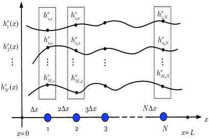
In distributed optimization over networked systems, nodes achieve their common objective through collaboration. Such an objective may be defined as finding a global parameter vector that minimizes a given cost function that encompasses the entire set of nodes. For the problem stated in this study, the unknown parameters in (13) are node-dependent. However, as we explained in Section II, these space-varying parameters are related through a well-defined function, e.g., θ(x)𝜃𝑥\theta(x) over the spatial domain. In the continuous space domain, the entries of each hkosubscriptsuperscript𝑜𝑘h^{o}_{k}, i.e., {h1,ko,,hM,ko}subscriptsuperscript𝑜1𝑘subscriptsuperscript𝑜𝑀𝑘\{h^{o}_{1,k},\cdots,h^{o}_{M,k}\} can be interpreted as samples of M𝑀M unknown space-varying parameter functions {h1o(x),,hMo(x)}subscriptsuperscript𝑜1𝑥subscriptsuperscript𝑜𝑀𝑥\{h^{o}_{1}(x),\cdots,h^{o}_{M}(x)\} at location x=xk𝑥subscript𝑥𝑘x=x_{k}, as illustrated in Fig. 1.

Refer to caption
Figure 1: An example of the space-varying parameter estimation problem over a one-dimensional network topology. The larger circles on the x𝑥x-axis represent the node locations at x=xk𝑥subscript𝑥𝑘x=x_{k}. These nodes collect samples {𝒅k(i),𝒖k,i}subscript𝒅𝑘𝑖subscript𝒖𝑘𝑖\{\boldsymbol{d}_{k}(i),\boldsymbol{u}_{k,i}\} to estimate the space-varying parameters {hko}subscriptsuperscript𝑜𝑘\{h^{o}_{k}\}. For simplicity in defining the vectors bksubscript𝑏𝑘b_{k} in (20), for this example, we assume that the node positions xksubscript𝑥𝑘x_{k} are uniformly spaced, however, generalization to non-uniform spacing is straightforward.

We can now use the well-established theory of interpolation to find a set of linear expansion coefficients, common to all the nodes, in order to estimate space-varying parameters using distributed optimization. Specifically, we assume that the m𝑚m-th unknown space-varying parameter function, hmo(x)subscriptsuperscript𝑜𝑚𝑥h^{o}_{m}(x) can be expressed as a unique linear combination of some Nbsubscript𝑁𝑏N_{b} space basis functions, i.e.,

hmo(x)=Wm,1b1(x)+Wm,2b2(x)++Wm,NbbNb(x)subscriptsuperscript𝑜𝑚𝑥subscript𝑊𝑚1subscript𝑏1𝑥subscript𝑊𝑚2subscript𝑏2𝑥subscript𝑊𝑚subscript𝑁𝑏subscript𝑏subscript𝑁𝑏𝑥h^{o}_{m}(x)=W_{m,1}b_{1}(x)+W_{m,2}b_{2}(x)+\cdots+W_{m,N_{b}}b_{N_{b}}(x) (15)

where {Wm,n}subscript𝑊𝑚𝑛\{W_{m,n}\} are the unique expansion coefficients and {bn(x)}subscript𝑏𝑛𝑥\{b_{n}(x)\} are the basis functions. In the application examples treated in Section V, we adopt shifted Chebyshev polynomials as basis functions, which are generated using the following expressions [40]

b1(x)=1,b2(x)=2x1formulae-sequencesubscript𝑏1𝑥1subscript𝑏2𝑥2𝑥1\displaystyle b_{1}(x)=1,\qquad b_{2}(x)=2x-1 (16)
bn+1(x)=2(2x1)bn(x)bn1(x),2<n<Nbformulae-sequencesubscript𝑏𝑛1𝑥22𝑥1subscript𝑏𝑛𝑥subscript𝑏𝑛1𝑥2𝑛subscript𝑁𝑏\displaystyle b_{n+1}(x)=2(2x-1)b_{n}(x)-b_{n-1}(x),\quad 2<n<N_{b} (17)

The choice of a suitable set of basis functions {bn(x)}n=1Nbsuperscriptsubscriptsubscript𝑏𝑛𝑥𝑛1subscript𝑁𝑏\{b_{n}(x)\}_{n=1}^{N_{b}} is application-specific and guided by multiple considerations such as representation efficiency, low computational complexity, interpolation capability, and other desirable properties, such as orthogonality. Chebyshev basis functions yield good results in terms of the above criteria and helps avoid the Runge’s phenomenon at the endpoints of the space interval [40].

The sampled version of the m𝑚m-th space-varying parameter hmo(x)subscriptsuperscript𝑜𝑚𝑥h^{o}_{m}(x) in (15), at x=xk=kΔx𝑥subscript𝑥𝑘𝑘Δ𝑥x=x_{k}=k\Delta x, can be written as:

hm,ko=WmTbksubscriptsuperscript𝑜𝑚𝑘superscriptsubscript𝑊𝑚𝑇subscript𝑏𝑘h^{o}_{m,k}=W_{m}^{T}b_{k} (18)

where

Wmsubscript𝑊𝑚\displaystyle W_{m} [Wm,1,Wm,2,,Wm,Nb]Tabsentsuperscriptsubscript𝑊𝑚1subscript𝑊𝑚2subscript𝑊𝑚subscript𝑁𝑏𝑇\displaystyle\triangleq[W_{m,1},W_{m,2},\cdots,W_{m,N_{b}}]^{T} (19)
bksubscript𝑏𝑘\displaystyle b_{k} [b1,k,,bNb,k]Tabsentsuperscriptsubscript𝑏1𝑘subscript𝑏subscript𝑁𝑏𝑘𝑇\displaystyle\triangleq[b_{1,k},\cdots,b_{N_{b},k}]^{T} (20)

and each entry bn,ksubscript𝑏𝑛𝑘b_{n,k} is obtained by sampling the corresponding basis function at the same location, i.e.,

bn,kbn(xk)=bn(kΔx)subscript𝑏𝑛𝑘subscript𝑏𝑛subscript𝑥𝑘subscript𝑏𝑛𝑘Δ𝑥b_{n,k}\triangleq b_{n}(x_{k})=b_{n}(k\Delta x) (21)

Collecting the sampled version of all M𝑀M functions hmo(x)superscriptsubscript𝑚𝑜𝑥h_{m}^{o}(x) for m{1,,M}𝑚1𝑀m\in\{1,\cdots,M\} into a column vector as

hko=[h1,ko,h2,ko,,hM,ko]Tsubscriptsuperscript𝑜𝑘superscriptsubscriptsuperscript𝑜1𝑘subscriptsuperscript𝑜2𝑘subscriptsuperscript𝑜𝑀𝑘𝑇h^{o}_{k}=[h^{o}_{1,k},h^{o}_{2,k},\cdots,h^{o}_{M,k}]^{T} (22)

and using (18), we arrive at:

hko=Wobksubscriptsuperscript𝑜𝑘superscript𝑊𝑜subscript𝑏𝑘h^{o}_{k}=W^{o}b_{k} (23)

where

Wo[W1,1oW1,2oW1,NboW2,1oW2,2oW2,NboWM,1oWM,2oWM,Nbo]superscript𝑊𝑜delimited-[]subscriptsuperscript𝑊𝑜11subscriptsuperscript𝑊𝑜12subscriptsuperscript𝑊𝑜1subscript𝑁𝑏subscriptsuperscript𝑊𝑜21subscriptsuperscript𝑊𝑜22subscriptsuperscript𝑊𝑜2subscript𝑁𝑏subscriptsuperscript𝑊𝑜𝑀1subscriptsuperscript𝑊𝑜𝑀2subscriptsuperscript𝑊𝑜𝑀subscript𝑁𝑏W^{o}\triangleq\left[\begin{array}[]{cccc}W^{o}_{1,1}&W^{o}_{1,2}&\ldots&W^{o}_{1,N_{b}}\\ W^{o}_{2,1}&W^{o}_{2,2}&\ldots&W^{o}_{2,N_{b}}\\ \vdots&\vdots&\ldots&\vdots\\ W^{o}_{M,1}&W^{o}_{M,2}&\ldots&W^{o}_{M,N_{b}}\end{array}\right] (24)
Remark 2.

Several other interpolation techniques can be used to obtain the basis functions bn(x)subscript𝑏𝑛𝑥b_{n}(x), such as the so-called kriging method [41]. The latter is a data-based weighting approach, rather than a distance-based interpolation. It is applicable in scenarios where the unknown random field to be interpolated, in our case hkosubscriptsuperscript𝑜𝑘h^{o}_{k}, is wide-sense stationary; accordingly, it requires knowledge about the means and covariances of the random field over space, as employed in [42]. If these covariances are not available, then the variogram models, describing the degree of spatial dependence of the random field, are used to generate substitutes for these covariances [43]. However, a-priori knowledge about the parameters of variogram models, including nugget, sill, and range, are required to obtain the spatial covariances. In this work, since neither the means and covariances nor the parameters of the variogram models of the random fields are available, we focus on interpolation techniques that rely on distance information rather than the statistics of the random field to be interpolated. \blacksquare

Returning to equation (23), it is convenient to rearrange Wosuperscript𝑊𝑜W^{o} into an MNb×1𝑀subscript𝑁𝑏1MN_{b}\times 1 column vector wosuperscript𝑤𝑜w^{o} by stacking up the columns of WoTsuperscriptsuperscript𝑊𝑜𝑇{W^{o}}^{T}, i.e., wo=vec(WoT)superscript𝑤𝑜vecsuperscriptsuperscript𝑊𝑜𝑇w^{o}={\rm{vec}}({W^{o}}^{T}), and defining the block diagonal matrix Bk\use@mathgroup\M@U\symAMSbRM×MNbsubscript𝐵𝑘\use@mathgroup\M@U\symAMSbsuperscript𝑅𝑀𝑀subscript𝑁𝑏B_{k}\in{\use@mathgroup\M@U\symAMSb R}^{M\times MN_{b}} as:

BkIMbkTsubscript𝐵𝑘tensor-productsubscript𝐼𝑀subscriptsuperscript𝑏𝑇𝑘B_{k}\triangleq I_{M}\otimes b^{T}_{k} (25)

Then, relation (23) can be rewritten in terms of the unique parameter vector wosuperscript𝑤𝑜w^{o} as:

hko=Bkwosubscriptsuperscript𝑜𝑘subscript𝐵𝑘superscript𝑤𝑜h^{o}_{k}=B_{k}w^{o} (26)

so that substituting hkosubscriptsuperscript𝑜𝑘h^{o}_{k} from (26) into (12) yields:

𝒅k(i)=𝒖k,iBkwo+𝒗k(i)subscript𝒅𝑘𝑖subscript𝒖𝑘𝑖subscript𝐵𝑘superscript𝑤𝑜subscript𝒗𝑘𝑖\displaystyle\boldsymbol{d}_{k}(i)=\boldsymbol{u}_{k,i}B_{k}w^{o}+\boldsymbol{v}_{k}(i) (27)

Subsequently, the global cost function (13) becomes:

J(w)=k=1N\use@mathgroup\M@U\symAMSbE|𝒅k(i)𝒖k,iBkw|2𝐽𝑤superscriptsubscript𝑘1𝑁\use@mathgroup\M@U\symAMSb𝐸superscriptsubscript𝒅𝑘𝑖subscript𝒖𝑘𝑖subscript𝐵𝑘𝑤2\displaystyle J(w)=\sum_{k=1}^{N}{\use@mathgroup\M@U\symAMSb{E}}|\boldsymbol{d}_{k}(i)-\boldsymbol{u}_{k,i}B_{k}w|^{2} (28)

In the following, we elaborate on how the parameter vector wosuperscript𝑤𝑜w^{o} and, hence, the {hko}superscriptsubscript𝑘𝑜\{h_{k}^{o}\} can be estimated from the data {𝒅k(i),𝒖k,i}subscript𝒅𝑘𝑖subscript𝒖𝑘𝑖\{\boldsymbol{d}_{k}(i),\boldsymbol{u}_{k,i}\} using centralized and distributed adaptive optimization.

III-A Centralized Adaptive Solution

We begin by stating the assumed statistical conditions on the data over the network.

Assumption 1.

We assume that {𝒅k(i),𝒖k,i,𝒗k(i)}subscript𝒅𝑘𝑖subscript𝒖𝑘𝑖subscript𝒗𝑘𝑖\{\boldsymbol{d}_{k}(i),\boldsymbol{u}_{k,i},\boldsymbol{v}_{k}(i)\} in model (27) satisfy the following conditions:

  1. 1.

    𝒅k(i)subscript𝒅𝑘𝑖\boldsymbol{d}_{k}(i) and 𝒖k,isubscript𝒖𝑘𝑖\boldsymbol{u}_{k,i} are zero-mean, jointly wide-sense stationary random processes with second-order moments:

    rdu,ksubscript𝑟𝑑𝑢𝑘\displaystyle r_{du,k} =\use@mathgroup\M@U\symAMSbE[𝒅k(i)𝒖k,iT]\use@mathgroup\M@U\symAMSbRM×1absent\use@mathgroup\M@U\symAMSb𝐸delimited-[]subscript𝒅𝑘𝑖superscriptsubscript𝒖𝑘𝑖𝑇\use@mathgroup\M@U\symAMSbsuperscript𝑅𝑀1\displaystyle={\use@mathgroup\M@U\symAMSb{E}}[\boldsymbol{d}_{k}(i)\boldsymbol{u}_{k,i}^{T}]\in{\use@mathgroup\M@U\symAMSb R}^{M\times 1} (29)
    Ru,ksubscript𝑅𝑢𝑘\displaystyle R_{u,k} =\use@mathgroup\M@U\symAMSbE[𝒖k,iT𝒖k,i]\use@mathgroup\M@U\symAMSbRM×Mabsent\use@mathgroup\M@U\symAMSb𝐸delimited-[]superscriptsubscript𝒖𝑘𝑖𝑇subscript𝒖𝑘𝑖\use@mathgroup\M@U\symAMSbsuperscript𝑅𝑀𝑀\displaystyle={\use@mathgroup\M@U\symAMSb{E}}[\boldsymbol{u}_{k,i}^{T}\boldsymbol{u}_{k,i}]\in{\use@mathgroup\M@U\symAMSb R}^{M\times M} (30)
  2. 2.

    The regression data {𝒖k,i}subscript𝒖𝑘𝑖\{\boldsymbol{u}_{k,i}\} are i.i.d. over time, independent over space, and their covariance matrices, Ru,ksubscript𝑅𝑢𝑘R_{u,k}, are positive definite for all k𝑘k.

  3. 3.

    The noise processes {𝒗k(i)}subscript𝒗𝑘𝑖\{\boldsymbol{v}_{k}(i)\} are zero-mean, i.i.d. over time, and independent over space with variances {σv,k2}subscriptsuperscript𝜎2𝑣𝑘\{\sigma^{2}_{v,k}\}.

  4. 4.

    The noise process 𝒗k(i)subscript𝒗𝑘𝑖\boldsymbol{v}_{k}(i) is independent of the regression data 𝒖m,jsubscript𝒖𝑚𝑗\boldsymbol{u}_{m,j} for all i,j𝑖𝑗i,j and k,m𝑘𝑚k,m. \blacksquare

The optimal parameter wosuperscript𝑤𝑜w^{o} that minimizes (28) can be found by setting the gradient vector of J(w)𝐽𝑤J(w) to zero. This yields the following normal equations:

(k=1NR¯u,k)wo=k=1Nr¯du,ksuperscriptsubscript𝑘1𝑁subscript¯𝑅𝑢𝑘superscript𝑤𝑜superscriptsubscript𝑘1𝑁subscript¯𝑟𝑑𝑢𝑘\Big{(}\sum_{k=1}^{N}\bar{R}_{u,k}\Big{)}w^{o}=\sum_{k=1}^{N}\bar{r}_{du,k} (31)

where {R¯u,k,r¯du,k}subscript¯𝑅𝑢𝑘subscript¯𝑟𝑑𝑢𝑘\{\bar{R}_{u,k},\bar{r}_{du,k}\} denote the second-order moments of 𝒖k,iBksubscript𝒖𝑘𝑖subscript𝐵𝑘\boldsymbol{u}_{k,i}B_{k} and 𝒅k(i)subscript𝒅𝑘𝑖\boldsymbol{d}_{k}(i):

R¯u,kBkTRu,kBk,r¯du,kBkTrdu,kformulae-sequencesubscript¯𝑅𝑢𝑘superscriptsubscript𝐵𝑘𝑇subscript𝑅𝑢𝑘subscript𝐵𝑘subscript¯𝑟𝑑𝑢𝑘superscriptsubscript𝐵𝑘𝑇subscript𝑟𝑑𝑢𝑘\bar{R}_{u,k}\triangleq B_{k}^{T}R_{u,k}B_{k},\;\;\;\;\bar{r}_{du,k}\triangleq B_{k}^{T}r_{du,k} (32)

It is clear from (31) that when k=1NR¯u,k>0superscriptsubscript𝑘1𝑁subscript¯𝑅𝑢𝑘0\sum_{k=1}^{N}\bar{R}_{u,k}>0, then wosuperscript𝑤𝑜w^{o} can be determined uniquely. If, on the other hand, k=1NR¯u,ksuperscriptsubscript𝑘1𝑁subscript¯𝑅𝑢𝑘\sum_{k=1}^{N}\bar{R}_{u,k} is singular, then we can use its pseudo-inverse to recover the minimum-norm solution of (31). Once the global solution is estimated, we can retrieve the space-varying parameter vectors hkosubscriptsuperscript𝑜𝑘h^{o}_{k} by substituting wosuperscript𝑤𝑜w^{o} into (26).

Alternatively the solution wosuperscript𝑤𝑜w^{o} of (31) can be sought iteratively by using the following steepest descent recursion:

𝒘i(c)=𝒘i1(c)+μk=1N(r¯du,kR¯u,k𝒘i1(c))subscriptsuperscript𝒘𝑐𝑖subscriptsuperscript𝒘𝑐𝑖1𝜇superscriptsubscript𝑘1𝑁subscript¯𝑟𝑑𝑢𝑘subscript¯𝑅𝑢𝑘subscriptsuperscript𝒘𝑐𝑖1\displaystyle\boldsymbol{w}^{(c)}_{i}=\boldsymbol{w}^{(c)}_{i-1}+\mu\sum_{k=1}^{N}\big{(}\bar{r}_{du,k}-\bar{R}_{u,k}\boldsymbol{w}^{(c)}_{i-1}\big{)} (33)

where μ>0𝜇0\mu>0 is a step-size parameter and 𝒘i(c)subscriptsuperscript𝒘𝑐𝑖\boldsymbol{w}^{(c)}_{i} is the estimate of wosuperscript𝑤𝑜w^{o} at the i𝑖i-th iteration. Recursion (33) requires the centralized processor to have knowledge of the covariance matrices, R¯u,ksubscript¯𝑅𝑢𝑘\bar{R}_{u,k}, and cross covariance vectors, r¯du,ksubscript¯𝑟𝑑𝑢𝑘\bar{r}_{du,k}, across all nodes. In practice, these moments are unknown in advance, and we therefore use their instantaneous approximations in (33). This substitution leads to the centralized LMS strategy (34)–(35) for space-varying parameter estimation over networks.

Algorithm 1 : Centralized LMS
𝒘i(c)=𝒘i1(c)+μk=1NBkT𝒖k,iT(𝒅k(i)𝒖k,iBk𝒘i1(c))subscriptsuperscript𝒘𝑐𝑖subscriptsuperscript𝒘𝑐𝑖1𝜇superscriptsubscript𝑘1𝑁superscriptsubscript𝐵𝑘𝑇superscriptsubscript𝒖𝑘𝑖𝑇subscript𝒅𝑘𝑖subscript𝒖𝑘𝑖subscript𝐵𝑘subscriptsuperscript𝒘𝑐𝑖1\displaystyle\boldsymbol{w}^{(c)}_{i}=\boldsymbol{w}^{(c)}_{i-1}+\mu\displaystyle\sum_{k=1}^{N}B_{k}^{T}\boldsymbol{u}_{k,i}^{T}\big{(}\boldsymbol{d}_{k}(i)-\boldsymbol{u}_{k,i}B_{k}\boldsymbol{w}^{(c)}_{i-1}\big{)} (34)
𝒉k,i=Bk𝒘i(c),k{1,2,,N}formulae-sequencesubscript𝒉𝑘𝑖subscript𝐵𝑘subscriptsuperscript𝒘𝑐𝑖𝑘12𝑁\displaystyle\boldsymbol{h}_{k,i}=B_{k}\boldsymbol{w}^{(c)}_{i},\quad k\in\{1,2,\cdots,N\} (35)

In this algorithm, at any given time instant i𝑖i, each node transmits its data {𝒖k,i,𝒅k(i)}subscript𝒖𝑘𝑖subscript𝒅𝑘𝑖\{\boldsymbol{u}_{k,i},\boldsymbol{d}_{k}(i)\} to the central processing unit to update 𝒘i1(c)subscriptsuperscript𝒘𝑐𝑖1\boldsymbol{w}^{(c)}_{i-1}. Subsequently, the algorithm obtains an estimate for the space-varying parameters, 𝒉k,isubscript𝒉𝑘𝑖\boldsymbol{h}_{k,i}, by using the updated estimate 𝒘i(c)subscriptsuperscript𝒘𝑐𝑖\boldsymbol{w}^{(c)}_{i}, and the basis function matrix at location k𝑘k, (i.e., Bksubscript𝐵𝑘B_{k}). This latter step can also be used as an interpolation mechanism to estimate the space-varying parameters at locations other than the pre-determined locations {xk}subscript𝑥𝑘\{x_{k}\}, by using the corresponding matrix B(x)𝐵𝑥B(x) for some desired location x𝑥x.

III-B Adaptive Diffusion Strategy

There are different distributed optimization techniques that can be applied to (28) in order to estimate wosuperscript𝑤𝑜w^{o} and consequently obtain the optimal space-varying parameters hkosubscriptsuperscript𝑜𝑘h^{o}_{k}. Let 𝒩ksubscript𝒩𝑘\mathcal{N}_{k} denote the index set of the neighbors of node k𝑘k, i.e., the nodes with which node k𝑘k can share information (including k𝑘k itself). One possible optimization strategy is to decouple the global cost (28) and write it as a set of constrained optimization problems with local variables wksubscript𝑤𝑘w_{k}, [44], i.e.,

minwk𝒩kc,k\use@mathgroup\M@U\symAMSbE|𝒅(i)𝒖,iBkwk|2subscriptsubscript𝑤𝑘subscriptsubscript𝒩𝑘subscript𝑐𝑘\use@mathgroup\M@U\symAMSb𝐸superscriptsubscript𝒅𝑖subscript𝒖𝑖subscript𝐵𝑘subscript𝑤𝑘2\displaystyle\min_{w_{k}}\sum_{\ell\in{\cal N}_{k}}c_{\ell,k}{\use@mathgroup\M@U\symAMSb{E}}|\boldsymbol{d}_{\ell}(i)-\boldsymbol{u}_{\ell,i}B_{k}w_{k}|^{2}
subject towk=wsubject tosubscript𝑤𝑘𝑤\displaystyle\text{subject to}\quad w_{k}=w (36)

where c,ksubscript𝑐𝑘c_{\ell,k} are nonnegative entries of a right-stochastic matrix C\use@mathgroup\M@U\symAMSbRN×N𝐶\use@mathgroup\M@U\symAMSbsuperscript𝑅𝑁𝑁C\in\use@mathgroup\M@U\symAMSb{R}^{N\times N} satisfying:

c,k=0if𝒩kandC𝟙=𝟙subscript𝑐𝑘0ifsubscript𝒩𝑘and𝐶double-struck-𝟙double-struck-𝟙\displaystyle c_{\ell,k}=0\;\,\text{if}\;\,\ell\notin\mathcal{N}_{k}\;\;\,\textrm{and}\;\;\;C{\mathbb{1}}={\mathbb{1}} (37)

and 𝟙double-struck-𝟙{\mathbb{1}} is the column vector with unit entries.

The optimization problem (36) can be solved using, for example, the alternating directions method of multipliers (ADMM) [45, 44]. In the algorithm derived using this method, the Lagrangian multipliers associated with the constraints need to be updated at every iteration during the optimization process. To this end, information about the network topology is required to establish a hierarchical communication structure between nodes. In addition, the constraints imposed by (36) require all agents to agree on an exact solution; this requirement degrades the learning and tracking abilities of the nodes over the network. When some nodes observe relevant data, it is advantageous for them to be able to respond quickly to the data without being critically constrained by perfect agreement at that stage. Doing so, would enable information to diffuse more rapidly across the network.

A technique that does not suffer from these difficulties and endows networks with adaptation and learning abilities in real-time is the diffusion strategy [35, 2, 3, 6, 36]. In this technique, minimizing the global cost (28) motivates solving the following unconstrained local optimization problem for k{1,,N}𝑘1𝑁k\in\{1,\cdots,N\} [2]:

minw(\displaystyle\min_{w}\Big{(} 𝒩kc,k\use@mathgroup\M@U\symAMSbE|𝒅(i)𝒖,iBkw|2subscriptsubscript𝒩𝑘subscript𝑐𝑘\use@mathgroup\M@U\symAMSb𝐸superscriptsubscript𝒅𝑖subscript𝒖𝑖subscript𝐵𝑘𝑤2\displaystyle\sum_{\ell\in{\cal N}_{k}}c_{\ell,k}{\use@mathgroup\M@U\symAMSb{E}}|\boldsymbol{d}_{\ell}(i)-\boldsymbol{u}_{\ell,i}B_{k}w|^{2}
+𝒩k\{k}p,kwψ2)\displaystyle\hskip 28.45274pt+\sum_{\ell\in{\cal N}_{k}\backslash\{k\}}p_{\ell,k}\|w-\psi_{\ell}\|^{2}\Big{)} (38)

where ψsubscript𝜓\psi_{\ell} is the available estimate of the global parameter at node \ell, 𝒩k\{k}\subscript𝒩𝑘𝑘{\cal N}_{k}\backslash\{k\} denotes set 𝒩ksubscript𝒩𝑘{\cal N}_{k} excluding node k𝑘k, and {p,k}subscript𝑝𝑘\{p_{\ell,k}\} are nonnegative scaling parameters. Following the arguments in [2, 3, 6], the minimization of (38) leads to a general form of the diffusion strategy described by (39)–(42), which can be specialized to several simpler yet useful forms.

Algorithm 2 : Diffusion LMS
ϕk,i1=𝒩ka,k(1)𝒘,i1subscriptbold-italic-ϕ𝑘𝑖1subscriptsubscript𝒩𝑘subscriptsuperscript𝑎1𝑘subscript𝒘𝑖1\displaystyle\mbox{\boldmath$\phi$}_{k,i-1}=\displaystyle\sum_{\ell\in\mathcal{N}_{k}}a^{(1)}_{\ell,k}\boldsymbol{w}_{\ell,i-1} (39)
𝝍k,i=ϕk,i1+μk𝒩kc,kBT𝒖,iT(𝒅(i)𝒖,iBϕk,i1)subscript𝝍𝑘𝑖subscriptbold-italic-ϕ𝑘𝑖1subscript𝜇𝑘subscriptsubscript𝒩𝑘subscript𝑐𝑘superscriptsubscript𝐵𝑇superscriptsubscript𝒖𝑖𝑇subscript𝒅𝑖subscript𝒖𝑖subscript𝐵subscriptbold-italic-ϕ𝑘𝑖1\displaystyle{\mbox{\boldmath$\psi$}}_{k,i}=\mbox{\boldmath$\phi$}_{k,i-1}+\mu_{k}\displaystyle\sum_{\ell\in\mathcal{N}_{k}}c_{\ell,k}B_{\ell}^{T}\boldsymbol{u}_{\ell,i}^{T}\big{(}\boldsymbol{d}_{\ell}(i)-\boldsymbol{u}_{\ell,i}B_{\ell}\mbox{\boldmath$\phi$}_{k,i-1}\big{)} (40)
𝒘k,i=𝒩ka,k(2)𝝍,isubscript𝒘𝑘𝑖subscriptsubscript𝒩𝑘subscriptsuperscript𝑎2𝑘subscript𝝍𝑖\displaystyle\boldsymbol{w}_{k,i}=\displaystyle\sum_{\ell\in\mathcal{N}_{k}}a^{(2)}_{\ell,k}{\mbox{\boldmath$\psi$}}_{\ell,i} (41)
𝒉k,i=Bk𝒘k,isubscript𝒉𝑘𝑖subscript𝐵𝑘subscript𝒘𝑘𝑖\displaystyle\boldsymbol{h}_{k,i}=B_{k}\boldsymbol{w}_{k,i} (42)

In this algorithm, μk>0subscript𝜇𝑘0\mu_{k}>0 is the step-size at node k𝑘k, {𝒘k,i,𝝍k,i,ϕk,i1}subscript𝒘𝑘𝑖subscript𝝍𝑘𝑖subscriptbold-italic-ϕ𝑘𝑖1\{\boldsymbol{w}_{k,i},\mbox{\boldmath$\psi$}_{k,i},\mbox{\boldmath$\phi$}_{k,i-1}\} are intermediate estimates of wosuperscript𝑤𝑜w^{o}, 𝒉k,isubscript𝒉𝑘𝑖\boldsymbol{h}_{k,i} is an intermediate estimate of hkosubscriptsuperscript𝑜𝑘h^{o}_{k}, and {a,k(1),a,k(2)}subscriptsuperscript𝑎1𝑘subscriptsuperscript𝑎2𝑘\{a^{(1)}_{\ell,k},a^{(2)}_{\ell,k}\} are nonnegative entries of left-stochastic matrices A1,A2\use@mathgroup\M@U\symAMSbRN×Nsubscript𝐴1subscript𝐴2\use@mathgroup\M@U\symAMSbsuperscript𝑅𝑁𝑁A_{1},A_{2}\in\use@mathgroup\M@U\symAMSb{R}^{N\times N} that satisfy:

a,k(1)=a,k(2)=0if𝒩kformulae-sequencesubscriptsuperscript𝑎1𝑘subscriptsuperscript𝑎2𝑘0ifsubscript𝒩𝑘\displaystyle a^{(1)}_{\ell,k}=a^{(2)}_{\ell,k}=0\quad\text{if}\,\ell\notin\mathcal{N}_{k} (43)
A1T𝟙=𝟙A2T𝟙=𝟙formulae-sequencesuperscriptsubscript𝐴1𝑇double-struck-𝟙double-struck-𝟙superscriptsubscript𝐴2𝑇double-struck-𝟙double-struck-𝟙\displaystyle\quad A_{1}^{T}{\mathbb{1}}={\mathbb{1}}\quad A_{2}^{T}{\mathbb{1}}={\mathbb{1}} (44)

Each node k𝑘k in the first combination step fuses {𝒘,i1}𝒩ksubscriptsubscript𝒘𝑖1subscript𝒩𝑘\{\boldsymbol{w}_{\ell,i-1}\}_{\ell\in{\cal N}_{k}} in a convex manner to generate ϕk,i1subscriptbold-italic-ϕ𝑘𝑖1\mbox{\boldmath$\phi$}_{k,i-1}. In the following step, named adaptation, each node k𝑘k uses its own data and that of neighboring nodes, i.e., {𝒖,i,𝒅(i)}𝒩ksubscriptsubscript𝒖𝑖subscript𝒅𝑖subscript𝒩𝑘\big{\{}\boldsymbol{u}_{\ell,i},\boldsymbol{d}_{\ell}(i)\big{\}}_{\ell\in{\cal N}_{k}} to adaptively update ϕk,i1subscriptbold-italic-ϕ𝑘𝑖1\mbox{\boldmath$\phi$}_{k,i-1} to an intermediate estimate 𝝍k,isubscript𝝍𝑘𝑖\mbox{\boldmath$\psi$}_{k,i}. In the third step, which is also a combination, the intermediate estimates {𝝍,i}𝒩ksubscriptsubscript𝝍𝑖subscript𝒩𝑘\{\mbox{\boldmath$\psi$}_{\ell,i}\}_{\ell\in\mathcal{N}_{k}} are fused to further align the global parameter estimate at node k𝑘k to that of its neighbors. Subsequently, the desired space-varying parameter 𝒉k,isubscript𝒉𝑘𝑖\boldsymbol{h}_{k,i} is obtained from 𝒘k,isubscript𝒘𝑘𝑖\boldsymbol{w}_{k,i}. Note that each step in the algorithm runs concurrently over the network.

Remark 3.

The main difference between Algorithm 2 and the previously developed diffusion LMS strategies in, e.g., [35, 2, 6] is in the transformed domain regression data 𝒖,iBsubscript𝒖𝑖subscript𝐵\boldsymbol{u}_{\ell,i}B_{\ell} in (40) which now have singular covariance matrices. Moreover, there is an additional interpolation step (42). \blacksquare

Remark 4.

The proposed diffusion LMS algorithm estimates NM𝑁𝑀NM spatially dependent variables {hko}superscriptsubscript𝑘𝑜\{h_{k}^{o}\} using NbMsubscript𝑁𝑏𝑀N_{b}M global invariant coefficients in wosuperscript𝑤𝑜w^{o}. From the computational complexity and energy efficiency point of view, it seems this is advantageous when the number of nodes, N𝑁N, is greater than the number of basis functions Nbsubscript𝑁𝑏N_{b}. However, even if this is not the case, using the estimated NbMsubscript𝑁𝑏𝑀N_{b}M global invariant coefficients, the algorithm not only can estimate the space-varying parameters at the locations of the N𝑁N nodes, but can also estimate the space-varying parameters at locations where no measurements are available. Therefore, even when N<Nb𝑁subscript𝑁𝑏N<N_{b}, the algorithm is still useful as it can perform interpolation. \blacksquare

There are different choices for the combination matrices {A1,A2,C}subscript𝐴1subscript𝐴2𝐶\{A_{1},A_{2},C\}. For example, the choice A1=A2=C=Isubscript𝐴1subscript𝐴2𝐶𝐼A_{1}=A_{2}=C=I reduces the above diffusion algorithm to the non-cooperative case where each node runs an individual LMS filter without coordination with its neighbors. Selecting C=I𝐶𝐼C=I simplifies the adaptation step (40) to the case where node k𝑘k uses only its own data {𝒅k(i),𝒖k,i}subscript𝒅𝑘𝑖subscript𝒖𝑘𝑖\{\boldsymbol{d}_{k}(i),\boldsymbol{u}_{k,i}\} to perform local adaptation. Choosing A1=Isubscript𝐴1𝐼A_{1}=I and A2=Asubscript𝐴2𝐴A_{2}=A, for some left-stochastic matrix A𝐴A, removes the first combination step and the algorithm reduces to an adaptation step followed by combination (this variant of the algorithm has the Adapt-then-Combine or ATC diffusion structure) [2, 6]. Likewise, choosing A1=Asubscript𝐴1𝐴A_{1}=A and A2=Isubscript𝐴2𝐼A_{2}=I removes the second combination step and the algorithm reduces to a combination step followed by adaptation (this variant has the Combine-then-Adapt (CTA) structure of diffusion [2, 6]). Often in practice, either the ATC or CTA version of the algorithm is used with C𝐶C set to C=I𝐶𝐼C=I such as using the following ATC diffusion version described by equations (45)–(47).

Algorithm 3 : Diffusion ATC
𝝍k,i=𝒘k,i1+μkBkT𝒖k,iT(𝒅k(i)𝒖k,iBk𝒘k,i1)subscript𝝍𝑘𝑖subscript𝒘𝑘𝑖1subscript𝜇𝑘superscriptsubscript𝐵𝑘𝑇superscriptsubscript𝒖𝑘𝑖𝑇subscript𝒅𝑘𝑖subscript𝒖𝑘𝑖subscript𝐵𝑘subscript𝒘𝑘𝑖1\displaystyle{\mbox{\boldmath$\psi$}}_{k,i}=\boldsymbol{w}_{k,i-1}+\mu_{k}B_{k}^{T}\boldsymbol{u}_{k,i}^{T}\big{(}\boldsymbol{d}_{k}(i)-\boldsymbol{u}_{k,i}B_{k}\boldsymbol{w}_{k,i-1}\big{)} (45)
𝒘k,i=𝒩ka,k𝝍,isubscript𝒘𝑘𝑖subscriptsubscript𝒩𝑘subscript𝑎𝑘subscript𝝍𝑖\displaystyle\boldsymbol{w}_{k,i}=\displaystyle\sum_{\ell\in\mathcal{N}_{k}}a_{\ell,k}{\mbox{\boldmath$\psi$}}_{\ell,i} (46)
𝒉k,i=Bk𝒘k,isubscript𝒉𝑘𝑖subscript𝐵𝑘subscript𝒘𝑘𝑖\displaystyle\boldsymbol{h}_{k,i}=B_{k}\boldsymbol{w}_{k,i} (47)

Nevertheless for generality, we shall study the performance of Algorithm 2 for arbitrary matrices {A1,A2,C}subscript𝐴1subscript𝐴2𝐶\{A_{1},A_{2},C\} with C𝐶C right-stochastic and {A1,A2}subscript𝐴1subscript𝐴2\{A_{1},A_{2}\} left-stochastic. The results can then be specialized to various situations of interest, including ATC, CTA, and the non-cooperative case.

The combination matrices {A1,A2,C}subscript𝐴1subscript𝐴2𝐶\{A_{1},A_{2},C\} are normally obtained using some well-known available combination rules such as the Metropolis or uniform combination rules [24, 35, 2]. These matrices can also be treated as free variables in the optimization procedure and used to further enhance the performance of the diffusion strategies. Depending on the network topology and the quality of the communication links between nodes, the optimized values of the combination matrices differ from one case to another[6, 46, 47, 48].

IV Performance Analysis

In this section, we analyze the performance of the diffusion strategy (39)-(42) in the mean and mean-square sense and derive expressions to characterize the network mean-square deviation (MSD) and excess mean-square error (EMSE). In the analysis, we need to consider the fact that the covariance matrices {R¯u,k}k=1Nsuperscriptsubscriptsubscript¯𝑅𝑢𝑘𝑘1𝑁\{\bar{R}_{u,k}\}_{k=1}^{N} defined in (32) are now rank-deficient since we have Nb>1subscript𝑁𝑏1N_{b}>1. We explain in the sequel the ramifications that follow from this rank-deficiency.

IV-A Mean Convergence

We introduce the local weight-error vectors

𝒘~k,iwo𝒘k,i,𝝍~k,iwo𝝍k,i,ϕ~k,iwoϕk,iformulae-sequencesubscript~𝒘𝑘𝑖superscript𝑤𝑜subscript𝒘𝑘𝑖formulae-sequencesubscript~𝝍𝑘𝑖superscript𝑤𝑜subscript𝝍𝑘𝑖subscript~bold-italic-ϕ𝑘𝑖superscript𝑤𝑜subscriptbold-italic-ϕ𝑘𝑖\tilde{\boldsymbol{w}}_{k,i}\triangleq w^{o}-\boldsymbol{w}_{k,i},\,\tilde{\mbox{\boldmath$\psi$}}_{k,i}\triangleq w^{o}-\mbox{\boldmath$\psi$}_{k,i},\,\tilde{\mbox{\boldmath$\phi$}}_{k,i}\triangleq w^{o}-\mbox{\boldmath$\phi$}_{k,i} (48)

and define the network error vectors:

ϕ~icol{ϕ~1,i,,ϕ~N,i}subscript~bold-italic-ϕ𝑖colsubscript~bold-italic-ϕ1𝑖subscript~bold-italic-ϕ𝑁𝑖\displaystyle\tilde{\mbox{\boldmath$\phi$}}_{i}\triangleq\mbox{\rm{col}}\{\tilde{\mbox{\boldmath$\phi$}}_{1,i},\ldots,\tilde{\mbox{\boldmath$\phi$}}_{N,i}\} (49)
𝝍~icol{𝝍~1,i,,𝝍~N,i}subscript~𝝍𝑖colsubscript~𝝍1𝑖subscript~𝝍𝑁𝑖\displaystyle\tilde{\mbox{\boldmath$\psi$}}_{i}\triangleq\mbox{\rm{col}}\{\tilde{\mbox{\boldmath$\psi$}}_{1,i},\ldots,\tilde{\mbox{\boldmath$\psi$}}_{N,i}\} (50)
𝒘~icol{𝒘~1,i,,𝒘~N,i}subscript~𝒘𝑖colsubscript~𝒘1𝑖subscript~𝒘𝑁𝑖\displaystyle\tilde{\boldsymbol{w}}_{i}\triangleq\mbox{\rm{col}}\{\tilde{\boldsymbol{w}}_{1,i},\ldots,\tilde{\boldsymbol{w}}_{N,i}\} (51)

We collect the estimates from across the network into the block vector:

𝒘icol{𝒘1,i,,𝒘N,i}subscript𝒘𝑖colsubscript𝒘1𝑖subscript𝒘𝑁𝑖\displaystyle\boldsymbol{w}_{i}\triangleq\mbox{\rm{col}}\{\boldsymbol{w}_{1,i},\ldots,\boldsymbol{w}_{N,i}\} (52)

and introduce the following extended combination matrices:

𝒜1subscript𝒜1\displaystyle{\mathcal{A}_{1}} A1IMNbabsenttensor-productsubscript𝐴1subscript𝐼𝑀subscript𝑁𝑏\displaystyle\triangleq A_{1}\otimes I_{MN_{b}} (53)
𝒜2subscript𝒜2\displaystyle{\mathcal{A}_{2}} A2IMNbabsenttensor-productsubscript𝐴2subscript𝐼𝑀subscript𝑁𝑏\displaystyle\triangleq A_{2}\otimes I_{MN_{b}} (54)
𝒞𝒞\displaystyle{\mathcal{C}} CIMNbabsenttensor-product𝐶subscript𝐼𝑀subscript𝑁𝑏\displaystyle\triangleq C\otimes I_{MN_{b}} (55)

We further define the block diagonal matrices and vectors:

𝓡isubscript𝓡𝑖\displaystyle\boldsymbol{\cal R}_{i} diag{𝒩kc,kBT𝒖,iT𝒖,iB:k=1,,N}absentdiagconditional-setsubscriptsubscript𝒩𝑘subscript𝑐𝑘superscriptsubscript𝐵𝑇superscriptsubscript𝒖𝑖𝑇subscript𝒖𝑖subscript𝐵𝑘1𝑁\displaystyle\triangleq\text{diag}\Big{\{}\small\sum_{\ell\in{\cal N}_{k}}c_{\ell,k}B_{\ell}^{T}\boldsymbol{u}_{\ell,i}^{T}\boldsymbol{u}_{\ell,i}B_{\ell}:k=1,\cdots,N\normalsize\Big{\}} (56)
\displaystyle{\mathcal{M}} diag{μ1IMNb,,μNIMNb}absentdiagsubscript𝜇1subscript𝐼𝑀subscript𝑁𝑏subscript𝜇𝑁subscript𝐼𝑀subscript𝑁𝑏\displaystyle\triangleq\text{diag}\big{\{}\mu_{1}I_{MN_{b}},\ldots,\mu_{N}I_{MN_{b}}\big{\}} (57)
𝒕isubscript𝒕𝑖\displaystyle\boldsymbol{t}_{i} col{𝒩kc,kBT𝒖,iT𝒅(i):k=1,,N}absentcolconditional-setsubscriptsubscript𝒩𝑘subscript𝑐𝑘superscriptsubscript𝐵𝑇superscriptsubscript𝒖𝑖𝑇subscript𝒅𝑖𝑘1𝑁\displaystyle\triangleq\mbox{\rm{col}}\Big{\{}\sum_{\ell\in{\cal N}_{k}}c_{\ell,k}B_{\ell}^{T}\boldsymbol{u}_{\ell,i}^{T}\boldsymbol{d}_{\ell}(i):k=1,\cdots,N\Big{\}} (58)
𝒈isubscript𝒈𝑖\displaystyle\boldsymbol{g}_{i} 𝒞Tcol{B1T𝒖1,iT𝒗1(i),,BNT𝒖N,iT𝒗N(i)}absentsuperscript𝒞𝑇colsuperscriptsubscript𝐵1𝑇superscriptsubscript𝒖1𝑖𝑇subscript𝒗1𝑖superscriptsubscript𝐵𝑁𝑇superscriptsubscript𝒖𝑁𝑖𝑇subscript𝒗𝑁𝑖\displaystyle\triangleq{\mathcal{C}}^{T}\,\mbox{\rm{col}}\big{\{}B_{1}^{T}\boldsymbol{u}_{1,i}^{T}\boldsymbol{v}_{1}(i),\cdots,B_{N}^{T}\boldsymbol{u}_{N,i}^{T}\boldsymbol{v}_{N}(i)\big{\}} (59)

and introduce the expected values of 𝓡isubscript𝓡𝑖\boldsymbol{\cal R}_{i} and 𝒕isubscript𝒕𝑖\boldsymbol{t}_{i}:

\use@mathgroup\M@U\symAMSbE[𝓡i]=diag{R1,,RN}\use@mathgroup\M@U\symAMSb𝐸delimited-[]subscript𝓡𝑖diagsubscript𝑅1subscript𝑅𝑁\displaystyle{\cal R}\triangleq{\use@mathgroup\M@U\symAMSb{E}}[\boldsymbol{\cal R}_{i}]=\text{diag}\big{\{}{R}_{1},\cdots,{R}_{N}\big{\}} (60)
r\use@mathgroup\M@U\symAMSbE[𝒕i]=col{r1,,rN}𝑟\use@mathgroup\M@U\symAMSb𝐸delimited-[]subscript𝒕𝑖colsubscript𝑟1subscript𝑟𝑁\displaystyle r\triangleq{\use@mathgroup\M@U\symAMSb{E}}[\boldsymbol{{t}}_{i}]=\mbox{\rm{col}}\big{\{}r_{1},\cdots,r_{N}\big{\}} (61)

where

Rk𝒩kc,kR¯u,subscript𝑅𝑘subscriptsubscript𝒩𝑘subscript𝑐𝑘subscript¯𝑅𝑢R_{k}\triangleq\sum_{\ell\in{\cal N}_{k}}c_{\ell,k}\,\bar{R}_{u,\ell} (62)
rk𝒩kc,kr¯du,subscript𝑟𝑘subscriptsubscript𝒩𝑘subscript𝑐𝑘subscript¯𝑟𝑑𝑢r_{k}\triangleq\sum_{\ell\in{\cal N}_{k}}c_{\ell,k}\,\bar{r}_{du,\ell} (63)

We also introduce an indicator matrix operator, denoted by Ind()Ind{\rm{Ind}}(\cdot), such that for any real-valued matrix X𝑋X with (k,j)𝑘𝑗(k,j)-th entry Xk,jsubscript𝑋𝑘𝑗X_{k,j}, the corresponding entry of Y=Ind(X)𝑌Ind𝑋Y={\rm{Ind}}(X) is:

Yk,j={1,ifXk,j>00,otherwisesubscript𝑌𝑘𝑗cases1ifsubscript𝑋𝑘𝑗0missing-subexpression0otherwisemissing-subexpressionY_{k,j}=\left\{\begin{array}[]{l l}1,\qquad\text{if}\;X_{k,j}>0\\ 0,\qquad\text{otherwise}\end{array}\right. (64)

Now from (39)–(41), we obtain:

𝒘i=𝓑i𝒘i1+𝒜2T𝒕isubscript𝒘𝑖subscript𝓑𝑖subscript𝒘𝑖1subscriptsuperscript𝒜𝑇2subscript𝒕𝑖\displaystyle\boldsymbol{w}_{i}=\boldsymbol{\mathcal{B}}_{i}\boldsymbol{w}_{i-1}+{\mathcal{A}}^{T}_{2}{\mathcal{M}}\boldsymbol{t}_{i} (65)

where

𝓑i𝒜2T(I𝓡i)𝒜1Tsubscript𝓑𝑖superscriptsubscript𝒜2𝑇𝐼subscript𝓡𝑖subscriptsuperscript𝒜𝑇1\boldsymbol{\mathcal{B}}_{i}\triangleq{\mathcal{A}}_{2}^{T}(I-{\mathcal{M}}\boldsymbol{\cal R}_{i}){\mathcal{A}}^{T}_{1} (66)

In turn, making use of (27) in (65), we can verify that the network error vector follows the recursion

𝒘~i=𝓑i𝒘~i1𝒜2T𝒈isubscript~𝒘𝑖subscript𝓑𝑖subscript~𝒘𝑖1superscriptsubscript𝒜2𝑇subscript𝒈𝑖\displaystyle\tilde{\boldsymbol{w}}_{i}=\boldsymbol{\mathcal{B}}_{i}\tilde{\boldsymbol{w}}_{i-1}-{\mathcal{A}}_{2}^{T}{\mathcal{M}}\boldsymbol{g}_{i} (67)

By taking the expectation of both sides of (67) and using Assumption 1, we arrive at:

\use@mathgroup\M@U\symAMSbE[𝒘~i]=\use@mathgroup\M@U\symAMSbE[𝒘~i1]\use@mathgroup\M@U\symAMSb𝐸delimited-[]subscript~𝒘𝑖\use@mathgroup\M@U\symAMSb𝐸delimited-[]subscript~𝒘𝑖1\displaystyle{\use@mathgroup\M@U\symAMSb{E}}[\tilde{\boldsymbol{w}}_{i}]={\cal B}\,{\use@mathgroup\M@U\symAMSb{E}}[\tilde{\boldsymbol{w}}_{i-1}] (68)

where in this relation:

\use@mathgroup\M@U\symAMSbE[𝓑i]=𝒜2T(I)𝒜1T\use@mathgroup\M@U\symAMSb𝐸delimited-[]subscript𝓑𝑖superscriptsubscript𝒜2𝑇𝐼subscriptsuperscript𝒜𝑇1\displaystyle{\cal B}\triangleq{\use@mathgroup\M@U\symAMSb{E}}[\boldsymbol{\mathcal{B}}_{i}]={\mathcal{A}}_{2}^{T}(I-{\mathcal{M}}{\cal R}){\mathcal{A}}^{T}_{1} (69)

To obtain (68), we used the fact that the expectation of the second term in (67), i.e., \use@mathgroup\M@U\symAMSbE[𝒜2T𝒈i]\use@mathgroup\M@U\symAMSb𝐸delimited-[]subscriptsuperscript𝒜𝑇2subscript𝒈𝑖{\use@mathgroup\M@U\symAMSb{E}}[{\mathcal{A}}^{T}_{2}{\mathcal{M}}\boldsymbol{g}_{i}], is zero because 𝒗k(i)subscript𝒗𝑘𝑖\boldsymbol{v}_{k}(i) is independent of 𝒖k,isubscript𝒖𝑘𝑖\boldsymbol{u}_{k,i} and \use@mathgroup\M@U\symAMSbE[𝒗k(i)]=0\use@mathgroup\M@U\symAMSb𝐸delimited-[]subscript𝒗𝑘𝑖0{\use@mathgroup\M@U\symAMSb{E}}[\boldsymbol{v}_{k}(i)]=0. The rank-deficient matrices {R¯u,k}subscript¯𝑅𝑢𝑘\{\bar{R}_{u,k}\} appear inside {\cal R} in (69). We now verify that despite having rank-deficient matrix {\cal R}, recursion (68) still guarantees a bounded mean error vector in steady-state.

To proceed, we introduce the eigendecomposition:

Rk=QkΛkQkTsubscript𝑅𝑘subscript𝑄𝑘subscriptΛ𝑘superscriptsubscript𝑄𝑘𝑇R_{k}=Q_{k}\Lambda_{k}Q_{k}^{T} (70)

where Qk=[qk,1,,qk,MNb]subscript𝑄𝑘subscript𝑞𝑘1subscript𝑞𝑘𝑀subscript𝑁𝑏Q_{k}=[q_{k,1},\cdots,q_{k,MN_{b}}] is a unitary matrix with column eigenvectors qk,jsubscript𝑞𝑘𝑗q_{k,j} and Λk=diag{λk(1),,λk(MNb)}subscriptΛ𝑘diagsubscript𝜆𝑘1subscript𝜆𝑘𝑀subscript𝑁𝑏\Lambda_{k}=\mbox{\rm{diag}}\{\lambda_{k}(1),\cdots,\lambda_{k}({MN_{b}})\} is a diagonal matrix with eigenvalues λk(j)0subscript𝜆𝑘𝑗0\lambda_{k}(j)\geq 0. For this decomposition, we assume that the eigenvalues of Rksubscript𝑅𝑘R_{k} are arranged in descending order, i.e, λmax(Rk)λk(1)λk(2)λk(MNb)subscript𝜆subscript𝑅𝑘subscript𝜆𝑘1subscript𝜆𝑘2subscript𝜆𝑘𝑀subscript𝑁𝑏\lambda_{\max}(R_{k})\triangleq\lambda_{k}(1)\geq\lambda_{k}(2)\geq\cdots\geq\lambda_{k}(MN_{b}), and the rank of Rksubscript𝑅𝑘R_{k} is LkMNbsubscript𝐿𝑘𝑀subscript𝑁𝑏L_{k}\leq MN_{b}. If we define 𝒬diag{Q1,,QN}𝒬diagsubscript𝑄1subscript𝑄𝑁{\cal Q}\triangleq\text{diag}\{Q_{1},\ldots,Q_{N}\} and Λdiag{Λ1,,ΛN}ΛdiagsubscriptΛ1subscriptΛ𝑁\Lambda\triangleq\mbox{\rm{diag}}\{\Lambda_{1},\cdots,\Lambda_{N}\}, then the network covariance matrix, {\cal R}, given by (60) can be expressed as:

=𝒬Λ𝒬T𝒬Λsuperscript𝒬𝑇{\cal R}={\cal Q}\Lambda{\cal Q}^{T} (71)

We now note that the mean estimate vector, \use@mathgroup\M@U\symAMSbE[𝒘~i]\use@mathgroup\M@U\symAMSb𝐸delimited-[]subscript~𝒘𝑖{\use@mathgroup\M@U\symAMSb{E}}[\tilde{\boldsymbol{w}}_{i}], expressed by (68) will be asymptotically unbiased if the spectral radius of {\cal B}, denoted by ρ()𝜌\rho({\cal B}), is strictly less than one. Let us examine under what conditions this requirement is satisfied. Since A1subscript𝐴1A_{1} and A2subscript𝐴2A_{2} are left-stochastic matrices and {\cal R} is block-diagonal, we have from [6] that:

ρ()=ρ(𝒜2T(I)𝒜1T)ρ(I)𝜌𝜌subscriptsuperscript𝒜𝑇2𝐼subscriptsuperscript𝒜𝑇1𝜌𝐼\rho({\cal B})=\rho\Big{(}{\cal A}^{T}_{2}(I-{\cal M}{\cal R}){\cal A}^{T}_{1}\Big{)}\leq\rho\big{(}I-{\cal M}{\cal R}\big{)} (72)

Therefore, if {\cal R} is positive-definite, then choosing μk<2/λmax(Rk)subscript𝜇𝑘2subscript𝜆subscript𝑅𝑘\mu_{k}<2/\lambda_{\max}(R_{k}) ensures convergence of the algorithm in the mean so that \use@mathgroup\M@U\symAMSbE[𝒘~i]0\use@mathgroup\M@U\symAMSb𝐸delimited-[]subscript~𝒘𝑖0{\use@mathgroup\M@U\symAMSb{E}}[\tilde{\boldsymbol{w}}_{i}]\rightarrow 0 as i𝑖i\rightarrow\infty. However, when {\cal R} is singular, it may hold that ρ()=1𝜌1\rho({\cal B})=1, in which case choosing the step-sizes according to the above bound guarantees the boundedness of the mean error, \use@mathgroup\M@U\symAMSbE[𝒘~i]\use@mathgroup\M@U\symAMSb𝐸delimited-[]subscript~𝒘𝑖{\use@mathgroup\M@U\symAMSb{E}}[\tilde{\boldsymbol{w}}_{i}], but not necessarily that it converges to zero. The following result clarifies these observations.

Theorem 1.

If the step-sizes are chosen to satisfy

0<μk<2λmax(Rk)0subscript𝜇𝑘2subscript𝜆subscript𝑅𝑘0<\mu_{k}<\frac{2}{\lambda_{\max}(R_{k})} (73)

then, under Assumption 1, the diffusion algorithm is stable in the mean in the following sense: (a) If ρ()<1𝜌1\rho({\cal B})<1, then \use@mathgroup\M@U\symAMSbE[𝒘~i]\use@mathgroup\M@U\symAMSb𝐸delimited-[]subscript~𝒘𝑖{\use@mathgroup\M@U\symAMSb{E}}[\tilde{\boldsymbol{w}}_{i}] converges to zero and (b) if ρ()=1𝜌1\rho({\cal B})=1 then

limi\use@mathgroup\M@U\symAMSbE[𝒘~i]b,subscript𝑖subscriptnorm\use@mathgroup\M@U\symAMSb𝐸delimited-[]subscript~𝒘𝑖𝑏\displaystyle\lim_{i\rightarrow\infty}\big{\|}{\use@mathgroup\M@U\symAMSb{E}}[{\tilde{\boldsymbol{w}}}_{i}]\big{\|}_{b,\infty} IInd(Λ)b,\use@mathgroup\M@U\symAMSbE[𝒘~1]b,absentsubscriptnorm𝐼IndΛ𝑏subscriptnorm\use@mathgroup\M@U\symAMSb𝐸delimited-[]subscript~𝒘1𝑏\displaystyle\leq\|I-{\rm{Ind}}(\Lambda)\|_{b,\infty}\,\big{\|}{\use@mathgroup\M@U\symAMSb{E}}[\tilde{\boldsymbol{w}}_{-1}]\big{\|}_{b,\infty} (74)

where b,\|\cdot\|_{b,\infty} stands for the block-maximum norm, as defined in [6, 47].

Proof.

See Appendix A.  ∎

In what follows, we examine recursion (65) and derive an expression for the asymptotic value of \use@mathgroup\M@U\symAMSbE[𝒘i]\use@mathgroup\M@U\symAMSb𝐸delimited-[]subscript𝒘𝑖{\use@mathgroup\M@U\symAMSb{E}}[\boldsymbol{w}_{i}]—see (89) further ahead. Before doing so, we first comment on a special case of interest, namely, result (76) below.

Special case: Consider a network with A1=A2=Isubscript𝐴1subscript𝐴2𝐼{A}_{1}={A}_{2}=I and an arbitrary right stochastic matrix C𝐶C satisfying (37). Using (27) and (62)-(63), it can be verified that the following linear system of equations holds at each node k𝑘k:

Rkwo=rksubscript𝑅𝑘superscript𝑤𝑜subscript𝑟𝑘R_{k}w^{o}=r_{k} (75)

We show in Appendix B that under condition (73) the mean estimate of the diffusion LMS algorithm at each node k𝑘k will converge to:

limi\use@mathgroup\M@U\symAMSbE[𝒘k,i]=Rkrk+n=Lk+1MNbqk,nqk,nT\use@mathgroup\M@U\symAMSbE[𝒘k,1]subscript𝑖\use@mathgroup\M@U\symAMSb𝐸delimited-[]subscript𝒘𝑘𝑖superscriptsubscript𝑅𝑘subscript𝑟𝑘superscriptsubscript𝑛subscript𝐿𝑘1𝑀subscript𝑁𝑏subscript𝑞𝑘𝑛superscriptsubscript𝑞𝑘𝑛𝑇\use@mathgroup\M@U\symAMSb𝐸delimited-[]subscript𝒘𝑘1\displaystyle\lim_{i\rightarrow\infty}{\use@mathgroup\M@U\symAMSb{E}}[\boldsymbol{w}_{k,i}]=R_{k}^{{\dagger}}r_{k}+\sum_{n={L_{k}+1}}^{MN_{b}}q_{k,n}q_{k,n}^{T}{\use@mathgroup\M@U\symAMSb{E}}[\boldsymbol{w}_{k,-1}] (76)

where Rksuperscriptsubscript𝑅𝑘R_{k}^{{\dagger}} represents the pseudo-inverse of Rksubscript𝑅𝑘R_{k}, and 𝒘k,1subscript𝒘𝑘1\boldsymbol{w}_{k,-1} is the node initial value. This result is consistent with the mean estimate of the stand-alone LMS filter with rank-deficient input data (which corresponds to the situation A1=A2=C=Isubscript𝐴1subscript𝐴2𝐶𝐼A_{1}=A_{2}=C=I)[49]. Note that Rkrksuperscriptsubscript𝑅𝑘subscript𝑟𝑘R_{k}^{{\dagger}}r_{k} in (76) corresponds to the minimum-norm solution of Rkw=rksubscript𝑅𝑘𝑤subscript𝑟𝑘R_{k}w=r_{k}. Therefore, the second term on the right hand side of (76) is the deviation of the node estimate from this minimum-norm solution. The presence of this term after convergence is due to the zero eigenvalues of Rksubscript𝑅𝑘R_{k}. If Rksubscript𝑅𝑘R_{k} were full-rank so that Lk=MNbsubscript𝐿𝑘𝑀subscript𝑁𝑏L_{k}=MN_{b}, then this term would disappear and the node estimate will converge, in the mean, to its optimal value, wosuperscript𝑤𝑜w^{o}. We point out that even though the matrices R¯u,subscript¯𝑅𝑢\bar{R}_{u,\ell} are rank deficient since Nb>1subscript𝑁𝑏1N_{b}>1, it is still possible for the matrices Rksubscript𝑅𝑘R_{k} to be full rank owing to the linear combination operation in (62). This illustrates one of the benefits of employing the right-stochastic matrix C𝐶C. However, if despite using C𝐶C, Rksubscript𝑅𝑘R_{k} still remains rank-deficient, the second term on the right-hand side of (76) can be annihilated by proper node initialization (e.g., by setting \use@mathgroup\M@U\symAMSbE[𝒘k,1]=0\use@mathgroup\M@U\symAMSb𝐸delimited-[]subscript𝒘𝑘10{\use@mathgroup\M@U\symAMSb{E}}[\boldsymbol{w}_{k,-1}]=0). By doing so, the mean estimate of each node will then approach the unique minimum-norm solution, Rkrksuperscriptsubscript𝑅𝑘subscript𝑟𝑘R_{k}^{{\dagger}}r_{k}.

General case: Let us now find the mean estimate of the network for arbitrary left-stochastic matrices A1subscript𝐴1A_{1} and A2subscript𝐴2A_{2}. Considering definitions (60)-(61) and relation (75) and noting that 𝒜1T(𝟙wo)=𝒜2T(𝟙wo)=(𝟙wo)subscriptsuperscript𝒜𝑇1tensor-productdouble-struck-𝟙superscript𝑤𝑜subscriptsuperscript𝒜𝑇2tensor-productdouble-struck-𝟙superscript𝑤𝑜tensor-productdouble-struck-𝟙superscript𝑤𝑜{\cal A}^{T}_{1}({\mathbb{1}}\otimes w^{o})={\cal A}^{T}_{2}({\mathbb{1}}\otimes w^{o})=({\mathbb{1}}\otimes w^{o}), it can be verified that (𝟙wo)tensor-productdouble-struck-𝟙superscript𝑤𝑜({\mathbb{1}}\otimes w^{o}) satisfies the following linear system of equations:

(I)(𝟙wo)=𝒜2Tr𝐼tensor-productdouble-struck-𝟙superscript𝑤𝑜subscriptsuperscript𝒜𝑇2𝑟\displaystyle(I-{\cal B})({\mathbb{1}}\otimes w^{o})={\mathcal{A}}^{T}_{2}{\mathcal{M}}r (77)

This is a useful intermediate result that will be applied in our argument.

Next, if we iterate recursion (65) and apply the expectation operator, we then obtain

\use@mathgroup\M@U\symAMSbE[𝒘i]=i+1\use@mathgroup\M@U\symAMSbE[𝒘1]+j=0ij𝒜2Tr\use@mathgroup\M@U\symAMSb𝐸delimited-[]subscript𝒘𝑖superscript𝑖1\use@mathgroup\M@U\symAMSb𝐸delimited-[]subscript𝒘1superscriptsubscript𝑗0𝑖superscript𝑗subscriptsuperscript𝒜𝑇2𝑟{\use@mathgroup\M@U\symAMSb{E}}[\boldsymbol{w}_{i}]={\mathcal{B}}^{i+1}{\use@mathgroup\M@U\symAMSb{E}}[\boldsymbol{w}_{-1}]+\sum_{j=0}^{i}{\cal B}^{j}{\cal A}^{T}_{2}{\mathcal{M}}r (78)

The mean estimate of the network can be found by computing the limit of this expression for i𝑖i\rightarrow\infty. To find the limit of the first term on the right hand side of (78), we evaluate limiisubscript𝑖superscript𝑖\lim_{i\rightarrow\infty}{\mathcal{B}}^{i} and find conditions under which it converges. For this purpose, we introduce the Jordan decomposition of matrix {\cal B} as [50]:

\displaystyle{\cal B} =𝒵Γ𝒵1absent𝒵Γsuperscript𝒵1\displaystyle={\cal Z}\Gamma{\cal Z}^{-1} (79)

where 𝒵𝒵{\cal Z} is an invertible matrix, and ΓΓ\Gamma is a block diagonal matrix of the form

Γ=diag{Γ1,Γ2,,Γs}ΓdiagsubscriptΓ1subscriptΓ2subscriptΓ𝑠\displaystyle\Gamma=\mbox{\rm{diag}}\Big{\{}\Gamma_{1},\Gamma_{2},\cdots,\Gamma_{s}\Big{\}} (80)

where the l𝑙l-th Jordan block, Γlml×mlsubscriptΓ𝑙superscriptsubscript𝑚𝑙subscript𝑚𝑙\Gamma_{l}\in{\mathbb{C}}^{m_{l}\times m_{l}}, can be expressed as:

Γl=γlIml+NmlsubscriptΓ𝑙subscript𝛾𝑙subscript𝐼subscript𝑚𝑙subscript𝑁subscript𝑚𝑙\Gamma_{l}=\gamma_{l}I_{m_{l}}+N_{m_{l}} (81)

In this relation, Nmlsubscript𝑁subscript𝑚𝑙N_{m_{l}} is some nilpotent matrix of size ml×mlsubscript𝑚𝑙subscript𝑚𝑙m_{l}\times m_{l}. Using decomposition (79), we can express isuperscript𝑖{\cal B}^{i} as

isuperscript𝑖\displaystyle{\mathcal{B}}^{i} =𝒵Γi𝒵1absent𝒵superscriptΓ𝑖superscript𝒵1\displaystyle={\cal Z}\Gamma^{i}{\cal Z}^{-1} (82)

Since ΓΓ\Gamma is block diagonal, we have

Γi=diag{Γ1i,Γ2i,,Γsi}superscriptΓ𝑖diagsuperscriptsubscriptΓ1𝑖superscriptsubscriptΓ2𝑖superscriptsubscriptΓ𝑠𝑖\displaystyle\Gamma^{i}=\mbox{\rm{diag}}\Big{\{}\Gamma_{1}^{i},\Gamma_{2}^{i},\cdots,\Gamma_{s}^{i}\Big{\}} (83)

From this relation, it is deduced that limiisubscript𝑖superscript𝑖\lim_{i\rightarrow\infty}{\cal B}^{i} exists if limiΓlisubscript𝑖superscriptsubscriptΓ𝑙𝑖\lim_{i\rightarrow\infty}\Gamma_{l}^{i} exists for all l{1,,s}𝑙1𝑠l\,\in\{1,\cdots,s\}. Using (81), we can write [50]:

limiΓli=limiγliml(γlmlIml+p=1ml1(ip)γlmlpNmlp)subscript𝑖superscriptsubscriptΓ𝑙𝑖subscript𝑖superscriptsubscript𝛾𝑙𝑖subscript𝑚𝑙superscriptsubscript𝛾𝑙subscript𝑚𝑙subscript𝐼subscript𝑚𝑙superscriptsubscript𝑝1subscript𝑚𝑙1binomial𝑖𝑝superscriptsubscript𝛾𝑙subscript𝑚𝑙𝑝superscriptsubscript𝑁subscript𝑚𝑙𝑝\displaystyle\lim_{i\rightarrow\infty}\Gamma_{l}^{i}=\lim_{i\rightarrow\infty}\gamma_{l}^{i-m_{l}}\Bigg{(}\gamma_{l}^{\scriptscriptstyle m_{l}}I_{m_{\scriptscriptstyle l}}+\sum_{p=1}^{m_{l}-1}\dbinom{i}{p}\gamma_{l}^{m_{l}-p}N_{\scriptscriptstyle m_{l}}^{p}\Bigg{)} (84)

When i𝑖{i\rightarrow\infty}, γlimlsuperscriptsubscript𝛾𝑙𝑖subscript𝑚𝑙\gamma_{l}^{i-m_{l}} becomes the dominant factor in this expression. Note that under condition (73), we have ρ()1𝜌1\rho({\cal B})\leq 1 which in turn implies that the magnitude of the eigenvalues of \cal B are bounded as 0|γn|10subscript𝛾𝑛10\leq|\gamma_{n}|\leq 1. Without loss of generality, we assume that the eigenvalues of {\cal B} are arranged as |γ1||γL|<|γL+1|==|γs|=1subscript𝛾1subscript𝛾𝐿subscript𝛾𝐿1subscript𝛾𝑠1|\gamma_{1}|\leq\cdots\leq|\gamma_{\scriptscriptstyle{L}}|<|\gamma_{\scriptscriptstyle{L+1}}|=\cdots=|\gamma_{s}|=1. Now we examine the limit (84) for every |γl|subscript𝛾𝑙|\gamma_{l}| in this range. Clearly for |γl|<1subscript𝛾𝑙1|\gamma_{l}|<1, the limit is zero (an obvious conclusion since in this case ΓlsubscriptΓ𝑙\Gamma_{l} is a stable matrix). For |γl|=1subscript𝛾𝑙1|\gamma_{l}|=1, the limit is the identity matrix if γl=1subscript𝛾𝑙1\gamma_{l}=1 and ml=1subscript𝑚𝑙1m_{l}=1. However, the limit does not exist for unit magnitude complex eigenvalues and eigenvalues with value -1, even when ml=1subscript𝑚𝑙1m_{l}=1. Motivated by these observations, we introduce the following definition.

Definition: We refer to matrix {\cal B} as power convergent if (a) its eigenvalues γnsubscript𝛾𝑛\gamma_{n} satisfy 0|γn|10subscript𝛾𝑛10\leq|\gamma_{n}|\leq 1, (b) its unit magnitude eigenvalues are all equal to one, and (c) its Jordan blocks associated with γn=1subscript𝛾𝑛1\gamma_{n}=1 are all of size 1×1111\times 1. \blacksquare

Example 1: Assume Nb=1subscript𝑁𝑏1N_{b}=1, Bk=IMsubscript𝐵𝑘subscript𝐼𝑀B_{k}=I_{M}, and uniform step-sizes and covariance matrices across the agents, i.e., μkμsubscript𝜇𝑘𝜇\mu_{k}\equiv\mu, Ru,kRusubscript𝑅𝑢𝑘subscript𝑅𝑢R_{u,k}\equiv R_{u} for all k𝑘k. Assume further that C𝐶C is doubly-stochastic (i.e., CT𝟙=𝟙=C𝟙)C^{T}{\mathbb{1}}={\mathbb{1}}=C{\mathbb{1}}) and Rusubscript𝑅𝑢R_{u} is singular. Then, in this case, the matrix {\cal B} can be written as the Kronecker product =A2TA1T(IMμRu)tensor-productsuperscriptsubscript𝐴2𝑇superscriptsubscript𝐴1𝑇subscript𝐼𝑀𝜇subscript𝑅𝑢{\cal B}=A_{2}^{T}A_{1}^{T}\otimes(I_{M}-\mu R_{u}). For strongly-connected networks where A1A2subscript𝐴1subscript𝐴2A_{1}A_{2} is a primitive matrix, it follows from the Perron-Frobenius Theorem [51] that A1A2subscript𝐴1subscript𝐴2A_{1}A_{2} has a single unit-magnitude eigenvalue at one, while all other eigenvalues have magnitude less than one. We conclude in this case, from the properties of Kronecker products and under condition (73), that {\cal B} is a power-convergent matrix. \blacksquare

Example 2: Assume M=2𝑀2M=2, N=3𝑁3N=3, Nb=1subscript𝑁𝑏1N_{b}=1, Bk=IMsubscript𝐵𝑘subscript𝐼𝑀B_{k}=I_{M}, and uniform step-sizes and covariance matrices across the agents again. Let A2=I=Csubscript𝐴2𝐼𝐶A_{2}=I=C and select

A1=A=[1/2001/201010]subscript𝐴1𝐴delimited-[]1200missing-subexpression1201missing-subexpression010missing-subexpressionA_{1}=A=\left[\begin{array}[]{cccc}1/2&0&0\\ 1/2&0&1\\ 0&1&0\end{array}\right] (85)

which is not primitive. Let further Ru=diag{β,0}subscript𝑅𝑢diag𝛽0R_{u}=\mbox{\rm diag}\{\beta,0\} denote a singular covariance matrix. Then, it can be verified in this case the corresponding matrix {\cal B} will have an eigenvalue with value 11-1 and is not power convergent. \blacksquare

Returning to the above definition and assuming {\cal B} is power convergent, then this means that the Jordan decomposition (79) can be rewritten as:

=[𝒵1𝒵2𝒵][J00I]Γ[𝒵¯1𝒵¯2]𝒵1delimited-[]subscriptsubscript𝒵1subscript𝒵2𝒵subscriptdelimited-[]𝐽00𝐼Γsubscriptdelimited-[]subscript¯𝒵1subscript¯𝒵2superscript𝒵1{\cal B}=[\underbrace{{\cal Z}_{1}\;{\cal Z}_{2}}_{\cal Z}]\underbrace{\left[\begin{array}[]{cc}J&0\\ 0&I\\ \end{array}\right]}_{\Gamma}\underbrace{\left[\begin{array}[]{c}\bar{\cal Z}_{1}\\ \bar{\cal Z}_{2}\\ \end{array}\right]}_{{\cal Z}^{-1}} (86)

where J𝐽J is a Jordan matrix with all eigenvalues strictly inside the unit circle, and the identity matrix inside ΓΓ\Gamma accounts for the eigenvalues with value one. In (86) we further partition 𝒵𝒵{\cal Z} and 𝒵1superscript𝒵1{\cal Z}^{-1} in accordance with the size of J𝐽J. Using (86), it is straightforward to verify that

limii+1subscript𝑖superscript𝑖1\displaystyle\lim_{i\rightarrow\infty}{\cal B}^{i+1} =𝒵2𝒵¯2absentsubscript𝒵2subscript¯𝒵2\displaystyle={\cal Z}_{2}{\bar{\cal Z}}_{2} (87)

and if we multiply both sides of (77) from the left by 𝒵¯2subscript¯𝒵2\bar{\cal Z}_{2}, it also follows that

𝒵¯2𝒜2Trsubscript¯𝒵2subscriptsuperscript𝒜𝑇2𝑟\displaystyle{\bar{\cal Z}}_{2}{\cal A}^{T}_{2}{\mathcal{M}}r =0absent0\displaystyle=0 (88)

Using these relations, we can now establish the following result, which describes the limiting behavior of the weight vector estimate.

Theorem 2.

If the step-sizes {μ1,,μN}subscript𝜇1subscript𝜇𝑁\{\mu_{1},\cdots,\mu_{N}\} satisfy (73) and matrix {\cal B} is power convergent, then the mean estimate of the network given by (78) asymptotically converges to:

limisubscript𝑖\displaystyle\lim_{i\rightarrow\infty} \use@mathgroup\M@U\symAMSbE[𝒘i]=(𝒵2𝒵¯2)\use@mathgroup\M@U\symAMSbE[𝒘1]+(I)𝒜2Tr\use@mathgroup\M@U\symAMSb𝐸delimited-[]subscript𝒘𝑖subscript𝒵2subscript¯𝒵2\use@mathgroup\M@U\symAMSb𝐸delimited-[]subscript𝒘1superscript𝐼subscriptsuperscript𝒜𝑇2𝑟\displaystyle{\use@mathgroup\M@U\symAMSb{E}}[\boldsymbol{w}_{i}]=({\cal Z}_{2}{\bar{\cal Z}}_{2})\,{\use@mathgroup\M@U\symAMSb{E}}[\boldsymbol{w}_{-1}]+(I-{\cal B})^{-}{\cal A}^{T}_{2}{\mathcal{M}}r (89)

where the notation Xsuperscript𝑋X^{-} denotes a (reflexive) generalized inverse for the matrix X𝑋X. In this case, the generalized inverse for I𝐼I-{\cal B} is given by

(I)=𝒵1(IJ)1𝒵¯1superscript𝐼subscript𝒵1superscript𝐼𝐽1subscript¯𝒵1(I-{\cal B})^{-}={\cal Z}_{1}(I-J)^{-1}\bar{{\cal Z}}_{1} (90)

which is in terms of the factors {𝒵1,𝒵¯1,J}subscript𝒵1subscript¯𝒵1𝐽\{{\cal Z}_{1},\bar{\cal Z}_{1},J\} defined in (86).

Proof.

See Appendix C.  ∎

We also argue in Appendix C that the quantity on the right-hand side of (89) is invariant under basis transformations for the Jordan factors {𝒵1,𝒵¯1,𝒵2,𝒵¯2}subscript𝒵1subscript¯𝒵1subscript𝒵2subscript¯𝒵2\{{\cal Z}_{1},\bar{\cal Z}_{1},{\cal Z}_{2},\bar{\cal Z}_{2}\}. It can be verified that if A1=A2=Isubscript𝐴1subscript𝐴2𝐼A_{1}=A_{2}=I then {\cal B} will be symmetric and the result (89) will reduce to (76). Now note that the first term on the right hand side of (89) is due to the zero eigenvalues of I𝐼I-{\cal B}. From this expression, we observe that different initialization values generally lead to different estimates. However, if we set \use@mathgroup\M@U\symAMSbE[𝒘1]=0\use@mathgroup\M@U\symAMSb𝐸delimited-[]subscript𝒘10{\use@mathgroup\M@U\symAMSb{E}}[\boldsymbol{w}_{-1}]=0, the algorithm converges to:

limi\use@mathgroup\M@U\symAMSbE[𝒘i]=(I)𝒜2Trsubscript𝑖\use@mathgroup\M@U\symAMSb𝐸delimited-[]subscript𝒘𝑖superscript𝐼subscriptsuperscript𝒜𝑇2𝑟\lim_{i\rightarrow\infty}{\use@mathgroup\M@U\symAMSb{E}}[\boldsymbol{w}_{i}]=(I-{\cal B})^{-}{\cal A}^{T}_{2}{\mathcal{M}}r (91)

In other words, the diffusion LMS algorithm will converge on average to a generalized inverse solution of the linear system of equations defined by (77).

When matrix {\cal B} is stable so that ρ()<1𝜌1\rho({\cal B})<1 then the factorization (86) reduces to the form =𝒵1J𝒵¯1subscript𝒵1𝐽subscript¯𝒵1{\cal B}={\cal Z}_{1}J{\bar{\cal Z}}_{1} and I𝐼I-{\cal B} will be full-rank. In that case, the first term on the right hand side of (89) will be zero and the generalized inverse will coincide with the actual matrix inverse so that (89) becomes

limisubscript𝑖\displaystyle\lim_{i\rightarrow\infty} \use@mathgroup\M@U\symAMSbE[𝒘i]=(I)1𝒜2Tr\use@mathgroup\M@U\symAMSb𝐸delimited-[]subscript𝒘𝑖superscript𝐼1subscriptsuperscript𝒜𝑇2𝑟\displaystyle{\use@mathgroup\M@U\symAMSb{E}}[\boldsymbol{w}_{i}]=(I-{\cal B})^{-1}{\cal A}^{T}_{2}{\mathcal{M}}r (92)

Comparing (92) with (77), we conclude that:

limisubscript𝑖\displaystyle\lim_{i\rightarrow\infty} \use@mathgroup\M@U\symAMSbE[𝒘i]=𝟙wo\use@mathgroup\M@U\symAMSb𝐸delimited-[]subscript𝒘𝑖tensor-productdouble-struck-𝟙superscript𝑤𝑜\displaystyle{\use@mathgroup\M@U\symAMSb{E}}[\boldsymbol{w}_{i}]={\mathbb{1}}\otimes w^{o} (93)

which implies that the mean estimate of each node will be wosuperscript𝑤𝑜w^{o}. This result is in agreement with the previously developed mean-convergence analysis of diffusion LMS when the regression data have full rank covariance matrices [6].

IV-B Mean-Square Error Convergence

We now examine the mean-square stability of the error recursion (67) in the rank-deficient scenario. We begin by deriving an error variance relation as in [52, 53]. To find this relation, we form the weighted square “norm” of (67), and compute its expectation to obtain:

\use@mathgroup\M@U\symAMSbE𝒘~iΣ2=\use@mathgroup\M@U\symAMSbE(𝒘~i1\displaystyle{\use@mathgroup\M@U\symAMSb{E}}\|\tilde{\boldsymbol{w}}_{i}\|^{2}_{\Sigma}={\use@mathgroup\M@U\symAMSb{E}}\big{(}\|\tilde{\boldsymbol{w}}_{i-1} 𝚺2)+\use@mathgroup\M@U\symAMSbE[𝒈iT𝒜2Σ𝒜2T𝒈i]\displaystyle\|^{2}_{{\boldsymbol{\Sigma}}^{\prime}}\big{)}+{\use@mathgroup\M@U\symAMSb{E}}[\boldsymbol{g}^{T}_{i}{\mathcal{M}}{\mathcal{A}_{2}}\Sigma{\mathcal{A}}^{T}_{2}{\mathcal{M}}\boldsymbol{g}_{i}] (94)

where xΣ2=xTΣxsubscriptsuperscriptnorm𝑥2Σsuperscript𝑥𝑇Σ𝑥\|x\|^{2}_{\Sigma}=x^{T}\Sigma x and Σ0Σ0\Sigma\geq 0 is an arbitrary weighting matrix of compatible dimension that we are free to choose. In this expression,

𝚺=𝒜1(I𝓡i)T𝒜2Σ𝒜2T(I𝓡i)𝒜1Tsuperscript𝚺subscript𝒜1superscript𝐼subscript𝓡𝑖𝑇subscript𝒜2Σsubscriptsuperscript𝒜𝑇2𝐼subscript𝓡𝑖subscriptsuperscript𝒜𝑇1\displaystyle{\boldsymbol{\Sigma}}^{\prime}={{\mathcal{A}_{1}}(I-{\mathcal{M}}\boldsymbol{\cal R}_{i})^{T}{\mathcal{A}_{2}}\Sigma{\mathcal{A}}^{T}_{2}(I-{\mathcal{M}}\boldsymbol{\cal R}_{i}){\mathcal{A}}^{T}_{1}} (95)

Under the temporal and spatial independence conditions on the regression data from Assumption 1, we can write:

\use@mathgroup\M@U\symAMSbE(𝒘~i1\displaystyle{\use@mathgroup\M@U\symAMSb{E}}\big{(}\|\tilde{\boldsymbol{w}}_{i-1} 𝚺2)=\use@mathgroup\M@U\symAMSbE𝒘~i12\use@mathgroup\M@U\symAMSbE[𝚺]\displaystyle\|^{2}_{{\boldsymbol{\Sigma}}^{\prime}}\big{)}={\use@mathgroup\M@U\symAMSb{E}}\|\tilde{\boldsymbol{w}}_{i-1}\|^{2}_{{\use@mathgroup\M@U\symAMSb{E}}[{\boldsymbol{\Sigma}}^{\prime}]} (96)

so that (94) becomes:

\use@mathgroup\M@U\symAMSbE𝒘~iΣ2=\use@mathgroup\M@U\symAMSbE𝒘~i1\use@mathgroup\M@U\symAMSb𝐸subscriptsuperscriptnormsubscript~𝒘𝑖2Σconditional\use@mathgroup\M@U\symAMSb𝐸subscript~𝒘𝑖1\displaystyle{\use@mathgroup\M@U\symAMSb{E}}\|\tilde{\boldsymbol{w}}_{i}\|^{2}_{\Sigma}={\use@mathgroup\M@U\symAMSb{E}}\|\tilde{\boldsymbol{w}}_{i-1} Σ2+Tr[Σ𝒜2T𝒢𝒜2]\displaystyle\|^{2}_{{\Sigma}^{\prime}}+{\rm{Tr}}[\Sigma{\mathcal{A}}^{T}_{2}{\mathcal{M}}{\mathcal{G}}{\mathcal{M}}{\mathcal{A}_{2}}] (97)

where 𝒢\use@mathgroup\M@U\symAMSbE[𝒈i𝒈iT]𝒢\use@mathgroup\M@U\symAMSb𝐸delimited-[]subscript𝒈𝑖subscriptsuperscript𝒈𝑇𝑖{\mathcal{G}}\triangleq{\use@mathgroup\M@U\symAMSb{E}}[{\boldsymbol{g}}_{i}{\boldsymbol{g}}^{T}_{i}] is given by

𝒢=𝒞Tdiag{σv,12R¯u,1,,σv,N2R¯u,N}𝒞𝒢superscript𝒞𝑇diagsubscriptsuperscript𝜎2𝑣1subscript¯𝑅𝑢1subscriptsuperscript𝜎2𝑣𝑁subscript¯𝑅𝑢𝑁𝒞\displaystyle{\mathcal{G}}={\mathcal{C}}^{T}\text{diag}\big{\{}\sigma^{2}_{v,1}\bar{R}_{u,1},\ldots,\sigma^{2}_{v,N}{\bar{R}}_{u,N}\big{\}}{\mathcal{C}} (98)

and

ΣsuperscriptΣ\displaystyle\Sigma^{\prime} \use@mathgroup\M@U\symAMSbE[𝚺]=TΣ+O(2)TΣabsent\use@mathgroup\M@U\symAMSb𝐸delimited-[]superscript𝚺superscript𝑇Σ𝑂superscript2superscript𝑇Σ\displaystyle\triangleq{\use@mathgroup\M@U\symAMSb{E}}[\boldsymbol{\Sigma}^{\prime}]={\cal B}^{T}\Sigma{\cal B}+O({\cal M}^{2})\approx{\cal B}^{T}\Sigma{\cal B} (99)

We shall employ (99) under the assumption of sufficiently small step-sizes where terms that depend on higher-order powers of the step-sizes are ignored. We next introduce

𝒴𝒜2T𝒢𝒜2𝒴subscriptsuperscript𝒜𝑇2𝒢subscript𝒜2{\cal Y}\triangleq{\cal A}^{T}_{2}{\cal M}{\cal G}{\cal M}{\cal A}_{2} (100)

and use (97) to write:

\use@mathgroup\M@U\symAMSbE𝒘~iΣ2=\use@mathgroup\M@U\symAMSbE𝒘~i1Σ2+Tr(Σ𝒴)\use@mathgroup\M@U\symAMSb𝐸subscriptsuperscriptnormsubscript~𝒘𝑖2Σ\use@mathgroup\M@U\symAMSb𝐸subscriptsuperscriptnormsubscript~𝒘𝑖12superscriptΣTrΣ𝒴\displaystyle{\use@mathgroup\M@U\symAMSb{E}}\|{\tilde{\boldsymbol{w}}}_{i}\|^{2}_{\Sigma}={\use@mathgroup\M@U\symAMSb{E}}\|{\tilde{\boldsymbol{w}}}_{i-1}\|^{2}_{\Sigma^{\prime}}+{\rm{Tr}}(\Sigma{\cal Y}) (101)

From (101), we arrive at

\use@mathgroup\M@U\symAMSbE𝒘~iΣ2=\use@mathgroup\M@U\symAMSb𝐸superscriptsubscriptnormsubscript~𝒘𝑖Σ2absent\displaystyle{\use@mathgroup\M@U\symAMSb{E}}\|{\tilde{\boldsymbol{w}}}_{i}\|_{\Sigma}^{2}= \use@mathgroup\M@U\symAMSbE𝒘~1(T)i+1Σi+12+j=0iTr((T)jΣj𝒴)\use@mathgroup\M@U\symAMSb𝐸subscriptsuperscriptnormsubscript~𝒘12superscriptsuperscript𝑇𝑖1Σsuperscript𝑖1superscriptsubscript𝑗0𝑖Trsuperscriptsuperscript𝑇𝑗Σsuperscript𝑗𝒴\displaystyle{\use@mathgroup\M@U\symAMSb{E}}\|\tilde{\boldsymbol{w}}_{-1}\|^{2}_{({\cal B}^{T})^{i+1}\Sigma{\cal B}^{i+1}}+\sum_{j=0}^{i}{\rm{Tr}}\Big{(}({\cal B}^{T})^{j}\Sigma{\cal B}^{j}{\cal Y}\Big{)} (102)

To prove the convergence and stability of the algorithm in the mean-square sense, we examine the convergence of the terms on the right hand side of (102).

In a manner similar to (88), it is shown in Appendix D that the following property holds:

𝒵¯2𝒴=0,𝒴𝒵¯2T=0formulae-sequencesubscript¯𝒵2𝒴0𝒴superscriptsubscript¯𝒵2𝑇0\bar{\cal Z}_{2}{\cal Y}=0,\;\;\;\;\;{\cal Y}\bar{\cal Z}_{2}^{T}=0 (103)

Exploiting this result, we can arrive at the following statement, which establishes that relation (102) converges as i𝑖i\rightarrow\infty and determines its limiting value.

Theorem 3.

Assume the step-sizes are sufficiently small and satisfy (73). Assume also that {\cal B} is power convergent. Under these conditions, relation (102) converges to

limi\use@mathgroup\M@U\symAMSbE𝒘~iΣ2subscript𝑖\use@mathgroup\M@U\symAMSb𝐸subscriptsuperscriptnormsubscript~𝒘𝑖2Σ\displaystyle\lim_{i\rightarrow\infty}{\use@mathgroup\M@U\symAMSb{E}}\|{\tilde{\boldsymbol{w}}}_{i}\|^{2}_{\Sigma} =\use@mathgroup\M@U\symAMSbE𝒘~1(𝒵2𝒵¯2)TΣ𝒵2𝒵¯22absent\use@mathgroup\M@U\symAMSb𝐸subscriptsuperscriptnormsubscript~𝒘12superscriptsubscript𝒵2subscript¯𝒵2𝑇Σsubscript𝒵2subscript¯𝒵2\displaystyle={\use@mathgroup\M@U\symAMSb{E}}\|\tilde{\boldsymbol{w}}_{-1}\|^{2}_{({\cal Z}_{2}\bar{\cal Z}_{2})^{T}\Sigma{\cal Z}_{2}\bar{\cal Z}_{2}}
+(vec(𝒴))T(I)1vec(Σ)superscriptvec𝒴𝑇superscript𝐼1vecΣ\displaystyle\qquad+\big{(}{\rm{vec}}({\cal Y})\big{)}^{T}(I-{\cal F})^{-1}{\rm{vec}}(\Sigma) (104)

where

((𝒵1𝒵1)(JJ)(𝒵¯1𝒵¯1))Tsuperscripttensor-productsubscript𝒵1subscript𝒵1tensor-product𝐽𝐽tensor-productsubscript¯𝒵1subscript¯𝒵1𝑇{\cal F}\triangleq\big{(}({\cal Z}_{1}\otimes{\cal Z}_{1})(J\otimes J)({\bar{\cal Z}_{1}}\otimes{\bar{\cal Z}_{1}})\big{)}^{T} (105)

and factors {𝒵1,𝒵¯1,J}subscript𝒵1subscript¯𝒵1𝐽\{{\cal Z}_{1},\bar{\cal Z}_{1},J\} are defined in (86).

Proof.

See Appendix D.  ∎

In a manner similar to the proof at the end of Appendix C, the term on the right hand side of (104) is invariant under basis transformations on the factors {𝒵1,𝒵¯1,𝒵2,𝒵¯2}subscript𝒵1subscript¯𝒵1subscript𝒵2subscript¯𝒵2\{{\cal Z}_{1},\bar{\cal Z}_{1},{\cal Z}_{2},\bar{\cal Z}_{2}\}. Note that the first term on the right hand side of (104) is the network penalty due to rank-deficiency. When the node covariance matrices are full rank, then choosing step-sizes according to (73) leads to ρ()<1𝜌1\rho({\cal B})<1. When this holds, then =𝒵1J𝒵¯1subscript𝒵1𝐽subscript¯𝒵1{\cal B}={\cal Z}_{1}J\bar{\cal Z}_{1}. In this case, the first term on the right hand side of (104) will be zero, and =()Tsuperscripttensor-product𝑇{\cal F}=({\cal B}\otimes{\cal B})^{T}. In this case, we obtain:

limi\use@mathgroup\M@U\symAMSbE𝒘~iΣ2=(vec(𝒴))T(I)1vec(Σ)subscript𝑖\use@mathgroup\M@U\symAMSb𝐸subscriptsuperscriptnormsubscript~𝒘𝑖2Σsuperscriptvec𝒴𝑇superscript𝐼1vecΣ\displaystyle\lim_{i\rightarrow\infty}{\use@mathgroup\M@U\symAMSb{E}}\|{\tilde{\boldsymbol{w}}}_{i}\|^{2}_{\Sigma}=\big{(}{\rm{vec}}({\cal Y})\big{)}^{T}(I-{\cal F})^{-1}{\rm{vec}}(\Sigma) (106)

which is in agreement with the mean-square analysis of diffusion LMS strategies for regression data with full rank covariance matrices given in [2, 6].

IV-C Learning Curves

For each k𝑘k, the MSD and EMSE measures are defined as:

ηksubscript𝜂𝑘\displaystyle\eta_{k} =limi\use@mathgroup\M@U\symAMSbE𝒉~k,i2=limi\use@mathgroup\M@U\symAMSbE𝒘~k,iBkTBk2absentsubscript𝑖\use@mathgroup\M@U\symAMSb𝐸superscriptnormsubscript~𝒉𝑘𝑖2subscript𝑖\use@mathgroup\M@U\symAMSb𝐸subscriptsuperscriptnormsubscript~𝒘𝑘𝑖2superscriptsubscript𝐵𝑘𝑇subscript𝐵𝑘\displaystyle=\lim_{i\rightarrow\infty}{\use@mathgroup\M@U\symAMSb{E}}\|\tilde{\boldsymbol{h}}_{k,i}\|^{2}=\lim_{i\rightarrow\infty}{\use@mathgroup\M@U\symAMSb{E}}\|\tilde{\boldsymbol{w}}_{k,i}\|^{2}_{B_{k}^{T}B_{k}} (107)
ζksubscript𝜁𝑘\displaystyle\zeta_{k} =limi\use@mathgroup\M@U\symAMSbE𝒖k,i𝒉~k,i12=limi\use@mathgroup\M@U\symAMSbE𝒘~k,i1R¯u,k2absentsubscript𝑖\use@mathgroup\M@U\symAMSb𝐸superscriptnormsubscript𝒖𝑘𝑖subscript~𝒉𝑘𝑖12subscript𝑖\use@mathgroup\M@U\symAMSb𝐸subscriptsuperscriptnormsubscript~𝒘𝑘𝑖12subscript¯𝑅𝑢𝑘\displaystyle=\lim_{i\rightarrow\infty}{\use@mathgroup\M@U\symAMSb{E}}\|\boldsymbol{u}_{k,i}\tilde{\boldsymbol{h}}_{k,i-1}\|^{2}=\lim_{i\rightarrow\infty}{\use@mathgroup\M@U\symAMSb{E}}\|\tilde{\boldsymbol{w}}_{k,i-1}\|^{2}_{{\bar{R}}_{u,k}} (108)

where 𝒉~k,i=hko𝒉k,isubscript~𝒉𝑘𝑖subscriptsuperscript𝑜𝑘subscript𝒉𝑘𝑖\tilde{\boldsymbol{h}}_{k,i}=h^{o}_{k}-\boldsymbol{h}_{k,i}. These parameters can be computed from the network error vector (104) through proper selection of the weighting matrix ΣΣ\Sigma as follows:

ηk=limi\use@mathgroup\M@U\symAMSbE𝒘~iΣmsdk2,ζk=limi\use@mathgroup\M@U\symAMSbE𝒘~i1Σemsek2,formulae-sequencesubscript𝜂𝑘subscript𝑖\use@mathgroup\M@U\symAMSb𝐸subscriptsuperscriptnormsubscript~𝒘𝑖2subscriptΣsubscriptmsd𝑘subscript𝜁𝑘subscript𝑖\use@mathgroup\M@U\symAMSb𝐸subscriptsuperscriptnormsubscript~𝒘𝑖12subscriptΣsubscriptemse𝑘\displaystyle\eta_{k}=\lim_{i\rightarrow\infty}{\use@mathgroup\M@U\symAMSb{E}}\|{\tilde{\boldsymbol{w}}}_{i}\|^{2}_{\Sigma_{{\rm{msd}}_{k}}},\quad\zeta_{k}=\lim_{i\rightarrow\infty}{\use@mathgroup\M@U\symAMSb{E}}\|{\tilde{\boldsymbol{w}}}_{i-1}\|^{2}_{\Sigma_{{\rm{emse}}_{k}}}, (109)

where

Σmsdk=diag(ek)(BkTBk),Σemsek=diag(ek)R¯u,kformulae-sequencesubscriptΣsubscriptmsd𝑘tensor-productdiagsubscript𝑒𝑘superscriptsubscript𝐵𝑘𝑇subscript𝐵𝑘subscriptΣsubscriptemse𝑘tensor-productdiagsubscript𝑒𝑘subscript¯𝑅𝑢𝑘\Sigma_{{\rm{msd}}_{k}}=\mbox{\rm{diag}}(e_{k})\otimes(B_{k}^{T}B_{k}),\;\Sigma_{{\rm{emse}}_{k}}=\mbox{\rm{diag}}(e_{k})\otimes{\bar{R}}_{u,k} (110)

and {ek}k=1Nsuperscriptsubscriptsubscript𝑒𝑘𝑘1𝑁\{e_{k}\}_{k=1}^{N} denote the vectors of a canonical basis set in N𝑁N dimensional space. The network MSD and EMSE measures are defined as

ηnet=1Nk=1Nηk,ζnet=1Nk=1Nζkformulae-sequencesubscript𝜂net1𝑁superscriptsubscript𝑘1𝑁subscript𝜂𝑘subscript𝜁net1𝑁superscriptsubscript𝑘1𝑁subscript𝜁𝑘\displaystyle\eta_{{\rm{net}}}=\frac{1}{N}\sum_{k=1}^{N}\eta_{k},\qquad\zeta_{{\rm{net}}}=\frac{1}{N}\sum_{k=1}^{N}\zeta_{k} (111)

We can also define MSD and EMSE measures over time as

ηk(i)subscript𝜂𝑘𝑖\displaystyle\eta_{k}(i) =\displaystyle= \use@mathgroup\M@U\symAMSbE𝒉~k,i2=\use@mathgroup\M@U\symAMSbE𝒘~iΣmsdk2\use@mathgroup\M@U\symAMSb𝐸superscriptnormsubscript~𝒉𝑘𝑖2\use@mathgroup\M@U\symAMSb𝐸subscriptsuperscriptnormsubscript~𝒘𝑖2subscriptΣsubscriptmsd𝑘\displaystyle{\use@mathgroup\M@U\symAMSb{E}}\|\tilde{\boldsymbol{h}}_{k,i}\|^{2}={\use@mathgroup\M@U\symAMSb{E}}\|\tilde{\boldsymbol{w}}_{i}\|^{2}_{\Sigma_{{\rm{msd}}_{k}}} (112)
ζk(i)subscript𝜁𝑘𝑖\displaystyle\zeta_{k}(i) =\displaystyle= \use@mathgroup\M@U\symAMSbE𝒖k,i𝒉~k,i12=\use@mathgroup\M@U\symAMSbE𝒘~i1Σemsek2\use@mathgroup\M@U\symAMSb𝐸superscriptnormsubscript𝒖𝑘𝑖subscript~𝒉𝑘𝑖12\use@mathgroup\M@U\symAMSb𝐸subscriptsuperscriptnormsubscript~𝒘𝑖12subscriptΣsubscriptemse𝑘\displaystyle{\use@mathgroup\M@U\symAMSb{E}}\|\boldsymbol{u}_{k,i}\tilde{\boldsymbol{h}}_{k,i-1}\|^{2}={\use@mathgroup\M@U\symAMSb{E}}\|\tilde{\boldsymbol{w}}_{i-1}\|^{2}_{\Sigma_{{\rm{emse}}_{k}}} (113)

Using (102), it can be verified that these measures evolve according to the following dynamics:

ηk(i)=ηk(i1)woi(I)σmsdk+αTiσmsdksubscript𝜂𝑘𝑖subscript𝜂𝑘𝑖1subscriptnormsuperscript𝑤𝑜superscript𝑖𝐼subscript𝜎subscriptmsd𝑘superscript𝛼𝑇superscript𝑖subscript𝜎subscriptmsd𝑘\displaystyle\eta_{k}(i)=\eta_{k}(i-1)-\|w^{o}\|_{{\cal H}^{i}(I-{\cal H})\sigma_{{\rm{msd}}_{k}}}+\alpha^{T}{\cal H}^{i}\sigma_{{\rm{msd}}_{k}} (114)
ζk(i)=ζk(i1)woi(I)σemsek+αTiσemseksubscript𝜁𝑘𝑖subscript𝜁𝑘𝑖1subscriptnormsuperscript𝑤𝑜superscript𝑖𝐼subscript𝜎subscriptemse𝑘superscript𝛼𝑇superscript𝑖subscript𝜎subscriptemse𝑘\displaystyle\zeta_{k}(i)=\zeta_{k}(i-1)-\|w^{o}\|_{{\cal H}^{i}(I-{\cal H})\sigma_{{\rm{emse}}_{k}}}+\alpha^{T}{\cal H}^{i}\sigma_{{\rm{emse}}_{k}} (115)

where

\displaystyle{\cal H} =\displaystyle= ()Tsuperscripttensor-product𝑇\displaystyle({\cal B}\otimes{\cal B})^{T} (116)
α𝛼\displaystyle\alpha =\displaystyle= vec(𝒴)vec𝒴\displaystyle{\rm{vec}}({\cal Y}) (117)
σmsdksubscript𝜎subscriptmsd𝑘\displaystyle\sigma_{{\rm{msd}}_{k}} =\displaystyle= vec(Σmsdk)vecsubscriptΣsubscriptmsd𝑘\displaystyle{\rm{vec}}(\Sigma_{{\rm{msd}}_{k}}) (118)
σemseksubscript𝜎subscriptemse𝑘\displaystyle\sigma_{{\rm{emse}}_{k}} =\displaystyle= vec(Σemsek)vecsubscriptΣsubscriptemse𝑘\displaystyle{\rm{vec}}(\Sigma_{{\rm{emse}}_{k}}) (119)

To obtain (114) and (115), we set \use@mathgroup\M@U\symAMSbE[𝒘k,1]=0\use@mathgroup\M@U\symAMSb𝐸delimited-[]subscript𝒘𝑘10{\use@mathgroup\M@U\symAMSb{E}}[\boldsymbol{w}_{k,-1}]=0 for all k𝑘k.

V Computer Experiments

In this section, we examine the performance of the diffusion strategy (39)-(42) and compare the simulation results with the analytical findings. In addition, we present a simulation example that shows the application of the proposed algorithm in the estimation of space-varying parameters for a physical phenomenon modeled by a PDE system over two spatial dimensions.

V-A Performance of the Distributed Solution

We consider a one-dimensional network topology, illustrated by Fig. 1, with L=1𝐿1L=1 and equally spaced nodes along the x𝑥x direction. We choose A1subscript𝐴1A_{1} as the identity matrix, and compute A2subscript𝐴2A_{2} and C𝐶C based on the uniform combination and Metropolis rules [2, 6], respectively. We choose M=2𝑀2M=2 and Nb=5subscript𝑁𝑏5N_{b}=5 and generate the unknown global parameter wosuperscript𝑤𝑜w^{o} randomly for each experiment. We obtain Bksubscript𝐵𝑘B_{k} using the shifted Chebyshev polynomials given by (17) and compute the space varying parameters hkosubscriptsuperscript𝑜𝑘h^{o}_{k} according to (26). The measurement data 𝒅k(i),k{1,2,,N}subscript𝒅𝑘𝑖𝑘12𝑁\boldsymbol{d}_{k}(i),\,k\in\{1,2,\cdots,N\} are generated using the regression model (12). The SNR for each node k𝑘k is computed as SNRk=\use@mathgroup\M@U\symAMSbE𝒖k,ihko2/σv,k2subscriptSNR𝑘\use@mathgroup\M@U\symAMSb𝐸superscriptnormsubscript𝒖𝑘𝑖subscriptsuperscript𝑜𝑘2subscriptsuperscript𝜎2𝑣𝑘\text{SNR}_{k}={\use@mathgroup\M@U\symAMSb{E}}\|\boldsymbol{u}_{k,i}{h^{o}_{k}}\|^{2}/\sigma^{2}_{v,k}. The noise and the entries of the regression data are white Gaussian and satisfy Assumption 1. The noise variances, {σv,k2}subscriptsuperscript𝜎2𝑣𝑘\{\sigma^{2}_{v,k}\}, and the trace of the covariance matrices, {Tr(Ru,k)}Trsubscript𝑅𝑢𝑘\{{\rm{Tr}}(R_{u,k})\}, are uniformly distributed between [0.05,0.1]0.050.1[0.05,0.1] and [1,5]15[1,5], respectively.

Figure 2 illustrates the simulation results for a network with N=4𝑁4N=4 nodes. For this experiment, we set μk=0.01subscript𝜇𝑘0.01\mu_{k}=0.01 for all k𝑘k and initialize each node at zero. In the legend of the figure, we use the subscript hh to denote the MSD for 𝒉~k,isubscript~𝒉𝑘𝑖{\tilde{\boldsymbol{h}}}_{k,i} and the subscript w𝑤w to refer to the MSD of 𝒘~k,isubscript~𝒘𝑘𝑖{\tilde{\boldsymbol{w}}}_{k,i}. The simulation curves are obtained by averaging over 300300300 independent runs. it can be seen that the simulated and theoretical results match well in all cases. To obtain the analytical results, we use expression (104) to assess the steady-state values and expression (114) to generate the theoretical learning curves.
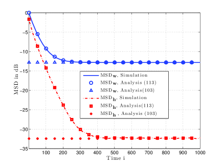
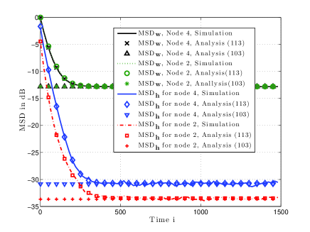
Refer to caption
(a) The network MSD.
Refer to caption
(b) The MSD at some individual nodes.
Figure 2: The network MSD learning curve for N=4𝑁4N=4.

Two important points in Fig. 2 need to be highlighted. First, note from the top plot that the network MSD for 𝒘~k,isubscript~𝒘𝑘𝑖{\tilde{\boldsymbol{w}}}_{k,i} is larger than that for 𝒉~k,isubscript~𝒉𝑘𝑖{\tilde{\boldsymbol{h}}}_{k,i}. This is because

\use@mathgroup\M@U\symAMSbE𝒉~k,i2=\use@mathgroup\M@U\symAMSbE𝒘~k,iBkTBk2\use@mathgroup\M@U\symAMSb𝐸superscriptnormsubscript~𝒉𝑘𝑖2\use@mathgroup\M@U\symAMSb𝐸subscriptsuperscriptnormsubscript~𝒘𝑘𝑖2superscriptsubscript𝐵𝑘𝑇subscript𝐵𝑘{\use@mathgroup\M@U\symAMSb{E}}\|\tilde{\boldsymbol{h}}_{k,i}\|^{2}={\use@mathgroup\M@U\symAMSb{E}}\|\tilde{\boldsymbol{w}}_{k,i}\|^{2}_{B_{k}^{T}B_{k}} (120)

so that the MSD of 𝒉~k,isubscript~𝒉𝑘𝑖{\tilde{\boldsymbol{h}}}_{k,i} is a weighted version of the MSD of 𝒘~k,isubscript~𝒘𝑘𝑖{\tilde{\boldsymbol{w}}}_{k,i}. In this experiment, the weighting leads to a lower estimation error. Second, note from the bottom plot that while the MSD values of 𝒘~k,isubscript~𝒘𝑘𝑖\tilde{\boldsymbol{w}}_{k,i} are largely independent of the node index, the same is not true for the MSD values of 𝒉~k,isubscript~𝒉𝑘𝑖\tilde{\boldsymbol{h}}_{k,i}. In previous studies on diffusion LMS strategies, it has been shown that, for strongly-connected networks, the network nodes approach a uniform MSD performance level [36]. The result in Fig. 2(b) supports this conclusion where it is seen that the MSD of 𝒘~k,isubscript~𝒘𝑘𝑖{\tilde{\boldsymbol{w}}}_{k,i} for nodes 2 and 4 converge to the same MSD level. However, note that the MSD of 𝒉~k,isubscript~𝒉𝑘𝑖{\tilde{\boldsymbol{h}}}_{k,i} is different for nodes 2 and 4. This difference in behavior is due to the difference in weighting across nodes from (120).

V-B Comparison with Centralized Solution

We next compare the performance of the diffusion strategy (39)-(42) with the centralized solution (34)–(35). We consider a network with N=10𝑁10N=10 nodes with the topology illustrated by Fig. 1. In this experiment, we set μk=0.02subscript𝜇𝑘0.02\mu_{k}=0.02 for all k𝑘k, while the other network parameters are obtained following the same construction described for Fig. 2. As the results in Fig. 3 indicate, the diffusion and centralized LMS solutions tend to the same MSD performance level in the w𝑤w domain. This conclusion is consistent with prior studies on the performance of diffusion strategies in the full-rank case over strongly-connected networks [36]. However, discrepancies in performance are seen between the distributed and centralized implementations in the hh domain, and the discrepancy tends to become larger for larger values of N𝑁N. This is because, in moving from the w𝑤w domain to the hh domain, the inherent aggregation of information that is performed by the centralized solution leads to enhanced estimates for the hkosuperscriptsubscript𝑘𝑜h_{k}^{o} variables. For example, if the estimates 𝒘k,isubscript𝒘𝑘𝑖\boldsymbol{w}_{k,i} which are generated by the distributed solution are averaged prior to computing the 𝒉k,isubscript𝒉𝑘𝑖\boldsymbol{h}_{k,i}, then it can be observed that the MSD values of 𝒉~k,isubscript~𝒉𝑘𝑖{\tilde{\boldsymbol{h}}}_{k,i} for both the centralized and the distributed solution will be similar.
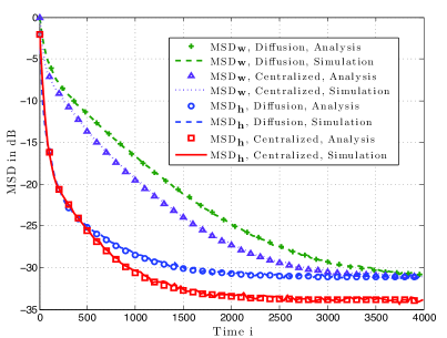
Refer to caption
(a) Nb=5subscript𝑁𝑏5N_{b}=5.
Refer to caption
(b) Nb=10subscript𝑁𝑏10N_{b}=10.
Figure 3: The network MSD learning curve for N=10𝑁10N=10.

In these experiments, we also observe that if we increase the number of basis functions, Nbsubscript𝑁𝑏N_{b}, then both the centralized and diffusion algorithms will converge faster but their steady-state MSD performance will degrade. Therefore, in choosing the number of basis functions, Nbsubscript𝑁𝑏N_{b}, there is a trade off between convergence speed and MSD performance.

V-C Example: Two-Dimensional Process Estimation

In this example, we consider a two-dimensional network with 13×13131313\times 13 nodes that are equally spaced over the unit square (x,y)[0,1]×[0,1]𝑥𝑦0101(x,y)\in[0,1]\times[0,1] with Δx=Δy=1/12Δ𝑥Δ𝑦112\Delta x=\Delta y=1/12 (see Fig. 4(a)). This network monitors a physical process f(x,y)𝑓𝑥𝑦f(x,y) described by the Poisson PDE:

2f(x,y)x2+2f(x,y)y2=h(x,y)superscript2𝑓𝑥𝑦superscript𝑥2superscript2𝑓𝑥𝑦superscript𝑦2𝑥𝑦\displaystyle\frac{\partial^{2}f(x,y)}{\partial x^{2}}+\frac{\partial^{2}f(x,y)}{\partial y^{2}}=h(x,y) (121)

where h(x,y):[0, 1]2\use@mathgroup\M@U\symAMSbR:𝑥𝑦superscript012\use@mathgroup\M@U\symAMSb𝑅h(x,y):[0,\,1]^{2}\rightarrow\use@mathgroup\M@U\symAMSb{R} is an unknown input function. The PDE satisfies the following boundary conditions:

f(x,0)=f(0,y)=f(x,1)=f(1,y)=0𝑓𝑥0𝑓0𝑦𝑓𝑥1𝑓1𝑦0\displaystyle f(x,0)=f(0,y)=f(x,1)=f(1,y)=0

For this problem, the objective is to estimate h(x,y)𝑥𝑦h(x,y), given noisy measurements collected by N=Nx×Ny=11×11𝑁subscript𝑁𝑥subscript𝑁𝑦1111N=N_{x}\times N_{y}=11\times 11 nodes corresponding to the interior points of the network. To discretize the PDE, we employ the finite difference method (FDM) with uniform spacing of ΔxΔ𝑥\Delta x and ΔyΔ𝑦\Delta y. We define xk1k1Δxsubscript𝑥subscript𝑘1subscript𝑘1Δ𝑥x_{k_{1}}\triangleq k_{1}\Delta x,  yk2k2Δysubscript𝑦subscript𝑘2subscript𝑘2Δ𝑦y_{k_{2}}\triangleq k_{2}\Delta y and introduce the sampled values fk1,k2f(xk1,yk2)subscript𝑓subscript𝑘1subscript𝑘2𝑓subscript𝑥subscript𝑘1subscript𝑦subscript𝑘2{f}_{k_{1},k_{2}}\triangleq f(x_{k_{1}},y_{k_{2}}) and hk1,k2oh(xk1,yk2)subscriptsuperscript𝑜subscript𝑘1subscript𝑘2subscript𝑥subscript𝑘1subscript𝑦subscript𝑘2h^{o}_{k_{1},k_{2}}\triangleq h(x_{k_{1}},y_{k_{2}}). We use the central difference scheme [39] to approximate the second order partial derivatives:

2f(x,y,t)x21Δx2[fk1+1,k22fk1,k2+fk11,k2]superscript2𝑓𝑥𝑦𝑡superscript𝑥21Δsuperscript𝑥2delimited-[]subscript𝑓subscript𝑘11subscript𝑘22subscript𝑓subscript𝑘1subscript𝑘2subscript𝑓subscript𝑘11subscript𝑘2\displaystyle\frac{{\partial}^{2}f(x,y,t)}{\partial x^{2}}\approx\frac{1}{\Delta x^{2}}[f_{k_{1}+1,k_{2}}-2f_{k_{1},k_{2}}+f_{k_{1}-1,k_{2}}] (122)
2f(x,y,t)y21Δy2[fk1,k2+12fk1,k2+fk1,k21]superscript2𝑓𝑥𝑦𝑡superscript𝑦21Δsuperscript𝑦2delimited-[]subscript𝑓subscript𝑘1subscript𝑘212subscript𝑓subscript𝑘1subscript𝑘2subscript𝑓subscript𝑘1subscript𝑘21\displaystyle\frac{{\partial}^{2}f(x,y,t)}{\partial y^{2}}\approx\frac{1}{\Delta y^{2}}[f_{k_{1},k_{2}+1}-2f_{k_{1},k_{2}}+f_{k_{1},k_{2}-1}] (123)

This leads to the following discretized input function:

hk1,k2o=subscriptsuperscript𝑜subscript𝑘1subscript𝑘2absent\displaystyle h^{o}_{k_{1},k_{2}}= 1Δx2(fk1+1,k2+fk1,k2+1+fk11,k2\displaystyle\frac{1}{\Delta x^{2}}\big{(}f_{k_{1}+1,k_{2}}+f_{k_{1},k_{2}+1}+f_{k_{1}-1,k_{2}}
+fk1,k214fk1,k2)\displaystyle\qquad+f_{k_{1},k_{2}-1}-4f_{k_{1},k_{2}}\big{)} (124)

For this example, the unknown input process is

hk1,k2o=eκ((k14)2+(k24)2)5eκ((k18)2+(k28)2)+1subscriptsuperscript𝑜subscript𝑘1subscript𝑘2superscript𝑒𝜅superscriptsubscript𝑘142superscriptsubscript𝑘2425superscript𝑒𝜅superscriptsubscript𝑘182superscriptsubscript𝑘2821h^{o}_{k_{1},k_{2}}=e^{-\kappa\big{(}(k_{1}-4)^{2}+(k_{2}-4)^{2}\big{)}}-5e^{-\kappa\big{(}(k_{1}-8)^{2}+(k_{2}-8)^{2}\big{)}}+1 (125)

where κ=(Nx1)2/4𝜅superscriptsubscript𝑁𝑥124\kappa=(N_{x}-1)^{2}/4.

Refer to caption
(a) Network topology.
Refer to caption
(b) fk1,k2subscript𝑓subscript𝑘1subscript𝑘2f_{k_{1},k_{2}} over the space.
Figure 4: Spatial distribution of f(x,y)𝑓𝑥𝑦f(x,y) over the network grid {(xk1,yk2)}subscript𝑥subscript𝑘1subscript𝑦subscript𝑘2\{(x_{k_{1}},y_{k_{2}})\}.
Refer to caption
Figure 5: Spatial distribution of SNR over the network.

To obtain fk1,k2subscript𝑓subscript𝑘1subscript𝑘2f_{k_{1},k_{2}}, we solve (121) using the Jacobi over-relaxation method [45]. Figure 4(b) illustrates the values of fk1,k2subscript𝑓subscript𝑘1subscript𝑘2f_{k_{1},k_{2}} over the spatial domain. For the estimation of hk1,k2subscriptsubscript𝑘1subscript𝑘2h_{k_{1},k_{2}}, the given information are the noisy measurement samples 𝒛k1,k2(i)=fk1,k2+𝒏k1,k2(i)subscript𝒛subscript𝑘1subscript𝑘2𝑖subscript𝑓subscript𝑘1subscript𝑘2subscript𝒏subscript𝑘1subscript𝑘2𝑖\boldsymbol{z}_{k_{1},k_{2}}(i)=f_{k_{1},k_{2}}+{\boldsymbol{n}}_{k_{1},k_{2}}(i). In this relation, the noise process 𝒏k1,k2(i)subscript𝒏subscript𝑘1subscript𝑘2𝑖{\boldsymbol{n}}_{k_{1},k_{2}}(i) is zero mean, temporally white and independent over space. For this network, the two dimensional reference signal is the distorted version of hk1,k2osubscriptsuperscript𝑜subscript𝑘1subscript𝑘2h^{o}_{k_{1},k_{2}} which is represented by 𝒅k1,k2(i)subscript𝒅subscript𝑘1subscript𝑘2𝑖\boldsymbol{d}_{k_{1},k_{2}}(i). The reference signal is obtained from (124) with fk1,k2subscript𝑓subscript𝑘1subscript𝑘2f_{k_{1},k_{2}} replaced by their noisy measured samples 𝒛k1,k2(i)subscript𝒛subscript𝑘1subscript𝑘2𝑖\boldsymbol{z}_{k_{1},k_{2}}(i), i.e.,

𝒅k1,k2(i)=subscript𝒅subscript𝑘1subscript𝑘2𝑖absent\displaystyle\boldsymbol{d}_{k_{1},k_{2}}(i)= 1Δx2(𝒛k1+1,k2(i)+𝒛k1,k2+1(i)+𝒛k11,k2(i)\displaystyle\frac{1}{\Delta x^{2}}\Big{(}\boldsymbol{z}_{k_{1}+1,k_{2}}(i)+\boldsymbol{z}_{k_{1},k_{2}+1}(i)+\boldsymbol{z}_{k_{1}-1,k_{2}}(i)
+𝒛k1,k21(i)4𝒛k1,k2(i))\displaystyle\qquad+\boldsymbol{z}_{k_{1},k_{2}-1}(i)-4\boldsymbol{z}_{k_{1},k_{2}}(i)\Big{)} (126)

According to (126), the linear regression model for this problem takes the following form:

𝒅k1,k2(i)=subscript𝒅subscript𝑘1subscript𝑘2𝑖absent\displaystyle\boldsymbol{d}_{k_{1},k_{2}}(i)= 𝒖k1,k2(i)hk1,k2o+𝒗k1,k2(i)subscript𝒖subscript𝑘1subscript𝑘2𝑖subscriptsuperscript𝑜subscript𝑘1subscript𝑘2subscript𝒗subscript𝑘1subscript𝑘2𝑖\displaystyle\boldsymbol{u}_{k_{1},k_{2}}(i)h^{o}_{k_{1},k_{2}}+{\boldsymbol{v}}_{k_{1},k_{2}}(i) (127)

where 𝒖k1,k2(i)=1subscript𝒖subscript𝑘1subscript𝑘2𝑖1\boldsymbol{u}_{k_{1},k_{2}}(i)=1. Therefore, in this example, we are led to a linear model (127) with deterministic as opposed to random regression data. Although we only studied the case of random regression data in this article, this example is meant to illustrate that the diffusion strategy can still be applied to models involving deterministic data in a manner similar to [1, 54].

To represent hk1,k2osubscriptsuperscript𝑜subscript𝑘1subscript𝑘2h^{o}_{k_{1},k_{2}} as a space-invariant parameter vector, we use two-dimensional shifted Chebyshev basis functions [55]. Using this representation, hk1,k2osubscriptsuperscript𝑜subscript𝑘1subscript𝑘2h^{o}_{k_{1},k_{2}} can be expressed as:

hk1,k2o=n=1Nbwnopn,k1,k2subscriptsuperscript𝑜subscript𝑘1subscript𝑘2superscriptsubscript𝑛1subscript𝑁𝑏subscriptsuperscript𝑤𝑜𝑛subscript𝑝𝑛subscript𝑘1subscript𝑘2\displaystyle h^{o}_{k_{1},k_{2}}=\sum_{n=1}^{N_{b}}w^{o}_{n}\,p_{n,k_{1},k_{2}} (128)

where each element of the two-dimensional basis set is:

pn,k1,k2=bn1,k1bn2,k2subscript𝑝𝑛subscript𝑘1subscript𝑘2subscript𝑏subscript𝑛1subscript𝑘1subscript𝑏subscript𝑛2subscript𝑘2\displaystyle p_{n,k_{1},k_{2}}=b_{n_{1},k_{1}}b_{n_{2},k_{2}} (129)

where {bn1,k1}subscript𝑏subscript𝑛1subscript𝑘1\{b_{n_{1},k_{1}}\} and {bn2,k2}subscript𝑏subscript𝑛2subscript𝑘2\{b_{n_{2},k_{2}}\} are the one-dimensional shifted Chebyshev polynomials in the x𝑥x and y𝑦y directions, respectively–recall (21).

In the network, each interior node communicates with its four immediate neighbors. We use A1=Isubscript𝐴1𝐼A_{1}=I and compute C𝐶C and A2subscript𝐴2A_{2} by using the Metropolis and relative degree rules [35, 2, 6]. All nodes are initialized at zero and μk=0.01subscript𝜇𝑘0.01\mu_{k}=0.01 for all k𝑘k. The signal-to-noise ratio (SNR) of the network is uniformly distributed in the range [20,30]2030[20,30]dB and is shown in Fig. 5.

Figures 6(a) and 6(b) show three dimensional views of the true and estimated input process using the proposed diffusion LMS algorithm after 300030003000 iterations. Figure 7 illustrates the MSD of the estimated source, i.e., limi\use@mathgroup\M@U\symAMSbEhk1,k2o𝒉k1,k2(i)2subscript𝑖\use@mathgroup\M@U\symAMSb𝐸superscriptnormsubscriptsuperscript𝑜subscript𝑘1subscript𝑘2subscript𝒉subscript𝑘1subscript𝑘2𝑖2\lim_{i\rightarrow\infty}{\use@mathgroup\M@U\symAMSb{E}}\|h^{o}_{k_{1},k_{2}}-\boldsymbol{h}_{k_{1},k_{2}}(i)\|^{2}.

Refer to caption
(a) True parameters.
Refer to caption
(b) Estimated parameters.
Figure 6: True and estimated hk1,k2osubscriptsuperscript𝑜subscript𝑘1subscript𝑘2h^{o}_{k_{1},k_{2}} by diffusion LMS.
Refer to caption
Figure 7: Network steady-state MSD performance in dB.

VI Conclusion

By combining interpolation and distributed adaptive optimization, we proposed a diffusion LMS strategy for estimation and tracking of space-time varying parameters over networks. The proposed algorithm can find the space-varying parameters not only at the node locations but also at spaces where no measurement is collected. We showed that if the network experiences data with rank-deficient covariance matrices, the non-cooperative LMS algorithm will converge to different solutions at different nodes. In contrast, the diffusion LMS algorithm is able to alleviate the rank-deficiency problem through its use of combination matrices especially since, as shown by (72), ρ()ρ(I)𝜌𝜌𝐼\rho({\cal B})\leq\rho(I-{\cal M}{\cal R}), where I𝐼I-{\cal M}{\cal R} is the coefficient matrix that governs the dynamics of the non-cooperative solution. Nevertheless, if these mechanisms fail to mitigate the deleterious effect of the rank-deficient data, then the algorithm converges to a solution space where the error is bounded. We analyzed the performance of the algorithm in transient and steady-state regimes, and gave conditions under which the algorithm is stable in the mean and mean-square sense.

Appendix A Mean Error Convergence

Based on the rank of =diag{R1,,RN}diagsubscript𝑅1subscript𝑅𝑁{\cal R}=\mbox{\rm{diag}}\{R_{1},\cdots,R_{N}\}, we have two possible cases:

a) Rk>0k{1,,N}subscript𝑅𝑘0for-all𝑘1𝑁R_{k}>0\;\forall k\in\{1,\cdots,N\}: As (68) implies, \use@mathgroup\M@U\symAMSbE[𝒘~i]\use@mathgroup\M@U\symAMSb𝐸delimited-[]subscript~𝒘𝑖{\use@mathgroup\M@U\symAMSb{E}}[\tilde{\boldsymbol{w}}_{i}] converges to zero if ρ()<1𝜌1\rho({\cal B})<1. In [6], it was shown that when >00{\cal R}>0, choosing the step-sizes according to (73) guarantees ρ()<1𝜌1\rho({\cal B})<1.

b) k{1,,N}𝑘1𝑁\exists k\in\{1,\cdots,N\} for which Rksubscript𝑅𝑘R_{k} is rank-deficient: For this case, we first show that

i+1b,(IΛ)i+1b,subscriptnormsuperscript𝑖1𝑏subscriptnormsuperscript𝐼Λ𝑖1𝑏\big{\|}{\cal B}^{i+1}\big{\|}_{b,\infty}\leq\big{\|}\big{(}I-{\cal M}\Lambda)^{i+1}\big{\|}_{b,\infty} (130)

where b,\|\cdot\|_{b,\infty} denotes the block-maximum norm for block vectors with block entries of size MNb×1𝑀subscript𝑁𝑏1MN_{b}\times 1 and block matrices with blocks of size MNb×MNb𝑀subscript𝑁𝑏𝑀subscript𝑁𝑏MN_{b}\times MN_{b}. To this end, we note that for the left-stochastic matrices A1subscript𝐴1A_{1} and A2subscript𝐴2A_{2}, we have 𝒜1Tb,=𝒜2Tb,=1subscriptnormsuperscriptsubscript𝒜1𝑇𝑏subscriptnormsuperscriptsubscript𝒜2𝑇𝑏1\|{\cal A}_{1}^{T}\|_{b,\infty}=\|{\cal A}_{2}^{T}\|_{b,\infty}=1 [6], and use the sub-multiplicative property of the block maximum norm [46] to write:

i+1b,subscriptnormsuperscript𝑖1𝑏\displaystyle\big{\|}{\cal B}^{i+1}\big{\|}_{b,\infty} 𝒜2Tb,Ib,𝒜1Tb,×absentsubscriptnormsuperscriptsubscript𝒜2𝑇𝑏subscriptnorm𝐼𝑏subscriptnormsuperscriptsubscript𝒜1𝑇𝑏\displaystyle\leq\|{\cal A}_{2}^{T}\|_{b,\infty}\;\|I-{\cal M}{\cal R}\|_{b,\infty}\;\|{\cal A}_{1}^{T}\|_{b,\infty}\times\cdots
×𝒜2Tb,Ib,𝒜1Tb,absentsubscriptnormsuperscriptsubscript𝒜2𝑇𝑏subscriptnorm𝐼𝑏subscriptnormsuperscriptsubscript𝒜1𝑇𝑏\displaystyle\qquad\times\|{\cal A}_{2}^{T}\|_{b,\infty}\;\|I-{\cal M}{\cal R}\|_{b,\infty}\;\|{\cal A}_{1}^{T}\|_{b,\infty}
=Ib,i+1absentsubscriptsuperscriptnorm𝐼𝑖1𝑏\displaystyle=\big{\|}I-{\cal M}{\cal R}\big{\|}^{i+1}_{b,\infty} (131)

If we introduce the (block) eigendecomposition of {\cal R} (71) into (131) and consider the fact that the block-maximum norm is invariant under block-diagonal unitary matrix transformations [6, 47], then inequality (131) takes the form:

i+1b,subscriptnormsuperscript𝑖1𝑏\displaystyle\big{\|}{\cal B}^{i+1}\big{\|}_{b,\infty} IΛb,i+1absentsubscriptsuperscriptnorm𝐼Λ𝑖1𝑏\displaystyle\leq\big{\|}I-{\mathcal{M}}{\Lambda}\big{\|}^{i+1}_{b,\infty} (132)

Using the property Xb,=ρ(X)subscriptnorm𝑋𝑏𝜌𝑋\|X\|_{b,\infty}=\rho(X) for a block diagonal Hermitian matrix X𝑋X [6], we obtain:

(IΛ)i+1b,=subscriptnormsuperscript𝐼Λ𝑖1𝑏absent\displaystyle\big{\|}(I-{\cal M}{\Lambda})^{i+1}\big{\|}_{b,\infty}= ρ((IΛ)i+1)𝜌superscript𝐼Λ𝑖1\displaystyle\rho\Big{(}(I-{\cal M}\Lambda)^{i+1}\Big{)}
=\displaystyle= max1kN1nMNb|(1μkλk(n))i+1|subscript1𝑘𝑁1𝑛𝑀subscript𝑁𝑏superscript1subscript𝜇𝑘subscript𝜆𝑘𝑛𝑖1\displaystyle\max_{\begin{subarray}{c}1\leq k\leq N\\ 1\leq n\leq MN_{b}\end{subarray}}\Big{|}\big{(}1-\mu_{k}\lambda_{k}(n)\big{)}^{i+1}\Big{|}
=\displaystyle= (max1kN1nMNb|1μkλk(n)|)i+1superscriptsubscript1𝑘𝑁1𝑛𝑀subscript𝑁𝑏1subscript𝜇𝑘subscript𝜆𝑘𝑛𝑖1\displaystyle\Big{(}\max_{\begin{subarray}{c}1\leq k\leq N\\ 1\leq n\leq MN_{b}\end{subarray}}|1-\mu_{k}\lambda_{k}(n)|\Big{)}^{i+1}
=\displaystyle= (ρ(IΛ))i+1superscript𝜌𝐼Λ𝑖1\displaystyle\Big{(}\rho(I-{\cal M}{\Lambda})\Big{)}^{i+1}
=\displaystyle= IΛb,i+1subscriptsuperscriptnorm𝐼Λ𝑖1𝑏\displaystyle\big{\|}I-{\cal M}{\Lambda}\big{\|}^{i+1}_{b,\infty} (133)

Using (133) in (132), we arrive at (130). We now proceed to show the boundedness of the mean error for case (b). We iterate (68) to get:

\use@mathgroup\M@U\symAMSbE[𝒘~i]=i+1\use@mathgroup\M@U\symAMSbE[𝒘~1]\use@mathgroup\M@U\symAMSb𝐸delimited-[]subscript~𝒘𝑖superscript𝑖1\use@mathgroup\M@U\symAMSb𝐸delimited-[]subscript~𝒘1\displaystyle{\use@mathgroup\M@U\symAMSb{E}}[\tilde{\boldsymbol{w}}_{i}]={\cal B}^{i+1}{\use@mathgroup\M@U\symAMSb{E}}[\tilde{\boldsymbol{w}}_{-1}] (134)

Applying the block maximum norm to (134) and using inequality (130), we obtain:

limi\use@mathgroup\M@U\symAMSbE[𝒘~i]b,subscript𝑖subscriptnorm\use@mathgroup\M@U\symAMSb𝐸delimited-[]subscript~𝒘𝑖𝑏\displaystyle\lim_{i\rightarrow\infty}\big{\|}{\use@mathgroup\M@U\symAMSb{E}}[\tilde{\boldsymbol{w}}_{i}]\big{\|}_{b,\infty} limi(IΛ)i+1b,\use@mathgroup\M@U\symAMSbE[𝒘~1]b,absentsubscript𝑖subscriptnormsuperscript𝐼Λ𝑖1𝑏subscriptnorm\use@mathgroup\M@U\symAMSb𝐸delimited-[]subscript~𝒘1𝑏\displaystyle\leq\lim_{i\rightarrow\infty}\big{\|}(I-{\cal M}\Lambda)^{i+1}\big{\|}_{b,\infty}\;\big{\|}{\use@mathgroup\M@U\symAMSb{E}}[\tilde{\boldsymbol{w}}_{-1}]\big{\|}_{b,\infty} (135)

The value of limi(IΛ)i+1b,subscript𝑖subscriptnormsuperscript𝐼Λ𝑖1𝑏\lim_{i\rightarrow\infty}\|(I-{\mathcal{M}}{\Lambda})^{i+1}\|_{b,\infty} can be computed by evaluating the limits of its diagonal entries. Considering the step-sizes as in (73), the diagonal entries are computed as:

limi(1μkλk(n))i+1={1,ifλk(n)=00,otherwisesubscript𝑖superscript1subscript𝜇𝑘subscript𝜆𝑘𝑛𝑖1cases1ifsubscript𝜆𝑘𝑛00otherwise\lim_{i\rightarrow\infty}\big{(}1-\mu_{k}\lambda_{k}(n)\big{)}^{i+1}=\left\{\begin{array}[]{l l}1,&\text{if}\,\lambda_{k}(n)=0\\ 0,&\text{otherwise}\end{array}\right. (136)

Therefore, (135) reads as:

limi\use@mathgroup\M@U\symAMSbE[𝒘~i]b,subscript𝑖subscriptnorm\use@mathgroup\M@U\symAMSb𝐸delimited-[]subscript~𝒘𝑖𝑏\displaystyle\lim_{i\rightarrow\infty}\big{\|}{\use@mathgroup\M@U\symAMSb{E}}[{\tilde{\boldsymbol{w}}}_{i}]\big{\|}_{b,\infty} IInd(Λ)b,\use@mathgroup\M@U\symAMSbE[𝒘~1]b,absentsubscriptnorm𝐼IndΛ𝑏subscriptnorm\use@mathgroup\M@U\symAMSb𝐸delimited-[]subscript~𝒘1𝑏\displaystyle\leq\|I-{\rm{Ind}}(\Lambda)\|_{b,\infty}\;\big{\|}{\use@mathgroup\M@U\symAMSb{E}}[\tilde{\boldsymbol{w}}_{-1}]\big{\|}_{b,\infty} (137)

Appendix B Mean Behavior When (A1=A2=Isubscript𝐴1subscript𝐴2𝐼A_{1}=A_{2}=I)

Setting A1=A2=Isubscript𝐴1subscript𝐴2𝐼A_{1}=A_{2}=I in the diffusion recursions (39)-(41) and subtracting wosuperscript𝑤𝑜w^{o} from both sides of (40), we get:

𝒘~k,i=𝒘~k,i1μk𝒩kc,kBT𝒖,iT(𝒅(i)𝒖,iB𝒘k,i1)subscript~𝒘𝑘𝑖subscript~𝒘𝑘𝑖1subscript𝜇𝑘subscriptsubscript𝒩𝑘subscript𝑐𝑘subscriptsuperscript𝐵𝑇subscriptsuperscript𝒖𝑇𝑖subscript𝒅𝑖subscript𝒖𝑖subscript𝐵subscript𝒘𝑘𝑖1\tilde{\boldsymbol{w}}_{k,i}=\tilde{\boldsymbol{w}}_{k,i-1}-\mu_{k}\sum_{\ell\in{\cal N}_{k}}c_{\ell,k}B^{T}_{\ell}\boldsymbol{u}^{T}_{\ell,i}(\boldsymbol{d}_{\ell}(i)-\boldsymbol{u}_{\ell,i}B_{\ell}\boldsymbol{w}_{k,i-1}) (138)

Under Assumption 1 and using 𝒅(i)=𝒖,iBwo+𝒗(i)subscript𝒅𝑖subscript𝒖𝑖subscript𝐵superscript𝑤𝑜subscript𝒗𝑖\boldsymbol{d}_{\ell}(i)=\boldsymbol{u}_{\ell,i}B_{\ell}w^{o}+\boldsymbol{v}_{\ell}(i), we obtain:

\use@mathgroup\M@U\symAMSbE[𝒘~k,i]\use@mathgroup\M@U\symAMSb𝐸delimited-[]subscript~𝒘𝑘𝑖\displaystyle{\use@mathgroup\M@U\symAMSb{E}}[\tilde{\boldsymbol{w}}_{k,i}] =Qk[IμkΛk]QkT\use@mathgroup\M@U\symAMSbE[𝒘~k,i1]absentsubscript𝑄𝑘delimited-[]𝐼subscript𝜇𝑘subscriptΛ𝑘subscriptsuperscript𝑄𝑇𝑘\use@mathgroup\M@U\symAMSb𝐸delimited-[]subscript~𝒘𝑘𝑖1\displaystyle=Q_{k}[I-\mu_{k}\Lambda_{k}]Q^{T}_{k}\,{\use@mathgroup\M@U\symAMSb{E}}[\tilde{\boldsymbol{w}}_{k,i-1}] (139)

We define 𝒑k,iQkT𝒘~k,isubscript𝒑𝑘𝑖superscriptsubscript𝑄𝑘𝑇subscript~𝒘𝑘𝑖\boldsymbol{p}_{k,i}\triangleq{Q}_{k}^{T}\tilde{\boldsymbol{w}}_{k,i} and start from some initial condition to arrive at

\use@mathgroup\M@U\symAMSbE[𝒑k,i]=[IμkΛk]\use@mathgroup\M@U\symAMSbE[𝒑k,i1]=[IμkΛk]i+1\use@mathgroup\M@U\symAMSbE[𝒑k,1]\use@mathgroup\M@U\symAMSb𝐸delimited-[]subscript𝒑𝑘𝑖delimited-[]𝐼subscript𝜇𝑘subscriptΛ𝑘\use@mathgroup\M@U\symAMSb𝐸delimited-[]subscript𝒑𝑘𝑖1superscriptdelimited-[]𝐼subscript𝜇𝑘subscriptΛ𝑘𝑖1\use@mathgroup\M@U\symAMSb𝐸delimited-[]subscript𝒑𝑘1\displaystyle{\use@mathgroup\M@U\symAMSb{E}}[\boldsymbol{p}_{k,i}]=[I-\mu_{k}\Lambda_{k}]{\use@mathgroup\M@U\symAMSb{E}}[\boldsymbol{p}_{k,i-1}]=[I-\mu_{k}\Lambda_{k}]^{i+1}{\use@mathgroup\M@U\symAMSb{E}}[\boldsymbol{p}_{k,-1}]

If we choose the step-sizes according to (73) then we get:

limi\use@mathgroup\M@U\symAMSbE[𝒑k,i]=[IInd(Λk)]\use@mathgroup\M@U\symAMSbE[𝒑k,1]subscript𝑖\use@mathgroup\M@U\symAMSb𝐸delimited-[]subscript𝒑𝑘𝑖delimited-[]𝐼IndsubscriptΛ𝑘\use@mathgroup\M@U\symAMSb𝐸delimited-[]subscript𝒑𝑘1\displaystyle\lim_{i\rightarrow\infty}{\use@mathgroup\M@U\symAMSb{E}}[\boldsymbol{p}_{k,i}]=\big{[}I-{\rm{Ind}}(\Lambda_{k})\big{]}{\use@mathgroup\M@U\symAMSb{E}}[\boldsymbol{p}_{k,-1}] (140)

Equivalently, this can be written as:

limi\use@mathgroup\M@U\symAMSbE[𝒘~k,i]=Qk[IInd(Λk)]QkT\use@mathgroup\M@U\symAMSbE[𝒘~k,1]subscript𝑖\use@mathgroup\M@U\symAMSb𝐸delimited-[]subscript~𝒘𝑘𝑖subscript𝑄𝑘delimited-[]𝐼IndsubscriptΛ𝑘subscriptsuperscript𝑄𝑇𝑘\use@mathgroup\M@U\symAMSb𝐸delimited-[]subscript~𝒘𝑘1\displaystyle\lim_{i\rightarrow\infty}{\use@mathgroup\M@U\symAMSb{E}}[{\tilde{\boldsymbol{w}}}_{k,i}]=Q_{k}\big{[}I-{\rm{Ind}}(\Lambda_{k})\big{]}Q^{T}_{k}\,{\use@mathgroup\M@U\symAMSb{E}}[{\tilde{\boldsymbol{w}}}_{k,-1}] (141)

This result indicates that the mean error does not grow unbounded. Now from (75), we can verify that:

QkInd(Λk)QkTwo=Rkrksubscript𝑄𝑘IndsubscriptΛ𝑘superscriptsubscript𝑄𝑘𝑇superscript𝑤𝑜superscriptsubscript𝑅𝑘subscript𝑟𝑘Q_{k}{\rm{Ind}}(\Lambda_{k})Q_{k}^{T}w^{o}=R_{k}^{\dagger}r_{k} (142)

Then, upon substitution of 𝒘~k,i=wo𝒘k,isubscript~𝒘𝑘𝑖superscript𝑤𝑜subscript𝒘𝑘𝑖\tilde{\boldsymbol{w}}_{k,i}=w^{o}-\boldsymbol{w}_{k,i} into (141), we obtain:

limi\use@mathgroup\M@U\symAMSbE[𝒘k,i]subscript𝑖\use@mathgroup\M@U\symAMSb𝐸delimited-[]subscript𝒘𝑘𝑖\displaystyle\lim_{i\rightarrow\infty}{\use@mathgroup\M@U\symAMSb{E}}[\boldsymbol{w}_{k,i}] =QkInd(Λk)QkTwo+Qk[IInd(Λk)]QkT\use@mathgroup\M@U\symAMSbE[𝒘k,1]absentsubscript𝑄𝑘IndsubscriptΛ𝑘superscriptsubscript𝑄𝑘𝑇superscript𝑤𝑜subscript𝑄𝑘delimited-[]𝐼IndsubscriptΛ𝑘superscriptsubscript𝑄𝑘𝑇\use@mathgroup\M@U\symAMSb𝐸delimited-[]subscript𝒘𝑘1\displaystyle=\small Q_{k}{\rm{Ind}}(\Lambda_{k})Q_{k}^{T}w^{o}+Q_{k}[I-{\rm{Ind}}(\Lambda_{k})]Q_{k}^{T}{\use@mathgroup\M@U\symAMSb{E}}[\boldsymbol{w}_{k,-1}]\normalsize
=Rkrk+n=Lk+1MNbqk,nqk,nT\use@mathgroup\M@U\symAMSbE[𝒘k,1]absentsuperscriptsubscript𝑅𝑘subscript𝑟𝑘superscriptsubscript𝑛subscript𝐿𝑘1𝑀subscript𝑁𝑏subscript𝑞𝑘𝑛superscriptsubscript𝑞𝑘𝑛𝑇\use@mathgroup\M@U\symAMSb𝐸delimited-[]subscript𝒘𝑘1\displaystyle=R_{k}^{\dagger}r_{k}+\sum_{n=L_{k}+1}^{MN_{b}}q_{k,n}q_{k,n}^{T}{\use@mathgroup\M@U\symAMSb{E}}[\boldsymbol{w}_{k,-1}] (143)

Appendix C Proof of Lemma 2

From (87), we readily deduce that

limii+1\use@mathgroup\M@U\symAMSbE[𝒘1]=(𝒵2𝒵¯2)\use@mathgroup\M@U\symAMSbE[𝒘1]subscript𝑖superscript𝑖1\use@mathgroup\M@U\symAMSb𝐸delimited-[]subscript𝒘1subscript𝒵2subscript¯𝒵2\use@mathgroup\M@U\symAMSb𝐸delimited-[]subscript𝒘1\displaystyle\lim_{i\rightarrow\infty}{\cal B}^{i+1}{\use@mathgroup\M@U\symAMSb{E}}[\boldsymbol{w}_{-1}]=({\cal Z}_{2}{\bar{\cal Z}}_{2})\,{\use@mathgroup\M@U\symAMSb{E}}[\boldsymbol{w}_{-1}] (144)

On the other hand, from (86), we have

limij=0ij𝒜2Tr=limij=0i(𝒵1Jj𝒵¯1+𝒵2𝒵¯2)𝒜2Trsubscript𝑖superscriptsubscript𝑗0𝑖superscript𝑗subscriptsuperscript𝒜𝑇2𝑟subscript𝑖superscriptsubscript𝑗0𝑖subscript𝒵1superscript𝐽𝑗subscript¯𝒵1subscript𝒵2subscript¯𝒵2subscriptsuperscript𝒜𝑇2𝑟\lim_{i\rightarrow\infty}\sum_{j=0}^{i}{\cal B}^{j}{\cal A}^{T}_{2}{\cal M}r=\lim_{i\rightarrow\infty}\sum_{j=0}^{i}\big{(}{\cal Z}_{1}J^{j}\bar{\cal Z}_{1}+{\cal Z}_{2}\bar{\cal Z}_{2}\big{)}{\cal A}^{T}_{2}{\cal M}r (145)

Using (88), the term involving 𝒵¯2subscript¯𝒵2\bar{\cal Z}_{2} cancels out and the above reduces to

limij=0ij𝒜2Trsubscript𝑖superscriptsubscript𝑗0𝑖superscript𝑗subscriptsuperscript𝒜𝑇2𝑟\displaystyle\lim_{i\rightarrow\infty}\sum_{j=0}^{i}{\cal B}^{j}{\cal A}^{T}_{2}{\mathcal{M}}r =limij=0i(𝒵1Jj𝒵¯1)𝒜2Trabsentsubscript𝑖superscriptsubscript𝑗0𝑖subscript𝒵1superscript𝐽𝑗subscript¯𝒵1subscriptsuperscript𝒜𝑇2𝑟\displaystyle=\lim_{i\rightarrow\infty}\sum_{j=0}^{i}\big{(}{\cal Z}_{1}J^{j}{\bar{\cal Z}_{1}}\big{)}{\cal A}^{T}_{2}{\mathcal{M}}r
=𝒵1(IJ)1𝒵¯1𝒜2Trabsentsubscript𝒵1superscript𝐼𝐽1subscript¯𝒵1subscriptsuperscript𝒜𝑇2𝑟\displaystyle={\cal Z}_{1}(I-J)^{-1}{\bar{\cal Z}_{1}}{\cal A}^{T}_{2}{\mathcal{M}}r (146)

since ρ(J)<1𝜌𝐽1\rho(J)<1. We now verify that the matrix

X=𝒵1(IJ)1𝒵¯1superscript𝑋subscript𝒵1superscript𝐼𝐽1subscript¯𝒵1X^{-}={\cal Z}_{1}(I-J)^{-1}{\bar{\cal Z}_{1}} (147)

is a (reflexive) generalized inverse for the matrix X=(I)𝑋𝐼X=(I-{\cal B}). Recall that a (reflexive) generalized inverse for a matrix Y𝑌Y is any matrix Ysuperscript𝑌Y^{-} that satisfies the two conditions [56]:

YYY𝑌superscript𝑌𝑌\displaystyle YY^{-}Y =Yabsent𝑌\displaystyle=Y (148)
YYYsuperscript𝑌𝑌superscript𝑌\displaystyle Y^{-}YY^{-} =Yabsentsuperscript𝑌\displaystyle=Y^{-} (149)

To verify these conditions, we first note from 𝒵𝒵1=I𝒵superscript𝒵1𝐼{\cal Z}{\cal Z}^{-1}=I and 𝒵1𝒵=Isuperscript𝒵1𝒵𝐼{\cal Z}^{-1}{\cal Z}=I in (86) that the following relations hold:

𝒵1𝒵¯1+𝒵2𝒵¯2=Isubscript𝒵1subscript¯𝒵1subscript𝒵2subscript¯𝒵2𝐼\displaystyle{\cal Z}_{1}{\bar{\cal Z}}_{1}+{\cal Z}_{2}{\bar{\cal Z}}_{2}=I (150)
𝒵¯1𝒵2=0subscript¯𝒵1subscript𝒵20\displaystyle{\bar{\cal Z}}_{1}{\cal Z}_{2}=0 (151)
𝒵¯2𝒵1=0subscript¯𝒵2subscript𝒵10\displaystyle{\bar{\cal Z}}_{2}{\cal Z}_{1}=0 (152)
𝒵¯1𝒵1=Isubscript¯𝒵1subscript𝒵1𝐼\displaystyle{\bar{\cal Z}}_{1}{\cal Z}_{1}=I (153)
𝒵¯2𝒵2=Isubscript¯𝒵2subscript𝒵2𝐼\displaystyle{\bar{\cal Z}}_{2}{\cal Z}_{2}=I (154)

We further note that X𝑋X can be expressed as:

X=(I)=𝒵1(IJ)𝒵¯1𝑋𝐼subscript𝒵1𝐼𝐽subscript¯𝒵1X=(I-{\cal B})={\cal Z}_{1}(I-J){\bar{\cal Z}_{1}} (155)

It is then easy to verify that the matrices {X,X}𝑋superscript𝑋\{X,X^{-}\} satisfy conditions (148) and (149), as claimed. Therefore, (146) can be expressed as:

limij=0ij𝒜2Tr=(I)𝒜2Trsubscript𝑖superscriptsubscript𝑗0𝑖superscript𝑗subscriptsuperscript𝒜𝑇2𝑟superscript𝐼subscriptsuperscript𝒜𝑇2𝑟\lim_{i\rightarrow\infty}\sum_{j=0}^{i}{\cal B}^{j}{\cal A}^{T}_{2}{\mathcal{M}}r=(I-{\cal B})^{-}{\cal A}^{T}_{2}{\mathcal{M}}r (156)

Substituting (144) and (156) into (78) leads to (89).

Let us now verify that the right-hand side of (89) remains invariant under basis transformations for the Jordan factors {𝒵1,𝒵¯1,𝒵2,𝒵¯2}subscript𝒵1subscript¯𝒵1subscript𝒵2subscript¯𝒵2\{{\cal Z}_{1},\bar{\cal Z}_{1},{\cal Z}_{2},\bar{\cal Z}_{2}\}. To begin with, the Jordan decomposition (86) is not unique. Let us assume, however, that we fix the central term diag{J,I}diag𝐽𝐼\mbox{\rm diag}\{J,I\} to remain invariant and allow the Jordan factors {𝒵1,𝒵¯1,𝒵2,𝒵¯2}subscript𝒵1subscript¯𝒵1subscript𝒵2subscript¯𝒵2\{{\cal Z}_{1},\bar{\cal Z}_{1},{\cal Z}_{2},\bar{\cal Z}_{2}\} to vary. It follows from (86) that

𝒵¯2=𝒵¯2,𝒵2=𝒵2formulae-sequencesubscript¯𝒵2subscript¯𝒵2subscript𝒵2subscript𝒵2\bar{\cal Z}_{2}{\cal B}=\bar{\cal Z}_{2},\;\;\;\;{\cal B}{\cal Z}_{2}={\cal Z}_{2} (157)

so that the columns of 𝒵2subscript𝒵2{\cal Z}_{2} and the rows of 𝒵¯2subscript¯𝒵2\bar{\cal Z}_{2} correspond to right and left-eigenvectors of {\cal B}, respectively, associated with the eigenvalues with value one. If we replace 𝒵2subscript𝒵2{\cal Z}_{2} by any transformation of the form 𝒵2𝒳2subscript𝒵2subscript𝒳2{\cal Z}_{2}{\cal X}_{2}, where 𝒳2subscript𝒳2{\cal X}_{2} is invertible, then by (154), 𝒵¯2subscript¯𝒵2\bar{\cal Z}_{2} should be replaced by 𝒳21𝒵¯2superscriptsubscript𝒳21subscript¯𝒵2{\cal X}_{2}^{-1}\bar{\cal Z}_{2}. This conclusion can also be seen as follows. The new factor 𝒵𝒵{\cal Z} is given by

𝒵[𝒵1𝒵2𝒳2]=[𝒵1𝒵2][I00𝒳2]𝒵delimited-[]subscript𝒵1subscript𝒵2subscript𝒳2delimited-[]subscript𝒵1subscript𝒵2delimited-[]𝐼00subscript𝒳2{\cal Z}\triangleq\left[\begin{array}[]{cc}{\cal Z}_{1}&{\cal Z}_{2}{\cal X}_{2}\end{array}\right]=\left[\begin{array}[]{cc}{\cal Z}_{1}&{\cal Z}_{2}\end{array}\right]\left[\begin{array}[]{cc}I&0\\ 0&{\cal X}_{2}\end{array}\right] (158)

and, hence, the new 𝒵1superscript𝒵1{\cal Z}^{-1} becomes

𝒵1=[𝒵¯1𝒳21𝒵¯2]superscript𝒵1delimited-[]subscript¯𝒵1subscriptsuperscript𝒳12subscript¯𝒵2{\cal Z}^{-1}=\left[\begin{array}[]{c}\bar{\cal Z}_{1}\\ {\cal X}^{-1}_{2}\bar{\cal Z}_{2}\end{array}\right] (159)

which confirms that 𝒵¯2subscript¯𝒵2\bar{\cal Z}_{2} is replaced by 𝒳21𝒵¯2subscriptsuperscript𝒳12subscript¯𝒵2{\cal X}^{-1}_{2}\bar{\cal Z}_{2}. It follows that the product 𝒵2𝒵¯2subscript𝒵2subscript¯𝒵2{\cal Z}_{2}\bar{\cal Z}_{2} remains invariant under arbitrary invertible transformations 𝒳2subscript𝒳2{\cal X}_{2}. Moreover, from (86) we also have that

𝒵¯1=J𝒵¯1,𝒵1=𝒵1Jformulae-sequencesubscript¯𝒵1𝐽subscript¯𝒵1subscript𝒵1subscript𝒵1𝐽\bar{\cal Z}_{1}{\cal B}=J\bar{\cal Z}_{1},\;\;\;\;{\cal B}{\cal Z}_{1}={\cal Z}_{1}J (160)

Assume we replace 𝒵1subscript𝒵1{\cal Z}_{1} by any transformation of the form 𝒵1𝒳1subscript𝒵1subscript𝒳1{\cal Z}_{1}{\cal X}_{1}, where 𝒳1subscript𝒳1{\cal X}_{1} is invertible, then by (153), 𝒵¯1subscript¯𝒵1\bar{\cal Z}_{1} should be replaced by 𝒳11𝒵¯1superscriptsubscript𝒳11subscript¯𝒵1{\cal X}_{1}^{-1}\bar{\cal Z}_{1}. However, since we want to maintain J𝐽J invariant, then this implies that the transformation 𝒳1subscript𝒳1{\cal X}_{1} must also satisfy

𝒳11J𝒳1=Jsuperscriptsubscript𝒳11𝐽subscript𝒳1𝐽{\cal X}_{1}^{-1}J{\cal X}_{1}=J (161)

It follows that the product 𝒵1(IJ)1𝒵¯1subscript𝒵1superscript𝐼𝐽1subscript¯𝒵1{\cal Z}_{1}(I-J)^{-1}\bar{\cal Z}_{1} remains invariant under such invertible transformations 𝒳1subscript𝒳1{\cal X}_{1}, since

𝒵1(IJ)1𝒵¯1subscript𝒵1superscript𝐼𝐽1subscript¯𝒵1\displaystyle{\cal Z}_{1}(I-J)^{-1}\bar{\cal Z}_{1} =\displaystyle= 𝒵1𝒳1𝒳11(IJ)1𝒳1𝒳11𝒵¯1subscript𝒵1subscript𝒳1superscriptsubscript𝒳11superscript𝐼𝐽1subscript𝒳1superscriptsubscript𝒳11subscript¯𝒵1\displaystyle{\cal Z}_{1}{\cal X}_{1}{\cal X}_{1}^{-1}(I-J)^{-1}{\cal X}_{1}{\cal X}_{1}^{-1}\bar{\cal Z}_{1} (162)
=\displaystyle= 𝒵1𝒳1(I𝒳11J𝒳1)1𝒳11𝒵¯1subscript𝒵1subscript𝒳1superscript𝐼superscriptsubscript𝒳11𝐽subscript𝒳11superscriptsubscript𝒳11subscript¯𝒵1\displaystyle{\cal Z}_{1}{\cal X}_{1}(I-{\cal X}_{1}^{-1}J{\cal X}_{1})^{-1}{\cal X}_{1}^{-1}\bar{\cal Z}_{1}
=\displaystyle= 𝒵1𝒳1(IJ)1𝒳11𝒵¯1subscript𝒵1subscript𝒳1superscript𝐼𝐽1superscriptsubscript𝒳11subscript¯𝒵1\displaystyle{\cal Z}_{1}{\cal X}_{1}(I-J)^{-1}{\cal X}_{1}^{-1}\bar{\cal Z}_{1}

Appendix D PROOF OF LEMMA 3

We first establish that 𝒵¯2𝒴subscript¯𝒵2𝒴\bar{\cal Z}_{2}{\cal Y} and 𝒴𝒵¯2T𝒴subscriptsuperscript¯𝒵𝑇2{\cal Y}\bar{\cal Z}^{T}_{2} are both equal to zero. Indeed, we start by replacing r𝑟r in (88) by its expression from (61) and (63) as r=𝒞Tcol{r¯du,1,,r¯du,N}𝑟superscript𝒞𝑇colsubscript¯𝑟𝑑𝑢1subscript¯𝑟𝑑𝑢𝑁r={\cal C}^{T}\mbox{\rm{col}}\{\bar{r}_{du,1},\cdots,\bar{r}_{du,N}\} that leads to:

𝒵¯2𝒜2T𝒞Tcol{r¯du,1,,r¯du,N}=0subscript¯𝒵2superscriptsubscript𝒜2𝑇superscript𝒞𝑇colsubscript¯𝑟𝑑𝑢1subscript¯𝑟𝑑𝑢𝑁0\bar{\cal Z}_{2}{\cal A}_{2}^{T}{\cal M}{\cal C}^{T}\mbox{\rm{col}}\{\bar{r}_{du,1},\cdots,\bar{r}_{du,N}\}=0 (163)

By further replacing r¯du,ksubscript¯𝑟𝑑𝑢𝑘\bar{r}_{du,k} by their values from (32), we obtain:

𝒵¯2𝒜2T𝒞Tdiag{B1T,,BNT}col{rdu,1,,rdu,N}=0subscript¯𝒵2superscriptsubscript𝒜2𝑇superscript𝒞𝑇diagsuperscriptsubscript𝐵1𝑇superscriptsubscript𝐵𝑁𝑇colsubscript𝑟𝑑𝑢1subscript𝑟𝑑𝑢𝑁0\bar{\cal Z}_{2}{\cal A}_{2}^{T}{\cal M}{\cal C}^{T}\mbox{\rm{diag}}\{B_{1}^{T},\cdots,B_{N}^{T}\}\mbox{\rm{col}}\{r_{du,1},\cdots,r_{du,N}\}=0 (164)

This relation must hold regardless of the cross-correlation vectors {rdu,k}subscript𝑟𝑑𝑢𝑘\{r_{du,k}\}. Therefore,

𝒵¯2𝒜2T𝒞Tdiag{B1T,,BNT}=0subscript¯𝒵2superscriptsubscript𝒜2𝑇superscript𝒞𝑇diagsuperscriptsubscript𝐵1𝑇superscriptsubscript𝐵𝑁𝑇0\bar{\cal Z}_{2}{\cal A}_{2}^{T}{\cal M}{\cal C}^{T}\mbox{\rm{diag}}\{B_{1}^{T},\cdots,B_{N}^{T}\}=0 (165)

We now define

𝒱=diag{σv,12IMNb,,σv,N2IMNb}𝒱diagsubscriptsuperscript𝜎2𝑣1subscript𝐼𝑀subscript𝑁𝑏subscriptsuperscript𝜎2𝑣𝑁subscript𝐼𝑀subscript𝑁𝑏{\cal V}=\mbox{\rm{diag}}\{\sigma^{2}_{v,1}I_{MN_{b}},\cdots,\sigma^{2}_{v,N}I_{MN_{b}}\} (166)

and rewrite expression (100) as

𝒴𝒴\displaystyle{\cal Y} =𝒜2T𝒞Tdiag{B1T,,BNT}diag{Ru,1,,Ru,N}absentsubscriptsuperscript𝒜𝑇2superscript𝒞𝑇diagsuperscriptsubscript𝐵1𝑇superscriptsubscript𝐵𝑁𝑇diagsubscript𝑅𝑢1subscript𝑅𝑢𝑁\displaystyle={\cal A}^{T}_{2}{\cal M}{\cal C}^{T}\mbox{\rm{diag}}\{B_{1}^{T},\cdots,B_{N}^{T}\}\mbox{\rm{diag}}\{R_{u,1},\cdots,R_{u,N}\}
×diag{B1,,BN}𝒱𝒞𝒜2absentdiagsubscript𝐵1subscript𝐵𝑁𝒱𝒞subscript𝒜2\displaystyle\qquad\times\mbox{\rm{diag}}\{B_{1},\cdots,B_{N}\}\,{\cal V}\,{\cal C}{\cal M}{\cal A}_{2} (167)

Multiplying this from the left by 𝒵¯2subscript¯𝒵2\bar{\cal Z}_{2} and comparing the result with (165), we conclude that

𝒵¯2𝒴=0subscript¯𝒵2𝒴0\bar{\cal Z}_{2}{\cal Y}=0 (168)

Noting that 𝒴𝒴{\cal Y} is symmetric, we then obtain:

𝒴𝒵¯2T=0𝒴subscriptsuperscript¯𝒵𝑇20{\cal Y}\bar{\cal Z}^{T}_{2}=0 (169)

Returning to recursion (102), we note first from (86) that {\cal B} can be rewritten as

=𝒵1J𝒵¯1+𝒵2𝒵¯2subscript𝒵1𝐽subscript¯𝒵1subscript𝒵2subscript¯𝒵2{\cal B}={\cal Z}_{1}J{\bar{\cal Z}_{1}}+{\cal Z}_{2}{\bar{\cal Z}}_{2} (170)

Since {\cal B} is power convergent, the first term on the right hand side of (102) converges to

limi\use@mathgroup\M@U\symAMSbE𝒘~1conditionalsubscript𝑖\use@mathgroup\M@U\symAMSb𝐸subscript~𝒘1\displaystyle\lim_{i\rightarrow\infty}{\use@mathgroup\M@U\symAMSb{E}}\|\tilde{\boldsymbol{w}}_{-1} (T)i+1Σi+12=\use@mathgroup\M@U\symAMSbE𝒘~1(𝒵2𝒵¯2)TΣ𝒵2𝒵¯22\displaystyle\|^{2}_{({\cal B}^{T})^{i+1}\Sigma{\cal B}^{i+1}}={\use@mathgroup\M@U\symAMSb{E}}\|{\tilde{\boldsymbol{w}}}_{-1}\|^{2}_{({\cal Z}_{2}\bar{\cal Z}_{2})^{T}\Sigma{\cal Z}_{2}\bar{\cal Z}_{2}} (171)

Substituting (170) into the second term on the right hand side of (102) and using (168) and (169), we arrive at

limij=0iTr((T)jΣj𝒴)=subscript𝑖superscriptsubscript𝑗0𝑖Trsuperscriptsuperscript𝑇𝑗Σsuperscript𝑗𝒴absent\displaystyle\lim_{i\rightarrow\infty}\sum_{j=0}^{i}{\rm{Tr}}\Big{(}({\cal B}^{T})^{j}\Sigma{\cal B}^{j}{\cal Y}\Big{)}= Tr(limij=0i(𝒵1Jj𝒵¯1)T\displaystyle{\rm{Tr}}\Big{(}\lim_{i\rightarrow\infty}\sum_{j=0}^{i}({\cal Z}_{1}J^{j}{\bar{\cal Z}_{1}})^{T}
×Σ(𝒵1Jj𝒵¯1)𝒴)\displaystyle\times\Sigma({\cal Z}_{1}J^{j}{\bar{\cal Z}_{1}}){\cal Y}\Big{)} (172)

If matrices X1subscript𝑋1X_{1}, X2subscript𝑋2X_{2} and ΣΣ\Sigma are of compatible dimensions, then the following relations hold[6]:

Tr(X1X2)=(vec(X2T))Tvec(X1)Trsubscript𝑋1subscript𝑋2superscriptvecsuperscriptsubscript𝑋2𝑇𝑇vecsubscript𝑋1\displaystyle{\rm{Tr}}(X_{1}X_{2})=\big{(}{\rm{vec}}(X_{2}^{T})\big{)}^{T}{\rm{vec}}(X_{1}) (173)
vec(X1ΣX2)=(X2TX1)vec(Σ)vecsubscript𝑋1Σsubscript𝑋2tensor-productsuperscriptsubscript𝑋2𝑇subscript𝑋1vecΣ\displaystyle{\rm{vec}}(X_{1}\Sigma X_{2})=(X_{2}^{T}\otimes X_{1}){\rm{vec}}(\Sigma) (174)

Using these relations in (172), we obtain

Tr(\displaystyle{\rm{Tr}}\Big{(} limij=0i(T)jΣj𝒴)=(vec(𝒴T))T\displaystyle\lim_{i\rightarrow\infty}\sum_{j=0}^{i}({\cal B}^{T})^{j}\Sigma{\cal B}^{j}{\cal Y}\Big{)}=\Big{(}{\rm{vec}}({\cal Y}^{T})\Big{)}^{T}
×(limij=0i(𝒵1Jj𝒵¯1)T(𝒵1Jj𝒵¯1)T)vec(Σ)absentsubscript𝑖superscriptsubscript𝑗0𝑖tensor-productsuperscriptsubscript𝒵1superscript𝐽𝑗subscript¯𝒵1𝑇superscriptsubscript𝒵1superscript𝐽𝑗subscript¯𝒵1𝑇vecΣ\displaystyle\times\Big{(}\lim_{i\rightarrow\infty}\sum_{j=0}^{i}({\cal Z}_{1}J^{j}{\bar{\cal Z}_{1}})^{T}\otimes({\cal Z}_{1}J^{j}{\bar{\cal Z}_{1}})^{T}\Big{)}{\rm{vec}}(\Sigma) (175)

This is equivalent to:

Tr(\displaystyle{\rm{Tr}}\Big{(} j=0(T)jΣj𝒴)=(vec(𝒴))T(j=0j)vec(Σ)\displaystyle\sum_{j=0}^{\infty}({\cal B}^{T})^{j}\Sigma{\cal B}^{j}{\cal Y}\Big{)}=\big{(}{\rm{vec}}({\cal Y})\big{)}^{T}\Big{(}\sum_{j=0}^{\infty}{\cal F}^{j}\Big{)}{\rm{vec}}(\Sigma) (176)

where

=((𝒵1𝒵1)(JJ)(𝒵¯1𝒵¯1))Tsuperscripttensor-productsubscript𝒵1subscript𝒵1tensor-product𝐽𝐽tensor-productsubscript¯𝒵1subscript¯𝒵1𝑇{\cal F}=\Big{(}({\cal Z}_{1}\otimes{\cal Z}_{1})(J\otimes J)({\bar{\cal Z}_{1}}\otimes{\bar{\cal Z}_{1}})\Big{)}^{T} (177)

Since ρ(JJ)<1𝜌tensor-product𝐽𝐽1\rho(J\otimes J)<1, the series converges and we obtain:

Tr(limi\displaystyle{\rm{Tr}}\Big{(}\lim_{i\rightarrow\infty} j=0i(T)jΣj𝒴)=(vec(𝒴))T(I)1vec(Σ)\displaystyle\sum_{j=0}^{i}({\cal B}^{T})^{j}\Sigma{\cal B}^{j}{\cal Y}\Big{)}=\Big{(}{\rm{vec}}({\cal Y})\Big{)}^{T}(I-{\cal F})^{-1}{\rm{vec}}(\Sigma) (178)

Upon substitution of (171) and (178) into (102), we arrive at (104).

References

  • [1] F. S. Cattivelli, C. G. Lopes, and A. H. Sayed, “Diffusion recursive least-squares for distributed estimation over adaptive networks,” IEEE Trans. on Signal Processing, vol. 56, no. 5, pp. 1865–1877, May 2008.
  • [2] F. S. Cattivelli and A. H. Sayed, “Diffusion LMS strategies for distributed estimation,” IEEE Trans. on Signal Processing, vol. 58, no. 3, pp. 1035–1048, Mar. 2010.
  • [3] J. Chen and A. H. Sayed, “Diffusion adaptation strategies for distributed optimization and learning over networks,” IEEE Trans. on Signal Processing, vol. 60, no. 8, pp. 4289–4305, Aug. 2012.
  • [4] S. Chouvardas, K. Slavakis, and S. Theodoridis, “Adaptive robust distributed learning in diffusion sensor networks,” IEEE Trans. on Signal Processing, vol. 59, no. 10, pp. 4692–4707, Oct. 2011.
  • [5] S. Y. Tu and A. H. Sayed, “Diffusion strategies outperform consensus strategies for distributed estimation over adaptive networks,” IEEE Trans. on Signal Processing, vol. 60, no. 12, pp. 6127–6234, Dec. 2012.
  • [6] A. H. Sayed, “Diffusion adaptation over networks,” in Academic Press Library in Signal Processing, R. Chellapa and S. Theodoridis, Eds., pp. 323–454, Academic Press, Elsevier, 2013. Also available as arXiv:1205.4220v2, May 2012.
  • [7] S. Y. Tu and A. H. Sayed, “Adaptive decision-making over complex networks,” in Proc. Asilomar Conference on Signals, Systems, and Computers, Pacific Grove, CA, Nov. 2012, pp. 525–530.
  • [8] P. D. Lorenzo, S. Barbarossa, and A. H. Sayed, “Decentralized resource assignment in cognitive networks based on swarming mechanisms over random graphs,” IEEE Trans. on Signal Processing, vol. 60, no. 7, pp. 3755–3769, July 2012.
  • [9] T. Lee and J. Seinfeld, “Estimation of two-phase petroleum reservoir properties by regularization,” J. of Computational Physics, vol. 69, no. 2, pp. 397–419, Feb. 1987.
  • [10] E. Holmes, M. Lewis, J. Banks, and R. Veit, “Partial differential equations in ecology: Spatial interactions and population dynamics,” Ecology, vol. 75, no. 1, pp. 17–29, Jan. 1994.
  • [11] M. Alpay and M. Shor, “Model-based solution techniques for the source localization problem,” IEEE Trans. on Control Systems Technology, vol. 8, no. 6, pp. 895–904, June 2000.
  • [12] N. Van Kampen, “Diffusion in inhomogeneous media,” J. of Physics and Chemistry of Solids, vol. 49, no. 1, pp. 673–677, June 1988.
  • [13] C. Chung and C. Kravaris, “Identification of spatially discontinuous parameters in second-order parabolic systems by piecewise regularization,” Inverse Problems, vol. 4, pp. 973–994, Feb. 1988.
  • [14] G. Richter, “Numerical identification of a spatially-varying diffusion coefficient,” Math. Comput., vol. 36, no. 154, pp. 375–386, Apr. 1981.
  • [15] V. Isakov and S. Kindermann, “Identification of the diffusion coefficient in a one-dimensional parabolic equation,” Inverse Problems, vol. 16, pp. 665–680, June 2000.
  • [16] M. Demetriou, “Process estimation and moving source detection in 2-D diffusion processes by scheduling of sensor networks,” in Proc. American Control Conf., New York City, July 2007, pp. 3432–3437.
  • [17] M. Demetriou and I. Hussein, “Estimation of spatially distributed processes using mobile spatially distributed sensor network,” SIAM Journal on Control and Optimization, vol. 48, no. 1, pp. 266–291, Feb. 2009.
  • [18] D. P. Bertsekas, “A new class of incremental gradient methods for least squares problems,” SIAM Journal on Opt., vol. 7, no. 4, pp. 913–926, Apr. 1997.
  • [19] A. Nedic and D. P. Bertsekas, “Incremental subgradient methods for nondifferentiable optimization,” SIAM J. Optim., vol. 12, no. 1, pp. 109–138, Jan. 2001.
  • [20] M. G. Rabbat and R. D. Nowak, “Quantized incremental algorithms for distributed optimization,” IEEE Journal on Selected Areas in Communications, vol. 23, no. 4, pp. 798–808, Apr. 2005.
  • [21] C. G. Lopes and A. H. Sayed, “Incremental adaptive strategies over distributed networks,” IEEE Trans. on Signal Processing, vol. 55, no. 8, pp. 4064–4077, Aug. 2007.
  • [22] L. Li, J. A. Chambers, C. G. Lopes, and A. H. Sayed, “Distributed estimation over an adaptive incremental network based on the affine projection algorithm,” IEEE Trans. on Signal Processing, vol. 58, no. 1, pp. 151–164, Jan. 2010.
  • [23] J. Tsitsiklis, D. Bertsekas, and M. Athans, “Distributed asynchronous deterministic and stochastic gradient optimization algorithms,” IEEE Trans. on Automatic Control, vol. 31, no. 9, pp. 803–812, Sept. 1986.
  • [24] L. Xiao, S. Boyd, and S. Lall, “A space-time diffusion scheme for peer-to-peer least-squares estimation,” in Proc. of the 5th Int. Conf. on Information Processing in Sensor networks (IPSN), Nashville, TN, April 2006, pp. 168–176.
  • [25] S. S. Stankovic, M. S. Stankovic, and D. M. Stipanovic, “Decentralized parameter estimation by consensus based stochastic approximation,” IEEE Trans. on Autom. Control, vol. 56, no. 3, pp. 531–543, Mar. 2011.
  • [26] P. Braca, S. Marano, and V. Matta, “Running consensus in wireless sensor networks,” in Proc. Int. Conf. on Information Fusion, Cologne, Germany, June 2008, pp. 1–6.
  • [27] S. Sardellitti, M. Giona, and S. Barbarossa, “Fast distributed average consensus algorithms based on advection-diffusion processes,” IEEE Trans. on Signal Processing, vol. 58, no. 2, pp. 826–842, Feb. 2010.
  • [28] T. Aysal, M. Yildiz, A. Sarwate, and A. Scaglione, “Broadcast gossip algorithms for consensus,” IEEE Trans. on Signal Processing, vol. 57, no. 7, pp. 2748–2761, July 2009.
  • [29] S. Boyd, A. Ghosh, B. Prabhakar, and D. Shah, “Randomized gossip algorithms,” IEEE Trans. on Information Theory, vol. 52, no. 6, pp. 2508–2530, June 2006.
  • [30] A. Dimakis, S. Kar, J. Moura, M. Rabbat, and A. Scaglione, “Gossip algorithms for distributed signal processing,” Proc. of the IEEE, vol. 98, no. 11, pp. 1847–1864, Nov. 2010.
  • [31] K. Srivastava and A. Nedic, “Distributed asynchronous constrained stochastic optimization,” IEEE Selected Topics on Signal Process., vol. 5, no. 4, pp. 772–790, Aug. 2011.
  • [32] S. Kar and J. Moura, “Convergence rate analysis of distributed gossip (linear parameter) estimation: Fundamental limits and tradeoffs,” IEEE Selected Topics on Signal Process., vol. 5, no. 4, pp. 674–690, Aug. 2011.
  • [33] P. Di Lorenzo and S. Barbarossa, “A bio-inspired swarming algorithm for decentralized access in cognitive radio,” IEEE Trans. on Signal Processing, vol. 59, no. 12, pp. 6160–6174, Dec. 2011.
  • [34] Y. Hu and A. Ribeiro, “Adaptive distributed algorithms for optimal random access channels,” IEEE Trans. on Wireless Communication, vol. 10, no. 8, pp. 2703 –2715, Aug. 2010.
  • [35] C. G. Lopes and A. H. Sayed, “Diffusion least-mean squares over adaptive networks: Formulation and performance analysis,” IEEE Trans. on Signal Processing, vol. 56, no. 7, pp. 3122–3136, July 2008.
  • [36] A. H. Sayed, S.-Y. Tu, J. Chen, X. Zhao, and Z. Towfic, “Diffusion strategies for adaptation and learning over networks,” IEEE Signal Process. Mag., vol. 30, pp. 155–171, May 2013.
  • [37] X. Zhao and A. H. Sayed, “Performance limits for distributed estimation over LMS adaptive networks,” IEEE Trans. on Signal Processing, vol. 60, no. 10, pp. 5107–5124, Oct. 2012.
  • [38] R. Mattheij, S. Rienstra, and J. ten Thije Boonkkamp, Partial Differential Equations: Modeling, Analysis, Computation.   Society for Industrial and Applied Mathematics, 2005.
  • [39] J. Thomas, Numerical Partial Differential Equations: Finite Difference Methods.   Springer Verlag, 1995.
  • [40] J. C. Mason and D. C. Handscomb, Chebyshev Polynomials.   Chapman & Hall/CRC, Boca Raton, FL, 2003.
  • [41] E. Isaaks and R. Srivastava, An Introduction to Applied Geostatistics.   Oxford University Press, NY, 1989.
  • [42] S.-J. Kim, E. Dall’Anese, and G. B. Giannakis, “Cooperative spectrum sensing for cognitive radios using kriged Kalman filtering,” IEEE Selected Topics in Signal Process., vol. 5, no. 1, pp. 24–36, Jan. 2011.
  • [43] N. A. Cressie, Statistics for Spatial Data.   Wiley, NY, 1993.
  • [44] S. Boyd, N. Parikh, E. Chu, B. Peleato, and J. Eckstein, Distributed Optimization and Statistical Learning via the Alternating Direction Method of Multipliers.   Now Publishers, 2011.
  • [45] D. P. Bertsekas and J. N. Tsitsiklis, Parallel and Distributed Computation.   Old Tappan, NJ (USA); Prentice Hall Inc., 1989.
  • [46] X. Zhao, S. Y. Tu, and A. H. Sayed, “Diffusion adaptation over networks under imperfect information exchange and non-stationary data,” IEEE Trans. on Signal Processing, vol. 60, no. 7, pp. 3460–3475, July 2012.
  • [47] N. Takahashi, I. Yamada, and A. H. Sayed, “Diffusion least-mean squares with adaptive combiners: Formulation and performance analysis,” IEEE Trans. on Signal Processing, vol. 58, no. 9, pp. 4795–4810, Sept. 2010.
  • [48] R. Abdolee and B. Champagne, “Diffusion LMS algorithms for sensor networks over non-ideal inter-sensor wireless channels,” in Proc. of Int. Conf. on Dist. Computing in Sensor Systems and Workshops, Barcelona, Spain, June 2011, pp. 1–6.
  • [49] D. McLernon, M. Lara, and A. Orozco-Lugo, “On the convergence of the LMS algorithm with a rank-deficient input autocorrelation matrix,” Signal Processing, vol. 89, pp. 2244–2250, Nov. 2009.
  • [50] C. D. Meyer, Matrix Analysis and Applied Linear Algebra.   SIAM, PA, 2000.
  • [51] R. A. Horn and C. R. Johnson, Matrix analysis.   Cambridge University press, 2003.
  • [52] A. H. Sayed, Adaptive Filters.   Wiley, NJ, 2008.
  • [53] T. Al-Naffouri and A. H. Sayed, “Transient analysis of data-normalized adaptive filters,” IEEE Trans. on Signal Processing, vol. 51, no. 3, pp. 639–652, Mar. 2003.
  • [54] F. Cattivelli and A. H. Sayed, “Distributed detection over adaptive networks using diffusion adaptation,” IEEE Trans. on Signal Processing, vol. 59, no. 5, pp. 1917–1932, May 2011.
  • [55] R. Mukundan, S. Ong, and P. A. Lee, “Image analysis by tchebichef moments,” IEEE Transactions on Image Processing, vol. 10, no. 9, pp. 1357–1364, Sept. 2001.
  • [56] A. Ben-Israel and T. N. Greville, Generalized Inverses: Theory and Applications.   Springer, 2003.
[Uncaptioned image] Reza Abdolee is currently a Ph.D. candidate at the Department of Electrical and Computer Engineering, McGill University, Montreal, Canada. In 2012, he was a research scholar at the Bell Labs, Alcatel-Lucent, Stuttgart, Germany. In 2011, he was a visiting Ph.D. student at the Department of Electrical Engineering, University of California, Los Angeles (UCLA). From 2006 to 2008, Mr. Abdolee worked as a staff engineer at the Wireless Communication Center, University of Technology, Malaysia (UTM), where he implemented a switch-beam smart antenna system for wireless network applications. His research interests include communication theory, statistical signal processing, optimization, and hardware design and integration. Mr. Abdolee was a recipient of several awards and scholarships, including, NSERC Postgraduate Scholarship, FQRNT Doctoral Research Scholarship, McGill Graduate Research Mobility Award, DAAD-RISE International Internship scholarship (Germany), FQRNT International Internship Scholarship, McGill Graduate Funding and Travel award, McGill International Doctoral Award, ReSMiQ International Doctoral Scholarship, Graduate Student Support Award (Concordia University), and International Tuition Fee Remission Award (Concordia University).
[Uncaptioned image] Benoit Champagne received the B.Ing. degree in Engineering Physics from the Ecole Polytechnique de Montr al in 1983, the M.Sc. degree in Physics from the Universit de Montr al in 1985, and the Ph.D. degree in Electrical Engineering from the University of Toronto in 1990. From 1990 to 1999, he was an Assistant and then Associate Professor at INRS-Telecommunications, Universit du Quebec, Montr al. In1999, he joined McGill University, Montreal, where he is now a Full Professor within the Department of Electrical and Computer Engineering. He also served as Associate Chairman of Graduate Studies in the Department from 2004 to 2007. His research focuses on the development and performance analysis of advanced algorithms for the processing of information bearing signals by digital means. His interests span many areas of statistical signal processing, including detection and estimation, sensor array processing, adaptive filtering, and applications thereof to broadband communications and speech processing, where he has published extensively. His research has been funded by the Natural Sciences and Engineering Research Council (NSERC) of Canada, the Fonds de Recherche sur la Nature et les Technologies from the Government of Quebec, Prompt Quebec, as well as some major industrial sponsors, including Nortel Networks, Bell Canada, InterDigital and Microsemi. He has been an Associate Editor for the IEEE Signal Processing Letters, the IEEE Trans. on Signal Processing and the EURASIP Journal on Applied Signal Processing. He has also served on the Technical Committees of several international conferences in the fields of communications and signal processing. He is currently a Senior Member of IEEE.
[Uncaptioned image] Ali H. Sayed is professor and former chairman of electrical engineering at the University of California, Los Angeles, where he directs the UCLA Adaptive Systems Laboratory. An author of over 430 scholarly publications and five books, his research involves several areas including adaptation and learning, information processing theories, statistical signal processing, network science, and biologically-inspired designs. His work has been recognized with several awards including the 2012 Technical Achievement Award from the IEEE Signal Processing Society, the 2005 Terman Award from the American Society for Engineering Education, a 2005 Distinguished Lecturer from the IEEE Signal Processing Society, the 2003 Kuwait Prize, and the 1996 IEEE Donald G. Fink Prize. He has also been awarded several paper awards from the IEEE Signal Processing Society (2002,2005,2012) and is a Fellow of both the IEEE and the American Association for the Advancement of Science (AAAS). He has been active in serving the Signal Processing community in various roles. Among other activities, he served as Editor-in-Chief of the IEEE Transactions on Signal Processing (2003-2005), Editor-in-Chief of the EURASIP J. on Advances in Signal Processing (2006-2007), General Chairman of ICASSP (Las, Vegas, 2008), and Vice-President of Publications of the IEEE Signal Processing Society (2009-2011). He also served as member of the Board of Governors (2007-2011), Awards Board (2005), Publications Board (2003-2005, 2009-2011), Conference Board (2007-2011), and Technical Directions Board (2008-2009) of the same Society and as General Chairman of the IEEE International Conference on Acoustics, Speech, and Signal Processing (ICASSP) 2008.