An asymptotic preserving scheme for kinetic models for chemotaxis phenomena

Abstract

In this paper, we propose a numerical scheme to solve the kinetic model for chemotaxis phenomena. Formally, this scheme is shown to be uniformly stable with respect to the small parameter, consistent with the fluid-diffusion limit (Keller-Segel model). Our approach is based on the micro-macro decomposition which leads to an equivalent formulation of the kinetic model that couples a kinetic equation with macroscopic ones. This method is validated with various test cases and compared to other standard methods.

keyword: Asymptotic preserving scheme; Kinetic theory; Micro-macro decomposition; Chemotaxis phenomena
MSC: 65M06, 35Q20, 82C22, 92B0

1 Introduction

Chemotaxis is a process by which cells change their movement by reacting to the presence of a chemical substance. Cells approach to chemically favorable environments and avoid unfavorable ones. In a simple description, where we only consider cells and a chemical substance (the chemo-attractant), a model for the space and time evolution of the density $n=n(t,x)$ of cells and the chemical concentration $S=S(t,x)$ at time $t$ and position $x$ has been introduced by Patlak [1] and Keller-Segel [2] reads:

$$\left\{\begin{array}[]{l}\partial_{t}n+\nabla_{x}\cdot\left(n\,\chi(S)\nabla_{x}{S}-D_{n}\nabla_{x}n\right)=0,\\ \partial_{t}S-D_{S}\Delta S=H(n,S),\end{array}\right.$$ (1)

where $\nabla_{x}$ denotes the gradient with respect to the spatial variable, while the positive defined constants $D_{S}$ and $D_{n}$ are the diffusivity of the chemo-attractant and of the cells, respectively, and $\chi$ is the chemotactic sensitivity.

In general the substance $S$ does not only diffuse in the substrate, but it can also be produced by the bacteria themselves. The role of t $H(n,S)$ consists in modeling the interaction between both quantities. A typical example is $H(n,S)=an-bS$, which describes the production of the chemo-attractant by the bacteria at a constant rate $a$ as well as chemical decay with relaxation time $\frac{1}{b}$. Since the bacterial movement is directed toward the higher concentrations of $S$, the coupling is attractive. A deep insight into the phenomenological derivation of Keller and Segel types models is given in the survey [3].

The qualitative analysis of Keller-Segel models has attracted several mathematicians and a variety of interesting results have been produced. The surveys [4] and [5] provide a detailed review and critical analysis of the qualitative properties of the solutions to problems related to the application to various biological contexts.

An alternative modeling approach has been introduced by the mesoscopic description which bridges the interaction of stochastic particle to macroscopic equations. This middle ground consists in describing the movement of cells by a “run & tumble” process [6, 7]. Cells move along a straight line in the running phase and make reorientation as a reaction to the surrounding chemicals during the tumbling phase. This is the typical behavior that has been observed in experiments. The resulting kinetic equation, with parabolic scaling, reads

$$\left\{\begin{array}[]{l}\varepsilon\partial_{t}f+v\cdot\nabla_{x}f=\frac{1}{\varepsilon}\mathcal{T}(S,f),\\ \partial_{t}S-D_{S}\Delta S=H(n,S),\\ f(0,x,v)=f_{0}(x,v),\end{array}\right.$$ (2)

where $f(t,x,v)$ denotes the density of cells, depending on time $t$, position $x\in\Omega\subset\mathbb{R}^{d}$ and velocity $v\in V\subset\mathbb{R}^{d}$. $\mathcal{T}$ is an operator, which models the change of direction of cells and $\varepsilon$ is a time scale which here refers to the turning frequency. The function $S(t,x)$ is the chemical concentration, where $n$ denotes the density of cells, and is given by

$${n(t,x)=\int_{V}f(t,x,v)dv}.$$

Starting with the kinetic equation (2), one can (at least formally) derive the macroscopic limit (1) as $\varepsilon\rightarrow 0$. Various asymptotic limits, including hyperbolic limits, have been investigated in [8, 9, 10, 11, 12].

The aim of this paper is the development of numerical schemes to solve the kinetic equation by methods that are uniformly stable along the transition from kinetic regime to the fluid regime. The main difficulty is due to the term $\frac{1}{\varepsilon}$ which becomes stiff when $\varepsilon$ is close to zero (macroscopic regime). In this case, solving the kinetic equation by a standard explicit numerical scheme requires the use of a time step of the order of $\varepsilon$, which leads to very expensive numerical computations for small $\varepsilon$. To avoid this difficulty, it is necessary to use an implicit or semi-implicit time discretization for the collision part. In fact, such numerical schemes should also have a correct asymptotic behavior, namely for small parameter $\varepsilon$, the schemes should degenerate into a good approximation of the asymptotics (Keller-Segel model) of the kinetic equation. This property is often called “asymptotic preserving”, and has been introduced in [13] for numerical schemes that are stable with respect to a small parameter $\varepsilon$ and degenerate into a consistent numerical scheme for the limit model when $\varepsilon\rightarrow 0$.

Considering that this paper deals with asymptotic preserving scheme (AP), one also has to mention that there are different approaches to construct such schemes for kinetic models in various contexts. We mention for instance approaches based on domain decompositions, separating the macroscopic (fluid) domain from the microscopic (kinetic) one (see [14, 15]). There are other kind of (AP) schemes for kinetic equations, which are based on the use of time relaxed techniques where the Boltzmann collision operator is discretized by a spectral or a Monte-Carlo method (see [16, 17, 18]). Various techniques have also been developed to design multiscale numerical methods which are based on splitting strategy [19, 20, 21, 22, 23], penalization procedure [24, 25, 26, 27] or micro-macro decomposition which first was used by Liu and Yu for theoretical study of the fluid limit of the Boltzmann equation [28]. It was then used to develop an AP scheme for different asymptotics (diffusion, fluid, high-field, …), see [29, 30, 31, 32, 33, 34, 35, 36].

In this paper, we extend a method of micro-macro decomposition in order to construct asymptotic preserving schemes (AP) for kinetic equations describing chemotaxis phenomena. Our strategy consists in rewriting the kinetic equation as a coupled system of kinetic part and macroscopic one, by using the micro-macro decomposition of the distribution function. Indeed, this function is decomposed into its corresponding equilibrium distribution plus the deviation. By using a classical projection technique, we obtain an evolution equation for the macroscopic parameters of the equilibrium coupled to a kinetic equation for the non-equilibrium part. Although our approach is rather general to apply to a very large class of collision operators, the numerical tests shown in our work were obtained with very simple model. The outline of the contents are the following. In Section 2, we present the kinetic model and its properties. The micro-macro decomposition, the corresponding formulation of the kinetic equation, and the macroscopic limit are presented in Section 3. Our numerical scheme is presented in Section 4. Finally, a numerical test is presented in Section 5.

2 The kinetic model

This section provides a description of the kinetic model in the first equation in (2), where the turning kernel $\mathcal{T}$ defines the probability density of the random velocity jump of cells from $v^{\prime}$ to $v$. To derive the Keller- Segel equation (1) as $\varepsilon\rightarrow 0$, one has to incorporate both $O(1)$ and $O(\varepsilon)$ scale into $\mathcal{T}$.

We suppose, as in [8, 11, 37, 38], the following perturbation of the turning operator:

$$\mathcal{T}(S,f)=\mathcal{T}_{0}(f)+\varepsilon\mathcal{T}_{1}(S)(f),$$ (3)

where $\mathcal{T}_{0}$, supposed independent of $S$, represents the dominant part of the turning kernel modeling the tumble process in the absence of chemical substance, while $\mathcal{T}_{1}(S)$ defines the perturbation due to chemical cues.

Let us now state the assumptions on the turning operators $\mathcal{T}_{0}$ and $\mathcal{T}_{1}(S)$ which are necessary to develop the perturbation approach:

$\bullet$ The operators $\mathcal{T}_{0}$ and $\mathcal{T}_{1}$ preserve the local mass:

$$\int_{V}\mathcal{T}_{0}(f)dv=\int_{V}\mathcal{T}_{1}(S,f)dv=0,\quad\text{for any}\quad S\geq 0.$$ (4)

$\bullet$ There exists a bounded velocity distribution $M(v)>0$, independent of $x$ and $t$, such that the flow produced by the equilibrium distribution $M$ vanishes, and $M$ is normalized:

$$\int_{V}vM(v)dv=0,\qquad\int_{V}M(v)dv=1.$$ (5)

$\bullet$ The detailed balance

$$T_{0}(v^{\prime},v)M(v)=T_{0}(v,v^{\prime})M(v^{\prime})$$ (6)

holds.

$\bullet$ The kernel $T_{0}(v,v^{\prime})$ is bounded, and there exists a constant $\sigma>0$ such that

$$T_{0}(v,v^{\prime})\geq\sigma M,\quad\forall(v,v^{\prime})\in V\times V,\quad x\in\mathbb{R}^{d},\quad t>0.$$ (7)

The most commonly used assumption on the turning operators $\mathcal{T}_{i}$ , $i=0,1$, is that they are both linear integral operators with respect to $f$ and read:

$$\mathcal{T}_{i}(S,f)=\int_{V}(T_{i}(S,v,v^{\prime})f(t,x,v^{\prime})-T_{i}(S,v^{\prime},v)f(t,x,v))dv^{\prime},$$ (8)

where the turning kernel $T_{1}(S,v,v^{\prime})$ describes the reorientation of cells, i.e. the random velocity changes from $v$ to $v^{\prime}$ and may depend on the chemo-attractant concentration and its derivatives.

Technical calculations (see [8, 39]), namely by integration over $v$, interchanging $v$ by $v^{\prime}$, and using (6), yields:

where

$$\Psi[M]=\frac{1}{2}\,\big{(}T_{0}(v,v^{\prime})M(v^{\prime})+T_{0}(v^{\prime},v)M(v)\big{)}.$$

In particular Eq.(9) shows that the operators $\mathcal{T}_{0}$, is a self-adjoint and the following equality:

$$-\int_{V}\mathcal{T}_{0}(h)\frac{h(v)}{M(v)}\,dv=\frac{1}{2}\int_{V}\int_{V}\Psi[M]\bigg{(}\frac{h(v)}{M(v)}-\frac{h(v^{\prime})}{M(v^{\prime})}\bigg{)}^{2}\,dv\,dv^{\prime}\geq 0$$ (10)

holds true.

Moreover, for $\int_{V}h(v)\,dv=0$, Eq.(10) and the estimate (7) yield:

$$-\int_{V}\mathcal{T}_{0}(h)\frac{h(v)}{M(v)}\,dv\geq\sigma\int_{V}\frac{h^{2}(v)}{M(v)}\,dv,$$ (11)

which shows that $\mathcal{T}_{0}$ is a Fredholm operator in the space $L^{2}(V,\frac{dv}{M(v)})$. Therefore, the following result defines the properties of the operator $\mathcal{T}_{0}$:

Lemma 1.

Suppose that Assumptions (5)-(7) hold. Then, the following properties of the operators $\mathcal{T}_{0}$ hold true:

• The operator $\mathcal{T}_{0}$ is self-adjoint in the space $\displaystyle{{L^{2}\left(V,\frac{dv}{M}\right)}}$.

• For $\displaystyle{f\in L^{2}\left(V,\frac{dv}{M}\right)}$, the equation $\mathcal{T}_{0}(g)=f$, has a unique solution $\displaystyle{g\in L^{2}\left(V,\frac{dv}{M}\right)}$, which satisfies $\displaystyle{\int_{V}g(v)\,dv=0}$ if and only if $\displaystyle{\int_{V}f(v)\,dv=0.}$

• The equation $\mathcal{T}_{0}(g)=v\,M(v)$, has a unique solution that we call $\theta(v)$.

• The kernel of $\mathcal{T}_{0}$ is $N(\mathcal{T}_{0})=vect(M(v))$.

3 micro-macro decomposition and macroscopic limit

3.1 The micro-macro decomposition

Let $(f,S)$ be a solution of (2). We decompose $f$ as follows:

$$f=M(v)n+\varepsilon g,$$

where $n$ is the density of cells. Then $\langle g\rangle=\int_{V}gdv=0$, and:

Let us now use a projection technique to separate the macroscopic and microscopic quantities $n(t,x)$ and $g(t,x,v)$. Moreover, let $P_{M}$, denote the orthogonal projection onto $N(\mathcal{T}_{0})$. Then

$$P_{M}(h)=\langle h\rangle M,\quad\mbox{for any}\quad h\in L^{2}(V,\frac{dv}{M(v)}),$$

so that one has the following:

Lemma 2.

One has the following properties for the projection $P_{M}$:

$$(I-P_{M})(Mn)=P_{M}(g)=0,$$

$$(I-P_{M})(vM\cdot\nabla_{x}n)=vM\cdot\nabla_{x}n,$$

$$(I-P_{M})(\mathcal{T}_{1}(S)(M(v)n)=\mathcal{T}_{1}(S)(M(v)n),$$

and

$$(I-P_{M})(\mathcal{T}_{1}(S)(g))=\mathcal{T}_{1}(S)(g)$$

.

Proof.

The first two equalities can be rapidly proved since $P_{M}(M)=M$, and $\langle g\rangle=0$, as the flux produced by $M$ is zero then

$$(I-P_{M})(vM\cdot\nabla_{x}n)=vM\cdot\nabla_{x}n.$$

In addition, using (4) yields $P_{M}(\mathcal{T}_{1}(S)(h))=0$ for any $h\in L^{2}$, so that the third and the fourth equality are completed. ∎

Taking the operator $I-P_{M}$ into the equation (12) and using Lemma 2 yields

Integrating (12) over $v$, yields

$$\frac{\partial n}{\partial t}+\langle v\cdot\nabla_{x}g\rangle=0.$$ (14)

So that the micro-macro formulation finally reads:

Equations (15) correspond to the micro-macro formulation of the kinetic equation (2) to be used to design our AP scheme. The following Proposition shows that this formulation is indeed equivalent to the kinetic equation (2).

Proposition 1.

1. Let $(f,S)$ be a solution of (2) with initial data $(f_{0},S_{0})$. Then $(n,g,S)$, where $n=\langle f\rangle$ and $g=\frac{1}{\varepsilon}(f-M(v)n)$ is a solution to a coupled system (15) with the associated initial data:

   $n(t=0)=n_{0}=\langle f_{0}\rangle$, $g(t=0)=g_{0}=\frac{1}{\varepsilon}(f_{0}-M(v)n_{0})$, and $S(t=0)=S_{0}.$

2. Conversely, if $(n,g,S)$ satisfies system (15) with initial data $(n_{0},g_{0},S_{0})$ such that $\langle g_{0}\rangle=0$ then $f=M(v)n+\varepsilon g$ is a solution to kinetic model (2) with initial data $f_{0}=M(v)n_{0}+\varepsilon g_{0}$, and we have $n=\langle f\rangle$, and $\langle g\rangle=0.$

Proof.

The proof of 1) is detailed above. For 2), consider $(n,g,S)$ solution of (15). We set $f=M(v)n+\varepsilon g$ and we show that $f$ is a solution of kinetic model (2). From (15), one has

$$\frac{\partial f}{\partial t}-M(v)\frac{\partial n}{\partial t}+\frac{1}{\varepsilon}vM\cdot\nabla_{x}n+v\cdot\nabla_{x}g-P_{M}(v\cdot\nabla_{x}g)=\frac{1}{\varepsilon^{2}}\mathcal{T}_{0}(f)+\frac{1}{\varepsilon}\mathcal{T}_{1}(S)(f).$$

Hence

$$\frac{\partial f}{\partial t}-M(v)\frac{\partial n}{\partial t}+\frac{1}{\varepsilon}v\cdot\nabla_{x}f-M(v)\langle v\cdot\nabla_{x}g\rangle=\frac{1}{\varepsilon^{2}}\mathcal{T}_{0}(f)+\frac{1}{\varepsilon}\mathcal{T}_{1}(S)(f).$$

Therefore using (14), one obtains (2). The property $\langle g\rangle=0$ is obtained by integrating (13) over $v$, using (4) and the property of the initial data. This completes the proof. ∎

3.2 The macroscopic limit

In this subsection, the formal derivation of the macroscopic model is developed starting from the meso-macro model (2). The macroscopic model has been derived mathematically in [39]. We will see that the formal derivation is really straightforward starting from (15) (compared to the equivalent formulation of (2)), since the micro-macro model is well suited to deal with the asymptotic model in the diffusion limit. Indeed for small $\varepsilon$, the first equation of (15) by using (4) and (5) yields

$$g=\mathcal{T}_{0}^{-1}(vM\cdot\nabla_{x}n)-\mathcal{T}_{0}^{-1}(\mathcal{T}_{1}(S)(M(v)n))+O(\varepsilon).$$ (16)

Inserting (16) into (14) yields the asymptotic model (coupled with the concentration equation for $S$):

Using iii) of Lemma 1, one has as $\mathcal{T}_{0}$ is a self adjoint operator in $L^{2}(\frac{dv}{M(v)})$ the following:

$$\left\langle v.\nabla_{x}(\mathcal{T}_{0}^{-1}(\mathcal{T}_{1}(S)(M(v)n))\right\rangle = \left\langle\mathcal{T}_{0}(\theta(v)).\frac{\nabla_{x}}{M(v)}(\mathcal{T}_{0}^{-1}(\mathcal{T}_{1}(S)(M(v)n))\right\rangle$$

$$= div_{x}\left\langle\frac{\theta(v)}{M(v)}n\mathcal{T}_{1}(S)(M(v))\right\rangle,$$

and consequently the macroscopic model (17) writes

$$\left\{\begin{array}[]{l}\frac{\partial n}{\partial t}+div_{x}\,(n\,\alpha(S)-D_{n}\nabla_{x}n)=O(\varepsilon),\\ {}\\ \frac{\partial S}{\partial t}-D_{S}\Delta S=H(n,S),\end{array}\right.$$ (18)

where $D_{n}$ and $\alpha(S)$ are given by

$$\qquad D_{n}=-\int_{V}v\otimes\theta(v)dv,\quad\alpha(S)=-\int_{V}\frac{\theta(v)}{M(v)}\mathcal{T}_{1}(S)(M)(v)dv.$$ (19)

Our approach appears to be quite general, while the Keller-Segel model can be derived. Let us consider probability kernels such that $T_{0}(v,v^{\prime})=\sigma M(v),\quad\sigma>0$. Consequently, the leading turning operators $\mathcal{T}_{0}$ become relaxation operators:

$$\mathcal{T}_{0}(g)=-\sigma\Big{(}g-\left\langle g\right\rangle M\Big{)}.$$ (20)

In particular, $\theta$ and the diffusion tensor $D_{n}$ are given by:

$$\theta(v)=-\frac{1}{\sigma}\,M(v),\quad D_{n}=\frac{1}{\sigma}\int_{V}v\otimes vM(v)dv.$$ (21)

In addition, $\alpha(S)$ is given by:

$$\alpha(S)=\frac{1}{\sigma}\int_{V}v\mathcal{T}_{1}[S](M(v))dv.$$ (22)

Then, together with the choice $T_{1}[S]=K_{S}(v,v^{\prime})\cdot\nabla_{x}S$, where $K_{S}(v,v^{\prime})$ is a vector valued function, yields $\mathcal{T}_{1}[S](M)=h(v,S)\cdot\nabla_{x}S$, where

$$h(v,S)=\int_{V}\Big{(}K_{S}(v,v^{\prime})M(v^{\prime})-K_{S}(v^{\prime},v)M(v)\Big{)}dv^{\prime}.$$

Finally, the function $\alpha(S)$ in (22) is given by $\alpha(S)=\chi(S)\cdot\nabla_{x}S$, where the chemotactic sensitivity $\chi(S)$ is given by the matrix

$$\chi(S)=\frac{1}{\sigma}\int_{V}v\otimes h(v,S)dv.$$ (23)

Therefore, the drift term $div_{x}(n\,\alpha(S))$ that appears in the macroscopic case stated by (17) becomes

$$div_{x}(n\,\alpha(S))=div_{x}\left(n\,\chi(S)\nabla_{x}{S}\right),$$

which gives a Keller-Segel type model (1):

$$\left\{\begin{array}[]{l}\partial_{t}n+div_{x}\,\left(n\,\chi(S)\cdot\nabla_{x}{S}-D_{n}\nabla_{x}n\right)=O(\varepsilon),\\ {}\\ \partial_{t}S-D_{S}\Delta S=H(n,S).\end{array}\right.$$ (24)

4 Numerical methods

Let us now consider Problem (2), subject to the following initial conditions: $f(0,x,v)=f_{0}(x,v)$ and $S(0,x)=S_{0}(x)$. It has been shown that problem (2) is equivalent to the following micro-macro formulation:

$$\left\{\begin{array}[]{l}\frac{\partial g}{\partial t}+\frac{1}{\varepsilon^{2}}vM\cdot\nabla_{x}n+\frac{1}{\varepsilon}(I-P_{M})(v\cdot\nabla_{x}g)=\frac{1}{\varepsilon^{2}}\mathcal{T}_{0}(g)\\ {}\\ \qquad\qquad\qquad+\frac{1}{\varepsilon^{2}}\mathcal{T}_{1}(S)(M(v)n)+\frac{1}{\varepsilon}\mathcal{T}_{1}(S)(g),\\ {}\\ \frac{\partial n}{\partial t}+\langle v\cdot\nabla_{x}g\rangle=0,\\ {}\\ \frac{\partial S}{\partial t}-D_{S}\Delta S=H(n,S),\end{array}\right.$$ (25)

subject to the following initial conditions:

The discretization of problem (25)-(26) is carried out for each independent variable (time, velocity and space).

4.1 Time discretization

The treatment of the time variable of problem (25)-(26) can be done by using varieties of methods such as finite difference and variational methods. Finite-differentiation of the derivative in time is the widely used approach.

The time interval $[0,T]$ is divided into $N$ times steps as follows: $t_{0}=0,\quad t_{k+1}=t_{k}+\Delta t,\quad 0\leq k<N,$ where $\Delta t=\frac{T}{N}$ is the time step. The approximation of $n(t,x)$ and $g(t,x,v)$ at the time step $t_{k}$ are denoted respectively by $n^{k}\approx n(t_{k},x)$ and $g^{k}\approx g(t_{k},x,v)$. Using an implicit scheme for the stiff term $\frac{1}{\varepsilon^{2}}\mathcal{T}_{0}(g)$ and an explicit for the other terms in the first equation in (25), one obtains :

$$\frac{g^{k+1}-g^{k}}{\Delta t} = -\frac{1}{\varepsilon^{2}}vM\cdot\nabla_{x}n^{k}-\frac{1}{\varepsilon}(I-P_{M})(v\cdot\nabla_{x}g^{k})$$ (27)

$$+ \frac{1}{\varepsilon^{2}}\mathcal{T}_{0}(g^{k+1})+\frac{1}{\varepsilon^{2}}\mathcal{T}_{1}(S^{k})(M(v)n^{k})+\frac{1}{\varepsilon}\mathcal{T}_{1}(S^{k})(g^{k}).$$

Substituting $g$ by $g^{k+1}$ in the second equation of (25) yields

$$\frac{n^{k+1}-n^{k}}{\Delta t}+\langle v\cdot\nabla_{x}g^{k+1}\rangle=0.$$ (28)

Replacing $n$ in the third equation by $n^{k+1}$ one has:

$$\frac{S^{k+1}-S^{k}}{\Delta t}-D_{S^{k}}\Delta S^{k+1}=H(n^{k+1},S^{k+1}).$$ (29)

Proposition 2.

The time discretization (27)-(28) of the first and second equation of system (25) is consistent with the first equation of system (17) when $\varepsilon\longrightarrow 0$.

Proof.

Formally, (27) yields:

$$\left(I-\frac{\Delta t}{\varepsilon^{2}}\mathcal{T}_{0}\right)g^{k+1} = g^{k}+\frac{\Delta t}{\varepsilon^{2}}\left[\mathcal{T}_{1}(S^{k})\left(M(v)n^{k}+\varepsilon g^{k}\right)-vM\cdot\nabla_{x}n^{k}\right.$$ (30)

$$\left.-\varepsilon(I-P_{M})v\cdot\nabla_{x}g^{k}\right].$$

Since the operator $-\mathcal{T}_{0}$ is self adjoint and positive defined, also $\left(I-\frac{\Delta t}{\varepsilon^{2}}\mathcal{T}_{0}\right)$ is self-adjoint and positive definite thus invertible for $\Delta t>0$. Therefore one has

$$g^{k+1} = \left(I-\frac{\Delta t}{\varepsilon^{2}}\mathcal{T}_{0}\right)^{-1}\left(g^{k}+\frac{\Delta t}{\varepsilon^{2}}\left[\mathcal{T}_{1}(S^{k})\left(M(v)n^{k}+\varepsilon g^{k}\right)-vM\cdot\nabla_{x}n^{k}\right.\right.$$ (31)

$$\left.\left.-\varepsilon(I-P_{M})v\cdot\nabla_{x}g^{k}\right]\right).$$

Developing the right hand side of (31) with regard to $\varepsilon$ when $\varepsilon\longrightarrow 0$, yields:

$$g^{k+1}=\mathcal{T}_{0}^{-1}\left[vM\cdot\nabla_{x}n^{k}\right]-\mathcal{T}_{0}^{-1}\left[\mathcal{T}_{1}(S^{k})(M(v)n^{k})\right]+O(\varepsilon).$$ (32)

Substituting $g^{k+1}$ into (28) leads to

which is consistent with the first equation of system (17) when $\varepsilon\longrightarrow 0$. ∎

4.2 Space and velocity dicretization

In the following, we present the methods in the case of 1-dimensional space and velocity discretization. The phase-space interval is denoted by $[x_{min},x_{max}]\times[v_{min},v_{max}]$, where $-v_{min}=v_{max}>0$.

Focusing on the spatial discretization, a finite difference method based on control volume approach and cell averaging is used. The numerical grid is defined by:

$${R_{\Delta x}=\{x_{i},x_{i+\frac{1}{2}},\quad 0\leq i\leq N_{x}=\frac{x_{max}-x_{min}}{\Delta x}\},}$$

where $\Delta x>0$ is the spatial mesh size, $x_{0}=x_{min}$, $x_{i}=x_{i-1}+\Delta x$ $(1\leq i\leq N_{x})$ and $x_{i+\frac{1}{2}}=(x_{i+1}+x_{i})/2$ $(0\leq i\leq N_{x}-1)$ are the cell center points. Proceeding as in [30], the microscopic equation (27) is discretized at points $x_{i+\frac{1}{2}}$ while the macroscopic equation (28) and the diffusion equation (29) are discretized at points $x_{i}$. The approximation of $n(t,x)$, $g(t,x,v)$ and $S(t,x)$ at the considered spatial points and at the time step $t_{k}$ are denoted by $n^{k}_{i}\approx n(t_{k},x_{i})$, $g^{k}_{i+\frac{1}{2}}(v)\approx g(t_{k},x_{i+\frac{1}{2}},v)$ and $S^{k}_{i}\approx S(t_{k},x_{i})$ respectively.

Setting $v^{+}=\max(0,v)$, $v^{-}=\min(0,v)$, the following spatially discrete forms are obtained:

$$\frac{g^{k+1}_{i+\frac{1}{2}}-g^{k}_{i+\frac{1}{2}}}{\Delta t}+\frac{1}{\varepsilon}(I-P_{M})\left(v^{+}\frac{g^{k}_{i+\frac{1}{2}}-g^{k}_{i-\frac{1}{2}}}{\Delta x}+v^{-}\frac{g^{k}_{i+\frac{3}{2}}-g^{k}_{i+\frac{1}{2}}}{\Delta x}\right)$$

$$=\frac{1}{\varepsilon^{2}}\left(\mathcal{T}_{0}(g^{k+1}_{i+\frac{1}{2}})+\mathcal{T}_{1}(S^{k}_{i+\frac{1}{2}})(M(v)n^{k}_{i+\frac{1}{2}})-vM\cdot\frac{n^{k}_{i+1}-n^{k}_{i}}{\Delta x}\right)$$

$$+\frac{1}{\varepsilon}\mathcal{T}_{1}(S^{k}_{i+\frac{1}{2}})(g^{k}_{i+\frac{1}{2}}),\qquad\qquad\qquad\qquad\qquad\qquad\qquad\qquad\;\;\;\;\;$$ (34)

$$\frac{n^{k+1}_{i}-n^{k}_{i}}{\Delta t}+\left\langle v\frac{g^{k+1}_{i+\frac{1}{2}}-g^{k+1}_{i-\frac{1}{2}}}{\Delta x}\right\rangle=0,\qquad\qquad\qquad\qquad\qquad$$ (35)

and

$$\frac{S^{k+1}_{i}-S^{k}_{i}}{\Delta t}-D_{S^{k}_{i}}\frac{S^{k+1}_{i-1}-2S^{k+1}_{i}+S^{k+1}_{i+1}}{(\Delta x)^{2}}=H(n^{k+1}_{i},S^{k+1}_{i}).$$ (36)

Proposition 3.

From the discretization (34)-(36) of (2), yields the following numerical scheme when $\varepsilon\rightarrow 0$:

$$\frac{n^{k+1}_{i}-n^{k}_{i}}{\Delta t} + \frac{1}{\Delta x}\left\langle v\left[\mathcal{T}^{-1}_{0}\left(vM\cdot\frac{n^{k}_{i+1}-n^{k}_{i}}{\Delta x}\right)\right.\right.$$ (37)

$$- \left.\left.\mathcal{T}^{-1}_{0}\left(vM\cdot\frac{n^{k}_{i}-n^{k}_{i-1}}{\Delta x}\right)\right]\right\rangle$$

$$- \frac{1}{\Delta x}\left\langle v\left[\mathcal{T}^{-1}_{0}\left(\mathcal{T}_{1}(S^{k}_{i+\frac{1}{2}})(M(v)n^{k}_{i+\frac{1}{2}})\right)\right.\right.$$

$$- \left.\left.\mathcal{T}^{-1}_{0}\left(\mathcal{T}_{1}(S^{k}_{i-1/2})(M(v)n^{k}_{i-1/2})\right)\right]\right\rangle=0$$

which is consistent with the first equation of system (17). Moreover, the approximation of the diffusion term is second order accurate in space.

Proof.

The quantity $g^{k}_{i+\frac{1}{2}}$ is derived from (34) as:

$$g^{k+1}_{i+\frac{1}{2}} = \left(I-\frac{\Delta t}{\varepsilon^{2}}\mathcal{T}_{0}\right)^{-1}\left[g^{k}_{i+\frac{1}{2}}\right.$$

$$-\frac{\Delta t}{\varepsilon}(I-P_{M})\left(v^{+}\frac{g^{k}_{i+\frac{1}{2}}-g^{k}_{i-\frac{1}{2}}}{\Delta x}+v^{-}\frac{g^{k}_{i+\frac{3}{2}}-g^{k}_{i+\frac{1}{2}}}{\Delta x}\right)$$

$$+\frac{\Delta t}{\varepsilon^{2}}\bigg{(}\varepsilon\mathcal{T}_{1}(S^{k}_{i+\frac{1}{2}})(g^{k}_{i+\frac{1}{2}})+\mathcal{T}_{1}(S^{k}_{i+\frac{1}{2}})(M(v)n^{k}_{i+\frac{1}{2}})\left.-vM\cdot\frac{n^{k}_{i+1}-n^{k}_{i}}{\Delta x}\bigg{)}\right].$$

It follows that:

$$g^{k+1}_{i+\frac{1}{2}} = \mathcal{T}^{-1}_{0}\left[vM\cdot\frac{n^{k}_{i+1}-n^{k}_{i}}{\Delta x}-\mathcal{T}_{1}(S^{k}_{i+\frac{1}{2}})(M(v)n^{k}_{i+\frac{1}{2}})\right]+O(\varepsilon)$$ (38)

as $\varepsilon\longrightarrow 0$. Replacing $g^{k+1}_{i+\frac{1}{2}}$ in (35) by its expression of (38) and passing to the limit yields the relation (37). Proceeding as in the continuous case, the spatially discrete form (37) is consistent with the first equation of system (17). ∎

Let us now focus on the velocity discretization and consider a uniform velocity grid defined as: $\displaystyle{V_{\Delta v}=\{v_{j}=v_{min}+j\Delta v,\;0\leq j\leq N_{v}\},}$ where $\Delta v=\frac{v_{max}-v_{min}}{N_{v}}$ is the velocity step and $N_{v}\in\mathbb{N}^{*}$ is and odd number. The approximation of $g(t,x,v)$ at the spatial points $x_{i+\frac{1}{2}}$ and velocity $v_{j}$ at time step $t_{k}$ is denoted by $g^{k}_{i+\frac{1}{2},j}\approx g(t_{k},x_{i+\frac{1}{2}},v_{j})$. The velocity discretization is achieved by substituting $v$ by $v_{j}$ and $g^{k}_{i+\frac{1}{2}}(v_{j})$ by $g^{k}_{i+\frac{1}{2},j}$ in Equations (34)-(35), and numerically approximate integrals therein. The bracket $\langle.\rangle$, the projection $P_{M_{j}}$ and the integral operators $\mathcal{T}_{0,j}$ and $\mathcal{T}_{1,j}(S_{i+\frac{1}{2}}^{k})$, are approximated using the trapezoidal rule.

The numerical study of (2) needs boundary conditions. The following inflow boundary conditions are usually applied to $f$:

$$f(t,x_{min},v)=f_{l}(v),\;v>0\quad\text{and}\quad f(t,x_{max},v)=f_{r}(v),\;v<0,$$ (39)

which can be rewritten in the micro-macro formulation:

while, the following artificial Neumann boundary conditions are imposed for the other velocities [33]:

$$\begin{array}[]{ll}g(t,x_{-\frac{1}{2}},v_{j})=g(t,x_{\frac{1}{2}},v_{j}),&v_{j}<0,\\ {}\\ g(t,x_{N_{x}+\frac{1}{2}},v_{j})=g(t,x_{N_{x}-\frac{1}{2}},v_{j}),&v_{j}>0.\end{array}$$ (41)

Therefore, the "ghost" points can be computed as follows:

Then it follows from (35) that:

In addition, the homogeneous Neumann boundary conditions are prescribed for the concentration $S$: $S^{k+1}_{-1}=S^{k+1}_{1}$ and $S^{k+1}_{N_{x}+1}=S^{k+1}_{N_{x}-1}$.

Focusing now on the implementation of the method, the following algorithm can be used for the numerical solution of the Micro-Macro system (15): Given $g^{0}$, $g^{0}_{-\frac{1}{2}}$, $g^{0}_{N_{x}+\frac{1}{2}}$, $S^{0}$, $n^{0}_{in}$, $n^{0}_{0}$, $n^{0}_{N_{x}}$.
For $k=1,2,\cdots,N$

1. Solve $g^{k+1}_{i+\frac{1}{2}}$, ($i=0,1,\cdots,N_{x}-1$) from (34);

2. Compute $n^{k+1}_{i}$ ($i=1,2,\cdots,N_{x}-1$)using (35);

3. Compute $n^{k+1}_{0}$ and $n^{k+1}_{N_{x}}$ using (43);

4. Compute $g^{k+1}_{-\frac{1}{2}}$ and $g^{k+1}_{N_{x}+\frac{1}{2}}$ using (42);

5. Solve $S^{k+1}$ from (36).

4.3 A time implicit discretization

The previous discretization is explicit for the macro part $n$. It then imposes the diffusion restriction on the time step $\Delta t=O((\Delta x)^{2})$. To overcome this restriction, a time implicit discretization can be applied for the macro part such that at the limit, the diffusion term is treated implicitly. Following the idea in [33], a time implicit scheme can be derived for the macro part of the micro-macro system. It consists to substitute $g^{k+1}_{i\pm\frac{1}{2}}$ in (35) by $\tilde{g}^{k+1}_{i\pm\frac{1}{2}}$ defined as follows:

$$\tilde{g}^{k+1}_{i+\frac{1}{2}} = -\frac{\Delta t}{\varepsilon^{2}}\mathcal{H}_{0\varepsilon}^{-1}\left(vM\cdot\partial_{x}n^{k+1}_{i+\frac{1}{2}}\right)+\mathcal{H}_{0\varepsilon}^{-1}\bigg{[}g^{k}_{i+\frac{1}{2}}$$ (44)

$$-\frac{\Delta t}{\varepsilon}(I-P_{M})\left(v^{+}\frac{g^{k}_{i+\frac{1}{2}}-g^{k}_{i-\frac{1}{2}}}{\Delta x}+v^{-}\frac{g^{k}_{i+\frac{3}{2}}-g^{k}_{i+\frac{1}{2}}}{\Delta x}\right)$$

$$+\frac{\Delta t}{\varepsilon^{2}}\left(\varepsilon\mathcal{T}_{1}(S^{k}_{i+\frac{1}{2}})(g^{k}_{i+\frac{1}{2}})+\mathcal{T}_{1}(S^{k}_{i+\frac{1}{2}})(M(v)n^{k}_{i+\frac{1}{2}})\right)\bigg{]},$$

where $\mathcal{H}_{0\varepsilon}=\left(I-\frac{\Delta t}{\varepsilon^{2}}\mathcal{T}_{0}\right)$ and $\partial_{x}n^{k+1}_{i+\frac{1}{2}}=\frac{n^{k+1}_{i+1}-n^{k+1}_{i}}{\Delta x}.$

Therefore, the following implicit time discretization of the macro part is obtained:

(45)

where

$$\hat{g}^{k+1}_{i+\frac{1}{2}}={g}^{k+1}_{i+\frac{1}{2}}+\frac{\Delta t}{\varepsilon^{2}}\mathcal{H}_{0\varepsilon}^{-1}\left(vM\cdot\partial_{x}n^{k}_{i+\frac{1}{2}}\right).$$

It can be seen that for small $\varepsilon$,

$$\frac{\Delta t}{\varepsilon^{2}}\mathcal{H}_{0\varepsilon}^{-1}\left(vM\cdot\partial_{x}n^{k+1}_{i+\frac{1}{2}}\right)=-\mathcal{T}_{0}^{-1}\left(vM\cdot\partial_{x}n^{k+1}_{i+\frac{1}{2}}\right)+O(\varepsilon)$$

and

$$\hat{g}^{k+1}_{i+\frac{1}{2}}=\mathcal{T}_{0}^{-1}\left(\mathcal{T}_{1}(S^{k})(M(v)n^{k}_{i+\frac{1}{2}})\right).$$

Trough substitution and using the properties of $\mathcal{T}_{0}$, we obtain the following discret form of the macro part as $\varepsilon\longrightarrow 0$

which is consistent with a discrete form of the macroscopic limit, obtained by using an implicit dicretization of the diffusion term. We remark that there is an additional computation of $\mathcal{H}_{0\varepsilon}^{-1}$ for the calculation of $n^{k+1}$. In the particular case, where

$$\mathcal{T}_{0}(f)=-\sigma(f-\langle f\rangle M(v)),$$

we have from the micro-macro decomposition $\mathcal{T}_{0}({g}^{k+1}_{i+\frac{1}{2}})=-\sigma{g}^{k+1}_{i+\frac{1}{2}}$. Hence

while $n^{k+1}$ is obtained by solving the linear system

$$(An^{k+1})_{i}=n^{k}_{i}-\Delta t\left\langle v\frac{\hat{g}^{k+1}_{i+\frac{1}{2}}-\hat{g}^{k+1}_{i-\frac{1}{2}}}{\Delta x}\right\rangle,$$ (48)

where $A$ is the tridiagonal matrix $A=Tridiag(-\gamma,2+\gamma,-\gamma)$ with

$$\gamma=\langle v^{2}M\rangle\frac{(\Delta x)^{2}}{(\Delta t)^{2}(\varepsilon^{2}+\Delta t)}\quad\text{and}\quad\hat{g}^{k+1}_{i+\frac{1}{2}}=g^{k+1}_{i+\frac{1}{2}}+\frac{\Delta t}{\varepsilon^{2}+\sigma\Delta t}\left(vM\partial_{x}n^{k}_{i+\frac{1}{2}}\right).$$

The boundary conditions are incorporated using (43).

5 Numerical results

We present, in this section, some numerical experiments to validate our approach. In our tests, the space domain is the interval $X=[-1;1]$, the velocity domain is $V=[-1;1]$, while for all numerical tests, the velocity space is divided into $N_{v}=64$, which can provide good enough accuracy for numerical simulations [19]. The equilibrium distribution $M(v)$ and the kernels $T_{0}(v,v^{\prime})$ and $T_{1}(S,v,v^{\prime})$ are chosen as follows:

$${M(v)=\frac{1}{2}},\quad\displaystyle{T_{0}(v,v^{\prime})=M(v)},\quad\displaystyle{T_{1}(S,v,v^{\prime})=(v.\nabla S)_{+}},$$

so that $T_{0}$ and $T_{1}$ satisfy assumptions (4)-(7).

Boundary conditions are given by

$$f(t,-1,v)=0,\forall v<0;f(t,1,v)=0,\forall v>0.$$

For the chemoattractant equation, we consider $H(n,S)=-S+n$ and the initial condition $S(0,x)=0$. We consider the following non-equilibrium initial cell distribution function :

$$f(0,x,v)=80\mbox{{\rm exp}}(-80x^{2})\mbox{{\rm exp}}(v/100)M(v).$$

Our scheme is compared with:

• an explicit-Euler scheme applied to the kinetic equation in the kinetic regime;

• an explicit finite difference method for the corresponding Keller-Segel system equation in the macroscopic regime [40];

• an asymptotic preserving scheme obtained from a time splitting method applied to the Odd-Even decomposition of the kinetic equation [19, 21], in both kinetic and macroscopic regime.

Numerical tests: In the following, we denote by:

• MM: the scheme obtained from the micro-macro decomposition,

• K-S: the scheme for the keller-Segel system,

• Explicit: the explicit scheme for the kinetic equation,

• Odd-Even: the odd-even parity asymptotic preserving scheme.

We have observed that the use of the time implicit discretization for the micro-macro model and the Keller-Segel limit give rise to numerical results which are very close to those produced by the explicit discretization. Hence, for the numerical results presented, we use the implicit approach for the MM and K-S schemes. The first test concerns the convergence order of the MM scheme computed at time $t$ using the $l^{2}$ as follows:

$${e_{\Delta x}(f)=\frac{\|f_{\Delta x}(t)-f_{2\Delta x}(t)\|_{2}}{\|f_{{2\Delta x}}(0)\|_{2}},}$$

where $f_{\Delta x}$ denotes the approximation of $f$ using the spatial grid size $\Delta x$. The time step is set to $\Delta t=\frac{(\Delta x)^{2}}{2}$. Figure 1 presents the convergence rates obtained with $N_{x}=80,\,160,\,320,\,640$ at time $t=0.1$ for $\varepsilon\in\{1,\,0.01,\,10^{-4},\,10^{-6}\}$. It can be seen that the MM scheme converges uniformly since time step does not depend on $\varepsilon$. A second order convergence is observed in the diffusive regime ($\varepsilon\leq 10^{-4}$). In the following, we set $N_{x}=200$. The time step is set to $\Delta t=\frac{\varepsilon\Delta x}{2}$ at the kinetic regime and $\Delta t=O(\Delta x)$ at the diffusive regime ($\Delta t=\Delta x/2$ for MM and K-S schemes and $\Delta t=\Delta x/40$ for the Odd-Even method). We illustrate in Figure 2 the behaviour of the MM scheme at different regimes. For different values of $\varepsilon$ ($\varepsilon_{k}=2^{-k}$, $k\geq 0$), we plot at time $t=0.5$ the density of cells. We also add the result obtained with the K-S scheme. It can be seen that the MM scheme is stable as $\varepsilon\rightarrow 0$ and converges to the Keller-Segel limit. Indeed, for $\varepsilon\leq 2^{-7}$, the profiles of the density given by the two schemes are quite the same.

To check the behaviour of MM scheme in kinetic regime, we compare in Figure 3 the density of cells obtained for $\varepsilon=1$ with the MM, Explicit and Odd-Even schemes at time $t=0.5$. As expected, for both schemes, the results are very closed.

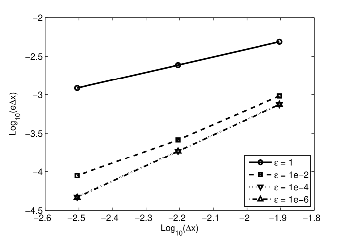
Figure 1: Convergence order of the method for $\varepsilon\in\{1,\,0.01,\,10^{-4},\,10^{-6}\}$ at time $t=0.1$.

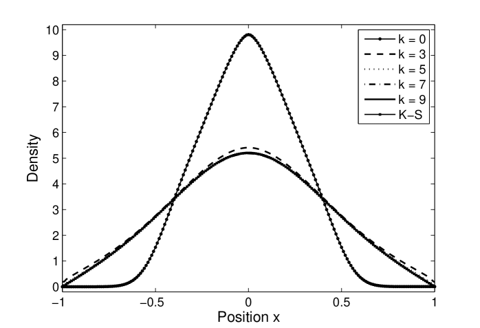
Figure 2: Density of cells at time $t=0.5$ using MM and K-S schemes for $\varepsilon=2^{-k}$ ($k\in\{0,1,2,5,9\}$).

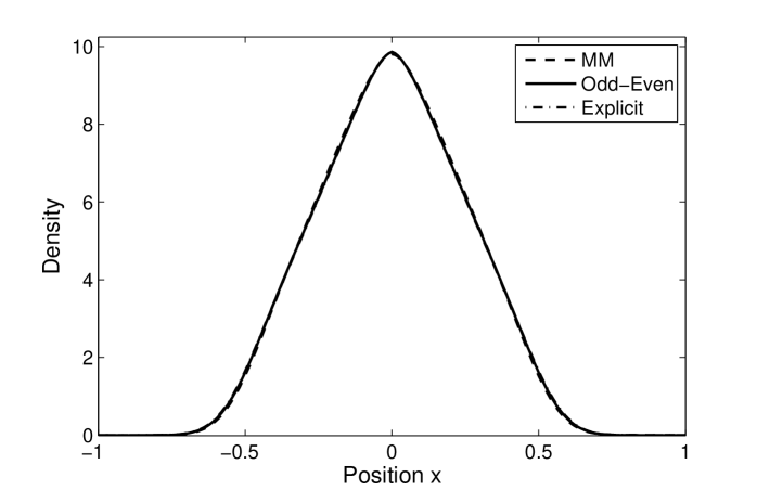
Figure 3: Density of cells at time $t=0.5$ obtained with MM, Odd-Even and Explicit schemes for $\varepsilon=1$.

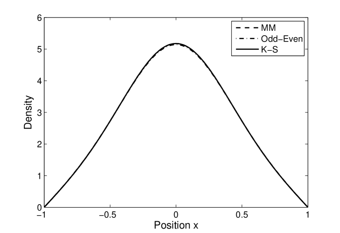
Figure 4: Density of cells at time $t=0.5$ obtained with MM, Odd-Even and Explicit schemes for $\varepsilon=10^{-6}$.

We also illustrate the behaviour of the methods in macroscopic regime. We compare in Figure 4 the density of cells obtained for $\varepsilon=10^{-6}$ with the MM, Odd-Even and K-S schemes at time $t=0.5$. As expected, for both schemes, the results are quite the same.

We investigate the time evolution of the density using the MM scheme in different regimes ($\varepsilon=1,10^{-6}$). The results are shown in Figure 5 and Figure 6. In each case, the density seems to evolve to a stationary solution.

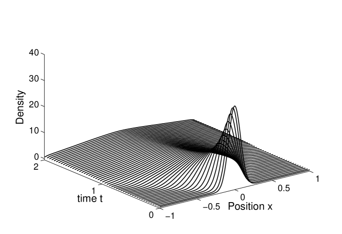
Figure 5: Evolution of the cell Density using MM scheme for $\varepsilon=1$.

Figure 6: Evolution of the cell Density using MM scheme for $\varepsilon=10^{-6}$.

6 Closure looking ahead at research perspectives

This paper has developed a computational approach to a class of pattern formation models derived from the celebrated Keller-Segel model obtained by the underlying description delivered by generalized kinetic theory methods. The derivation is based on a decomposition with two scales, namely the microscopic and the macroscopic one technically related, as we have seen, by suitable small parameters accounting for the time and space dynamics.

The novelty of our paper is that the computational scheme which follows precisely the derivation hallmarks by using the same decomposition and parameters. This idea improves the stability properties of the solutions with respect to classical approaches known in the literature. However, without repeating concepts already mentioned in the previous sections, we wish to stress that this method can contribute to future developments also related to applications. In fact, the need of new models in biology is presented in [3] and [5] to account for a broad variety of biological phenomena. Moreover, it is shown in [5] that the so-called micro-macro decomposition can lead to an interesting variety of models such as models of angiogenesis phenomena.

Therefore, modeling and computational methods can march together thus contribution to a deeper understanding of the specific features of the two different, however, related fields. Indeed, we have in mind not only applications in biology, but also to the dynamics of self-propelled particles such as those of vehicular traffic as it has been recently shown [41] how macroscopic models can be derived from the kinetic description using precisely the micro-macro decomposition treated in this present paper.

References

- [1] C.S. Patlak, Random walk with persistence and external bias, Bull. Math. Biol. Biophys., vol. 15, pp. 311-338, 1953.
- [2] E.F. Keller and L.A. Segel, Traveling band of chemotactic bacteria: A theoretical analysis, J. Theor. Biol., vol. 30, pp. 235-248, 1971.
- [3] T. Hillen and K.J. Painter, A users guide to PDE models for chemotaxis, J. Math. Biol., vol. 58 pp. 183-217, 2009.
- [4] D. Horstmann, From 1970 until present: The Keller–Segel model in chemotaxis and its consequences. I, Jahresberichte Deutsch. Math.-Verein, vol. 105, pp. 103-165, 2003.
- [5] N. Bellomo, A. Bellouquid, Y. Tao, and M. Winkler, Toward a mathematical theory of Keller-Segel models of pattern formation in biological tissues, Math. Models Methods Appl. Sci. , vol. 25, no. 09, pp. 1663-1763, 2015.
- [6] H. G. Othmer, S. R. Dunbar, and W. Alt, Models of dispersal in biological systems, J. Math. Biol., vol. 26, pp. 263-298, 1988.
- [7] H. G. Othmer and A. Stevens, Aggregation, blowup, and collapse: The ABC’s of taxis in reinforced random walks, SIAM J. Appl. Math., vol. 57, no. 4, pp. 1044-1081, 1997.
- [8] N. Bellomo, A. Bellouquid, J. Nieto, and J. Soler, Multicellular growing systems: Hyperbolic limits towards macroscopic description, Math. Models Methods Appl. Sci., vol. 17, pp. 1675-1693, 2007.
- [9] N. Bellomo, A. Bellouquid, N. Nieto, and J. Soler, Modeling chemotaxis from closure moments in kinetic theory of active particles, Discrete Contin. Dyn. Syst., Ser. B, vol. 18, pp. 847-863, 2013.
- [10] A. Bellouquid and E. De Angelis, From Kinetic Models of Multicellular Growing Systems to Macroscopic Biological Tissue Models, Nonlinear Analysis: Real World Applications, vol. 12, pp. 1111–1122, 2011.
- [11] F. Filbet, P. Laurençot and B. Perthame, Derivation of hyperbolic models for chemosensitive movement, J. Math. Biol., vol. 50, pp. 189-207, 2005.
- [12] T. Hillen, On the -moment closure of transport equation: The Cattaneo approximation, Discrete Contin. Dyn. Syst., Ser. B, vol. 4, pp. 961-982, 2004.
- [13] S. Jin, Efficient asymptotic-preserving (AP) schemes for some multiscale kinetic equations, SIAM J. Sci. Comput., vol. 21, no. 2, pp. 441-454, 1999.
- [14] N. Crouseilles, P. Degond, and M. Lemou, A hybrid kinetic/fluid model for solving the gas dynamics Boltzmann-BGK equation, J. Comput. Phys., vol. 199, pp. 776-808, 2004.
- [15] P. Degond, S. Jin, and L. Mieussens, A smooth transition model between kinetic and hydrodynamic equations, J. Comput. Phys., vol.209 pp. 665-694, 2005.
- [16] L. Pareschi and R.E. Caflisch, An implicit Monte Carlo method for rarefied gas dynamics. I. The space homogeneous case, J. Comput. Phys., vol. 154, pp. 90-116, 1999.
- [17] L. Pareschi and G. Russo, Asymptotic preserving Monte Carlo methods for the Boltzmann equation, Transp. Theory Stat. Phys., vol. 29, pp. 415-430, 2000.
- [18] L. Pareschi and G. Russo, Time relaxed Monte Carlo methods for the Boltzmann equation, SIAM J. Sci. Comput., vol. 23 pp. 1253-1273, 2001.
- [19] J. A. Carrillo and B. Yan, An Asymptotic Preserving Scheme for the Diffusive Limit of Kinetic systems for Chemotaxis, Multiscale Model. Simul., vol. 11, no. 1, pp. 336-361, 2013.
- [20] J.-M. Coron and B. Perthame, Numerical passage from kinetic to fluid equations, SIAM J. Numer. Anal., vol. 28, pp. 26-42, 1991.
- [21] S. Jin and L. Pareschi, Discretization of the multiscale semiconductor Boltzmann equation by diffusive relaxation schemes, J. Comput. Phys., vol. 161, pp. 312-330, 2000.
- [22] S. Jin, L. Pareschi, and G. Toscani, Uniformly accurate diffusive relaxation schemes for multiscale transport equations, SIAM J. Numer. Anal., vol. 38, no. 3, pp. 913-936, 2001.
- [23] A. Klar and C. Schmeiser, Numerical passage from radiative heat transfer to nonlinear diffusion models, Math. Models Methods Appl. Sci., vol. 11, pp. 749-767, 2001.
- [24] F. Filbet and S. Jin, A class of asymptotic preserving schemes for kinetic equations and related problems with stiff sources, J. Comput. Phys., vol.229, 7625-7648, 2010.
- [25] F. Filbet and S. Jin, An asymptotic preserving scheme for the ES-BGK model for the Boltzmann equation, J. Sci. Comp., vol. 46, pp. 204-224, 2011.
- [26] S. Jin and B. Yan, A class of asymptotic-preserving schemes for the Fokker-Planck-Landau equation, J. Comput. Phys., vol. 230, pp. 6420-6437, 2011.
- [27] B. Yan and J. Shi, A successive penalty-based asymptotic-preserving scheme for kinetic equations, SIAM J. Numer. Anal., vol.35, no. 1, pp. 150-172, 2013.
- [28] T.P. Liu and S.H. Yu, Boltzmann equation: micro-macro decompositions and positivity of shock profiles, Communications in Mathematical Physics, vol. 246, no. 1, pp. 133-179, 2004.
- [29] M. Bennoune, M. Lemou, and L. Mieussens, Uniformly stable numerical schemes for the Boltzmann equation preserving the compressible Navier-Stokes asymptotics, J. Comput. Phys., vol. 227, pp. 3781-3803, 2008.
- [30] M. Bennoune, M. Lemou, and L. Mieussens, An asymptotic preserving scheme for the Kac model of the Boltzmann equation in the diffusion limit, Continuum Mechanics and Thermodynamics, vol. 21, pp. 401-421, 2009.
- [31] J. A. Carrillo, T. Goudon, P. Lafitte, and F. Vecil, Numerical schemes of diffusion asymptotics and moment closure for kinetic equations, J. Sci. Comput., vol. 35, pp. 113-149, 2008.
- [32] A. Crestetto, N. Crouseilles, and M. Lemou, Kinetic/fluid micro-macro numerical schemes for Vlasov-Poisson-BGK equation using particles, Kinet. Relat. Models, vol. 5, no. 4, pp. 487-816, 2012.
- [33] N. Crouseilles and M. Lemou, An asymptotic preserving scheme based on a micro-macro decomposition for collisional Vlasov equations: diffusion and high-field scaling limits, Kinet. Relat. Models, vol. 4, pp. 441–477, 2011.
- [34] S. Jin and Y. Shi, A micro-macro decomposition based asymptotic-preserving scheme for the multispecies Boltzmann equation, SIAM J. Sci. Comput., vol.31, pp. 4580-4606, 2010.
- [35] M. Lemou and L. Mieussens, A new asymptotic preserving scheme based on micro-macro formulation for linear kinetic equations in the diffusion limit, SIAM J. Sci. Comput., vol. 31, pp. 334-368, 2008.
- [36] M. Lemou and F. Méhats, Micro-macro schemes for kinetic equations including boundary layers, SIAM J. Sci. Comput., vol. 34, pp. 734-760, 2012.
- [37] T. Hillen and H.G. Othmer, The diffusion limit of transport equations derived from velocity jump processes, SIAM J. Appl. Math., vol. 61, pp. 751-775, 2000.
- [38] H.G. Othmer and T. Hillen, The diffusion limit of transport equations II: chemotaxis equations, SIAM J. Appl. Math., vol.62, pp. 1222-1250, 2002.
- [39] F. A. Chalub, P. Markowich, B. Perthame, and C. Schmeiser, Kinetic Models for Chemotaxis and their Drift-Diffusion Limits, Monatsh. Math., vol. 142, pp. 123-141, 2004.
- [40] N. Saito, Conservative numerical schemes for the Keller-Segel system and numerical results, RIMS Kôkyûroku Bessatsu, vol. 15, pp. 125-146, 2005.
- [41] N. Bellomo, A. Bellouquid, J. Nieto, and J. Soler, On the multi scale modeling of vehicular traffic: from kinetic to hydrodynamics, Discrete Contin. Dyn. Syst., Ser. B, vol.19, pp. 1869-1888, 2014.