Tensor anisotropy as a tracer of cosmic voids

Abstract

We present a new method to find voids in cosmological simulations based on the tidal and the velocity shear tensors definitions of the cosmic web. We use the fractional anisotropy (FA) computed from the eigenvalues of each web scheme as a void tracer. We identify voids using a watershed transform based on the local minima of the FA field without making any assumption on the shape or structure of the voids. We test the method on the Bolshoi simulation and report on the abundance and radial averaged profiles for the density, velocity and fractional anisotropy. We find that voids in the velocity shear web are smaller than voids in the tidal web, with a particular overabundance of very small voids in the inner region of filaments/sheets. We classify voids as subcompensated/overcompansated depending on the absence/presence of an overdense matter ridge in their density profile, finding that close to $65\%$ and $35\%$ of the total population are classified into each category, respectively. Finally, we find evidence for the existence of universal profiles from the radially averaged profiles for density, velocity and fractional anisotropy. This requires that the radial coordinate is normalized to the effective radius of each void. Put together, all these results show that the FA is a reliable tracer for voids, which can be used in complementarity to other existing methods and tracers.

1 Introduction

Cosmic voids are regarded as one of the most striking features of the Universe on its larger scales ever since they were found in the first galaxy surveys (Chincarini & Rood, 1975; Gregory & Thompson, 1978; Einasto et al., 1980a, b; Kirshner et al., 1981; Zeldovich et al., 1982; Kirshner et al., 1987). However, due to the large volume extension of void regions ($\sim 5-10\ \mbox{Mpc}h^{-1}$), statistically meaningful catalogues of voids (Pan et al., 2012; Sutter et al., 2012; Nadathur & Hotchkiss, 2014) have only become available through modern galaxy surveys such as the two-degree field Galaxy Redshift Survey (2dF) (Colless et al., 2001, 2003) and the Sloan Digital Sky Survey (SDSS)(York et al., 2000; Abazajian et al., 2003). These observational breakthroughs generated a great interest in the last decade to study voids (Hoyle & Vogeley, 2004; Croton & et al., 2004; Padilla et al., 2005; Rojas et al., 2005; Ceccarelli et al., 2006; Patiri et al., 2006; Tikhonov, 2006; Patiri et al., 2006; Tikhonov, 2007; von Benda-Beckmann & Müller, 2008; Foster & Nelson, 2009; Ceccarelli et al., 2013; Paz et al., 2013; Sutter et al., 2014).

On the theoretical side, the basic framework that explains the origin of voids was established in the seminal work of Zel’dovich (1970) and refined in the following decades. The first detailed theoretical models describing formation, dynamics and properties of voids (Hoffman & Shaham, 1982; Icke, 1984; Bertschinger, 1985; Blumenthal et al., 1992) were complemented and extended by numerical studies (Martel & Wasserman, 1990; Regos & Geller, 1991; van de Weygaert & van Kampen, 1993; Dubinski et al., 1993; Bond et al., 1996). Currently, the most popular approach to study voids relies on N-body simulations. For an extensive compilation of previous numerical works we refer the reader to Colberg et al. (2008).

The relevance of voids to cosmological studies can be summarized in three aspects (Platen et al., 2007). Firstly, voids are a key ingredient of the Cosmic Web. They dominate the volume distribution at large scales and compensate overdense structures in the total matter budget. Secondly, voids provide a valuable resource to estimate cosmological parameters as their structure and dynamics are sensitive to them. Finally, they are a largely pristine environment to test galaxy evolution.

Although visual recognition of voids in galaxy surveys and simulations is possible in most cases, we need a clear algorithmic identification procedure to make statistical studies. Nevertheless, the community has not reached yet an unambiguous definition of cosmic voids. There are many different void finding techniques in the literature (for a detailed comparison of different schemes, see the publication on the results of the Void Finder Comparison Project Colberg et al. (2008)). In spite of the diversity of existing schemes, they can be roughly classified into two types: point-based and field-based. There are geometric schemes based on point distributions (either real or redshift space) f galaxies in surveys or dark matter halos in simulations (Kauffmann & Fairall, 1991; Müller et al., 2000; Gottlöber et al., 2003; Hoyle & Vogeley, 2004; Brunino et al., 2007; Foster & Nelson, 2009; Micheletti et al., 2014; Sutter et al., 2015). While other schemes are based on the smooth and continuous matter density field either from simulations or from reconstruction procedures on surveys (Plionis & Basilakos, 2002; Colberg et al., 2005; Shandarin et al., 2006; Platen et al., 2007; Neyrinck, 2008; Muñoz-Cuartas et al., 2011; Neyrinck et al., 2013; Ricciardelli et al., 2013). Our work follows the tradition of the second kind of schemes.

Here we introduce a new algorithm to define voids over the continuous matter density or velocity distribution defined on a fixed and homogeneous spatial grid. The algorithm uses the results from two tensorial schemes used to classify the cosmic web. The first (the T-Web) is based on the Hessian of the gravitational potential or tidal tensor (Hahn et al., 2007; Forero-Romero et al., 2009). The second (the V-web) is based on the velocity shear tensor (Hoffman et al., 2012). Our procedure allows for a description of a void internal structure beyond a simple definition of a void as an underdense region in the large-scale matter distribution. The tidal and the shear tensors encode more information than the density/velocity fields as they trace the collapsing or expanding nature of the matter field, which defines the dynamics of the Cosmic Web.

The tracer that we use to define the voids is the fractional anisotropy (FA) computed from the set of eigenvalues of the tensor under consideration. The FA was initially introduced by Basser (1995) to quantify the anisotropy degree of the diffusivity of water molecules through cerebral tissue in nuclear magnetic resonance imaging, thereby allowing to detect structures that restrict the otherwise isotropic Brownian movement of water molecules. Taking into account that this process is identical to the velocity shear in the large-scale matter distribution, Libeskind et al. (2013) introduced the concept of the FA in the context of Cosmic Web classification schemes.

In the next sections (§2 and §3) we establish the FA as a void tracer and then proceed to identify individual voids as basins of FA local minima. At this point we implement a watershed transform algorithm (Beucher & Lantuejoul, 1979; Beucher & Meyer, 1993) which has been used to define voids as catching basins of local minima of the density field (Platen et al., 2007; Neyrinck, 2008). Finally we find and charachterize voids in a N-body (§4 and §5) using density, velocity and fractional anisotropy profiles. We use these results to comment on the qualities of our algorithm (§6).

2 Algorithms to find the Cosmic Web

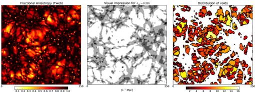
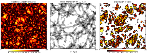
Figure 1: Different fields in a slice of $1{{h^{-1}{\rm Mpc}}}$ width in the Bolshoi simulation. Top/bottom panels correspond to the T-Web/V-Web. Fractional Anisotropy field (left); cosmic web classification (middle) for a given value of the threshold eigenvalue $\lambda_{\rm th}$ where voids are white, sheets are light gray, filaments are dark gray and knots are black; individual voids (right) found by the a watershed algorithm on the Fractional Anisotropy field. Colours in the right panel correspond with the effective radius of each void.

Our new void finding method is based on two existing cosmic web classification schemes that work on cosmological N-body simulations. Both schemes depend on the construction of tensors based on the Hessian of the potential (T-Web scheme) and the shear of the velocity (V-Web scheme). These algorithms have been used to develop other kind of studies such as the alignment of the shape, spin and peculiar velocity of dark matter halos with the cosmic web (Libeskind et al., 2013; Forero-Romero et al., 2014). Here we summarize the most relevant aspects of each scheme. We refer the reader to the papers of Forero-Romero et al. (2009) (T-Web) and Hoffman et al. (2012) (V-Web) for detailed descriptions.

2.1 The tidal web (T-Web)

This scheme was initially proposed by Hahn et al. (2007) to find the Cosmic Web based on the tidal tensor. The tidal tensor allows a classification in terms of the orbital dynamics of the matter field. This approach extends to second-order the equations of motion around local minima of the gravitational potential. The second-order term corresponds to the tidal tensor, which is defined as the Hessian matrix of the normalized gravitational potential

$$T_{\alpha\beta}=\frac{\partial^{2}\phi}{\partial x_{\alpha}\partial x_{\beta}},$$ (1)

where the physical gravitational potential has been rescaled by a factor of $4\pi G\bar{\rho}$ in such a way that $\phi$ satisfies the following Poisson equation

$$\nabla^{2}\phi=\delta,$$ (2)

with $\bar{\rho}$ the average density in the Universe, $G$ the gravitational constant and $\delta$ the dimensionless matter overdensity.

Since the tidal tensor can be represented by a real and symmetric $3\times 3$ matrix, it is always possible to diagonalize it and obtain three real eigenvalues $\lambda_{1}\geq\lambda_{2}\geq\lambda_{3}$ with its corresponding eigenvectors ${\bf u}_{1}$, ${\bf u}_{2}$, ${\bf u}_{3}$. The eigenvalues are indicators of the local orbital stability in each direction ${\bf u}_{i}$. The sign of the eigenvalues can be used to classify the Cosmic Web. The number of positive (stable) or negative (unstable) eigenvalues allows to label a location into one of the next four types of environment: voids (3 negative eigenvalues), sheets (2), filaments (1) and knots (0).

A modification to this scheme was introduced by Forero-Romero et al. (2009) by means of a relaxation of the stability criterion. The relative strength of each eigenvalue is no longer defined by the sign, but instead by a threshold value $\lambda_{\rm th}$ that can be tuned in such a way that the visual impression of the web-like matter distribution is reproduced.

2.2 The velocity web (V-Web)

The V-web scheme for environment finding introduced by Hoffman et al. (2012) is based on the local velocity shear tensor calculated from the smoothed dark matter velocity field in the simulation. This tensor is given by the following expression

$$\Sigma_{\alpha\beta}=-\frac{1}{2H_{0}}\left(\frac{\partial v_{\alpha}}{\partial x_{\beta}}+\frac{\partial v_{\beta}}{\partial x_{\alpha}}\right),$$ (3)

where $v_{\alpha}$ and $x_{\alpha}$ represent the $\alpha$ component of the comoving velocity and position, respectively. Like the tidal tensor, $\Sigma_{\alpha\beta}$ can be represented by a $3\times 3$ symmetric matrix with real values, making it possible to find three real eigenvalues and its corresponding eigenvectors.

In this case we also use the relative strength of the three eigenvalues with respect to a threshold value $\lambda_{th}$ to classify the cosmic web in the four web types already mentioned.

Usually, the threshold $\lambda_{th}$ is a free parameter that is tuned to reproduce the visual appearance of the comic web. However, in this paper this threshold does not play any role in our computations. In Figure 2 we offer a threshold estimate (from the FA=$0.95$ as a function of $\lambda_{1}$, this choice is explained in the next section) only as a guide to readers familiar with its meaning.

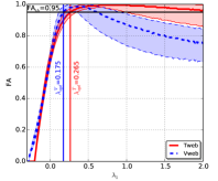
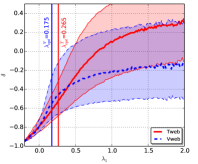
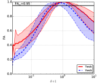
Figure 2: Fractional Anisotropy as a function of the overdensity (left) and the eigenvalue $\lambda_{1}$ (middle), and density contrast (right) as a function of the eigenvalue $\lambda_{1}$ for each web scheme (T-Web, continuous lines. V-Web, dashed lines). Fractional Anisotropy as a function of $\lambda_{1}$ (left), overdensity as a function of $\lambda_{1}$ (middle) and Fractional Anisotropy as a function of the overdensity (right). Thick central lines are the median and filled regions include $50\%$ of the cells in each bin. The left panel shows the tight correlation between FA and $\lambda_{1}$ in voids. In the middle and right panel we show the equivalent eigenvalue threshold for the T-Web and V-web corresponding to FA=$0.95$. The right panel confirms that underdense regions can be identified with Fractional Anisotropy values less than $0.95$. For this reason we define voids to be composed by cells with Fractional Anisotropy equal or less than this value. The threshold $\lambda_{\rm th}$ on the eigenvalues does not influence our results. We show it as a guide to readers familiar with the order of magnitude expectation for this quantity.

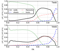
Figure 3: Volume of each environment per FA ($dV_{i}/dFA,\ \ i=v,s,f,k$) normalized by the total volume per FA ($dV/dFA$). Top/bottom corresponds to the T-Web/V-Web. For a given value of the FA, each line represents the volume contribution of the respective environment to the total volume with the same FA value. Above FA=0.95, only sheets and filaments contribute to all the volume of the simulation within that range of FA.

3 A new void finding technique

3.1 The fractional anisotropy

The fractional anisotropy (FA), as developed by Basser (1995), was conceived to quantify the anisotropy of the diffusivity of water molecules through cerebral tissue in nuclear magnetic resonance imaging. In this manner, barriers such as microtubules and cell membranes, that restrict the otherwise isotropic Brownian motion of water molecules, can be detected. In a cosmological context, the problem of finding structures is very similar, where filaments and sheets restrict the otherwise isotropic collapsing/expanding dynamics of the matter. Taking this into account, we present here the FA, much in the same way as Libeskind et al. (2013), to use it as a tracer of cosmic voids.

The FA is defined as follows

$${\mathrm{FA}}=\frac{1}{\sqrt{3}}\sqrt{\frac{(\lambda_{1}-\lambda_{3})^{2}+(\lambda_{2}-\lambda_{3})^{2}+(\lambda_{1}-\lambda_{2})^{2}}{\lambda_{1}^{2}+\lambda_{2}^{2}+\lambda_{3}^{2}}},$$ (4)

where the eigenvalues can be taken from either the T-Web or the V-Web (FA-T-Web and FA-V-Web respectively). Such as it is defined, FA$=0$ corresponds to an isotropic distribution ($\lambda_{1}=\lambda_{2}=\lambda_{3}$) and FA$=1$ to a highly anisotropic distribution.

In the left and middle panels of Fig. 1 we show the FA field and web classification for both web schemes over a slice of an N-body simulation (described in Section 4). Comparing these two panels we see that voids and knots (white and black in the middle panel of Fig. 1) display low FA values at their centres, becoming gradually more anisotropic at outer regions. On the other hand the filamentary structure (grey in the middle panel of Fig. 1) is traced by middle to high FA values. This characteristic is the key to use the FA as a tracer of cosmic voids.

3.2 Fractional anisotropy as a void tracer

Voids are regions where $\lambda_{3}\leq\lambda_{2}\leq\lambda_{1}\leq\lambda_{\rm th}$. This implies that a void is completely fixed by the relative strength of the $\lambda_{1}$ eigenvalue with respect to the threshold. As we increase/decrease the threshold value $\lambda_{\rm th}$, voids increase/decrease progressively through contours of increasing/decreasing $\lambda_{1}$. Voids are thus characterized by low values of both FA and $\lambda_{1}$.

In Fig. 2 we show that the these two values are correlated. The left panel shows the correlation between the FA and $\lambda_{1}$ and the middle panel between the overdensity $\delta$ and $\lambda_{1}$. The right panel shows the correlation between $\delta$ and the FA. This shows that the density has a larger scatter at fixed $\lambda_{1}$ than the FA, yet large and small values of the density remain still associated to low values of the FA.

At this point, the eigenvalue $\lambda_{1}$ and the FA appear to be equally potential candidates for tracing cosmic voids, however, the eigenvalue $\lambda_{1}$ presents, along with the overdensity, an undesirable feature for a void tracer. As we move out from inner parts of voids to outer parts, $\lambda_{1}$ and $\delta$ increase monotonically making unclear where to set the void boundary, while for low density regions ($\delta<1$) the FA traces the boundary where anisotropic collapsing regions begin to dominate, i.e. at the ridge reached around $\delta=0$ as shown in the right panel of Fig. 2. According to Fig. 3 these anisotropic areas are mainly associated to sheets and, to a lesser extent, filaments.

From Figs. 1 and 2 we conclude that the FA is a good tracer of voids as it is almost perfectly correlated with low values of $\lambda_{1}$. We propose that voids should be composed completely by regions of FA$<0.95$. If we increase the values of $\lambda_{1}$ from its minimum until it we reach FA$=0.95$ in 2 we find that this correspond to critical values of $\lambda_{1}^{T}=0.265$ and $\lambda_{1}^{V}=0.175$ for the T-Web and V-Web, respectively. This means that setting $\lambda_{th}$ to either $\lambda_{1}^{T}$/$\lambda_{1}^{V}$ automatically produces voids with all the cells FA$<0.95$. The middle panels in Fig. 1 show the web classification for this choice of $\lambda_{th}$, demonstrating that this FA level is a reasonable choice to define voids.

3.3 Defining voids with a watershed algorithm

The previous Section shows that FA is a good void tracer, but how should we actually define the boundary of individual voids? For this purpose, we use the watershed transform algorithm (Beucher & Lantuejoul, 1979; Beucher & Meyer, 1993) to identify a void as the basin of FA local minima with boundaries of FA$=0.95$. The advantage of this definition is that it does not require any assumption on the shape and/or morphology of the tentative voids.

However, there are two main differences in our approach with respect to other watershed implementations. First, the watershed technique commonly uses the density field instead of the FA field as we do here (Platen et al., 2007; Neyrinck, 2008). Second, we estimate all relevant quantities on a Cartesian mesh of fixed cell size, while other works use an adaptive Delaunay tessellation (Schaap & van de Weygaert, 2000). Nevertheless, in our case the average number of particles per cell is large enough ($512$ particles/cell) ensuring that the lowest density regions are sampled with at least $\sim 10$ particles ($\delta\sim-0.98$), which seems to avoid spurious results from a noisy density field sampling.

The watershed algorithm also needs a threshold value to reduce spurious features and prevent void hierarchization. If the density field is used, a typical threshold is $\delta=-0.8$ (Platen et al., 2007), which means that, given two neighbouring voids, if the mean value of the density across their common boundary is below that threshold, the two voids are merged. In our case we have to find a corresponding FA value to define this threshold.

In the right panel of Fig. 2 we see how the FA correlates with the matter overdensity. A value of $\delta=-0.8$ corresponds to a value of FA$\sim 0.65$ regardless of the web-finding scheme. This is the value we choose to remove ridges between two watershed voids. The right column in Fig. 1 shows all the individual voids that have been identified using the watershed algorithm on the FA field.

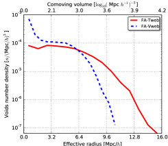
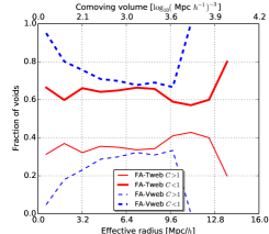
Figure 4: Left panel, void size distribution. Right panel, fraction of overcompensated/subcompensated ($C>1/C<1$)voids as a function of the effective radius. The continuous (dashed) curves correspond to the T-Web (V-Web). The abundance for small (${{r_{\mbox{\tiny eff}}}}<2.0{{h^{-1}{\rm Mpc}}}$) overcompensated voids shoots up in the V-Web scheme. We provide in the body of the paper two reasons for this behaviour.

4 Numerical Simulation

We use the Bolshoi simulation to test our void finding method. This simulation follows the non-linear evolution of a dark matter density field on a cubic volume of size $250$$h^{-1}$Mpc sampled with $2048^{3}$ particles. The cosmological parameters in the simulation are $\Omega_{\rm m}=0.27$, $\Omega_{\Lambda}=0.73$, $h=0.70$, $n=0.95$ and $\sigma_{8}=0.82$ for the matter density, cosmological constant, dimensionless Hubble parameter, spectral index of primordial density perturbations and normalization for the power spectrum, respectively. These values are consistent with the ninth year of data of the Wilkinson Microwave Anisotropy Probe (WMAP) (Hinshaw et al., 2013). For more detailed technical information about the simulation, see Klypin et al. (2011).

We use data for the cosmic web identification that is publicly available through the MultiDark database http://www.multidark.org/MultiDark/ which is described in Riebe et al. (2013). Here we briefly describe the process to obtain the data. For details see Forero-Romero et al. (2009) (T-Web); Hoffman et al. (2012); Forero-Romero et al. (2014) (V-Web). This data is based on a cloud-in-cell (CIC) interpolation of the density and velocity fields of the simulation onto a grid of $256^{3}$ cells, corresponding to a spatial resolution of $0.98$$h^{-1}$Mpc per cell side. These fields are smoothed with a gaussian filter with a width of $\sigma=0.98$$h^{-1}$Mpc. The tidal and shear tensors and corresponding eigenvalues are computed through finite-differences over the potential and velocity fields.

5 Results

We limit our results to voids with effective radius larger than the smoothing length of the density field, i.e. $\sim 1$$h^{-1}$Mpc. For smaller interpolation/smoothing scales the shot noise in the low density regions starts to be noticeable. With that choice we find a void volume filling fraction $54.88\%$ and $47.06\%$ for the FA-Vweb and the FA-Tweb, respectively. For larger smoothing scales ($>5{{h^{-1}{\rm Mpc}}}$) the density and shear fields tend to be Gaussian and therefore follow closely the analytical environment abundance predictions for Gaussian random fields (Forero-Romero et al., 2009; Alonso et al., 2015). In this paper we limit ourselves to a smoothing scale $\sim 1$ $h^{-1}$Mpc.

In the following subsections we describe the results for the size distribution and different radial profiles for all our samples.

5.1 The void size distribution

Void shapes exhibit a wide range of geometries. To define their size we use its equivalent spherical radius or effective radius, defined as ${{r_{\mbox{\tiny eff}}}}=[3/(4\pi)V]^{1/3}$, with $V$ the total volume of the void computed from the individual grid cells assigned to the void. In Fig. 4 we show the void size distributions for the T-Web and the V-Web.

We see that the void distribution for the T-Web is broadly consistent with the expectations from a two-barrier problem (Sheth & van de Weygaert, 2004). The formation of large voids is limited by the void-in-void mechanism (first barrier) where large voids are constituted hierarchically of smaller ones. In turn, the formation of small voids is damped by the void-in-cloud mechanism (second barrier), where nearby collapsing structures limit the abundance of small embedded voids.

We also find that the V-Web scheme produces an over-abundance of small voids compared to T-Web. A large number of these small voids are embedded in overdense regions. They are already visible in the middle panel of Fig. 1 as tiny white bubbles located inside sheets. The existence of these small voids can be explained by dynamics of shell crossing in collapsing sheets as discussed in Hoffman et al. (2012). The main argument is that as matter collides into a pancake-like fashion crossing sheets encounter each other at the symmetry plane. This effectively gives a positive divergence in the velocity field, resulting in a void identification by the V-Web algorithm.

Comparing the abundance of large voids in the two web schemes, we find that the largest voids in the V-Web have ${{r_{\mbox{\tiny eff}}}}\sim 10$$h^{-1}$Mpc, while the T-Web scheme includes voids as large as ${{r_{\mbox{\tiny eff}}}}\sim 15$$h^{-1}$Mpc. This suggests that large voids in the T-Web scheme have a velocity structure that splits them in the V-Web. This increased granularity in the velocity structure of voids is evident in the left and right panels of Fig. 1.

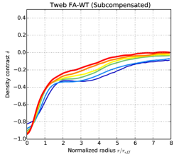
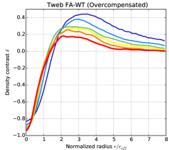
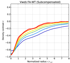
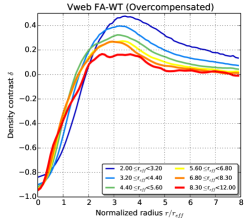
Figure 5: Spherically averaged radial density profiles for stacked voids with different effective radii. The sample is split into subcompensated and overcompensated voids (right and left) for the web schemes T-Web and V-Web (top and bottom).

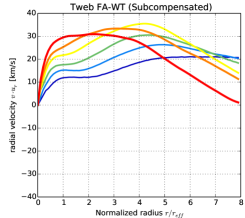
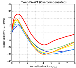
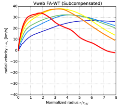
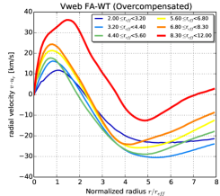
Figure 6: Spherically averaged radial velocity profiles for stacked voids with different effective radii. The sample is split into subcompensated and overcompensated voids (right and left) for the web schemes T-Web and V-Web (top and bottom).

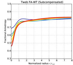
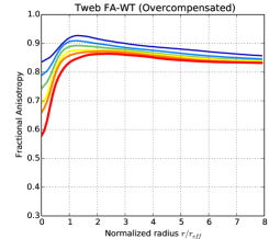
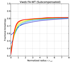
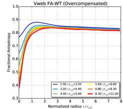
Figure 7: Spherically averaged Fractional Anisotropy profiles for stacked voids with different effective radii. The sample is split into subcompensated and overcompensated voids (right and left) for the web schemes T-Web and V-Web (top and bottom).

5.2 Subcompensated and overcompensated voids

We find that voids are distributed in two different families differentiated by the presence/absence of an overdense matter ridge in their density profiles. To discriminate each void in one of the families we use the compensation index $C$ It is defined as the mass of a void enclosed in a spherical volume of radius $R$ and normalized by the mass of the same volume assuming it is filled by matter with the mean background density.

$$C=\frac{M_{v}}{\overline{M}}=\frac{3}{2R^{3}}\int_{0}^{R}[\delta(r)+1]r^{2}dr$$ (5)

We choose an integration radius of $R=4{{r_{\mbox{\tiny eff}}}}$, that is large enough to enclose the compensation ridge for a typical void in case there is one. This leads us to voids with $C>1$ having more mass than expected, constituting the family of overcompensated voids. These voids generally exhibit a compensation ridge associated to dense nearby structures. In the same fashion, voids with $C<1$ constitute the family of subcompensated voids.

In Fig. 5 we show the density and velocity profiles of voids split in these two families. In the left column it becomes clear the difference between sub- and overcompensated voids. Table 1 lists the number of voids in each effective radius bin for the two web finding methods.

	Tweb		Vweb
${\bf{{r_{\mbox{\tiny eff}}}}}$[$h^{-1}$Mpc]	$\bf{C<1}$	$\bf{C>1}$	$\bf{C<1}$	$\bf{C>1}$
$<2.0$	997	495	13480	711
$2.0-3.2$	791	471	2581	583
$3.2-4.4$	941	469	2168	656
$4.4-5.6$	869	467	1934	724
$5.6-6.8$	769	395	1287	584
$6.8-8.3$	665	362	700	315
$8.3-12.0$	587	333	123	61
$>12.0$	29	23	0	0
total	5648	3015	22273	3634

Table 1: Number of voids for each bin of effective radius and for subcompensanted and overcompansated samples.

5.3 Density profiles

We calculate the contrast density, radial-projected velocity and FA profiles. For this purpose we stack voids with similar effective radius. We also compute the profiles separately for subcompensated and overcompensated voids. For each void, we take the distance of each member cell to the void centre along with the properties of interest. We normalize the radial distance with the effective radius and add the result to the stack.

Fig. 5 shows the results of stacked density profiles for different void sizes. We calculate the profile out to a radius $8\ {{r_{\mbox{\tiny eff}}}}$ to capture the point where the overdensity reaches the mean value.

The first interesting result is the overdensity value at the void’s centre. We find that larger voids have a lower overdensity value. The largest voids ($8.3-12\ {{h^{-1}{\rm Mpc}}}$) have an underdensity $\delta\sim-0.95$ while smaller voids ($2-3.2\ {{h^{-1}{\rm Mpc}}}$) fall around $\delta\sim-0.8$ at their centres. This holds for both web schemes. These values are consistent with most of the void finding schemes based on smooth and continuous fields from simulation or reconstruction procedures on surveys (Plionis & Basilakos, 2002; Colberg et al., 2005; Shandarin et al., 2006; Platen et al., 2007; Neyrinck, 2008; Muñoz-Cuartas et al., 2011; Ceccarelli et al., 2013; Paz et al., 2013; Neyrinck et al., 2013; Ricciardelli et al., 2013), unlike geometrical approaches based on point distributions, where central density values are generally higher (Colberg et al., 2008).

A second feature about these profiles is their steepness at inner regions. In subcompensated voids, larger voids are steeper. Smaller voids exhibit moderate slopes, reaching the mean density at larger radii than larger voids. This suggests that small subcompensated voids are embedded into low density structures, while large subcompensated voids are surrounded by dense structures, reaching the mean density at lower effective radii than smaller voids. In the overcompensated case larger voids reach first both the compensation ridge and then the mean density value.

Regarding overcompensated voids, a final result is related to the height of the compensation ridge: the larger the void size, the lower the ridge height. This implies that overcompensated smaller voids are embedded in very high density regions, unlike their subcompensated counterpart, thus indicating two possibly different processes for small voids formation. Larger voids exhibit lower ridges as outer radial layers also includes all sort of structures, thus being the difference between large overcompensated and subcompensated voids less conclusive.

All the previous results hold for both finding schemes. This suggests an universal behaviour for the radial density profile in two families of subcompensated and overcompensanted voids. This goes in the same direction of recent results about the internal (Colberg et al., 2005; Ricciardelli et al., 2013) and external structure of voids (Lavaux & Wandelt, 2012; Ceccarelli et al., 2013; Paz et al., 2013; Hamaus et al., 2014). Indeed, our results extend the findings of Hamaus et al. (2014) into the range of voids with size ${{r_{\mbox{\tiny eff}}}}<10$$h^{-1}$Mpc.

5.4 Velocity profiles

In Fig. 6 we present the radial velocity profiles. Positive values correspond to outflows with respect to the centre.

We find that subcompensated voids have outflowing velocity profiles all the way up to the radius where the average radial density reaches zero. In voids with sizes ${{r_{\mbox{\tiny eff}}}}<8{{h^{-1}{\rm Mpc}}}$ the outflow is always positive, consistent with the fact that their density profiles do not reach the level $\delta=0$ in the range of explored radii. This behaviour indicates that matter is being pulled out of the void into external higher density features.

On the other hand, overcompensated voids initially exhibit outward profiles, (as expected from a low density region) and approximately at the radius of the compensation ridge, the velocity reaches a peak, decreases and becomes negative, showing the infalling flow of matter further than the compensation ridge. This shows that the high density structures associated to the compensation ridge dominate the matter flow both from inside and outside the void.

As in the density, these results are also consistent with a Universal velocity profile for voids (Paz et al., 2013; Hamaus et al., 2014).

5.5 Fractional Anisotropy profiles

Fig. 7 shows the results for the FA profiles. We find that the FA clearly magnifies the difference between the internal profile $r/{{r_{\mbox{\tiny eff}}}}<1$ and the external profile $r/{{r_{\mbox{\tiny eff}}}}>1$. Subcompensanted voids in the T-Web reach an asymptotic background value of F=$0.8$ almost right at $r/{{r_{\mbox{\tiny eff}}}}=2$. For the V-Web the results are similar, albeit with a slower trend with the effective radius. Overcompensated voids reach a maximum FA at the same effective radius $r/{{r_{\mbox{\tiny eff}}}}=1$ and decline to reach an asymptotic value of FA=$0.85$ at larger radii.

The central FA values also show a magnified trend with the void size. Large voids have lower FA values, amplifying the same trend observed with the central density value. Finally, we observe that voids in the V-Web scheme span a larger range of central FA values than in the T-Web scheme.

The difference between the radius where the density ridge is reached ($r/{{r_{\mbox{\tiny eff}}}}=3$) and the radius of the FA maxima ($r/{{r_{\mbox{\tiny eff}}}}=1$, most manifest in the T-Web voids) justifies in a more quantitative way the qualitative argument we present in sub-section 3.3 to define void boundaries in our method. Namely that as we increase the void boundary moving away from the centre, we reach first middle density walls, before reaching high density structures associated with high anisotropy. This implies that voids defined with the FA never present positive overdensities, making the FA maximum a reasonable boundary for voids compared to the traditional definition that puts the boundary at the density ridge.

We recognize that our choice produces smaller voids as compared with other voids finding methods. We consider that this has the advantage of avoiding the contamination from external structures.

6 Conclusions

In this paper we propose that the anisotropy of the eigenvalues from tidal and velocity shear tensors is a good tracer of cosmic voids. Based on this idea we go on to implement a watershed algorithm on the fractional anisotropy to find voids in a N-body cosmological simulation. We perform different test on the voids found on the anisotropy of two tensorial schemes, the T-Web and the V-web.

The first quantity we examine is the void size distribution characterized by an effective radius. We find that for the T-Web scheme the void size distribution has a shape consistent with standard expectations from a two-barrier setup. However, for the V-Web we find an overabundance of the smallest voids. This is due to two reasons. First, there are artefacts in the web finding scheme inside sheets. Second, there V-web produces smaller fragmented voids inside the largest voids found in the T-Web classification. This void fragmentation hints at a complex velocity structure in large voids compared to its simpler density/gravitational potential anatomy.

A second step in the void characterization is the separation into subcompensated and overcompensated samples. In the T-Web $35\%$ of the voids are overcompensated and $65\%$ subcompensated, meaning that they are located in denser regions with a clear delimiting ridge. For the V-web the subcompensated fraction rises to $85\%$ as the void size decreases, supporting the picture of smaller spurious voids located in medium density matter sheets.

Finally we proceed with a more detailed void characterization through the radially averaged profiles of density, radial velocity and fractional anisotropy. In this case we study separately the subcompensated and overcompensated voids, split this time in samples with different effective radii.

For the density the most interesting feature is that the profile has a similar shape for all the different void sizes once the radial coordinate is expressed in units of the effective radius. In these profiles it is evident the presence of an overdense ridge around $2<r/{{r_{\mbox{\tiny eff}}}}<3$ for the overcompensated voids. Subcompensated voids do not show such a ridge keeping its density lower than the average value up to $r/{{r_{\mbox{\tiny eff}}}}\sim 8$.

In other studies where voids are found using considerations on the density fields the ridge is, almost by definition, located around $r/{{r_{\mbox{\tiny eff}}}}\sim 1$ and the subcompensated voids reach average density around $r/{{r_{\mbox{\tiny eff}}}}\sim 3$. This indicates that voids defined by FA boundaries are smaller than voids found by density only considerations close by a radial factor of $2$.

The velocity profiles show the expected correlation with the features already observed in the density. Most notably the radial velocity goes to zero close to flat regions in the density profile and is positive around regions of increasing density with radius.

The FA profiles also show remarkable similarities inside each class of subcompensated and overcompensated voids and a close correlation with the behaviour in the density and velocity profiles. From these profiles it becomes clear that the limit of overcompensated void coincides with a ridge in of FA values close to $0.9$. This value is close to the limit FA=$0.95$ we impose in the watershed algorithm, indicating that these voids are very close to spherical. For the subcompensated voids the FA quickly increases to FA values of $\sim 0.7-0.8$ at $r/{{r_{\mbox{\tiny eff}}}}\sim 1$ to find a plateau, which is quite far from the limiting FA$=0.95$ suggesting that these voids are ellipsoidal.

Put together, the results for the radially averaged profiles support the evidence for a universal density profile. Our results extend to smaller void sizes the work done by Hamaus et al. (2014) on simulations and by Ceccarelli et al. (2013) on SDSS data.

The method we present here finds voids with reasonable properties compared to different results published in the literature. This gives support to a new tracer, the Fractional Anisotropy, to be used in the study of cosmic voids. Furthermore, the complementary physical picture in the two different web finding algorithms opens the possibilities to make a joint analysis of the tidal and dynamical structure of voids.

References

- Abazajian et al. (2003) Abazajian K., et al. (the SDSS Collaboration) 2003, AJ, 126, 2081
- Alonso et al. (2015) Alonso D., Eardley E., Peacock J. A., 2015, MNRAS, 447, 2683
- Basser (1995) Basser P., 1995, NMR in Biomedical Imaging, 8, 333
- Bertschinger (1985) Bertschinger E., 1985, ApJS, 58, 1
- Beucher & Lantuejoul (1979) Beucher S., Lantuejoul C., 1979, in Proceedings Interna- tional Workshop on Image Processing, CCETT/IRISA, Rennes, France
- Beucher & Meyer (1993) Beucher S., Meyer F., 1993, Mathematical Morphology in Image Processing. Marcel Deker, New York
- Blumenthal et al. (1992) Blumenthal G. R., da Costa L. N., Goldwirth D. S., Lecar M., Piran T., 1992, ApJ, 388, 234
- Bond et al. (1996) Bond J. R., Kofman L., Pogosyan D., 1996, Nature, 380, 603
- Brunino et al. (2007) Brunino R., Trujillo I., Pearce F. R., Thomas P. A., 2007, MNRAS, 375, 184
- Ceccarelli et al. (2006) Ceccarelli L., Padilla N. D., Valotto C., Lambas D. G., 2006, MNRAS, 373, 1440
- Ceccarelli et al. (2013) Ceccarelli L., Paz D., Lares M., Padilla N., Lambas D. G., 2013, MNRAS, 434, 1435
- Chincarini & Rood (1975) Chincarini G., Rood H. J., 1975, Nature, 257, 294
- Colberg et al. (2008) Colberg J. M., Pearce F., et al. 2008, MNRAS, 387, 933
- Colberg et al. (2005) Colberg J. M., Sheth R. K., Diaferio A., Gao L., Yoshida N., 2005, MNRAS, 360, 216
- Colless et al. (2001) Colless M., et al. (the 2dFGRS Team), 2001, MNRAS, 328, 1039
- Colless et al. (2003) Colless M., et al. (the 2dFGRS Team), 2003, VizieR Online Data Catalog, 7226
- Croton & et al. (2004) Croton D. J., et al. 2004, MNRAS, 352, 828
- Dubinski et al. (1993) Dubinski J., da Costa L. N., Goldwirth D. S., Lecar M., Piran T., 1993, ApJ, 410, 458
- Einasto et al. (1980a) Einasto J., Joeveer M., Saar E., 1980a, MNRAS, 193, 353
- Einasto et al. (1980b) Einasto J., Joeveer M., Saar E., 1980b, Nature, 283, 47
- Forero-Romero et al. (2014) Forero-Romero J. E., Contreras S., Padilla N., 2014, MNRAS, 443, 1090
- Forero-Romero et al. (2009) Forero-Romero J. E., Hoffman Y., Gottlöber S., Klypin A., Yepes G., 2009, MNRAS, 396, 1815
- Foster & Nelson (2009) Foster C., Nelson L. A., 2009, ApJ, 699, 1252
- Gottlöber et al. (2003) Gottlöber S., Łokas E. L., Klypin A., Hoffman Y., 2003, MNRAS, 344, 715
- Gregory & Thompson (1978) Gregory S. A., Thompson L. A., 1978, ApJ, 222, 784
- Hahn et al. (2007) Hahn O., Porciani C., Carollo C. M., Dekel A., 2007, MNRAS, 375, 489
- Hamaus et al. (2014) Hamaus N., Sutter P. M., Wandelt B. D., 2014, Physical Review Letters, 112, 251302
- Hinshaw et al. (2013) Hinshaw G. et al., 2013, ApJS, 208, 19
- Hoffman et al. (2012) Hoffman Y., Metuki O., Yepes G., Gottlöber S., Forero-Romero J. E., Libeskind N. I., Knebe A., 2012, MNRAS, 425, 2049
- Hoffman & Shaham (1982) Hoffman Y., Shaham J., 1982, ApJL, 262, L23
- Hoyle & Vogeley (2004) Hoyle F., Vogeley M. S., 2004, ApJ, 607, 751
- Icke (1984) Icke V., 1984, MNRAS, 206, 1P
- Kauffmann & Fairall (1991) Kauffmann G., Fairall A. P., 1991, MNRAS, 248, 313
- Kirshner et al. (1981) Kirshner R. P., Oemler Jr. A., Schechter P. L., Shectman S. A., 1981, ApJL, 248, L57
- Kirshner et al. (1987) Kirshner R. P., Oemler Jr. A., Schechter P. L., Shectman S. A., 1987, ApJ, 314, 493
- Klypin et al. (2011) Klypin A. A., Trujillo-Gomez S., Primack J., 2011, ApJ, 740, 102
- Lavaux & Wandelt (2012) Lavaux G., Wandelt B. D., 2012, ApJ, 754, 109
- Libeskind et al. (2013) Libeskind N. I., Hoffman Y., Forero-Romero J., Gottlöber S., Knebe A., Steinmetz M., Klypin A., 2013, MNRAS, 428, 2489
- Martel & Wasserman (1990) Martel H., Wasserman I., 1990, ApJ, 348, 1
- Micheletti et al. (2014) Micheletti D. et al., 2014, A&A, 570, A106
- Muñoz-Cuartas et al. (2011) Muñoz-Cuartas J. C., Müller V., Forero-Romero J. E., 2011, MNRAS, 417, 1303
- Müller et al. (2000) Müller V., Arbabi-Bidgoli S., Einasto J., Tucker D., 2000, MNRAS, 318, 280
- Nadathur & Hotchkiss (2014) Nadathur S., Hotchkiss S., 2014, MNRAS, 440, 1248
- Neyrinck (2008) Neyrinck M. C., 2008, MNRAS, 386, 2101
- Neyrinck et al. (2013) Neyrinck M. C., Falck B. L., Szalay A. S., 2013, ArXiv e-prints
- Padilla et al. (2005) Padilla N. D., Ceccarelli L., Lambas D. G., 2005, MNRAS, 363, 977
- Pan et al. (2012) Pan D. C., Vogeley M. S., Hoyle F., Choi Y.-Y., Park C., 2012, MNRAS, 421, 926
- Patiri et al. (2006) Patiri S. G., Betancort-Rijo J., Prada F., 2006, MNRAS, 368, 1132
- Patiri et al. (2006) Patiri S. G., Prada F., Holtzman J., Klypin A., Betancort-Rijo J., 2006, MNRAS, 372, 1710
- Paz et al. (2013) Paz D., Lares M., Ceccarelli L., Padilla N., Lambas D. G., 2013, MNRAS, 436, 3480
- Platen et al. (2007) Platen E., van de Weygaert R., Jones B. J. T., 2007, MNRAS, 380, 551
- Plionis & Basilakos (2002) Plionis M., Basilakos S., 2002, MNRAS, 330, 399
- Regos & Geller (1991) Regos E., Geller M. J., 1991, ApJ, 377, 14
- Ricciardelli et al. (2013) Ricciardelli E., Quilis V., Planelles S., 2013, MNRAS, 434, 1192
- Riebe et al. (2013) Riebe K. et al., 2013, Astronomische Nachrichten, 334, 691
- Rojas et al. (2005) Rojas R. R., Vogeley M. S., Hoyle F., Brinkmann J., 2005, ApJ, 624, 571
- Schaap & van de Weygaert (2000) Schaap W. E., van de Weygaert R., 2000, A&A, 363, L29
- Shandarin et al. (2006) Shandarin S., Feldman H. A., Heitmann K., Habib S., 2006, MNRAS, 367, 1629
- Sheth & van de Weygaert (2004) Sheth R. K., van de Weygaert R., 2004, MNRAS, 350, 517
- Sutter et al. (2015) Sutter P. M. et al., 2015, Astronomy and Computing, 9, 1
- Sutter et al. (2012) Sutter P. M., Lavaux G., Wandelt B. D., Weinberg D. H., 2012, ApJ, 761, 44
- Sutter et al. (2014) Sutter P. M., Lavaux G., Wandelt B. D., Weinberg D. H., Warren M. S., 2014, MNRAS, 438, 3177
- Tikhonov (2006) Tikhonov A. V., 2006, Astronomy Letters, 32, 727
- Tikhonov (2007) Tikhonov A. V., 2007, Astronomy Letters, 33, 499
- van de Weygaert & van Kampen (1993) van de Weygaert R., van Kampen E., 1993, MNRAS, 263, 481
- von Benda-Beckmann & Müller (2008) von Benda-Beckmann A. M., Müller V., 2008, MNRAS, 384, 1189
- York et al. (2000) York D. G., et al. (the SDSS Collaboration), 2000, AJ, 120, 1579
- Zeldovich et al. (1982) Zeldovich I. B., Einasto J., Shandarin S. F., 1982, Nature, 300, 407
- Zel’dovich (1970) Zel’dovich Y. B., 1970, A&A, 5, 84