Multipoles and vortex multiplets in multidimensional media with inhomogeneous defocusing nonlinearity

Abstract

We predict a variety of composite quiescent and spinning two- and three-dimensional (2D and 3D) self-trapped modes in media with a repulsive nonlinearity whose local strength grows from center to periphery. These are 2D dipoles and quadrupoles, and 3D octupoles, as well as vortex-antivortex pairs and quadruplets. Unlike other multidimensional models, where such complex bound states either do not exist or are subject to strong instabilities, these modes are remarkably robust in the present setting. The results are obtained by means of numerical methods and analytically, using the Thomas-Fermi approximation. The predicted states may be realized in optical and matter-wave media with controllable cubic nonlinearities.

I Introduction

Spatial and spatiotemporal solitons in two- and three-dimensional (2D and 3D) settings are one of central research topics in photonics book -RMP and physics of quantum gases BEC ; RMP , as well as in other areas, such as nuclear matter nuclear and the field theory field-theory . This topic also provides a strong incentive for studies of soliton solutions and their stability in applied mathematics Yang . Typically, solitons result from the balance between diffraction and/or group-velocity dispersion, which drive linear defocusing of the fields, and their self-focusing induced by the attractive nonlinearity. While in one dimension (1D) this mechanism readily gives rise to stable solitons book ; RMP , a fundamental problem in the 2D and 3D geometry is that the conventional Kerr (cubic) nonlinearity leads to the critical (in 2D) and supercritical (in 3D) collapse collapse , hence the respective multidimensional solitons are unstable.

Multipoles are a species of localized multidimensional modes which are of significant interest to nonlinear optics MultipolesOptics and studies of matter waves in Bose-Einstein condensates (BEC) MultipolesBEC , but are also vulnerable to the collapse-induced instability. They appear as multiple-peak solitons with alternating signs of adjacent peaks, the simplest example being a dipole which consists of two lobes with opposite signs of the field in them. While, as mentioned above, multipoles are unstable in uniform Kerr media, possibilities were proposed to stabilize them, including the introduction of optical lattices MultipolesLattice , and the use of non-Kerr SaturableNonlinearity ; propeller and nonlocal MultipolesNonlocal nonlinearities.

Related to these are schemes elaborated for the stabilization of multidimensional solitons in a more general context. One approach relies upon the use of more complex photonic nonlinearities, such as saturable satur (which are available in photorefractive crystals satur-photo and atomic vapors satur-vapor ), or cubic-quintic (CQ) CQ and quadratic-cubic QC ; Buryak combinations of competing focusing and defocusing terms. Recently, the stability of 2D spatial solitons in optical media featuring the CQ Cid and quintic-septimal Cid2 nonlinear responses has been demonstrated experimentally.

Nonlocal photonic nonlinearities also readily provide stabilization of multidimensional solitons against small perturbations nonlocal . The solitons in nonlocal media are as well stable to thermal fluctuations fluct and partial loss of incoherence incoh . Peculiarities of the modulational instability driven by the nonlocal nonlinearity, which is the precursor of the formation of solitons, were studied too MI .

The stabilization of 2D solitons may also be secured by “management” techniques, i.e., periodic alternation of the sign of the nonlinear term management . Still another possibility for the stabilization is provided by trapping potentials – in particular, periodic lattices, as has been predicted theoretically for various settings lattice ; SpatialSolitons ; RMP and was demonstrated experimentally in photorefractive crystals lattice-experiment .

A novel collapse-free scheme for the creation of fundamental and topologically structured $D$-dimensional solitons was proposed in Ref. Barcelona and further developed in a number of subsequent publications others -SciRep . It is based on using the self-defocusing cubic nonlinearity with the local strength growing at $r\rightarrow\infty$ at any rate exceeding $r^{D}$, where $r$ is the distance from the center. In reality, the local strength does not need to attain extremely large values, as the solitons supported by this setting are strongly localized, hence properties of the medium at distances essentially exceeding the transverse size of the soliton are unimportant Barcelona . In optics, the 2D version of the scheme can be implemented for spatial solitons by means of inhomogeneously doping the bulk waveguide by nonlinearity-enhancing resonant impurities Kip . In fact, a uniform dopant density may be used, with an inhomogeneous distribution of detuning from the two-photon resonance imposed by an external field Barcelona . In 2D and 3D atomic BECs, the spatial modulation of the scattering length of two-body collisions, which determines the local nonlinearity strength in the mean-field approximation, can be imposed by means of the optically controlled spatially nonuniform Feshbach resonance, as experimentally demonstrated in Ref. experiment-inhom-Feshbach . Alternatively, the required spatial profile of the nonlinearity can be “painted”, as an averaged one, by a fast moving laser beam painting . Another experimentally demonstrated method makes use of the magnetically-controlled Feshbach resonance in an appropriately shaped magnetic lattice, into which the condensate is loaded magn-latt .

Furthermore, the scheme for the creation of solitons in media with the spatially growing nonlinearity was extended for 2D discrete solitons discrete , as well as for 2D systems with the spatially modulated strength of the long-range dipole-dipole repulsion Raymond . This scheme gives rise to a variety of sturdy multidimensional states, including 2D and 3D vortex solitons Barcelona ; SciRep and more complex 3D modes, viz., soliton gyroscopes gyroscope , vertical vortex-antivortex hybrids hybrid , and vortex tori with intrinsic twist (“hopfions”), which carry two topological numbers Yasha . These self-trapped states feature exceptional robustness in comparison with models of other types, as some states, such as the vortex-antivortex hybrids hybrid and hopfions Yasha , do not exist in other single-component models, while multidimensional vortex solitons, and soliton gyroscopes, are stable only in the present setting.

The objective of the present work is to expand the class of robust 2D and 3D modes supported by the spatially growing repulsive nonlinearity, by adding other obviously important soliton species, such as the above-mentioned multipoles (2D dipoles and quadrupoles, and 3D octupoles), and multiplets (bound states) built of 2D vortices and antivortices, including vortex-antivortex pairs (VAPs) and quadruplets (VAQs). Spinning dipoles and vortex-antivortex multiplets are introduced too. The consideration is performed by means of numerical methods, in combination with the Thomas-Fermi approximation (TFA), which makes it possible to predict basic results in an analytical form. In particular, we demonstrate that there is a bifurcation which destabilizes 2D dipoles, replacing them by stable VAPs, and another bifurcation, which replaces isotropic 2D VAQs by stable anisotropic modes of the same type (AVAQs). Thus, the present model offers the simplest setting in which stable multipoles and vortex-antivortex multiplets can be constructed in the multidimensional space. In this respect, it may be compared to field-theory models, where soliton complexes are created in sophisticated multi-component settings gauge ; field-theory .

II The governing equations

The basic model is represented by the scaled $D$-dimensional Gross-Pitaevskii equation (GPE) which governs the evolution of the mean-field wave function, $\psi(\mathbf{r},t)$, in BEC:

$$i\frac{\partial\psi}{\partial t}=-\nabla^{2}\psi+\sigma(\mathbf{r})\left|\psi\right|^{2}\psi.$$ (1)

Here $t$ is time, $\nabla^{2}$ is the 3D or 2D Laplacian, and $\sigma(r)$ represents the spatially growing local strength of the repulsive nonlinearity. Following Ref. Barcelona , we here adopt the steep modulation profile, $\sigma(r)=\exp(r^{2}/2r_{0}^{2})$, where we set $r_{0}\equiv 1$ by means of straightforward rescaling. As well as in Ref. Barcelona , milder profiles, characterized by $\sigma(r)$ growing as $r^{\alpha}$ (with $\alpha>D$, as said above) are possible too, but the anti-Gaussian one makes it possible to present results in a compact form. Dynamical invariants of Eq. (1) are the norm, the angular momentum, and the Hamiltonian:

$$N = \int\int\int\left|\psi\left(x,y,z,t\right)\right|^{2}dxdydz,$$ (2)

$$\mathbf{M} = -i\int\int\int\psi^{\ast}\left(\mathbf{r}\times\nabla\right)\psi dxdydz,$$ (3)

$$H = \int\int\int\left[\left|\nabla\psi\right|^{2}+(1/2)\sigma(r)|\psi|^{4}\right]dxdydz.$$ (4)

In the 2D reduction of the model, the vectorial angular momentum (3) is replaced by its single component,

$$M_{z}=i\int\int\psi^{\ast}\left(y\frac{\partial}{\partial x}-x\frac{\partial}{\partial y}\right)\psi dxdy.$$ (5)

The 2D version of Eq. (1), with time substituted by the propagation distance ($z$), applies as well to the spatial-domain evolution of the amplitude of electromagnetic waves in a bulk optical waveguide book with the self-defocusing cubic nonlinearity. In that case, the 2D reduction of Eq. (2) determines the total power of the optical beam, while Eq. (5) is the beam’s orbital angular momentum OAM .

Stationary states with real chemical potential $\mu>0$ (in optics, $-\mu$ is the propagation constant) are looked for in the usual form,

$$\psi\left(\mathbf{r},t\right)=\exp\left(-i\mu t\right)U(\mathbf{r}),$$ (6)

where the (generally, complex) spatial wave function obeys the equation

$$\mu U=-\left(\frac{\partial^{2}}{\partial r^{2}}+\frac{1}{r}\frac{\partial}{\partial r}+\frac{1}{r^{2}}\frac{\partial^{2}}{\partial\varphi^{2}}\right)U+\exp\left(\frac{r^{2}}{2}\right)\left|U\right|^{2}U$$ (7)

in the 2D setting, with angular coordinate $\varphi$. The 3D stationary equation is

$$\mu U=-\left(\frac{\partial^{2}}{\partial r^{2}}+\frac{2}{r}\frac{\partial}{\partial r}+\frac{\mathbf{\hat{l}}^{2}}{r^{2}}\right)U+\exp\left(\frac{r^{2}}{2}\right)|U|^{2}U,$$ (8)

where $\mathbf{\hat{l}}^{2}$ is the usual angular part of the 3D Laplacian.

III Multipoles: Numerical results and the Thomas-Fermi approximation (TFA)

Stationary solutions of Eq. (7) and Eq. (8) for multipole modes were obtained by means of the imaginary-time method IT , which is capable to generate not only the ground state but, under special conditions, higher-order modes too IT-higher-modes , and also by means of the modified squared-operator method Lacoba . The respective inputs, emulating the multipoles sought for, were built as combinations of identical Gaussians with separated centers and alternating signs. Typical numerically generated examples of stationary multipoles, viz., 2D dipole and quadrupole, and a 3D octupole, are displayed in Figs. 1(a), (b), and (c), respectively, for $\mu=2$.

The stability of the so generated modes was examined via direct simulations of the perturbed evolution, using the standard pseudospectral split-step fast-Fourier-transform method. 2D simulations were performed in the domain of size $(12\pi)^{2}$, covered by a mesh of $512^{2}$ points. For the 3D simulations of the octupoles, the split-step algorithm was used too, in the domain of size $\left(\mathbf{12\pi}\right)^{3}$, with the mesh of $192^{3}$ points. In particular, the course of the evolution, under the influence of the small numerical noise due to the discrete nature of the mesh, the octupole with $\mu=2$ kept its 3D shape virtually invariant for $t=200$, which exceeds 10 respective diffraction lengths.

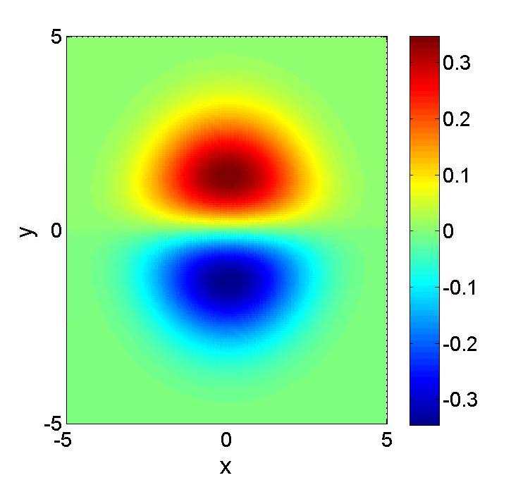
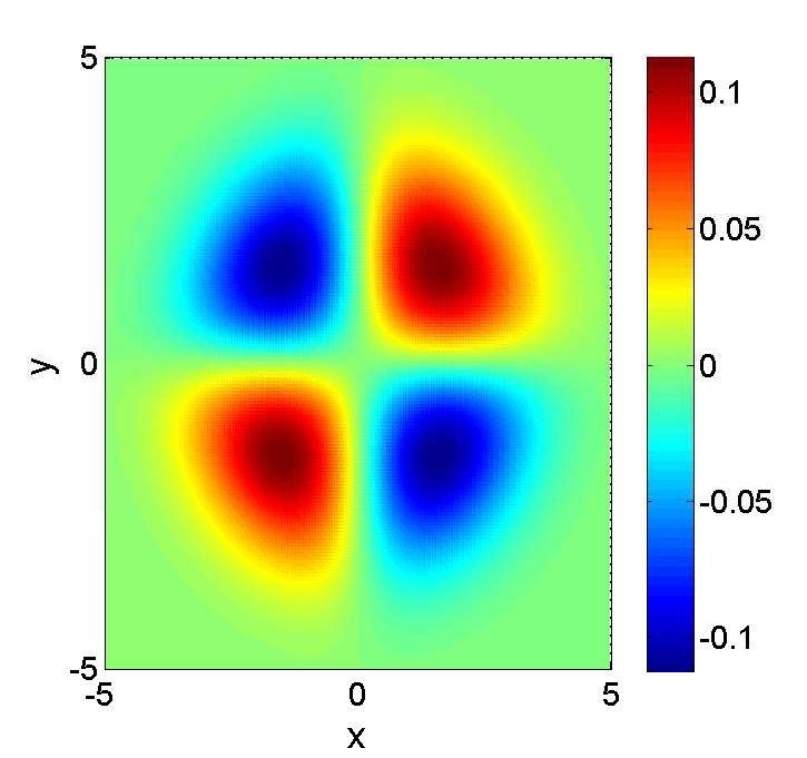
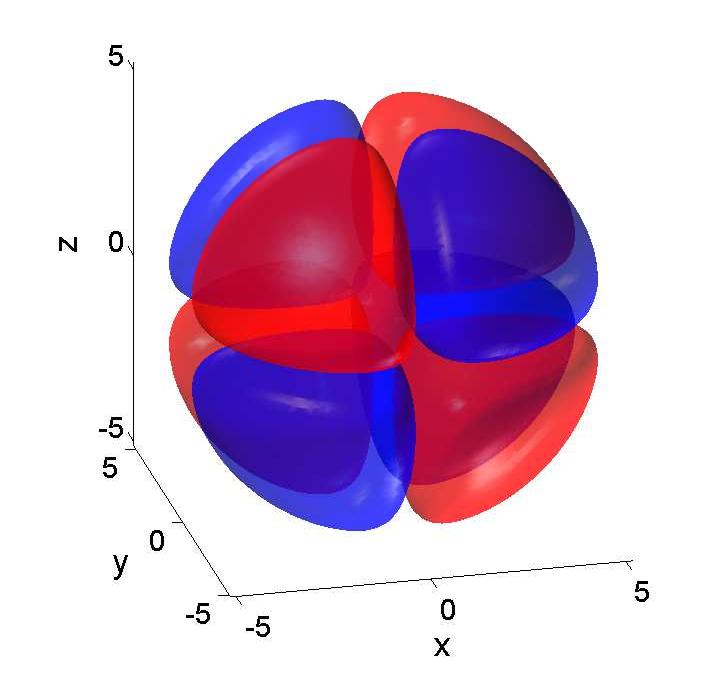
Figure 1: (Color online) Generic examples of numerically found dipole (a) and quadrupole (b) modes in the 2D setting, and of the octupole (c) in 3D. These modes are described by real wave functions $U$ with $\mu=2$, see Eq. (6). In (c), the 3D image of the octupole is displayed by means of red and blue isosurfaces, which correspond, respectively, to $U=+0.01$ and $U=-0.01$.

Numerically found shapes of the 2D dipole ($m=1$) and quadrupole ($m=2$) modes, which are displayed in Figs. 1(a) and (b), suggest that these modes may be approximated, in the simplest form, by a real ansatz,

$$U_{m}(r,\varphi)=V_{\mathrm{2D}}(r)\cos\left(m\varphi\right).$$ (9)

The substitution of this into Eq. (9), and the use of the usual mean-field approximation, $\cos^{3}\left(m\varphi\right)\rightarrow(3/4)\cos\left(m\varphi\right)$, yields the following radial equation:

$$\mu V_{\mathrm{2D}}=-\left(\frac{d^{2}}{dr^{2}}+\frac{1}{r}\frac{d}{dr}-\frac{m^{2}}{r^{2}}\right)V_{\mathrm{2D}}+\frac{3}{4}\exp\left(\frac{r^{2}}{2}\right)V_{\mathrm{2D}}^{3}.$$ (10)

The application of the TFA to Eq. (10) implies neglecting the derivative terms, which yields the simple result:

$$V_{\mathrm{2D}}^{2}(r)=\left\{\begin{array}[]{c}0,~{}r^{2}<\frac{m^{2}}{\mu},\\ \frac{4}{3}\left(\mu-\frac{m^{2}}{r^{2}}\right)\exp\left(-\frac{r^{2}}{2}\right),~{}r^{2}>\frac{m^{2}}{\mu}~{}.\end{array}\right.$$ (11)

This approximation predicts that maxima of the amplitude are located at distance from the origin

$$r_{\mathrm{2D}}^{(\max)}=\sqrt{\frac{|m|}{2\mu}\left(\sqrt{8\mu+m^{2}}+|m|\right)}.$$ (12)

Amplitude maxima of the numerical solutions, found for $\mu=2$, are located at distances $r_{\mathrm{dipole}}^{(\max)}=1.37$, $r_{\mathrm{quadrupole}}^{(\max)}=2.2$, and $r_{\mathrm{octupole}}^{(\max)}=3.46$ from the origin, while the TFA results (12) and (17) (see below) predict, for the same case ($\mu=2$), $r_{\mathrm{dipole}}^{(\max)}=1.13$, $r_{\mathrm{quadrupole}}^{(\max)}=1.8$, and $r_{\mathrm{octupole}}^{(\max)}=2.75$. Naturally, the agreement improves for larger $\mu$, i.e., larger $N$, as the TFA is more accurate for stronger nonlinearity (the increase of $\mu$ from $2$ to $10$ leads to a decrease of the relative difference between the numerical solutions and their TFA counterparts by a factor $\simeq 2$).

Families of the modes are characterized by the norm (total power) as a function of $\mu$. The TFA based on Eq. (11) produces the following dependence:

$$N_{\mathrm{2D}}^{\left(\mathrm{TFA}\right)}(\mu;m)=\frac{2\pi}{3}\int_{m^{2}/\left(2\mu\right)}^{\infty}\left(2\mu-\frac{m^{2}}{\rho}\right)e^{-\rho}d\rho,$$ (13)

where $\rho\equiv r^{2}/2$, and the integral can be easily computed numerically. In the limit of $\mu\rightarrow\infty$, Eq. (13) yields an asymptotically constant slope,

$$\frac{d}{d\mu}N_{\mathrm{2D}}^{\left(\mathrm{TFA}\right)}\left(\mu\rightarrow\infty\right)=\frac{4\pi}{3}.$$ (14)

Dependences (13) for $m=1$ and $m=2$ are displayed in Fig. 2(a), along with their counterparts produced by full numerical solutions of Eq. (7).

In the 3D geometry, the typical shape of the octupoles, displayed in Fig. 1(c), suggests that the corresponding angular structure may be approximated by spherical harmonics with quantum numbers $l=3,m=\pm 2$ LL : $Y_{32}\equiv Y_{3}^{+2}+Y_{3}^{-2}=C\cos\vartheta\sin^{2}\vartheta\cos\left(2\varphi\right)$, where the constant $C$ is not essential here, $\vartheta$ is the second angular coordinate, and $\mathbf{\hat{l}}^{2}Y_{32}=12Y_{32}$. Thus, the ansatz for the octupole is adopted as

$$U(r,\vartheta,\varphi)=V_{\mathrm{3D}}(r)\cos\vartheta\sin^{2}\vartheta\cos\left(2\varphi\right).$$ (15)

For the application of the mean-field approximation to the angular dependence in the cubic term of Eq. (8), $\left[Y_{32}\left(\vartheta,\varphi\right)\right]^{3}$ must be projected back onto $Y_{32}\left(\vartheta,\varphi\right)$, which is done with the help of the standard formula, $\left\langle f(\vartheta)\right|\left|g(\vartheta)\right\rangle=\int_{0}^{\pi}f(\vartheta)g(\vartheta)\left(\sin\vartheta\right)d\vartheta$. The eventual results produced by the 3D version of the TFA are

$$V_{\mathrm{3D}}^{2}(r)\approx\left\{\begin{array}[]{c}0,~{}r^{2}<\frac{12}{\mu},\\ \frac{143}{12}\left(\mu-\frac{12}{r^{2}}\right)\exp\left(-\frac{r^{2}}{2}\right),~{}r^{2}>\frac{12}{\mu}~{}.\end{array}\right.$$ (16)

cf. Eq. (11),

$$r_{\mathrm{3D}}^{(\max)}=\sqrt{\frac{6}{\mu}\left(\sqrt{\frac{2}{3}\mu+1}+1\right)},$$ (17)

cf. Eq. (12), and

$$N_{\mathrm{3D}}^{\left(\mathrm{TFA}\right)}(\mu)=\frac{572\pi}{315}\int_{\sqrt{12/\mu}}^{\infty}\left(\mu r^{2}-12\right)e^{-r^{2}/2}dr,$$ (18)

cf. Eq. (13), with

$$\frac{d}{d\mu}N_{\mathrm{3D}}^{\left(\mathrm{TFA}\right)}\left(\mu\rightarrow\infty\right)=\frac{143}{315}(2\pi)^{3/2},$$ (19)

cf. Eq. (14). The plot produced by Eq. (18) is displayed in Fig. 2(b), along with its counterpart generated by the full numerical solution.

An essential finding revealed by the systematic numerical analysis of the 2D setting is that the increase of $\mu$ (and $N$) leads to destabilization of the 2D dipole mode at a critical point,

$$\mu_{\mathrm{cr}}^{\mathrm{(VAP)}}=1.64,~{}N_{\mathrm{cr}}^{\mathrm{(VAP)}}=1.38,$$ (20)

by a bifurcation, which gives rise to a new mode in the form of a VAP, which will be presented in the next section. Further, careful analysis demonstrates that both 2D quadrupoles and 3D octupoles are, strictly speaking, entirely unstable solutions. Nevertheless, they are robust objects, provided that their norms are relatively small, as the instability is very weak in that case. For the quadrupoles, the simulations reveal that the robustness interval is $\mu<\mu_{\max}\simeq 3$, corresponding to $N<N_{\max}\simeq 1.55$, see Fig. 2(a). In this interval, initially perturbed quadrupoles maintain their shape as long as the simulations were run (with the evolution times measured in many dozens of characteristic dispersion times), exhibiting small-amplitude oscillations between the unperturbed shape and a coexisting stable isotropic VAQ mode (the latter one is presented in detail below). For the octupoles a similarly defined robustness border is located at $\mu_{\max}\simeq 2$, corresponding to a low value of the 3D norm, $N\simeq 0.03$.

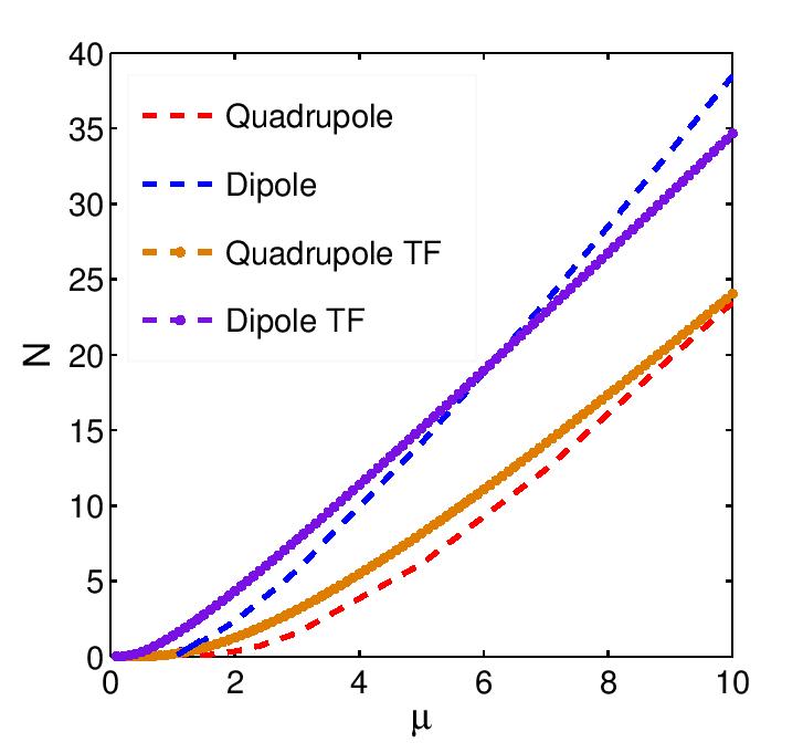
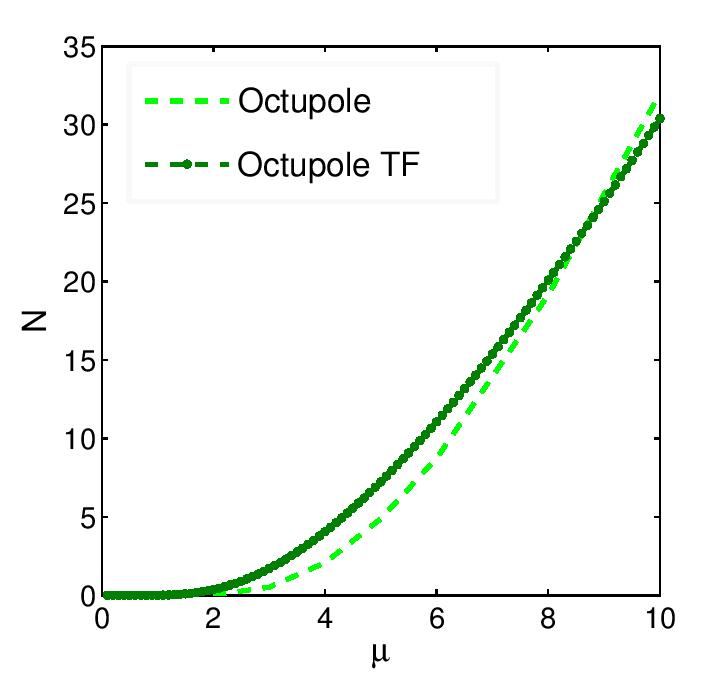
Figure 2: (Color online) Lines labeled “Dipole”, “Quadrupole”, and “Octupole” show, respectively, the 2D and 3D norms, $N$, vs. $\mu$ for these modes, as obtained from numerical computations. The lines marked by “TF” display the predictions for the same dependences produced by the Thomas-Fermi approximation, as per Eqs. (13) and (18). The short solid segment of the $N(\mu)$ curve for the dipole-mode family designates a completely stable subfamily (cf. Fig. 5 below).

The application of the torque to the stable 2D dipole mode, i.e., the multiplication of the respective stationary solution by the phase factor

$$T=\exp\left(ipy\tanh\left(x/x_{0}\right)\right),$$ (21)

with real constants $p$ and $x_{0}$ gyroscope , readily sets it in persistent rotation, thus creating a robust “propeller” mode, cf. Ref. propeller , which preserves the original two-peak shape. The spinning regime is illustrated by a set of snapshots in Fig. 3, where the rotation period is $T=3.9$. Rotation of the dipole was simulated up to $t=100$, amplitude oscillations of the dipole in the course of rotation being limited to $\simeq 2\%$ of its initial value. On the other hand, the application of the torque to the quadrupoles and octupoles does not generate persistently rotating states, in accordance with the above conclusion that these species do not represent fully stable modes.

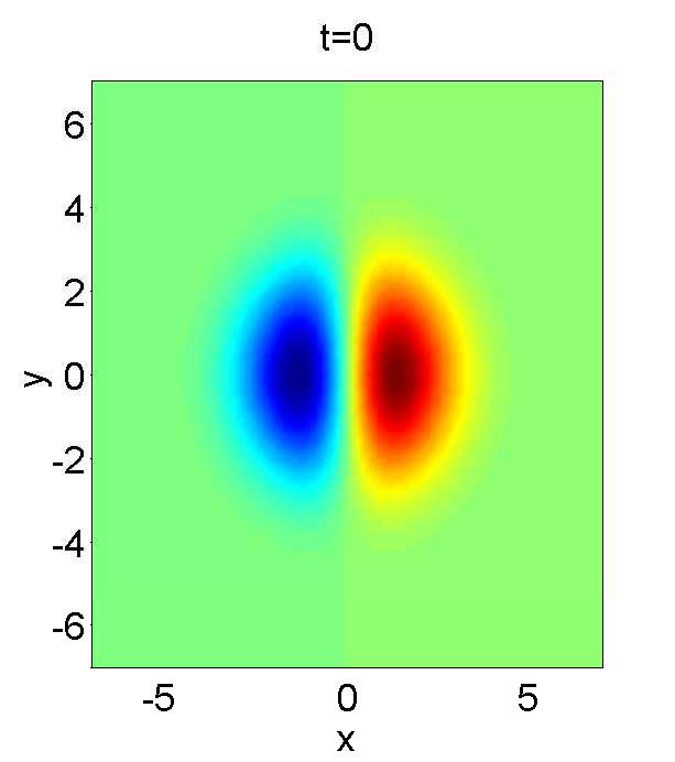
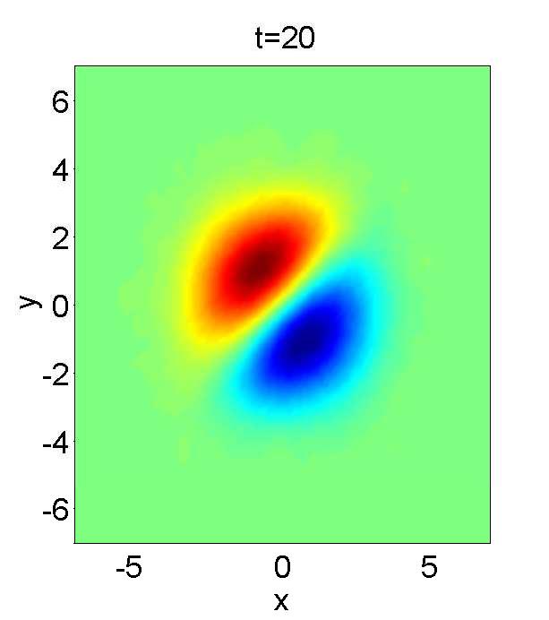
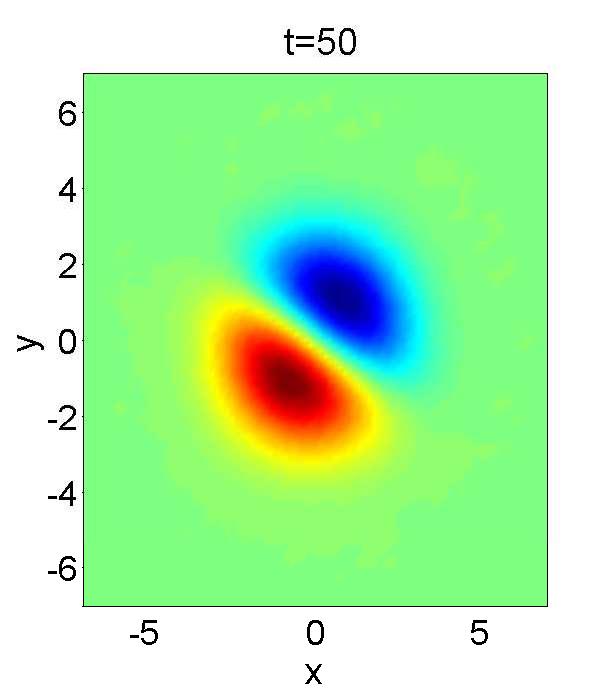
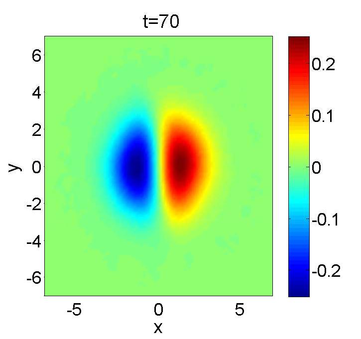
Figure 3: Persistent rotation of a stable dipole with $\mu=1.5$, initiated by the application of a torque, given by Eq. (21) with $p=1$, $x_{0}=10$.

IV Vortex-antivortex pairs (VAPs)

In addition to multipoles, bound pairs of vortices with opposite signs of angular momenta were investigated. A typical example of the VAP and the respective bifurcation diagram are displayed in Figs. 4 and 5, respectively. As seen in panel (a) of Fig. 4, the amplitude profile of the VAP is quite similar to that of the dipole mode, but panel (b) of the same figure demonstrates the phase structure of the stationary VAP, which its real dipole-mode counterpart does not have. It is exactly the phase structure which makes it possible to identify the new mode as the vortex-antivortex bound state.

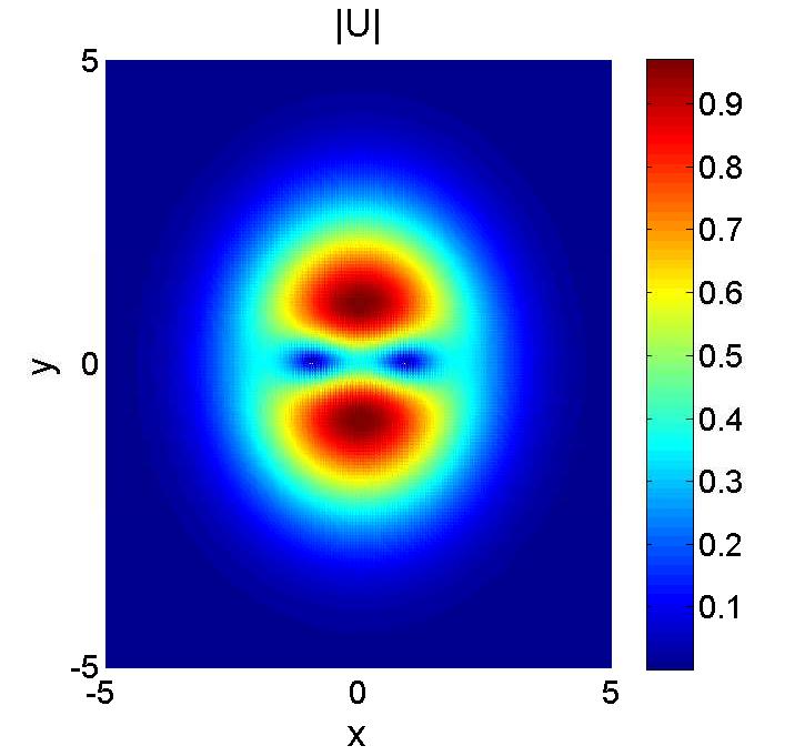
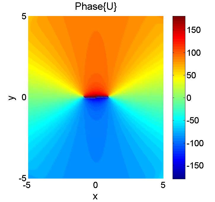
Figure 4: An example of the amplitude and phase profiles of a 2D stable vortex-antivortex pair (VAP), obtained in the numerical form for $\mu=5$ (the corresponding norm is $N=14.78$).  The phase distribution is displayed in degrees.

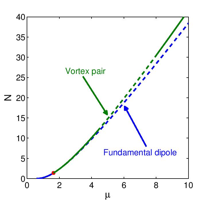
Figure 5: $N(\mu)$ curves for the dipole-mode and vortex–antivortex-pair (VAP) families. Stable and unstable subfamilies are indicated by continuous and dotted lines, respectively. The red dot marks the bifurcation point (20), at which the VAP family branches off from the dipole-mode one.

In accordance with what is said above, the stability of the modes under the consideration was identified by means of systematic simulations of their perturbed evolution. As shown in Fig. 5, the VAP is stable after the bifurcation point, viz., at $1.64<\mu<4.06$, $1.38<N<10.35$, then it is destabilized by oscillatory (in $t$) perturbations in a finite region adjacent to the stability area, $4.06<\mu<8.06$, $10.35<N<30.76$, which is followed by the eventual restabilization of the VAP at $\mu>8.06$, $N>30.76$. Stable VAPs can be easily set in spinning motion, similar to what is shown above for dipoles.

The emergence of the VAPs determines the instability of the dipole modes. In the interval adjacent to the critical point Eq. (20), $1.64<\mu<3$, the dipole features a weak instability, periodically oscillating between its unperturbed shape and the coexisting stable VAP, whose amplitude profile is close to the dipole’s one (not shown in detail here). A similar dynamical regime, featuring remittent shape revivals of a weakly unstable dipole state, was observed in a model with a nonlocal nonlinearity MultipolesNonlocal . At $\mu>3$, the dipole’s instability gets stronger, leading to its spontaneous transformation into a fundamental isotropic state (not shown in detail either).

V Vortex-antivortex quadruplets (VAQs)

Similar to the 2D dipoles, which coexist with VAPs, real stationary 2D quadrupoles coexist with a branch of stable complex solutions for vortex-antivortex bound states in the form of the (isotropic) VAQ, see a typical example of the latter in Fig. 6. However, Fig. 7 demonstrates the difference from the situation for the coexistence of the dipoles and VAPs: the isotropic-VAQ branch emerges at $\mu=0$, rather than branching off from the quadrupole one at a finite value of $\mu$, cf. Fig. 5. Recall that, unlike the dipoles, quadrupole solutions are, strictly speaking, always unstable, hence, indeed, a new stable branch cannot bifurcate from them. As shown in Fig. 7 , the isotropic-VAQ family is stable at $0<\mu<5.74$ (which corresponds to $0<N<11.06$). At $\mu>5.74$ ($N>11.06$), these modes become unstable against oscillatory perturbations, eventually evolving into the isotropic ground state (not shown here in detail).

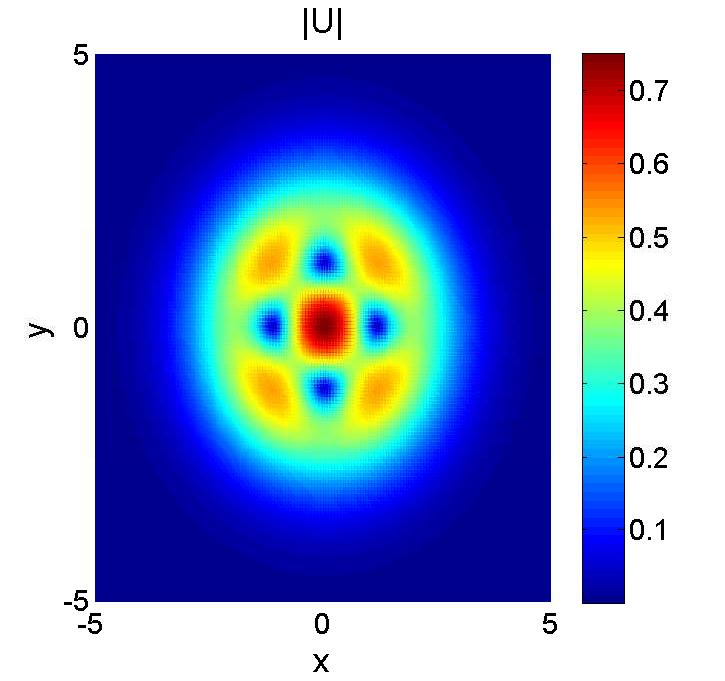
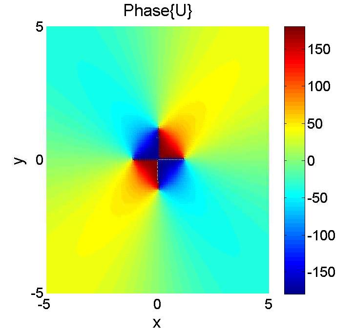
Figure 6: The amplitude (a) and phase (b) profiles of a stable isotropic vortex-antovortex quadruplet (VAQ) at $\mu=5$ and $N=8.12$.

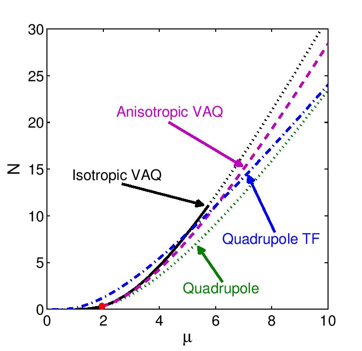
Figure 7: Juxtaposed $N(\mu)$ curves for the (fully unstable) quadrupoles, as produced by the numerical results and by the Thomas-Fermi approximation (“TF”) [these two curves are the same as in Fig. 2(a)], and for the (partly stable) isotropic and (fully unstable) anisotropic vortex-antivortex quadruplets (VAQs). As usual, stable and unstable families of solutions are indicated by solid and dotted lines, respectively. The dashed-dotted and dashed lines refer, severally, to the Thomas-Fermi approximation for the quadrupoles and the anisotropic VAQs. The bifurcation point (22), at which the anisotropic-VAQ branch splits off from its isotropic counterpart, is marked by the red dot.

Further, a new branch, of anisotropic VAQs (AVAQs), bifurcates from the family of their isotropic counterparts at

$$\mu_{\mathrm{cr}}^{(\mathrm{aniso})}=1.96,~{}N_{\mathrm{cr}}^{(\mathrm{aniso})}=0.33.$$ (22)

A typical example of an AVAQ mode is displayed in Fig. 8. The analysis demonstrates that this solution is always unstable [this fact explains why the bifurcation occurring at point (22) does not destabilize the branch of the isotropic VAQs]. Specifically, from the bifurcation point (22) up to $\mu=12.54$ ($N=40.77$), a perturbed AVAQ solution starts spinning motion, with an angular velocity determined by the initial perturbation, see an example in Fig. 9 (in this case, the conservation of the angular momentum is provided by the recoil effect of small-amplitude waves emitted by the perturbed AVAQ, which are not visible in Fig. 9). Eventually, the unstable spinning AVAQ transforms not into the isotropic ground state, which is typical for other species of unstable modes which were mentioned above, but, instead, into a stably rotating VAP. In several cases that were examined, this transition occurred before the AVAQ would complete half a cycle of its rotation. Finally, at $\mu>12.54$ ($N>40.77$), the AVAQ immediately transforms into a rotating VAP, without going through the intermediate spinning stage (not shown here in detail).

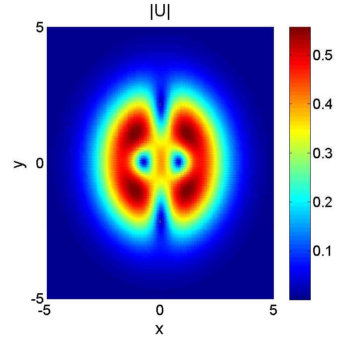
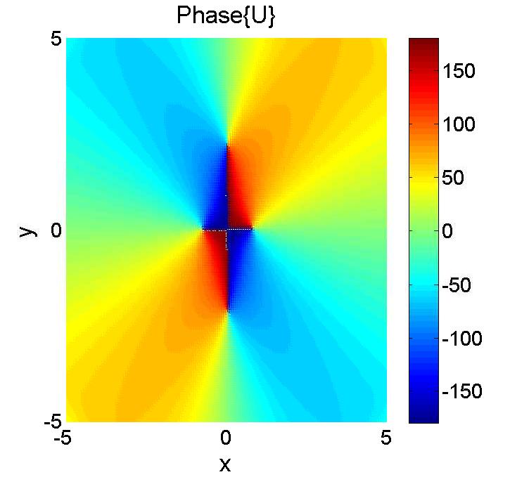
Figure 8: The same as in Fig. 6, but for an unstable anisotropic VAQ, with $\mu=5$, $N=7.40$.

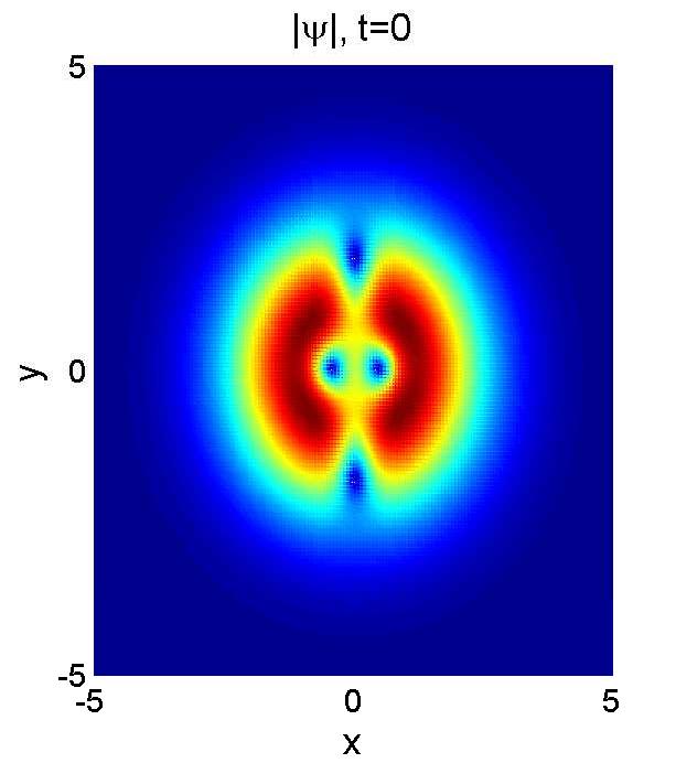
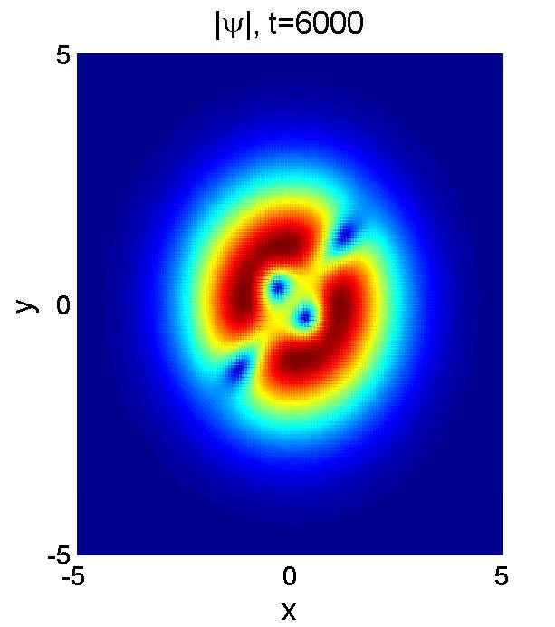
Figure 9: The transient rotation of the unstable AVAQ, with $\mu=12$, $N=38.08$, prior to its spontaneous transformation into a stable vortex-antivortex pair.

VI Conclusion

The recently introduced class of optical and matter-wave models, with the strength of the self-repulsive cubic nonlinearity growing from the center to periphery, gives rise to a large variety of completely stable complex 2D and 3D self-trapped states (solitons), which do not exist or are strongly unstable in other physical settings. Here we have demonstrated that, together with previously found states, the same models support several other species of 2D and 3D solitons which are not available (in a stable form) in other systems either. These are 2D dipoles and quadrupoles and 3D octupoles, as well as VAPs (vortex-antivortex pairs) and isotropic or anisotropic VAQs (vortex-antivortex quadruplets). The modes found here are stable or weakly unstable, surviving for a long time (over a long propagation distance), which makes them physically relevant objects. In addition to quiescent states, persistently spinning dipoles have been found too. The results, which were obtained by means of numerical methods and analytically, using the TFA (Thomas-Fermi approximation), demonstrate the potential of the settings with the spatially growing strength of the self-repulsion for the creation of a great variety of complex stable  multidimensional modes.

Natural extensions of the present analysis may be additional analysis of the 3D setting (in particular, for 3D dipoles and quadrupoles), and its development for two-component systems, in which the multitude of nontrivial self-trapped states may be further expanded, as suggested, e.g., by results for the two-component system in 1D two-component .

- (1) Kivshar Y S and Agrawal G P 2003 Optical Solitons: From Fibers to Photonic Crystals (Academic Press: San Diego).
- (2) Etrich C, Lederer F, Malomed B A, Peschel T, and Peschel U 2000 Prog. Opt. 41, 483-568 (2000); Buryak A V, Di Trapani P, Skryabin D V, and Trillo S 2002 Phys. Rep. 370 63.
- (3) Malomed B A, Mihalache D, Wise F, and Torner L 2005 J. Opt. B: Quantum Semiclass. Opt. 7 R53; Fleischer J W, Bartal G, Cohen O, Schwartz T, Manela O, Freedman B, Segev M, Buljan H, and Efremidis N K 2005 Opt. Express 13, 1780; Desyatnikov A S, Kivshar Y S, and Torner L 2005 Prog. Opt. 47, 291; Mihalache D 2010 J. Optoelectron. Adv. Mater. 12 12; Chen Z, Segev M, and Christodoulides D N 2012 Rep. Prog. Phys. 75 086401.
- (4) Kartashov Y V, Malomed B A, and Torner L 2011 Rev. Mod. Phys. 83 247.
- (5) Kasamatsu K, Tsubota M, and Ueda M 2005 Int. J. Mod. Phys. B 19 1835; Fetter A L 2009 Rev. Mod. Phys. 81 647.
- (6) Alkofer R, Reinhardt H, and Weigel H 1996 Phys. Rep. 265 139; Bender M, Heenen P H, and Reinhard P G 2003 Rev. Mod. Phys. 75 121; Sakai T and Sugimoto S 2005 Prog. Theor. Phys. 113 843 (2005).
- (7) Radu E and Volkov M S 2008 Phys. Rep. 468 101.
- (8) Yang J 2010 Nonlinear Waves in Integrable and Nonintegrable Systems (SIAM: Philadelphia).
- (9) Bergé L 1998 Phys. Rep. 303 259 (1998); Kuznetsov E A and Dias F 2011 ibid. 507 43.
- (10) Królikowski W, Ostrovskaya E A, Weilnau C, Geisser M, McCarthy G, Kivshar Yu S, Denz C and Luther-Davies B 2000 Phys. Rev. Lett. 85 1424; Desyatnikov A S, Kivshar Y S, Motzek K, Kaiser F, Weilnau C and Denz C 2002 Opt. Lett. 27 634; Kartashov Y V, Ferrando A and Garcia-March M-A 2007 ibid. 32 2155; Izdebskaya Y V, Desyatnikov A S, Assanto G and Kivshar Y S 2011 Opt. Express 19 21457.
- (11) Lashkin V M 2007 Phys. Rev. A 75 043607; Abdullaev F Kh, Kartashov Y V, Konotop V V and Zezyulin D A 2011 ibid. 83 041805(R); Lobanov V E, Kartashov Y V and Konotop V V 2014 Phys. Rev. Lett. 112 180403.
- (12) Yang J, Makasyuk I, Bezryadina A and Chen Z 2004 Opt. Lett. 29 1662; Kartashov Y V, Egorov A A, Vysloukh V A and Torner L 2004 J. Opt. B: Quant. Semiclass. Opt. 6 444; Kartashov Y V, Carretero-González R, Malomed B A, Vysloukh V A and Torner L 2005 Opt. Express 13 10703.
- (13) Yang J and Pelinovsky D E 2003 Phys. Rev. E 67 016608.
- (14) Carmon T, Uzdin R, Pigier C, Musslimani Z H, Segev M, and Nepomnyashchy A 2001Phys. Rev. Lett. 87 143901.
- (15) Lopez-Aguago S, Desyatnikov A S, Kivshar Y S, Skupin S, Królikowski W and Bang O 2006 Opt. Lett. 31 1100; Zhong W, Yi L, Xie R, Belić M, and Chen G 2008 J. Phys. B 41 025402.
- (16) Edmundson D E and Enns R H 1992 Opt. Lett. 17 586; Edmundson D E and Enns R H 1993 ibid. 18 1609 (1993); Enns R H and Rangnekar S S 1992 Phys. Rev. A 45 3354; Enns R H and Rangnekar S S 1993 Phys. Rev. E 48 3998.
- (17) Duree G C, Shultz J L , Salamo G J , Segev M, Yariv A, Crosignani B, Di Porto P, Sharp E J, and Neurgaonkar R R 1993 Phys. Rev. Lett. 71 533.
- (18) Tikhonenko V, Christou J, and Luther-Davies B 1995 J. Opt. Soc. Am. B 12 2046.
- (19) Quiroga-Teixeiro M and Michinel H J. Opt. Soc. Am. B 1997 14 2004; Mihalache D, Mazilu D, Crasovan L-C, Towers I, Buryak A V, Malomed B A, Torner L, Torres J P and Lederer F 2002 Phys. Rev. Lett. 88 073902; Driben R, Malomed B A, Gubeskys A, and Zyss J 2007 Phys. Rev. E 76 066604; Wang Z, Cherkasskii M, Kalinikos B A, Carr L D, and Wu M 2014 New J. Phys. 16, 053048; Shen M, Wu D, Zhao H, and Li B 2014 J. Phys. B: At. Mol. Opt. Phys. 47 255401; Danshita I, Yamamoto D, and Kato Y 2015 Phys. Rev. A 91 013630.
- (20) Bang O, Kivshar Y S, and Buryak A V 1997 Opt. Lett. 22, 1680; Bang O, Kivshar Y S, Buryak A V, de Rossi A, and Trillo S 1998 Phys. Rev. E 58 5057; Liu X, Qian L J, Wise F W 1999 Phys. Rev. Lett. 82, 4631; Liu X, Beckwitt K, Wise F W 2000 Phys. Rev. E 62, 1328; Mihalache D, Mazilu D, Crasovan L-C, Towers I, Malomed B A, Buryak A V, Torner L, and Lederer F 2002 Phys. Rev. E 66 016613.
- (21) Królikowski W, Bang O, Nikolov N I, Neshev D, Wyller J, Rasmussen J J, and Edmundson D 2004 J. Opt. B: Quantum Semiclass. Opt. 6 S288-S294; Maucher F, Henkel N, Saffman M, Królikowski W, Skupin S, and Pohl T 2011, Phys. Rev. Lett. 106 170401; Bang O, Królikowski W, Wyller J, Rasmussen J J, Phys. Rev. E 66 046619 (2002).
- (22) Bang O, Christiansen P L, If F, Rasmussen K Ø, and Gaididei Y B 1994, Phys. Rev. E 49 4627.
- (23) Bang O, Edmundson D, and Królikowski W, 1999 Phys. Rev. Lett. 83 5479.
- (24) Wyller J, Królikowski W, Bang O, and Rasmussen J J 2002, Phys. Rev. E 66 066615.
- (25) Falção-Filho E L, de Araújo C B, Boudebs G, Leblond H and Skarka V 2013 Phys. Rev. Lett. 110 013901.
- (26) Reyna A S, Jorge K C, and de Araújo C B 2014 Phys. Rev. A 90, 063835.
- (27) Towers I and Malomed B A 2002 J. Opt. Soc. Am. B 19 537; Abdullaev F Kh Caputo J G, Kraenkel R A, and Malomed B A 2003 Phys. Rev. A 67 013605; Saito H and Ueda M 2003 Phys. Rev. Lett. 90 040403; Montesinos G D, Pérez-García V M, and Torres P J 2004 Physica D 191 193; Matuszewski M, Infeld E, Malomed B A and Trippenbach M 2005 Phys. Rev. Lett. 95 050403; Itin A, Morishita T, and Watanabe S 2006 Phys. Rev. A 74 033613.
- (28) Efremidis N K, Sears S, Christodoulides D N, Fleischer J W, and Segev M 2002 Phys. Rev. E 66, 046602; Baizakov B B, Malomed B A and Salerno M 2003 Europhys. Lett. 63, 642-648; Yang J and Musslimani Z H 2003 Opt. Lett. 28, 2094; Baizakov B B, Malomed B A and Salerno M 2004 Phys. Rev. A 70 053613; Mihalache D, Mazilu D, Lederer F, Kartashov Y V, Crasovan L-C and Torner L 2004 Phys. Rev. E 70 055603; Driben R and Malomed B A 2008 Eur. Phys. J. D 50 317; Zhong W-P, Belić M and Huang T 2010 Phys. Rev. A 82 033834; Panagiotopoulos P, Couairon A, Efremidis N K, Papazoglou D G and Tzortzakis S 2011 Opt. Express 19 10057 Li H-j, Wu Y-p, Hang C and Huang G 2012 Phys. Rev. A 86 043829.
- (29) Fleischer J W, Segev M, Efremidis N K, and Christodoulides D N 2003 Nature 422 147; Fleischer J W , Carmon T, Segev M, Efremidis N K, and Christodoulides D N 2003 Phys. Rev. Lett. 90 023902; Efremidis N K, Hudock J, Christodoulides D N, Fleischer J W, Cohen O, and Segev M 2003 ibid. 91 213905; Neshev D, Alexander T J, Ostrovskaya E A, Kivshar Y S, Martin H, Makasyuk I, and Chen Z 2004 ibid. 92 123903; Fleischer J W, Bartal G, Cohen O, Manela O, Segev M, Hudock J, and Christodoulides D N 2004 ibid. 92 123904; Fischer R, Träger D, Neshev D N, Sukhorukov A A, Królikowski W, Denz C, and Kivshar Y S 2006 ibid. 96 023905.
- (30) Borovkova O V, Kartashov Y V, Malomed B A, and Torner L 2011 Opt. Lett. 36 3088-3090; Borovkova O V, Kartashov Y V, Torner L, and Malomed B A 2011 Phys. Rev. E 84 035602 (R).
- (31) Tian Q, Wu L, Zhang Y, and Zhang J-F 2013 Phys. Rev. E 85, 056603 (2012); Wu Y, Xie Q, Zhong H, Wen L, and Hai W 2013 Phys. Rev. A 87, 055801; Xie Q, Wang L, Wang Y, Shen Z, and Fu J 2014 Phys. Rev. E 90 063204.
- (32) Driben R, Kartashov Y V, Malomed B A, Meier T, and Torner L 2014 Phys. Rev. Lett. 112 020404.
- (33) Driben R, Kartashov Y V, Malomed B A, Meier, T and Torner L 2014 New Journal of Physics 16 063035.
- (34) Kartashov Y V, Malomed B A, Shnir Y, and Torner L (2014) Phys. Rev. Lett. 113 264101.
- (35) Piette B M A G, Schroers B J, and Zakrzewski W J 1995, Zeitschr. Phys. C: Particles and Fields 65 165.
- (36) Driben R, Meier T, and Malomed B A 2015 Scientific Reports 5 9420.
- (37) Hukriede J, Runde D, and Kip D 2003 J. Phys. D 36 R1.
- (38) Yamazaki R, Taie S, Sugawa S, and Takahashi Y 2010 Phys. Rev. Lett. 105 050405.
- (39) Henderson K, Ryu C, MacCormick C, and Boshier M G 2009 New J. Phys. 11 043030.
- (40) Ghanbari H S , Kieu T D, Sidorov A, and Hannaford P 2006 J. Phys. B: At. Mol. Opt. Phys. 39 847; Romero-Isart O, Navau C, Sanchez A, Zoller P, and Cirac J I 2013 Phys. Rev. Lett. 111 145304; Ghanbari S, Abdalrahman A, Sidorov A, and Hannaford P 2014 J. Phys. B: At. Mol. Opt. Phys. 47 115301 (2014); Jose S, Surendran P, Wang Y, Herrera I, Krzemien L, Whitlock S, McLean R, Sidorov A, and Hannaford P 2014 Phys. Rev. A 89 051602.
- (41) Kevrekidis P G, Malomed B A, Saxena A, Bishop A R, and Frantzeskakis D J (2015) Phys. Rev. E 91 043201 (2015).
- (42) Li Y, Liu J, Pang W, and Malomed B A 2013 Phys. Rev. A 88 053630.
- (43) Molina-Terriza G, Torres J P and Torner L 2007 Nature Phys. 3 305-310.
- (44) Chiofalo M L, Succi S and Tosi M P 2000 Phys. Rev. E 62 7428.
- (45) Chen J C and Jüngling S 1994 Optical and Quantum Electronics 26 S199.
- (46) Lakoba T I and Yang J Journal of Comput. Phys. 2007 226 1668.
- (47) Landau L D and Lifshitz E M, Quantum Mechanics (Moscow: Nauka Publishers, 1974).
- (48) Kartashov Y V, Vysloukh V A, Torner L, and Malomed B A 2011 Opt. Lett. 36 4587 (2011).