Abstract

We consider nucleon-decay-like signatures of the hylogenesis, a variant of the antibaryonic dark matter model. For the interaction between visible and dark matter sectors through the neutron portal, we calculate the rates of dark matter scatterings off neutron which mimic neutron-decay processes $n\to\nu\gamma$ and $n\to\nu e^{+}e^{-}$ with richer kinematics. We obtain bounds on the model parameters from nonobservation of the neutron decays by applying the kinematical cuts adopted in the experimental analyses. The bounds are generally (much) weaker than those coming from the recently performed study of events with a single jet of high transverse momentum and missing energy observed at the LHC. Then we suggest several new nucleon-decay like processes with two mesons in the final state and estimate (accounting for the LHC constraints) the lower limits on the nucleon lifetime with respect to these channels. The obtained values appear to be promising for probing the antibaryonic dark matter at future underground experiments like HyperK and DUNE.

1 Introduction

Given a variety of spatial scales and cosmological epochs associated with dark matter phenomena, their natural explanation seems in introducing a new neutral particle, stable at cosmological time-scales. Many extensions of the Standard Model of particle physics (SM) suggest suitable dark matter candidates with masses ranging from $10^{-23}$ eV (oscillating scalar field, see e.g. [18]) to $10^{16}$ GeV (superheavy dark matter, see e.g. [13]). Dark matter particles must be produced in the early Universe at a stage before matter-radiation equality. Most mechanisms exploited for this purpose work properly (for a review see [2]) but treat the (order-of-magnitude) equality of dark matter and visible matter contributions to the present energy density of Universe,

$$\rho_{\text{DM},0}\sim\rho_{\text{B},0}\,,$$ (1)

as an accidental coincidence.

Yet it may be a hint towards a common origin of both cosmological problems, dark matter phenomena and matter-antimatter asymmetry of the Universe. There are models addressing this issue. In particular, an elegant approach is provided by models of antibaryonic dark matter, where dark matter particles carry (anti)baryonic charge. The idea is that the total baryonic charge of the Universe is zero, but it is redistributed between visible sector (positive baryonic charge) and dark sector (negative charge of the same amount). Both dark and visible matter emerge during the same process at some stage in the early Universe making a connection between the two components, so that the coincidence (1) may be understood.

Similar to the visible sector, the dark sector is asymmetric, being populated solely with particles of negative baryonic charge. The models of this type are called asymmetric dark matter, for a review see [21]. They exhibit quite specific phenomenology. As a rule, no dark matter pair annihilation is expected in galaxies or inside the Sun (see, however, [15, 3]). Instead, the antibaryonic dark matter particle may annihilate with nucleon, mimicking proton/neutron disappearance or decay.

A remarkable example of the antibaryonic dark matter model is provided by hylogenesis [9]. To the SM particle content at low energies the model adds a complex scalar $\Phi$ and Dirac spinor $\Psi$, together forming dark matter components, and also two heavy fermions $X_{a}$, $a=1,2$, playing the role of messengers between the visible and dark sectors. The interaction terms read

$${\cal L}=-\frac{\lambda_{a}^{ijk}}{\Lambda^{2}}\,\overline{X_{a}}\,\frac{1+\gamma_{5}}{2}\,d^{i}\cdot\overline{u^{j\,C}}\,\frac{1+\gamma_{5}}{2}\,d^{k}+\zeta_{a}\overline{X_{a}}\Psi^{C}\Phi^{*}+\text{h.c.}\,,$$ (2)

with $i,j,k$ running over the SM three generations, $d^{i}$ and $u^{j}$ denote down-type and up-type quarks, superscript $C$ refers to charge conjugation; $\lambda_{a}^{ijk}$ and $\zeta_{a}$ are dimensionless coupling constants, $\Lambda$ stands for the scale of new physics which completes the model to a renormalizable theory (for a particular variant of high-energy completion within a supersymmetric framework see [6]).

The new fields carry baryonic charge, so that $B(X_{a})=1$ and $B(\Psi)=B(\Phi)=-1/2$. Coupling constants $\lambda_{a}^{ijk}$ and $\zeta_{a}$ are, in general, complex numbers, providing the model with charge ($C$) and charge-parity ($CP$) violation required for the successful dynamical generation of the baryon asymmetry. The latter is produced in the early Universe via $CP$-violating decays of nonrelativistic messengers $X_{a}$ in a way very similar to what happens in the standard leptogenesis with heavy sterile neutrinos [12]. Since the baryon number is conserved by interactions (2), in the same process the dark sector ($\Psi$, $\Phi$) becomes asymmetric, collecting the negative baryonic charge produced in the $CP$-violating decays of nonrelativistic fermions $X_{a}$. Later in the Universe, baryons and antibaryons of the visible sector annihilate, leaving the net baryonic charge, which is accumulated at present mostly in hydrogen and helium. A similar process happens in the dark sector, and the antibaryonic charge of the same amount is distributed between fermions $\Psi$ and bosons $\Phi$. This may be characterized by a ratio of their present number densities,

$$\eta\equiv\frac{n_{\Phi\,,0}}{n_{\Psi\,,0}}\,.$$ (3)

Proton and both dark matter particles, $\Psi$ and $\Phi$, are stable, if their masses obey the kinematical constraints

$$\left|M_{\Psi}-M_{\Phi}\right|<M_{p}+m_{e}<M_{\Psi}+M_{\Phi}\,,$$ (4)

where $M_{p}$ and $m_{e}$ stand for proton and electron masses. Total baryon number conservation implies a simple relation between dark matter and visible baryon number densities

$$n_{B}=\frac{n_{\Psi}+n_{\Phi}}{2}\,.$$ (5)

For the present dark matter energy density, one can write

$$\rho_{DM,0}=M_{\Psi}\,n_{\Psi}+M_{\Phi}\,n_{\Phi}\,.$$ (6)

Without any asymmetry between the two dark matter components, i.e., when $\eta=1$, we obtain from (6) and (5)

$$\rho_{DM,0}=\frac{M_{\Psi}+M_{\Phi}}{M_{p}}\,\rho_{B,0}\,,$$ (7)

which for the observed property (1) settles the dark matter mass scale in the GeV-range. Then, for the present cosmological estimates of $\rho_{B,0}$ and $\rho_{DM,0}$ [20], the sum of the dark matter particle masses are fixed by eq. (7), while the kinematical constraint (4) confines the individual masses inside the interval

$$1.7\,\text{GeV}\lesssim M_{\Psi}\,,\,M_{\Phi}\lesssim 2.9\,\text{GeV}\,.$$ (8)

With asymmetry between $\Psi$ and $\Phi$ populations, $\eta\neq 1$, the relation (7) is replaced with

$$\rho_{DM,0}=\frac{2(M_{\Psi}+\eta\,M_{\Phi})}{(1+\eta)M_{p}}\,\rho_{B,0}\,.$$ (9)

The interaction with quarks in (2) can be used to probe the model at colliders [10, 11]. Heavy fermions $X_{a}$ can be directly produced or virtually contribute to dark matter production. This model provides the following signatures for the LHC experiments (depending on the quark structure in (2)): (i) missing energy and either a jet with high transverse momentum $p_{T}$ [10, 11] or a heavy quark ($t,b,$ or $c$) with high $p_{T}$ [11]; (ii) a jet (or a heavy quark) with high $p_{T}$ and a peak in the invariant mass of three jets whose momenta compensate high $p_{T}$ [11]. The performed analysis of LHC events with a high-$p_{T}$ jet and missing energy has allowed us to constrain the model parameter space pushing the new physics up to TeV scale [11].

Another very pronounced signature of the model  [9] is an induced nucleon decay (IND) [10]. The dark matter particle scattering off a nucleon (through the exchange of virtual fermions $X_{a}$) flips its type, $\Psi\leftrightarrow\Phi$, and destroys the nucleon. The kinematical constraint (4) obviously forbids the traceless disappearance of the nucleon, i.e., a process like $\Phi+n\to\Psi$. Some additional particles must emerge in the final state yielding a signature of the induced nucleon decay. These processes involving an additional single meson in the final state have been analyzed [9, 10, 6] for a set of quark operators entering (2) and a number of final states. While the scattering mimics the nucleon decay, the kinematics of particles in the final state is different, which prevents us from direct use of the limits on the proton/neutron lifetimes to constrain the model parameter space. However, by adjusting properly the kinematical cuts, the corresponding analysis has been performed [6, 10]. In particular, for $X_{a}$ couplings to the $uds$ operator in (2), the results of nucleon decay searches raise the mass of heavy fermion $X_{a}$ and the scale of new physics $\Lambda$ up to the TeV scale [9, 10, 6].

In this paper we analyze several new modes of the induced nucleon decays via a neutron portal, represented by $dud$ operator in (2). The paper is organized as follows. In Sec. 2 we derive the low energy effective lagrangian describing the dark matter scattering off a neutron and give the relation between the scattering cross section and the nucleon lifetime with respect to decay into a given final state. In Sec. 3 we consider $2\to 2$ scattering processes $\Psi(\Phi)+n\to\Phi(\Psi)+\gamma$, which mimic neutron decay $n\to\nu\gamma$, and, imposing the cuts adopted in the experimental search for this decay mode [5, 19], we constrain the model parameter space. These constraints turn out to be (much) weaker than those following from the LHC [11], so finally we obtain a lower estimate of the neutron lifetime in this model based on the limits from the LHC. In a similar way, we investigate the scattering $\Psi(\Phi)+n\to\Phi(\Psi)+e^{+}\,e^{-}$ in Sec. 4. We study the induced nucleon decays into two light mesons ($\pi$, $K$, $\eta$ in various possible combinations) in Sec. 5 and (based on the LHC bounds [11]) predict the shortest lifetimes at the level of $10^{32}-10^{33}$ yr expected for these modes within hylogenesis. The obtained numbers are quite promising and allow the processes to be tested with the next generation underground facilities like HyperK [16, 1] and DUNE [17]. We expect that these channels apart from the dominant single-meson-induced nucleon decays would be helpful to discriminate between different models predicting processes with baryon number violation and corner an interesting region in the parameter space of the hylogenesis scenario if a signal of nucleon-decay-type is found in future. We conclude in Sec. 6.

2 Low-energy effective lagrangian and nucleon lifetime

The coupling terms in eq. (2) relevant for low-energy phenomenology of the neutron portal read

$${\cal L}=-\frac{\lambda_{a}^{dud}}{\Lambda^{2}}\,\overline{X_{a}}\,\frac{1+\gamma_{5}}{2}\,d\cdot\overline{u^{C}}\,\frac{1+\gamma_{5}}{2}\,d+\zeta_{a}\overline{X_{a}}\Psi^{C}\Phi^{*}+\text{h.c.}\,.$$ (10)

Hereafter we are interested in processes with typical energies much below the mass scale of the heavy fermions $X_{a}$. The exchange of virtual $X_{a}$ between the visible sector and dark sector fields entering (10) yields the following contact interaction

$${\cal L}=-\frac{\sum_{a=1}^{2}\frac{\lambda_{a}^{dud}\,\zeta_{a}^{*}}{M_{X_{a}}}}{\Lambda^{2}}\,\Phi\,\overline{\Psi^{C}}\frac{1+\gamma_{5}}{2}\,d\cdot\overline{u^{C}}\,\frac{1+\gamma_{5}}{2}\,d+\text{h.c.}\,.$$ (11)

For further analysis it is convenient to introduce variables $M_{X}$ and $y$ by relations

$$\frac{y}{M_{X}}\equiv\sum_{a=1}^{2}\frac{\lambda_{a}^{dud}\,\zeta_{a}^{*}}{M_{X_{a}}}\,,$$ (12)

so that $M_{X}$ (somewhat vaguely) indicates the heavy fermion scale, while dimensionless parameter $y$ reflects the coupling strength. The physical meaning of $M_{X}$ is the energy scale below which the effective interaction (11) can be safely exploited instead of (10). Since not $y$ and $M_{X}$ individually but only their ratio (12) enters all the formulas below, there is an ambiguity in the definition of $y$ and $M_{X}$ related to the change of the variables. However, it has no impact on the physical observables.

Further, the GeV scale of dark matter masses (8) and smallness of the expected velocity of galactic dark matter particles allow us to describe the dark matter scattering off nucleons in terms of baryons and mesons rather than quarks and gluons. In this approximation, the lagrangian (11) with replacement (12) transforms into Yukawa-type interaction

$${\cal L}=-\frac{y\,\beta}{\Lambda^{2}\,M_{X}}\,\Phi\,\overline{\Psi^{C}}\frac{1+\gamma_{5}}{2}\,n+\text{h.c.}\,,$$ (13)

which we use below to calculate the scattering rates; $n$ denotes the neutron field and the parameter $\beta=0.012$ GeV³ is related to the QCD scale [8].

The cross sections of dark matter scatterings off nucleon $N$, $\sigma_{\Psi N\to\dots}$ and $\sigma_{\Phi N\to\dots}$, are related to the total nucleon lifetime with respect to a particular IND process $\tau_{N\to\dots}$ as follows

$$\tau_{N\to\dots}=\frac{1}{n_{\Psi}\,v\sigma_{\Psi N\to\dots}+n_{\Phi}\,v\sigma_{\Phi N\to\dots}}\,,$$ (14)

where $v$ is the dark matter particle velocity in the laboratory frame where nucleons are at rest. In fact, since the scatterings we discuss happen in $s$-wave, the cross sections are inversely proportional to $v$, and the lifetime (14) does not depend on its value.

3 Scattering processes $\Psi(\Phi)\,n\to\Phi(\Psi)\,\gamma$

We start our study with a simple $2\to 2$ scattering with dark matter particles annihilating a neutron into dark matter particle of another type and a photon. Let $p_{\Psi}$, $p_{n}$ and $q$ be the 4-momentum of $\Psi$, neutron $n$, and the outgoing photon $\gamma$, being real for $\Psi\,n\to\Phi\,\gamma$, and hence $q^{2}=0$ (or virtual for $\Psi\,n\to\Phi\,e^{+}e^{-}$, which we consider in Sec. 4). The process is proceeded due to the Yukawa interaction (13) and the neutron dipole moment

$${\cal L}=\frac{ie}{2M_{n}}\,\bar{n}\sigma^{\mu\nu}q_{\nu}F_{2}(q^{2})nA_{\mu}\;,$$ (15)

where $\epsilon_{\mu}(q)$ is photon polarization 4-vector and for the Pauli (magnetic) form factor we utilize the dipole parametrization $F_{2}(q^{2})=-1.91/(1+q^{2}r_{M}^{2}/12)^{2}$ with magnetic radius $r_{M}=0.86$ fm [20].

The dark matter particle scatters off the neutron by means of virtual neutron exchange. The matrix element of the process reads

$$\frac{iey\beta}{2M_{n}\,\Lambda^{2}}\frac{F_{2}(q^{2})}{M_{X}}\,\overline{\Psi^{C}}(p_{\Psi})\frac{1+\gamma_{5}}{2}\frac{\hat{p}-M_{n}}{p^{2}-M_{n}^{2}}\sigma^{\mu\nu}q_{\nu}n(p_{n})\epsilon_{\mu}(q)\Phi,$$

where $p=q-p_{n}$ is the 4-momentum of the virtual neutron, and $n(p_{n}),\Psi(p_{\Psi}),\Phi$ are wave functions of the neutron, $\Psi$ and $\Phi$ particles, respectively. In the laboratory frame the neutron is at rest, while the dark matter particle moves with small velocity $v\ll~{}1$. Here and below, we perform the estimates to the leading order in velocity $v$. The squared matrix element averaged over spins of the two incoming fermions in the laboratory frame is

$$\overline{\left|{\cal M}\right|^{2}}=\frac{e^{2}\,y^{2}\,\beta^{2}}{4M_{n}^{2}}\frac{F^{2}_{2}(0)}{M_{X}^{2}\,\Lambda^{4}}\,M_{n}\,M_{\Psi}\,.$$ (16)

For the similar process $\Phi\,n\to\Psi\,\gamma$, we find the same expression (16) up to the following replacement

$$M_{n}\,M_{\Psi}\to 2M_{n}\,(M_{\Phi}+M_{n}-q_{0}),$$

where the additional factor accounts for different numbers of fermions in the initial states averaged over spins. To the leading order in $v\ll 1$, the photon frequency is

$$q_{0}\approx M_{n}+M_{\Psi}-M_{\Phi}\;.$$

We can place a bound on the model parameter space from nonobservation of the decay $n\to\nu\gamma$ [5, 19] exhibiting the same signature as the scattering process under discussion: a single photon in the final state. To this end, we constrain the kinematics of the photon as it has been adopted  in the original experimental analysis [5, 19],

$$350\,\mbox{MeV}\leq q_{0}\leq 600\,\mbox{MeV}\;.$$ (17)

Since for the $2\to 2$ processes all momenta of the final particles are fixed by the momenta of the initial particles, the above constraint on photon frequency merely defines the region in the $(M_{\Psi},M_{\Phi})$ space where the experimental limit [5, 19] is applicable.

The cross section for the process $\Psi+n\to\Phi+\gamma$ reads

$$\sigma_{\Psi\,n\to\Phi\,\gamma}=\frac{1}{64\pi M^{2}_{n}M^{2}_{\Psi}v^{2}}\,\overline{\left|{\cal M}\right|^{2}}(t_{0}-t_{1}),$$

where

$$t_{0}-t_{1}=v\frac{2M_{\Psi}M_{n}}{(M_{\Psi}+M_{n})^{2}}\left((M_{n}+M_{\Psi})^{2}-M_{\Phi}^{2}\right).$$

Finally, we obtain

$$\sigma_{\Psi\,n\to\Phi\,\gamma}=\frac{1}{32\,\pi\,v}\,\frac{e^{2}\,y^{2}\,\beta^{2}}{4M_{n}^{2}}\frac{F^{2}_{2}(0)}{M_{X}^{2}\,\Lambda^{4}}\,\left(1-\frac{M_{\Phi}^{2}}{\left(M_{n}+M_{\Psi}\right)^{2}}\right)\,.$$

Similarly, the cross section of $\Phi+n\to\Psi+\gamma$ looks as

$$\sigma_{\Phi\,n\to\Psi\,\gamma}=\frac{1}{32\,\pi\,v}\,\frac{e^{2}\,y^{2}\,\beta^{2}}{4M_{n}^{2}}\frac{F^{2}_{2}(0)}{M_{X}^{2}\,\Lambda^{4}}\,\left(1-\frac{M_{\Psi}^{4}}{\left(M_{n}+M_{\Phi}\right)^{4}}\right)\left(1+\frac{M_{n}}{M_{\Phi}}\right)\,.$$

The present lower limit on the lifetime of the neutron-decay mode in question is [19, 20]

$$\tau_{n\to\gamma\nu}>2.8\times 10^{31}\,\text{yr}\;,$$ (18)

which is applicable in our case while the dark matter masses obey the constraint (17). Applying eq. (14), in Fig. 1

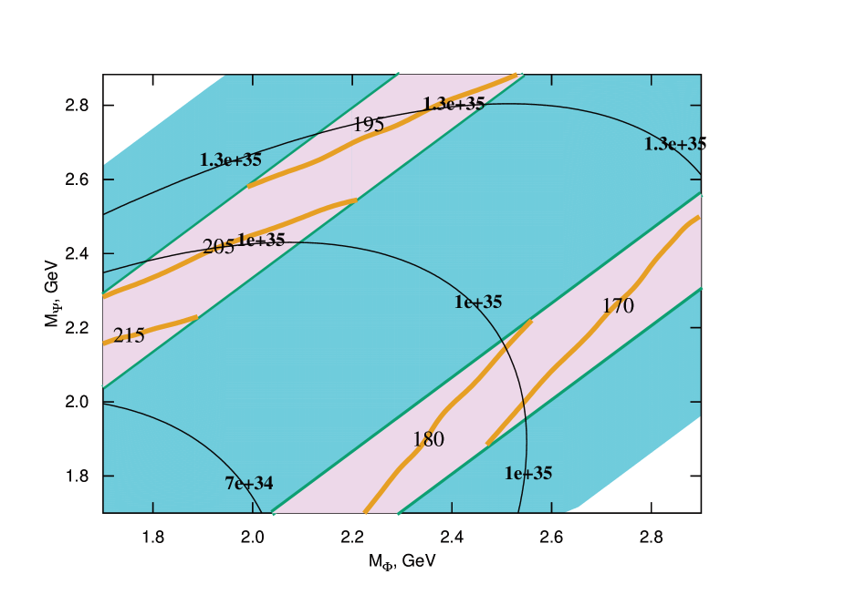
Figure 1: Contours (thin lines) of constant lifetime (in years) of a neutron with respect to the processes $\Psi n\to\Phi\gamma$ and $\Phi n\to\Psi\gamma$, assuming equal number densities of the two dark matter components and parameters $\Lambda=M_{X}=1$ TeV and $y=1$. Present experimental bounds are applicable in the violet (light grey) regions on the plot. Thick lines in these regions show the limits on the quantity $\left(\Lambda^{2}M_{X}/y\right)^{1/3}$ in GeV.

we show contours of the constant neutron lifetime of a neutron (thin lines) with respect to induced neutron-decay processes $\Phi(\Psi)+n\to\Psi(\Phi)+\gamma$. They have been calculated for the realistic set of parameters $\Lambda=M_{X}=1$ TeV and $y=1$ without any cuts on the phase space. As we explained above, the present experimental limit on this process can be applied only within regions shown in violet (light grey) color. In this case, one can obtain the current limit on the characteristic scale of the process $\left(\Lambda^{2}M_{X}/y\right)^{1/3}$; the corresponding bounds are shown in these regions by thick lines. Outside shaded blue (dark grey) and violet (light grey) regions on this and the subsequent similar plots, the stability requirement (4) is not satisfied.

Note in passing, that applying LHC bounds obtained in [11] is not quite straightforward because the couplings $\zeta_{a}$ which enter (11) are not limited directly from these searches. Thus, smaller values of $\Lambda$ and $M_{X}$ may be allowed. However, in this paper we will use $\Lambda=M_{X}=1$ TeV and $y=1$ as a reference set of parameters for numerical estimates.

4 Scattering processes $\Psi(\Phi)+n\to\Phi(\Psi)+e^{+}\,e^{-}$

This is a $2\to 3$ process induced by couplings (13), and (15) through the exchange of a virtual neutron and with emission of virtual photon producing an electron-positron pair. With $p_{+}$ and $p_{-}$ being the 4-momenta of an outcoming positron and electron, the matrix element is

$$\frac{ie^{2}y\beta}{2M_{n}\,\Lambda^{2}}\frac{F_{2}(q^{2})}{M_{X}\,q^{2}}\,\overline{\Psi^{C}}(p_{\Psi})\frac{1+\gamma_{5}}{2}\frac{\hat{p}-M_{n}}{p^{2}-M_{n}^{2}}\sigma^{\mu\nu}q_{\nu}n(p_{n})\Phi\bar{\psi}(p_{+})\gamma^{\mu}\psi(p_{-}).$$

Here $q=p_{+}+p_{-}$, $p=p_{n}-q$ and $\Psi(p_{\Psi})$, $n(p_{n})$, $\psi(p_{+})$, $\psi(p_{-})$ are wave functions of $\Psi$, $n$, $e^{+}$, and $e^{-}$, respectively.

For the squared matrix element of the $2\to 3$ process averaged over spins of two incoming fermions we obtain

$$\begin{split}&\overline{\left|{\cal M}\right|^{2}}=\frac{e^{4}\,y^{2}\,\beta^{2}}{4M_{n}^{2}}\frac{F^{2}_{2}(q^{2})}{M_{X}^{2}\,\Lambda^{4}}\frac{4}{q^{2}}\frac{1}{\left(q^{2}-2qp_{n}\right)^{2}}\,\left(q^{2}\cdot p_{n}p_{+}\cdot qp_{\Psi}+q^{2}\cdot p_{+}p_{\Psi}\cdot qp_{n}\right.\\ &-4qp_{\Psi}\cdot p_{n}p_{+}\cdot p_{n}p_{+}+4p_{n}p_{+}\cdot p_{n}p_{+}\cdot p_{n}p_{\Psi}+2p_{n}p_{+}\cdot qp_{n}\cdot qp_{\Psi}\\ &+q^{2}M_{n}^{2}qp_{\Psi}-q^{2}M_{n}^{2}p_{n}p_{\Psi}-4p_{n}p_{+}\cdot qp_{n}\cdot p_{n}p_{\Psi}-2p_{+}p_{\Psi}\cdot qp_{n}\cdot qp_{n}\\ &+4qp_{n}\cdot p_{+}p_{\Psi}\cdot p_{n}p_{+}-2q^{2}\cdot p_{+}p_{\Psi}\cdot p_{n}p_{+}+2p_{n}p_{\Psi}\cdot qp_{n}\cdot qp_{n}-q^{2}\cdot qp_{n}\cdot p_{n}p_{\Psi}\left.\right).\end{split}$$ (19)

In what follows, it is convenient to describe the final state in terms of energies of the outgoing visible particles by choosing, say, positron energy $E_{+}$ and the sum of positron and electron energies $E$. Then for the scattering $\Psi\,n\to\Phi\,e^{+}e^{-}$, to the leading order in dark matter particle velocity $v\ll 1$, one should make the following substitution in eq. (19) (in both the center-of-mass and the laboratory frames)

$$p_{n}p_{\Psi} =M_{n}M_{\Psi}\,,\;\;\;p_{n}p_{+}=M_{n}E_{+}\,,\;\;\;qp_{n}=EM_{n}\,,$$

$$p_{+}p_{\Psi} =E_{+}M_{\Psi}\,,\;\;\;qp_{\Psi}=EM_{\Psi}\,,\;\;\;qp_{+}=EE_{+}\,,$$

$$q^{2} =2EM-M^{2}+M_{\Phi}^{2}\,,\;\;\;q^{2}-2qp_{n}=2EM_{\Psi}-M^{2}+M_{\Phi}^{2}\,,$$

where we introduced the notation $M=M_{n}+M_{\Psi}$. Finally, we arrive at

$$\begin{split}\overline{\left|{\cal M}\right|^{2}}=&\frac{e^{4}\,y^{2}\,\beta^{2}}{M_{n}^{2}\,q^{2}}\frac{F^{2}_{2}(q^{2})}{M_{X}^{2}\,\Lambda^{4}}\frac{M_{n}\,M_{\Psi}}{\left(q^{2}-2qp_{n}\right)^{2}}\\ &\times\left[q^{2}\left(2E_{+}(E-E_{+})-M_{n}^{2}\right)+2M_{n}^{2}\left(E_{+}^{2}+(E-E_{+})^{2}\right)\right].\end{split}$$

The expression for the differential cross section looks as follows [20]

$$d\sigma=\frac{1}{4I(2\pi)^{3}16s}\,\overline{\left|{\cal M}\right|^{2}}\,dm_{12}^{2}\,dm_{23}^{2}\,,$$

where $I=\sqrt{(p_{n}p_{\Psi})^{2}-M_{n}^{2}M_{\Psi}^{2}}\approx M_{n}M_{\Psi}v$ is a flux factor, and in the nonrelativistic limit, one has $\sqrt{s}=M$. The invariant masses of outgoing pairs (let the subscripts “1” and “2” refer to the visible particles and “3” to the dark matter) in the nonrelativistic limit get reduced to

$$\begin{split}m_{23}^{2}=M^{2}+m_{1}^{2}-2ME_{1}\,,\;\;&m_{12}^{2}=2ME-M^{2}+m_{3}^{2}\\ dm_{12}^{2}\,dm_{23}^{2}=-&2MdE\,2MdE_{1}.\end{split}$$ (20)

The energy $E$ is confined within the interval

$$\frac{(m_{1}+m_{2})^{2}+M^{2}-m_{3}^{2}}{2M}<E<M-m_{3}$$ (21)

and $E_{1}$ is within the interval

$$\frac{m_{1}^{2}+M^{2}-(m_{23}^{2})^{max}}{2M}<E_{1}<\frac{M^{2}+m_{1}^{2}-(m_{23}^{2})_{min}}{2M},$$ (22)

where

$$(m_{23}^{2})^{max}_{min}=2E_{2}^{*}E_{3}^{*}-m_{2}^{2}-m_{3}^{2}\pm 2\sqrt{E_{2}^{*2}-m_{2}^{2}}\sqrt{E_{3}^{*2}-m_{3}^{2}}$$

and

$$E_{3}^{*2}-m_{3}^{2} =\frac{M^{2}((M-E)^{2}-m_{3}^{2})}{2ME-M^{2}+m_{3}^{2}}\,,$$ (23)

$$E_{2}^{*2}-m_{2}^{2} =\frac{(2ME-M^{2}+m_{3}^{2}+m_{2}^{2}-m_{1}^{2})^{2}}{4(2ME-M^{2}+m_{3}^{2})}-m_{2}^{2}\,,$$ (24)

$$2E_{2}^{*}E_{3}^{*} =\frac{(-M^{2}+2ME+m_{3}^{2}+m_{2}^{2}-m_{1}^{2})(M^{2}-ME-m_{3}^{2})}{2ME-M^{2}+m_{3}^{2}}\,.$$ (25)

For the process under discussion, let subscript “1” refer to the positron, and replacing in the above formulas $E_{1}$ with $E_{+}$, we obtain the differential cross section

$$d\sigma=\frac{1}{128\pi^{3}vM_{n}M_{\Psi}}\,\overline{\left|{\cal M}\right|^{2}}\,dE\,dE_{+}$$

which must be integrated over the region defined by eqs. (20)–(25).

For the process $\Phi(p_{\Phi})\,n(p_{n})\to\Psi(p_{\Psi})\,e^{+}(p_{+})e^{-}(p_{-})$, one has the same expression (19) multiplied by a factor of 2 due to one less number of initial fermions and makes the replacement

$$p_{n}p_{+} =M_{n}E_{+}\;,\;\;\;qp_{n}=M_{n}E\;,\;\;\;p_{n}p_{\Psi}=M_{n}(M-E)\,,$$

$$q^{2} =-M^{2}+M_{\Psi}^{2}+2ME\;,\;\;\;p_{+}p_{\Psi}=\frac{1}{2}M^{2}-\frac{1}{2}M_{\Psi}^{2}-M(E-E_{+})\;,$$

$$qp_{\Psi} =M^{2}-M_{\Psi}^{2}-ME\,,\;\;\;q^{2}-2qp_{n}=-M^{2}+M_{\Psi}^{2}+2E(M-M_{n})\;,$$

where $M=M_{\Phi}+M_{n}$.

The current best limit [20, 19] for neutron decay in the mode $n\to\nu e^{+}e^{-}$ is:

$$\tau_{n\to\nu e^{+}e^{-}}>2.57\times 10^{32}\,\text{yr}\;.$$

It has been obtained from the analysis of experimental data with imposing the following cut on the total energy of leptons [5, 19]

$$500\,\text{MeV}\leq E\leq 850\,\text{MeV}$$ (26)

and assuming that the asymmetry is small,

$$A<0.5\,.$$ (27)

The latter quantity characterizes the directional asymmetry of energy release in the Cherenkov detector. The asymmetry is maximal, $A=1$, for collinear particles and equals zero for such a decay, where the particles go in opposite directions. Let us stress, that this quantity counts not all the particles, but only those which release the energy inside the Cherenkov detector, and accounts for them with weights proportional to the energy release into the Cherenkov radiation.

In our case of the electron-positron pair the weights are identical. For the decay $n\to\nu\,e^{+}\,e^{-}$, all 3-momenta of the outgoing particles are in a decay plane. All three particles are relativistic, so the Cherenkov angles for the electron and positron are identical and the energy conservation gives for the sum of the particle energies

$$E_{\nu}+E_{+}+E_{-}=M\,,$$ (28)

where $M$ is the neutron mass. Then the asymmetry defined in [5, 19] is just

$$A\equiv\frac{1}{2}\left(1+{\bf n_{+}}{\bf n_{-}}\right),$$ (29)

where ${\bf n_{\pm}}$ are unit 3-vectors along the direction of the outgoing positron and electron, respectively. Introducing the reference axis along the 3-momentum of the neutrino, one defines corresponding transverse and longitudinal parts of the electron and positron momenta. Obviously, the transverse parts of electron and positron momenta are equal in magnitude but of opposite directions

$$p_{+}^{\perp}=-p_{-}^{\perp},$$ (30)

while the longitudinal parts (momentum projection on the chosen axis) sum to zero,

$$p_{\nu}^{\parallel}+p_{+}^{\parallel}+p_{-}^{\parallel}=0.$$ (31)

For the relativistic electron and positron, one has

$$E_{\pm}^{2}=p_{\pm}^{\parallel\,2}+p_{\pm}^{\perp\,2}$$ (32)

and for relativistic neutrino with the chosen axis $p_{\nu}^{\parallel}>0$ and

$$p_{\nu}^{\parallel}=E_{\nu}.$$ (33)

Then, the asymmetry (29) reads

$$A=\frac{1}{2}\left(1+\frac{p_{+}^{\parallel}}{E_{+}}\frac{p_{-}^{\parallel}}{E_{-}}+\frac{p_{+}^{\perp}}{E_{+}}\frac{p_{-}^{\perp}}{E_{-}}\right).$$ (34)

The differential decay rate is given by

$$d\Gamma=\frac{1}{(2\,\pi)^{3}}\,\frac{1}{32\,M^{3}}\,\overline{\left|{\cal M}\right|^{2}}\,dm_{12}^{2}\,dm_{23}^{2}\,.$$ (35)

Introducing the sum of the electron and positron energies

$$E\equiv E_{+}+E_{-}$$

one obtains for the phase space measure (20) (where $E_{1}$ stands for $E_{+}$) that ranges (21) and (22) are reduced to

$$\frac{M}{2}<E<M\,\;\;\;\;\;E-\frac{M}{2}<E_{+}<\frac{M}{2}\;.$$ (36)

Two independent variables, e.g. $E$ and $E_{+}$, fix all the others, which can be found by solving Eqs. (28), (30), (31), (32) under condition (33). The results read

$$E_{-} =E-E_{+}\,,$$ (37)

$$E_{\nu} =M-E\,,$$ (38)

$$p_{+}^{\parallel} =\frac{E(M-E_{+})-M^{2}/2}{M-E}\,,$$ (39)

$$p_{-}^{\parallel} =\frac{E(M-E)+EE_{+}-M^{2}/2}{E-M}\,,$$ (40)

$$p_{-}^{\perp\,2} =p_{+}^{\perp\,2}=\frac{M(E-M/2)(2E_{+}-M)(E-E_{+}-M/2)}{(E-M)^{2}}.$$ (41)

Putting the solutions above into (34), one obtains for the asymmetry

$$A=\frac{1}{2}\left(1-\frac{E_{+}(E_{+}-E)+M(E-M/2)}{E_{+}(E-E_{+})}\right).$$ (42)

The cut adopted in [5, 19] $A<0.5$ implies a positive value of the second term in parentheses in Eq. (42). It slightly increases the lower limit for $E$ and, thus, reduces a little the triangle integration region in (36).

To adopt the same cuts on asymmetry $A$ in the case of the $2\to 3$ process $\Psi n\to\Phi e^{+}e^{-}$ one can treat it in the nonrelativistic regime as a decay of the particle of effective mass

$$M\approx M_{n}+M_{\Psi}\,.$$

Then the following formulas from the previous considerations must be modified as follows:

• Instead of the massless neutrino, the outcoming dark matter particle $\Phi$ is massive, so its 3-momentum (we use the same notations) instead of (33) obeys

  $$p_{\nu}^{\parallel\,2}+M^{2}_{\Phi}=E_{\nu}^{2},$$ (43)

• The region of integration in Eq. (36)

  $$\frac{M^{2}-M^{2}_{\Phi}}{2M}<E<M-M_{\Phi}\,,\;\;$$ (44)

  $$\frac{1}{2}(E-\sqrt{(M-E)^{2}-M_{\Phi}^{2}})<E_{+}<\frac{1}{2}(E+\sqrt{(M-E)^{2}-M_{\Phi}^{2}}),$$

• Longitudinal momenta are

  $$p_{+}^{\parallel} =\frac{E(M-E_{+})-M^{2}/2+M_{\Phi}^{2}/2}{\sqrt{(M-E)^{2}-M_{\Phi}^{2}}}\,,$$ (45)

  $$p_{-}^{\parallel} =\frac{E(E_{+}+M-E)-M^{2}/2+M_{\Phi}^{2}/2}{\sqrt{(M-E)^{2}-M_{\Phi}^{2}}}\,,$$ (46)

  and the transverse momenta read

  $$p_{-}^{\perp\,2}=p_{+}^{\perp\,2}=\frac{[M(E_{+}-E+M/2)-M_{\Phi}^{2}/2][(E-M/2)(M-2E_{+})+M_{\Phi}^{2}/2]}{(M-E)^{2}-M_{\Phi}^{2}},$$ (47)

• The asymmetry (42) must be replaced with

  $$A=\frac{1}{2}\left(1-\frac{E_{+}(E_{+}-E)+M(E-M/2)+M_{\Phi}^{2}/2}{E_{+}(E-E_{+})}\right).$$ (48)

Similar formulas with evident replacements $M_{\Phi}\to M_{\Psi}$ and $M\to M_{n}+M_{\Phi}$ are applicable for the description of the twin process $\Phi n\to\Psi e^{+}e^{-}$.

For the original process $n\to\nu e^{+}e^{-}$, assuming the momenta-independent matrix element, the cuts (26) and (27) select a 0.3278/0.3904 part of the phase space. In Fig. 2,

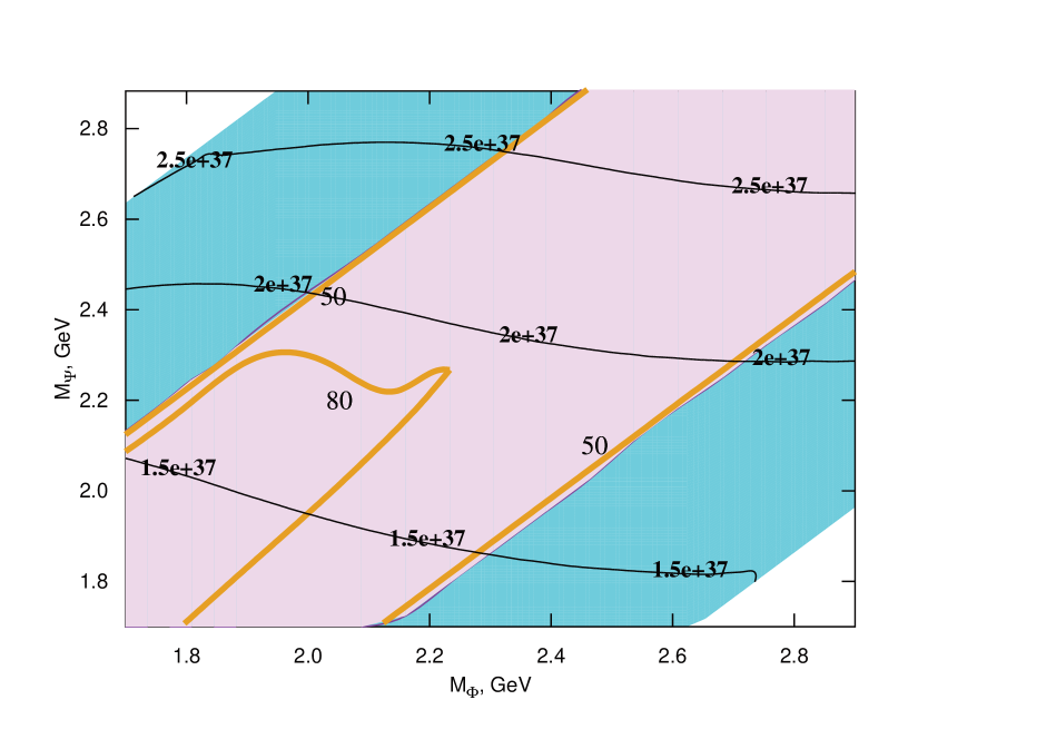
Figure 2: Contours (thin lines) of constant lifetime (in years) of a neutron with respect to the process $\Psi(\Phi)n\to\Phi(\Psi)e^{+}e^{-}$; we set $\Lambda=M_{X}=1$ TeV and $y=1$. Present experimental bounds are applicable in the violet (light grey) region on the plot. Thick lines in this region show the limits on the quantity $\left(\Lambda^{2}M_{X}/y\right)^{1/3}$.

we show contours of the constant lifetime of a neutron (thin lines) with respect to induced neutron decay processes $\Phi(\Psi)+n\to\Psi(\Phi)+e^{+}e^{-}$. They have been calculated without any cuts for $\Lambda=M_{X}=1$ TeV and $y=1$. The current limits on these processes can be applied only within the region shown in violet (light grey) color. They are distinguished by the corresponding kinematics of the process and applied cuts (26), (27). In this case one can obtain the current limit on the characteristic scale of the process $\Lambda$; the corresponding bounds are shown in these regions by thick lines.

Now let us consider the asymmetric case when number densities of $\Psi$ and $\Phi$ are different, $\eta\neq 1$, see eq. (3). As an example, below we consider opposite cases of asymmetry: $\eta=0.01$ and $\eta=100$, which correspond to $\Psi$ or $\Phi$ dominance, respectively. Note that in this case the allowed mass intervals are different from that of the symmetric case. Namely, mass of the dominant component is fixed in the very narrow region around $5M_{p}/2$, while the subdominant component can have mass which is determined by the condition (4). In Fig. 3,

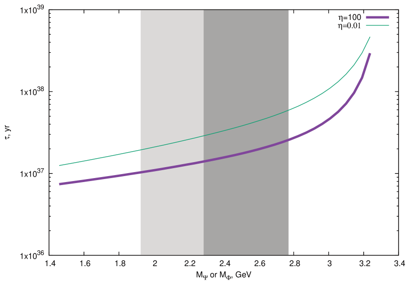
Figure 3: Lifetime of a neutron with respect to IND $n\to e^{+}e^{-}$ for $\eta=100$ and $\eta=0.01$; we set $\Lambda=M_{X}=1$ TeV and $y=1$. The current limits are applied in shaded regions.

we show expected lifetimes of a neutron with respect to the processes $\Phi(\Psi)+n\to\Psi(\Phi)+e^{+}e^{-}$ for the cases of $\Phi$ and $\Psi$ dominance calculated for the same set of parameters as we described previously. The current limits on this process are applicable in the shaded regions on these figures and they (almost uniformly over these regions) result in $\Lambda>35$ GeV ($\eta=100$) and $\Lambda>40$ GeV ($\eta=0.01$) for region 1 and $\Lambda>86$ GeV ($\eta=100$) and $\Lambda>75$ GeV ($\eta=0.01$) for region 2.

Similar plots for the processes $\Phi(\Psi)+n\to\Psi(\Phi)+\gamma$ are shown in Fig. 4. Here one can obtain the following limits on $\Lambda$: for $\eta=100$, we have $\Lambda>215-228$ GeV, and for $\eta=0.01$, we obtain $\Lambda>185-200$ GeV depending on the mass of the subdominant component.

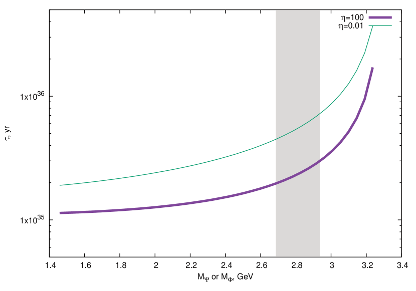
Figure 4: Lifetime of a neutron with respect to the processes $\Phi+n\to\Psi+\gamma$ (for $\eta=100$) and $\Psi+n\to\Phi+\gamma$ (for $\eta=0.01$); we set $\Lambda=M_{X}=1$ TeV and $y=1$.

5 Processes $\Psi(\Phi)+N\to\Phi(\Psi)+2$ mesons

Within the chiral perturbation theory, the IND processes with two mesons in the final state arise in the $1/f^{2}$ order due to the following terms in the low-energy effective lagrangian

$${\cal L}_{1\pi}=i\,\frac{c_{1}\beta}{f}\,\Phi\overline{\Psi^{C}}\left(-\sqrt{\frac{3}{2}}n\eta+\frac{1}{\sqrt{2}}n\pi^{0}-p\pi^{-}\right)+\text{h.c.}\,,$$ (49)

$$\begin{split}{\cal L}_{2\pi}=-\frac{\beta\,c_{1}}{2f^{2}}\left(\sqrt{6}\pi^{-}\eta+K^{0}{K}^{-}\right)\Phi\,\overline{\Psi^{C}}p_{R}\\ -\frac{\beta\,c_{1}}{2f^{2}}\left(\pi^{+}\pi^{-}+\frac{3}{2}\eta^{2}-\sqrt{3}\eta\pi^{0}+\frac{1}{2}(\pi^{0})^{2}+2K^{0}\bar{K}^{0}+K^{+}K^{-}\right)\Phi\,\overline{\Psi^{C}}n_{R}+\text{h.c.}\,,\end{split}$$ (50)

with parameter $c_{1}$ related to the model parameters as follows from matching eqs. (11) and (12) to eqs. (68) and (69)

$$c_{1}=\frac{y}{M_{X}\Lambda^{2}}\,.$$

Details of the derivation are presented in the Appendix A for completeness. Below, we work in the limit of exact isotopic invariance, neglecting the proton-neutron and charged-neutral pion mass differences,

$$M_{n}=M_{p}\equiv M_{N}\,,\;\;\;\;m_{\pi^{+}}=m_{\pi^{0}}\equiv m_{\pi}\,,\;\;\;\;m_{K^{+}}=m_{K^{0}}\equiv m_{K}\;.$$

Two types of diagrams contribute the processes: one of them follows from lagrangian (50) and the other comes from one-meson lagrangian (49), while the second meson is radiated from the nucleon leg; see eq. (72).

For the $dud$ operator, we have the following possibilities for induced decays, which we classify here according to the number of tree-level Feynman diagrams contributing the corresponding process:

• one-diagram processes $p\to\bar{K}^{0}K^{+}$, $n\to K^{0}\bar{K}^{0}$, and $n\to K^{+}K^{-}$;

• two-diagram processes $p\to\pi^{0}\pi^{+}$, $n\to\pi^{+}\pi^{-}$;

• three-diagram processes $n\to\eta\pi^{0}$, $p\to\eta\pi^{+}$, $n\to\eta\eta$, and $n\to\pi^{0}\pi^{0}$.

One-diagram processes.

The Feynman diagram for the process $\Psi+p\to\Phi+\bar{K}^{0}K^{+}$ is presented in Fig. 5

Figure 5: The Feynman diagrams for the process $\Psi+p\to\Phi+\bar{K}^{0}K^{+}$ .

Averaged over spins of the two initial fermions, the squared matrix element of this process reads

$$\overline{\left|{\cal M}\right|^{2}}=\frac{\beta^{2}c^{2}_{1}}{8f^{4}}\,p_{N}p_{\Psi}\,,$$ (51)

and by a factor of two bigger for $\Phi+p\to\Psi+\bar{K}^{0}K^{+}$; hereafter, $p_{N}$ refers to the 4-momentum of the nucleon participating in the corresponding process. For the first process, in the laboratory frame one has to the leading order in dark matter velocity

$$p_{N}p_{\Psi}=M_{N}\,M_{\Psi}$$ (52)

and when integrating over the phase space adopts the formulas (20)–(25) with

$$M=M_{N}+M_{\Psi}\;,\;\;m_{1}=m_{2}=m_{K}\,,\;\;\;m_{3}=M_{\Phi}\,.$$ (53)

Instead, for the second process we have

$$M=M_{N}+M_{\Phi}\,,\;\;p_{N}p_{\Psi}=M_{N}\,\left(M-E\right)\,,\;\;m_{1}=m_{2}=m_{K}\,,\;\;m_{3}=M_{\Psi}.$$ (54)

Averaged over spins of the initial two fermions, squared matrix element of the process $\Psi+n\to\Phi+K^{-}K^{+}$ reads as (51) and by a factor of two bigger for $\Phi+n\to\Psi+K^{-}K^{+}$. Further, in the laboratory frame one can use eqs. (52), (53) and eq. (54) for the first and second processes, respectively. The same sets of formulas work for the processes $\Psi+n\to\Phi+\bar{K}^{0}K^{0}$ and $\Phi+n\to\Psi+\bar{K}^{0}K^{0}$, respectively.

Two-diagram processes.

To describe this class of processes it is convenient to introduce the following notations

$$I(p_{1},p_{2}) \equiv 2\,p_{1}p_{2}-p_{2}^{2}\,,$$ (55)

$$J(p_{1},p_{2},p_{3}) \equiv 2\,p_{1}p_{3}\cdot p_{2}p_{3}-p_{3}^{2}\cdot p_{1}p_{2}\,,$$ (56)

$$K(p_{1},p_{2},p_{3},p_{4}) \equiv p_{1}p_{3}\cdot p_{2}p_{4}+p_{1}p_{4}\cdot p_{2}p_{3}-p_{1}p_{2}\cdot p_{3}p_{4}\,.$$ (57)

The Feynman diagrams for the process $\Psi+p\to\Phi+\pi^{+}\pi^{0}$ are presented in Fig. 6.

Figure 6: The Feynman diagrams for the process $\Psi+p\to\Phi+\pi^{+}\pi^{0}$.

The squared matrix element of this process, averaged over spins of initial particles is

$$\begin{split}\overline{\left|{\cal M}\right|^{2}}=&\frac{(D+F)^{2}c_{1}^{2}\beta^{2}M_{N}^{2}}{f^{4}}\\ &\times\left(\frac{J(p_{N},p_{\Psi},p_{\pi^{+}})}{I^{2}(p_{N},p_{\pi^{+}})}+\frac{J(p_{N},p_{\Psi},p_{\pi^{0}})}{I^{2}(p_{N},p_{\pi^{0}})}-\frac{2K(p_{N},p_{\Psi},p_{\pi^{+}},p_{\pi^{0}})}{I(p_{N},p_{\pi^{+}})\,I(p_{N},p_{\pi^{0}})}\right),\end{split}$$ (58)

where $D=0.8$ and $F=0.47$ (see the Appendix A). In the laboratory frame, one has

$$p_{N}p_{\Psi} =M_{N}M_{\Psi}\,,\;\;\;p_{N}p_{\pi^{0}}=M_{N}(E-E_{1}),\;\;\;p_{N}p_{\pi^{+}}=M_{N}E_{1}\,,$$

$$p_{\pi^{0}}p_{\Psi} =\left(E-E_{1}\right)M_{\Psi}\,,\;\;\;p_{\pi^{+}}p_{\Psi}=E_{1}M_{\Psi}\,,\;\;\;p_{\pi^{+}}p_{\pi^{0}}=EM-m_{\pi}^{2}+\frac{1}{2}\left(M_{\Phi}^{2}-M^{2}\right)\,,$$

and adopts eqs.(20)–(25) with

$$M=M_{\Psi}+M_{N},\;\;m_{1}=m_{2}=m_{\pi}\,,\;\;\;m_{3}=M_{\Phi}\,.$$

For $\Phi+p\to\Psi+\pi^{+}\pi^{0}$, one obtains for the squared averaged matrix element (58) but a factor of two bigger. In the laboratory frame, one finds

$$p_{N}p_{\Psi} =M_{N}\left(M-E\right)\,,\;\;p_{\pi^{0}}p_{\Psi}=\frac{1}{2}\left(M^{2}-M_{\Psi}^{2}\right)-E_{1}M\,,$$

$$p_{N}p_{\pi^{0}} =M_{N}(E-E_{1})\,,\;\;p_{\pi^{+}}p_{\pi^{0}}=EM-m_{\pi}^{2}+\frac{1}{2}\left(M_{\Psi}^{2}-M^{2}\right)\,,$$

$$p_{N}p_{\pi^{+}} =M_{N}E_{1}\,,\;\;p_{\pi^{+}}p_{\Psi}=\frac{1}{2}\left(M^{2}-M_{\Psi}^{2}\right)-\left(E-E_{1}\right)M\,,$$

with

$$M=M_{\Phi}+M_{N}\,,\;\;\;m_{1}=m_{2}=m_{\pi}\,,\;\;\;m_{3}=M_{\Psi}\,.$$

The predictions of the proton decay with $\pi^{+}\pi^{0}$ final state are presented in Fig. 7 as contours of the constant lifetime for the symmetric case $\eta=1$. Again, here and below we fix $\Lambda=M_{X}=1$ TeV and $y=1$ and impose no cuts in the phase space.

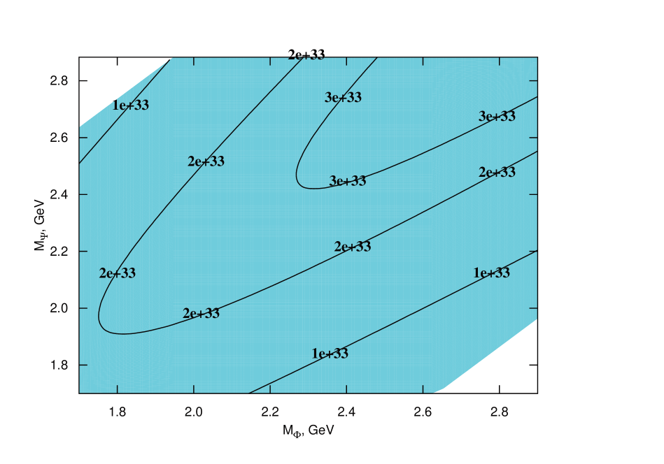
Figure 7: Contours of constant lifetime (in years) of the nucleon in the symmetric case with respect to IND process with $\pi^{+}\pi^{0}$ in the final state; we set $\Lambda=M_{X}=1$ TeV and $y=1$.

Another two-diagram IND process is $\Psi+n\to\Phi+\pi^{+}\pi^{-}$. Corresponding Feynman diagrams are presented in Fig. 8.

Figure 8: The Feynman diagrams for the process $\Psi+n\to\Phi+\pi^{+}\pi^{-}$ .

The squared matrix element of $\Psi+n\to\Phi+\pi^{+}\pi^{-}$ averaged over spins of the initial particles takes the form

$$\frac{1}{2}(A-B)^{2}\,p_{N}p_{\Psi}+2B(A-B)\,\frac{M_{N}^{2}\,p_{\Psi}p_{\pi^{-}}}{I(p_{N},p_{\pi^{-}})}+2B^{2}M_{N}^{2}\frac{J(p_{N},p_{\Psi},p_{\pi^{-}})}{I^{2}(p_{N},p_{\pi^{-}})}.$$

where

$$A=\frac{\beta c_{1}}{2f^{2}}\,,\;\;\;B=\frac{(F+D)\beta c_{1}}{f^{2}}.$$

In the laboratory frame, one has the same expression as (64), (65) for pions. For $\Phi+n\to\Psi+\pi^{+}\pi^{-}$, one has a factor of two bigger squared averaged matrix element and the same expressions in the laboratory frame as (66) and (67) for pions.

Three-diagram processes.

The Feynman diagrams for the process $\Psi+p\to\Phi+\pi^{+}\eta$ are presented in Fig. 9.

Figure 9: The Feynman diagrams for the process $\Psi+p\to\Phi+\pi^{+}\eta$ .

The squared matrix elements of the processes $\Psi+p\to\Phi+\pi^{+}\eta$ and $\Psi+n\to\Phi+\pi^{0}\eta$, averaged over spins of the initial particles have the form

$$\overline{\left|{\cal M}\right|^{2}}=2M_{N}^{2}\left(B^{2}\frac{J(p_{N},p_{\Psi},p_{\pi^{+}})}{I^{2}(p_{N},p_{\pi^{+}})}+C^{2}\frac{J(p_{N},p_{\Psi},p_{\eta})}{I^{2}(p_{N},p_{\eta})}+2BC\frac{K(p_{N},p_{\Psi},p_{\pi^{+}},p_{\eta})}{I(p_{N},p_{\pi^{+}})\,I(p_{N},p_{\eta})}\right)$$

$$+\frac{1}{2}(A-B-C)^{2}\,p_{N}p_{\Psi}+2B(A-B-C)\frac{M_{N}^{2}\,p_{\pi^{+}}p_{\Psi}}{I(p_{N},p_{\pi^{+}})}+2C(A-B-C)\frac{M_{N}^{2}\,p_{\eta}p_{\Psi}}{I(p_{N},p_{\eta})},$$

where

$$A=\frac{\sqrt{6}\beta c_{1}}{2f^{2}},\;\;\;B=\sqrt{\frac{3}{2}}\frac{(D+F)\beta c_{1}}{f^{2}},\;\;\;C=\frac{(3F-D)\beta c_{1}}{\sqrt{6}f^{2}}$$ (59)

for $\Psi+p\to\Phi+\pi^{+}\eta$ and

$$A=\frac{\sqrt{3}\beta c_{1}}{2f^{2}},\;\;\;B=\frac{\sqrt{3}(D+F)\beta c_{1}}{2f^{2}},\;\;\;C=\frac{(3F-D)\beta c_{1}}{2\sqrt{3}f^{2}}$$ (60)

for $\Psi+n\to\Phi+\pi^{0}\eta$. In the laboratory frame, one has

$$p_{N}p_{\Psi} =M_{N}M_{\Psi}\,,\;\;\;p_{\Psi}p_{\eta}=M_{\Psi}(E-E_{1})\,,\;\;\;\,p_{N}p_{\pi^{+}}=M_{N}E_{1}\,,$$

$$p_{N}p_{\eta} =\left(E-E_{1}\right)M_{N}\,,\;\;2\,p_{\pi^{+}}p_{\eta}=M\left(2E-M\right)+M_{\Phi}^{2}-m_{\pi}^{2}-m_{\eta}^{2}\,,\;\;p_{\pi^{+}}p_{\Psi}=E_{1}M_{\Psi}\,,$$

and utilizes eqs. (20)–(25) with

$$M=M_{\Psi}+M_{N}\,\;\;\;m_{1}=m_{\pi}\,,\;\;\;m_{2}=m_{\eta}\,,\;\;\;m_{3}=M_{\Phi}\,.$$

For processes $\Phi+p\to\Psi+\pi^{+}\eta$ and $\Phi+n\to\Psi+\pi^{0}\eta$, one multiplies the above expression for the squared averaged matrix element by a factor of 2 and makes the following substitutions

$$2\,p_{\pi^{+}}p_{\Psi} =M\left(M+2E_{1}-2E\right)-M_{\Psi}^{2}-m_{\pi}^{2}+m_{\eta}^{2}\,,$$

$$p_{N}p_{\Psi} =M_{N}(M-E)\,,\;\;\;2\,p_{\Psi}p_{\eta}=M\left(M-2E_{1}\right)-M_{\Psi}^{2}+m_{\pi}^{2}-m_{\eta}^{2}\,,$$

$$p_{N}p_{\pi^{+}} =M_{N}E_{1}\,,\;\;p_{N}p_{\eta}=\left(E-E_{1}\right)M_{N}\,,\;\;2\,p_{\pi^{+}}p_{\eta}=M\left(2E-M\right)+M_{\Psi}^{2}-m_{\pi}^{2}-m_{\eta}^{2}\,,$$

and uses eqs. (20)–(25) with

$$M=M_{\Phi}+M_{N}\,,\;\;\;m_{1}=m_{\pi}\,,\;\;\;m_{2}=m_{\eta}\,,\;\;\;m_{3}=M_{\Psi}\,.$$

Predictions for the proton lifetime for the $\pi^{+}\eta$ final state and neutron lifetime for $\pi^{0}\eta$ final state are presented for the symmetric case in Fig, 10 and Fig. 11, respectively.

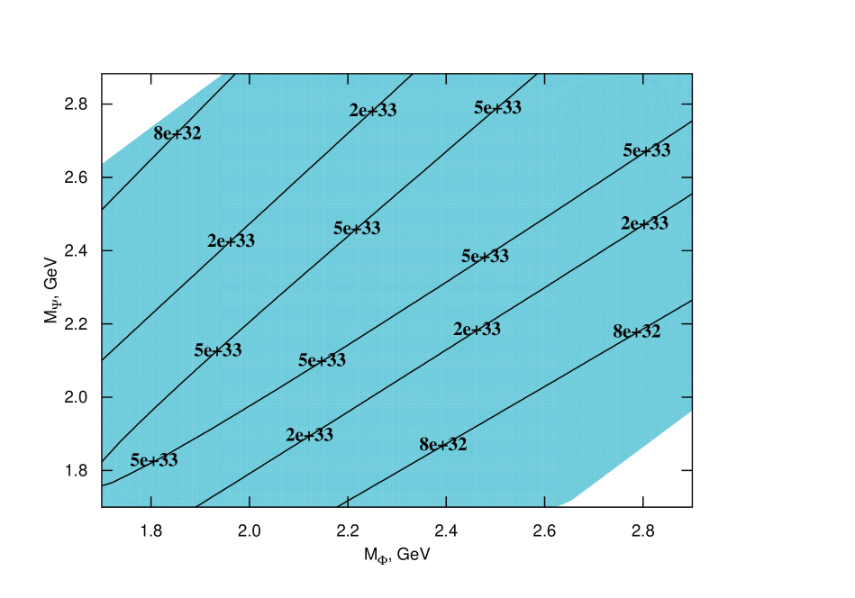
Figure 10: Contours of the constant lifetime (in years) of a nucleon in the symmetric case with respect to IND with $\pi^{+}\eta$ in the final state; we set $\Lambda=M_{X}=1$ TeV and $y=1$.

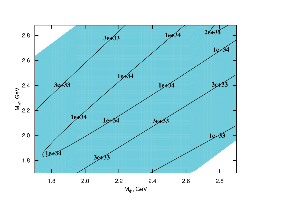
Figure 11: Contours of the constant lifetime (in years) of a nucleon in the symmetric case with respect to IND with $\pi^{0}\eta$ in the final state; we set $\Lambda=M_{X}=1$ TeV and $y=1$.

The squared matrix element for the processes $\Psi+n\to\Phi+2\eta$ and $\Psi+n\to\Phi+2\pi^{0}$ averaged over spins of the initial particles have the form

$$\begin{split}\overline{\left|{\cal M}\right|^{2}}=&2(A-B)^{2}\,p_{N}p_{\Psi}+4B(A-B)\frac{M_{N}^{2}\,p_{1}p_{\Psi}}{I(p_{N},p_{1})}+4B(A-B)\frac{M_{N}^{2}\,p_{2}p_{\Psi}}{I(p_{N},p_{2})}\\ &+2B^{2}M_{N}^{2}\left(\frac{J(p_{N},p_{\Psi},p_{1})}{I^{2}(p_{N},p_{1})}+\frac{J(p_{N},p_{\Psi},p_{2})}{I^{2}(p_{N},p_{2})}+2\frac{K(p_{N},p_{\Psi},p_{1},p_{2})}{I(p_{N},p_{1})I(p_{N},p_{2})}\right),\end{split}$$ (61)

where $p_{1}$ and $p_{2}$ are momenta of outgoing mesons and

$$A=\frac{3\beta c_{1}}{4f^{2}},\;\;\;B=\frac{(3F-D)\beta c_{1}}{2f^{2}}$$ (62)

for $\Psi+n\to\Phi+2\eta$ and

$$A=\frac{\beta c_{1}}{4f^{2}},\;\;\;B=\frac{(D+F)\beta c_{1}}{2f^{2}}$$ (63)

for $\Psi+n\to\Phi+2\pi^{0}$. In the laboratory frame one has

$$\begin{split}&p_{N}p_{1}=M_{N}E_{1}\,,\;\;p_{\Psi}p_{2}=M_{\Psi}(E-E_{1})\,,\;\;2\,p_{1}p_{2}=M\left(2E-M\right)+M_{\Phi}^{2}-2m_{1}^{2}\,,\\ &p_{N}p_{2}=\left(E-E_{1}\right)M_{N}\,,\;\;\;p_{N}p_{\Psi}=M_{N}M_{\Psi}\,,\;\;\;p_{1}p_{\Psi}=E_{1}M_{\Psi}\,,\end{split}$$ (64)

and adopts eqs. (20)–(25) with

$$M=M_{\Psi}+M_{N}\,,m_{3}=M_{\Phi}\,,\;\;\;\text{and}\;\;m_{1}=m_{2}=m_{\pi,\eta}\,.$$ (65)

For the averaged squared matrix elements of $\Phi+n\to\Psi+2\eta$ and $\Phi+n\to\Psi+2\pi^{0}$, one has the same expression (61) multiplied by a factor of two. In the laboratory frame, one finds

$$\begin{split}&2\,p_{1}p_{\Psi}=M\left(M+2E_{1}-2E\right)-M_{\Psi}^{2}\,,\;\;\;p_{N}p_{1}=M_{N}E_{1}\,,\\ &2\,p_{\Psi}p_{2}=M\left(M-2E_{1}\right)-M_{\Psi}^{2}\,,\;\;\;\,p_{N}p_{\Psi}=M_{\Psi}(M-E)\,,\\ &p_{N}p_{2}=\left(E-E_{1}\right)M_{N}\,,\;\;\;2\,p_{1}p_{2}=M\left(2E-M\right)+M_{\Psi}^{2}-2m_{\pi,\eta}^{2}\,,\end{split}$$ (66)

and adopts eqs. (20)–(25) with

$$M=M_{\Phi}+M_{N}\,,m_{3}=M_{\Psi}\,,\;\;\;\text{and}\;\;m_{1}=m_{2}=m_{\pi,\eta}\,.$$ (67)

In Fig. 12

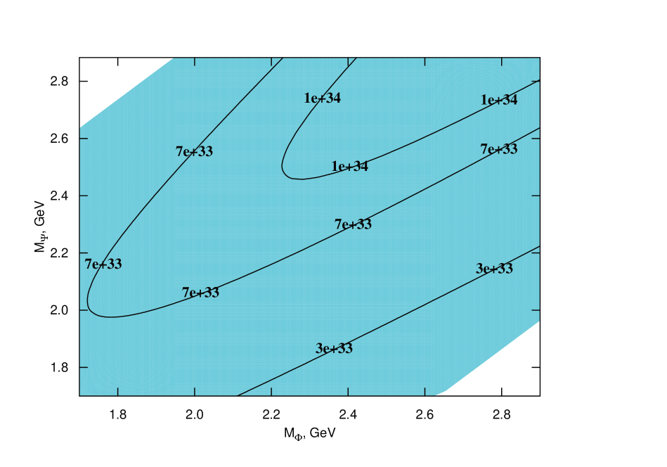
Figure 12: Contours of the constant lifetime (in years) of a nucleon in the symmetric case with respect to IND process with $\pi^{0}\pi^{0}$ in the final state; we set $\Lambda=M_{X}=1$ TeV and $y=1$.

we present the predictions of neutron lifetime for the final state $\pi^{0}\pi^{0}$.

Finally, to illustrate a dependence of the obtained predictions on the value of nonspecified asymmetry between $\Psi$ and $\Phi$ populations, $\eta$, we present in Figs. 13 and 14

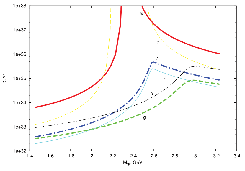
Figure 13: Contours of the constant lifetime (in years) of the nucleon in the asymmetric case, $\eta=100$ , with respect to the two-meson processes: a) $\bar{K}^{0}K^{+}$; b) $\eta\eta$; c) $\pi^{0}\eta$; d) $\pi^{+}\eta$; e) $\pi^{0}\pi^{0}$; g) $\pi^{+}\pi^{0}$. Numbers for other processes with kaons are similar to a) while for process with $\pi^{+}\pi^{-}$ are similar to g). We set $\Lambda=M_{X}=1$ TeV and $y=1$.

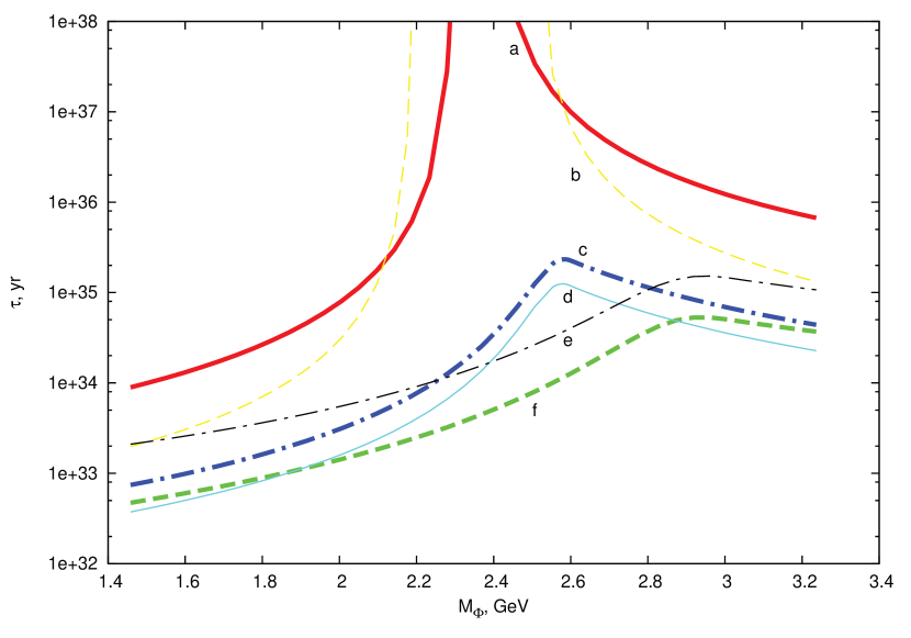
Figure 14: Contours of the constant lifetime (in years) of a nucleon in the asymmetric case, $\eta=0.01$ , with respect to the two-meson processes. Other notations are the same as in Fig. 13.

the estimates of the nucleon lifetime for two opposite cases of large asymmetry $\eta=100$ and $\eta=0.01$, respectively. As one observes, the predictions of nucleon lifetimes within hylogenesis model can reach values around $10^{32}-10^{33}$ year which looks quite promising for future experiments such as Hyper-Kamiokande [1, 16] or DUNE [17].

The obtained predictions for double meson channels are, in general, only by an order of magnitude weaker than those for single-meson channels (which can be as low as several units of $10^{31}$ yr [9, 10] for the same set of parameters). Note that the double meson signatures are predicted for the proton decay in the context of grand unified theories [8] as well as for dinucleon decays such as $pn\to\pi^{+}\pi^{0}$, for instance, in supersymmetric models with R-parity violation; see e.g., [7]. Searches for the latter type of processes had been performed by the Frejus experiment [4] and recently by the Super-Kamiokande collaboration [14]. The most stringent limit for the lifetime of the process $pn\to\pi^{+}\pi^{0}$ per oxygen nucleus is found to be $\tau_{pn\to\pi^{+}\pi^{0}}>1.70\times 10^{32}$ year. It has been obtained by making use of the expected kinematics of dinucleon decay. In particular, the angular distribution between outgoing pions exhibits a maximum for events with back-to-back topology and the distribution over momentum of $\pi^{0}$ has a pronounced peak around nucleon mass. Because of this specific kinematics, the Super-Kamiokande result cannot be directly applied to the IND process with two pions in the final state. However, one can show that for some combinations of masses of dark matter particles, the distributions over momenta of outgoing mesons also have maxima at $0.5-1$ GeV. This signature can be very helpful in discriminating the IND process from the main background which is the double pion production by atmospheric neutrinos.

The double meson channels provide additional signatures of the hylogenesis model, which will help to pin down the relevant model parameters once the signal is found. Indeed, even the masses of dark matter particles cannot be unambiguously extracted from a single-meson event, because the initial nucleon momentum is not fixed in a real experiment (the nucleon is not at rest); hence, the single mesons are not monochromatic. A joint analysis of single and double meson events can help to resolve the parameter values. Generally, one anticipates that having more than one observable particle in the final state gives more opportunities for background reduction in the future experiments.

The two-meson channels even can help to discriminate between proton decay and induced proton decay, which may be challenging is some situations. In particular, if single pions are registered at sub-GeV range (say, below 500 MeV), an observation of multi-pion events with higher total energies would favor the proton decay over the induced proton decay in a model where the kinematics constrains the amount of energy allocated to pion at sub-GeV range.

6 Conclusions

Summarizing, in this paper we calculated the cross sections of several IND processes for the hylogenesis model of dark matter. They include the processes of mimicking neutron decays $n\to\nu\gamma$ and $n\to e^{+}e^{-}$. Applying current best limits on the neutron lifetime with respect to the processes $n\to\nu\gamma$ and $n\to e^{+}e^{-}$ and taking into account the kinematics of the processes which were used in the experiment, we obtained constraints on the parameter space of the model. They are considerably weaker than the bounds obtained using the results of the searches for events with a high $p_{T}$ jet and missing energy signature at LHC experiments.

Also, we calculated cross sections and lifetimes corresponding to IND processes with two pions in the final state. Searches for such kinds of signatures have not been performed yet and present an interesting possibility to further explore the hylogenesis model. We found that with the current bounds from the LHC data, the model allows for a lifetime of IND such as $p\to\pi^{+}\pi^{0}$ or $n\to\pi^{0}\eta$ at the level of $2\times 10^{32}$ yr.

Note in passing, that by the time the new generation of experiments looking for nucleon decay will be in operation, more data from Run2 of the LHC allow an improvement of the collider sensitivity to hylogenesis with respect to the analysis [11].

The work was supported by the RSCF grant 14-12-01430.

Appendix A Couplings to baryons and mesons

The interaction lagrangian of the type (11) with the three light quarks $q_{1}=u$, $q_{2}=d$, $q_{3}=s$ in terms of two-component spinors (the relevant are right-handed parts of the Dirac spinors) has the form [10]

$${\cal L}_{int}=\text{Tr}\left({\cal C}\,{\cal O}\right)+\text{h.c.}\,,\;\;\;\;{\cal O}_{ij}\equiv\frac{1}{2}\,\Phi\,\epsilon_{\alpha\beta\gamma}\epsilon_{jkl}\,\,{q_{k}}_{R}^{\alpha}{q_{l}}_{R}^{\beta}\,\,{q_{i}}_{R}^{\gamma}\Psi_{R}\,,$$ (68)

where

$${\cal C}\equiv\left(\begin{array}[]{ccc}\frac{c_{2}}{\sqrt{6}}+\frac{c_{3}}{\sqrt{2}}&0&0\\ 0&\frac{c_{2}}{\sqrt{6}}-\frac{c_{3}}{\sqrt{2}}&0\\ 0&c_{1}&-\sqrt{\frac{2}{3}}\,c_{2}\\ \end{array}\right).$$ (69)

The couplings $c_{i}$ are introduced as couplings to the three-quark states which form the eigenstates of the strong isospin operator.

Using the chiral perturbation theory one can obtain [8] the corresponding interaction lagrangian for baryons

$${\cal L}_{IND}=\beta\,\text{Tr}\left(\Phi\xi{\cal C}\xi^{\dagger}\,{\cal B}_{R}\Psi_{R}\right)+\text{h.c.},$$

where $\xi={\rm exp}\left(i{\cal M}/f\right)$ and

$${\cal M}\equiv\left(\begin{array}[]{ccc}\frac{\eta}{\sqrt{6}}+\frac{\pi^{0}}{\sqrt{2}}&\pi^{+}&K^{+}\\ \pi^{-}&\frac{\eta}{\sqrt{6}}-\frac{\pi^{0}}{\sqrt{2}}&K^{0}\\ K^{-}&\bar{K}^{0}&-\sqrt{\frac{2}{3}}\eta\\ \end{array}\right)$$

and baryon fields leaving only a neutron and proton

$${\cal B}_{R}=\left(\begin{array}[]{ccc}0&0&p_{R}\\ 0&0&n_{R}\\ 0&0&0\\ \end{array}\right).$$

Expanding to linear order in meson fields we find (hereafter, in terms of the Dirac fermions)

$$\begin{split}{\cal L}_{1\pi}=\frac{i\beta}{f}\,\Phi\,\overline{\Psi^{C}}\,\Bigg{[}&c_{1}\left(-\sqrt{\frac{3}{2}}n_{R}\,\eta+\frac{1}{\sqrt{2}}n_{R}\,\pi^{0}-p_{R}\,\pi^{-}\right)\\ &+\left(\frac{c_{2}\sqrt{3}}{\sqrt{2}}+\frac{c_{3}}{\sqrt{2}}\right)p_{R}\,K^{-}+\left(\frac{c_{2}\sqrt{3}}{\sqrt{2}}-\frac{c_{3}}{\sqrt{2}}\right)n_{R}\,\bar{K}^{0}\Bigg{]}+\text{h.c.}\end{split}$$ (70)

Expanding to the second order in $1/f$, one obtains

$${\cal L}_{2\pi}=\frac{\beta}{2f^{2}}\left(A_{31}\cdot\overline{\Psi^{C}}p_{R}\,\Phi+A_{32}\cdot\overline{\Psi^{C}}n_{R}\,\Phi\right)+\text{h.c.}$$ (71)

where

$$A_{31}= -c_{1}\left(\sqrt{6}\pi^{-}\eta+K^{0}{K}^{-}\right)$$

$$+\left(\frac{3}{2}c_{2}+\frac{\sqrt{3}}{2}c_{3}\right)K^{-}\eta+\left(\frac{\sqrt{3}}{2}c_{2}+\frac{1}{2}c_{3}\right)K^{-}\pi^{0}+\left(\sqrt{\frac{3}{2}}c_{2}-\frac{3}{\sqrt{2}}c_{3}\right)\bar{K}^{0}\pi^{-},$$

$$A_{32}= -c_{1}\left(\pi^{+}\pi^{-}+\frac{3}{2}\eta^{2}-\sqrt{3}\eta\pi^{0}+\frac{1}{2}(\pi^{0})^{2}+2K^{0}\bar{K}^{0}+K^{+}K^{-}\right)$$

$$+\left(\frac{\sqrt{3}}{\sqrt{2}}c_{2}+\frac{3c_{3}}{\sqrt{2}}\right)K^{-}\pi^{+}+\left(\frac{3}{2}c_{2}-\frac{\sqrt{3}}{2}c_{3}\right)\bar{K}^{0}\eta-\left(\frac{\sqrt{3}}{2}c_{2}-\frac{c_{3}}{2}\right)\bar{K}^{0}\pi^{0}.$$

Finally, for completeness let us remind [8] here the interaction lagrangian of baryons with mesons to the leading order in derivative expansion, which has the form

$$\begin{split}{\cal L}=\frac{3F-D}{\sqrt{6}\,f}\left(\bar{p}\gamma^{\mu}\gamma^{5}p+\bar{n}\gamma^{\mu}\gamma^{5}n\right)\partial_{\mu}\eta+\frac{D+F}{\sqrt{2}}\left(\bar{p}\gamma^{\mu}\gamma^{5}p-\bar{n}\gamma^{\mu}\gamma^{5}n\right)\partial_{\mu}\pi^{0}\\ +\frac{D+F}{f}\left(\partial_{\mu}\pi^{+}\bar{p}\gamma^{\mu}\gamma^{5}n+\partial_{\mu}\pi^{-}\bar{n}\gamma^{\mu}\gamma^{5}p\right)\;,\end{split}$$ (72)

where $D=0.8$ and $F=0.47$.

References

- [1] K. Abe et al. Letter of Intent: The Hyper-Kamiokande Experiment — Detector Design and Physics Potential —. 2011.
- [2] Howard Baer, Ki-Young Choi, Jihn E. Kim, and Leszek Roszkowski. Dark matter production in the early Universe: beyond the thermal WIMP paradigm. Phys.Rept., 555:1–60, 2014.
- [3] Nicole F. Bell, Shunsaku Horiuchi, and Ian M. Shoemaker. Annihilating Asymmetric Dark Matter. Phys.Rev., D91(2):023505, 2015.
- [4] Christoph Berger et al. Lifetime limits on (B-L) violating nucleon decay and dinucleon decay modes from the Frejus experiment. Phys. Lett., B269:227–233, 1991.
- [5] G. Blewitt, H.S. Park, B.G. Cortez, G.W. Foster, W. Gajewski, et al. Experimental Limits on the Nucleon Lifetime for Two and Three-body Decay Modes. Phys.Rev.Lett., 54:22, 1985.
- [6] Nikita Blinov, David E. Morrissey, Kris Sigurdson, and Sean Tulin. Dark Matter Antibaryons from a Supersymmetric Hidden Sector. Phys.Rev., D86:095021, 2012.
- [7] Marc Chemtob. Phenomenological constraints on broken R parity symmetry in supersymmetry models. Prog. Part. Nucl. Phys., 54:71–191, 2005.
- [8] Mark Claudson, Mark B. Wise, and Lawrence J. Hall. Chiral Lagrangian for Deep Mine Physics. Nucl.Phys., B195:297, 1982.
- [9] Hooman Davoudiasl, David E. Morrissey, Kris Sigurdson, and Sean Tulin. Hylogenesis: A Unified Origin for Baryonic Visible Matter and Antibaryonic Dark Matter. Phys.Rev.Lett., 105:211304, 2010.
- [10] Hooman Davoudiasl, David E. Morrissey, Kris Sigurdson, and Sean Tulin. Baryon Destruction by Asymmetric Dark Matter. Phys.Rev., D84:096008, 2011.
- [11] S.V. Demidov, D.S. Gorbunov, and D.V. Kirpichnikov. Collider signatures of Hylogenesis. Phys.Rev., D91(3):035005, 2015.
- [12] M. Fukugita and T. Yanagida. Baryogenesis Without Grand Unification. Phys.Lett., B174:45, 1986.
- [13] D.S. Gorbunov and A.G. Panin. Free scalar dark matter candidates in -inflation: the light, the heavy and the superheavy. Phys.Lett., B718:15–20, 2012.
- [14] J. Gustafson et al. Search for dinucleon decay into pions at Super-Kamiokande. Phys. Rev., D91(7):072009, 2015.
- [15] Edward Hardy, Robert Lasenby, and James Unwin. Annihilation Signals from Asymmetric Dark Matter. JHEP, 07:049, 2014.
- [16] http://http://www.hyper k.org/en/. . 2011.
- [17] http://www.dunescience.org/. . 2015.
- [18] Wayne Hu, Rennan Barkana, and Andrei Gruzinov. Cold and fuzzy dark matter. Phys.Rev.Lett., 85:1158–1161, 2000.
- [19] C. McGrew, R. Becker-Szendy, C.B. Bratton, J.L. Breault, D.R. Cady, et al. Search for nucleon decay using the IMB-3 detector. Phys.Rev., D59:052004, 1999.
- [20] K.A. Olive et al. Review of Particle Physics. Chin.Phys., C38:090001, 2014.
- [21] Kalliopi Petraki and Raymond R. Volkas. Review of asymmetric dark matter. Int.J.Mod.Phys., A28:1330028, 2013.