A consistent interface element formulation for geometrical and material nonlinearities

Abstract

Decohesion undergoing large displacements takes place in a wide range of applications. In these problems, interface element formulations for large displacements should be used to accurately deal with coupled material and geometrical nonlinearities. The present work proposes a consistent derivation of a new interface element for large deformation analyses. The resulting compact derivation leads to a operational formulation that enables the accommodation of any order of kinematic interpolation and constitutive behavior of the interface. The derived interface element has been implemented into the finite element codes FEAP and ABAQUS by means of user-defined routines. The interplay between geometrical and material nonlinearities is investigated by considering two different constitutive models for the interface (tension cut-off and polynomial cohesive zone models) and small or finite deformation for the continuum. Numerical examples are proposed to assess the mesh independency of the new interface element and to demonstrate the robustness of the formulation. A comparison with experimental results for peeling confirms the predictive capabilities of the formulation.

Notice: this is the author s version of a work that was accepted for publication in Computational Mechanics. Changes resulting from the publishing process, such as editing, structural formatting, and other quality control mechanisms may not be reflected in this document. A definitive version was published in Computational Mechanics, Vol. 54 (2014) 1569 1581, DOI:10.1007/s00466-014-1077-2

1 Introduction

In recent years, cohesive zone models (CZMs) have been used in a variety of engineering applications concerning the formation of free surfaces due to the development of fracture processes. Relying on the seminal work of Barenblatt giB , CZMs have been massively incorporated into computational frameworks, especially in the context of the nonlinear finite element (FE) method, as a consequence of two primary reasons: (i) the high versatility of the approach to accommodate different phenomenological fracture events, and (ii) the relative simplicity to numerically implement interface elements as user defined subroutines into research and commercial FE codes. In this context, the basic ingredient that characterizes CZMs is the so-called nonlinear traction-displacement jump relationship which relates the cohesive tractions to the relative opening and sliding displacements at the interface, where various contributions have been proposed, see EGGP ; ngu ; zamm ; PWCM for a wide review of formulations and a recent special issue on the topic.

Applications cover several fields and range from quasi-static fracture in quasi-brittle solids aH ; AC with special attention to modelling snap-back instabilities during crack propagation AC1 ; AC2 , crack propagation in composites allix ; camanho ; reinoso , coupled thermo-mechanical applications HS ; OBG ; SP , micromechanical and multi-scale analyses BSG08 ; PW11 ; Petal , fracture and contact at interfaces CPZ , combination of friction and cohesive fracture at interfaces sacco1 ; borino , and flaw-tolerance assessment in bio-inspired materials gao ; PW12 , among others.

Specific contributions related to finite elements regarded the study of the effect of the numerical integration of interface elements SB , ill-conditioning situations pande , convergence issues alfano ; borst and the use of a set of overlapping cohesive segments remmers .

In applications regarding thin structural elements subjected to large displacements, as, e.g., in biological membranes, paper sheets, elastomers, viscoelastic materials for the encapsulation of solar cells, the complexity relies on the fact that during the simulation the deformed configuration cannot be approximated by the underformed one due to the occurrence of large displacements. Therefore, the computation of the interface gap (global or projected over a local reference basis) according to the initial underformed geometry can lead to errors depending upon the specific applications and materials tested. Thus, large-displacement analyses require tracking of the surface separation, the relative rotations between the two sides of the interface and the simultaneous deformation of the two bodies separated by the interface. A pioneering attempt to solve this problem is due to Ortiz and Pandolfi OP99 , who suggested the adoption of a reference middle surface of the cohesive element in the current configuration to define a convenient (deformed) surface for the calculation of the normal and tangential directions to the interface. Nevertheless, their resulting formulation specified for a quadratic 3D interface element for matching tetrahedra and stemming from the differentiation of the cohesive tractions with respect to the normal unit vector to the middle surface led to a non-symmetric geometric stiffness matrix. In RRD02 , a 3D large displacement interface element was used based on the aforementioned formulation in order to simulate standard fracture mechanics tests in thin aluminum panels. In that case, a residual with a rotation matrix updated along the deformation process was considered, whereas its consistent linearization did not take into account the dependence of the standard $\mathbf{B}$-operator with respect to the kinematic field.

In QCA01 , an alternative formulation for a 2D interface element in large displacements was proposed by introducing a non symmetric co-rotational reference system coincident with one of the two deformed sides of the interface. As also admitted by the authors, this co-rotational description leads to a very complex formulation of cumbersome implementation. Approximate 2D and 3D formulations with emphasis on the problem of interface fibrilation were recently proposed in BSG07 ; BSG08b . In this instance, the kinematics of the interface element was assumed to be like that of 2D or 3D trusses under large displacements and rotations. More recently, an interface element in large displacements for fully coupled thermo-mechanical applications was proposed in FBK13 . The authors defined the CZM relation in a global reference system, similarly to the method proposed in BSG07 , but did not consider a CZM relation that takes into account the contribution of different fracture modes. Although this could be an advantage to simplify the burn of the linearization of the residual, actually it requires the use of integrated formulations to deal with the transition from small to large displacement regimes as suggested in BSG07 . Moreover, to the present authors’ view, the geometrical contribution to the stiffness matrix was not clearly addressed in FBK13 .

The objective of this paper is concerned with the development of a consistent interface element formulation for material and geometrical nonlinearities and the derivation of its corresponding finite element implementation. The starting point of the consistent derivation is the analysis of the interface contribution to the Principle of Virtual Work of the whole mechanical system, its virtual variation, discretization and then linearization. As shown in the next sections, the resulting derivation leads to a simple and compact operational formulation in which the geometric and the material contribution to the element stiffness matrix are clearly identified. In addition to this, one of the most appealing aspects of the model herein proposed relies on its versatility to accommodate any 2D and 3D finite element typologies along with any interface decohesion law, without any lack of generality.

The article is organized as follows. In Section 2, the governing equations of the large displacement interface formulation and the corresponding finite element discretization are established. The constitutive models for the bulk and for the interface used in this investigation are then briefly outlined in Section 3. In particular, a tension cut-off model and a polynomial CZM are considered as two limit cases representative for very brittle or ductile interface performances. Section 4 addresses the main issues regarding the FE implementation in the context of the classical iterative Newton-Rapshon solution scheme. Section 5 presents a series of test problems, applications to peeling and proves the robustness of the formulation and its ability to capture experimental results related to peeling tests of very thin layers. Finally, the main conclusions are given in Section 6.

2 Large displacement interface model and finite element formulation

2.1 Variational framework

The point of departure of the present formulation relies on the interface contribution to the expression of the Principle of Virtual Work of the whole system. Let us to assume two deformable bodies $\mathscr{B}_{0}^{(i)}$ $(i=1,2)$ in the reference configuration (denoted as Bulk-1 and Bulk-2 in Fig.1), which could have different constitutive relations that characterize their mechanical performance. As customary, both bodies are subjected to the external body forces $\mathbf{F}_{v}^{(i)}$ $(i=1,2)$. The boundary conditions applied on their boundaries are $\mathbf{t}^{i}=\hat{\mathbf{t}}^{i}$ on $\partial\mathscr{B}_{0,\mathbf{t}}^{i}$ and $\mathbf{u}^{i}=\hat{\mathbf{u}}^{i}$ on $\partial\mathscr{B}_{0,\mathbf{u}}^{i}$ $(i=1,2)$.

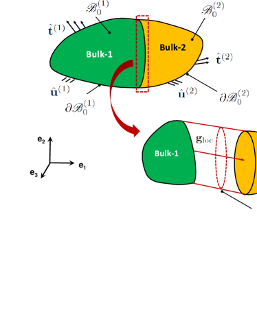
Figure 1: A schematic definition of two bodies separated by a cohesive interface.

The bodies undergo a motion $\boldsymbol{\phi}:\mathscr{B}_{0}\times[0,t]\rightarrow\mathscr{R}^{3}$, where $[0,t]$ is the time step interval, that maps the reference material points ($\mathbf{X}\in\mathscr{B}_{0}$) onto the current material points ($\mathbf{x}\in\mathscr{B}$), such that $\mathbf{x}=\boldsymbol{\phi}(\mathbf{X},t)$. The deformation gradient of the transformation is defined as $\mathbf{F}:=\partial_{\mathbf{X}}\phi(\mathbf{X},t)$, with the Jacobian $J=\text{det}[\mathbf{F}]$ and $\partial_{\mathbf{X}}$ denoting the partial derivative with respect to the reference frame. Moreover, it is supposed that the interface between both solids is characterized by the presence of a cohesive surface $S_{0}$.

Focusing our attention on the analysis of the interface between the solids, the contribution of the interface cohesive tractions $\mathbf{T}$, acting on $S_{0}$, to the Principle of Virtual Work of the mechanical system in the reference configuration is:

$$\Pi_{\mathrm{intf}}(\mathbf{g}_{\mathrm{loc}})=\int_{S_{0}}\mathbf{g}_{\mathrm{loc}}^{\mathrm{T}}\mathbf{T}\,\mathrm{d}S$$ (1)

where $\mathbf{g}_{\mathrm{loc}}$ is the gap vector accounting for opening and sliding displacements between the two sides of the interface. Note that, due to the geometrical nonlinearity, the traction vector previously defined corresponds to the nominal first Piola-Kirchhoff tractions related to the local basis of the interface in the reference configuration.

It is worth noting that in the large deformation setting, the gaps vector vanishes when the body undergoes rigid body motions, thus confirming the frame indifference of the formulation proposed in this paper.

The virtual variation of $\Pi_{\mathrm{intf}}$ according to the principle of virtual displacements reads:

$$\delta\Pi_{\mathrm{intf}}(\mathbf{g}_{\mathrm{loc}})= \int_{S_{0}}\left(\dfrac{\partial\mathbf{g}_{\mathrm{loc}}}{\partial\mathbf{u}}\delta\mathbf{u}\right)^{\mathrm{T}}\,\mathbf{T}\mathrm{d}S$$ (2)

$$= \delta\mathbf{u}^{\mathrm{T}}\int_{S_{0}}\left(\dfrac{\partial\mathbf{g}_{\mathrm{loc}}}{\partial\mathbf{u}}\right)^{\mathrm{T}}\,\mathbf{T}\mathrm{d}S$$

In case of large displacements, the updated coordinates of a generic point are given by $\mathbf{x}=\mathbf{X}+\mathbf{u}$, see Fig.2.

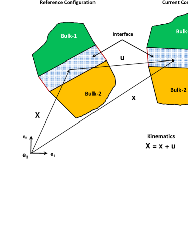
Figure 2: Kinematics definition of the interface along the deformation process.

As is generally proposed for interface formulations, it is convenient to define a middle line (in the 2D case) in the updated configuration by averaging the position vectors and the displacement fields of the upper and lower sides of the interface, see Fig.3 after performing a standard discretization process. Hence, the position vector $\overline{\mathbf{x}}$ of a generic point along this middle line can be determined by pre-multiplying the positioning vector $\mathbf{x}$ by an averaging operator $\mathbf{M}$:

$$\overline{\mathbf{x}}=\mathbf{M}\mathbf{x}$$ (3)

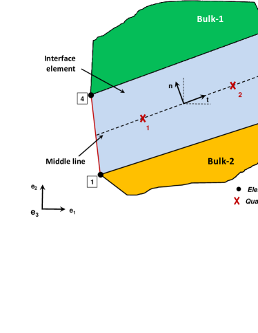
Figure 3: Sketch of the interface element with node numbering and integration points.

2.2 Finite element formulation

Based on isoparametric interpolation, the position vector at the interface can be approximated through:

$$\mathbf{x}\cong\overline{\mathbf{x}}^{e}=\mathbf{N}\mathbf{x}^{n}$$ (4)

where $\mathbf{x}^{n}$ denotes the nodal position vector (the superscript $n$ identifies nodal quantities), and $\mathbf{N}$ is the the operator that collects the shape functions and it depends on the natural coordinate of the element $\xi$. Introducing now the discretization of the interface into Eq.(3), the interpolated average position vector yields:

$$\overline{\mathbf{x}}\cong\overline{\mathbf{x}}^{e}=\mathbf{N}\mathbf{M}\mathbf{x}^{n}$$ (5)

Similarly, the coordinates of the points belonging to the middle line in the reference configuration, $\overline{\mathbf{X}}$, and their displacement vector, $\overline{\mathbf{u}}$, can be computed via a standard interpolation procedure from the nodal quantities

$$\overline{\mathbf{X}}\cong\overline{\mathbf{X}}^{e}=\mathbf{N}\mathbf{M}\mathbf{X}^{n},\quad\overline{\mathbf{u}}\cong\overline{\mathbf{u}}^{e}=\mathbf{N}\mathbf{M}\mathbf{d}$$ (6)

where $\mathbf{X}^{n}$ and $\mathbf{d}$ denote the position vector of the nodes in the reference configuration and their nodal displacement vector, respectively.

In 2D, the tangential and the normal vectors $\mathbf{t}$ and $\mathbf{n}$ to the middle line of the interface element used to define the local frame are given by:

$$\mathbf{t}=\dfrac{\partial\overline{\mathbf{x}}^{e}}{\partial\xi},\quad\mathbf{n}\cdot\mathbf{t}=0$$ (7)

Note that in 3D application, in line with the derivation proposed in Ortiz and Pandolfi OP99 , the convective tangential and normal vectors to the middle surface of the interface element ($\mathbf{t}_{1}$, $\mathbf{t}_{2}$ and $\mathbf{n}$) used to define the local frame are determined via differentiation of the average coordinates with respect to the natural coordinates $\xi$ and $\eta$:

$$\mathbf{t}_{1}=\dfrac{\partial\overline{\mathbf{x}}^{e}}{\partial\xi},\quad\mathbf{t}_{2}=\dfrac{\overline{\mathbf{x}}^{e}}{\partial\eta},\quad\mathbf{n}=\mathbf{t}_{1}\times\mathbf{t}_{2}$$ (8)

The gap vector in the reference cartesian frame, $\mathbf{g}$, can be obtained by pre-multiplying the nodal displacement vector $\mathbf{d}$ by a suitable operator $\mathbf{L}$ which provides the difference between the displacements of the upper and the lower bodies at the interface. Accordingly, within the FE discretization we have:

$$\mathbf{g}\cong\mathbf{g}^{e}=\mathbf{N}\mathbf{L}\mathbf{d}$$ (9)

The constitutive relation for the interface, i.e., the so-called cohesive zone model (CZM), is usually provided in a local frame defined by the normal and the tangential vectors to the average line of the interface element in order to distinguish between fracture Modes I and II, as introduced in Eq.(7). Therefore, the gap vector in this local frame, $\mathbf{g}_{\mathrm{loc}}$, has to be computed by multiplying the gap vector in the reference frame by a rotation operator $\mathbf{R}$:

$$\mathbf{g}_{\mathrm{loc}}=\mathbf{R}(\mathbf{u})\mathbf{g}$$ (10)

It is remarkable to note that, in case of large displacements, the operator $\mathbf{R}(\mathbf{u})$ is a function of the displacement field. Its expression is detailed in Section 4 for the 2D case that represents the main scope of the present work (the 3D version can be derived adapting the formulation here developed). Consequently, a consistent formulation must take into account this dependency in the subsequent linearization of the discretized version of the interface contribution to the Principle of Virtual Work within the classical Newton-Raphson iterative solution scheme. This dependency will lead to the so-called geometric contribution to the element stiffness matrix. Introducing the FE discretization, Eq.(10) can be rewritten as:

$$\mathbf{g}_{\mathrm{loc}}^{e}=\mathbf{R}(\mathbf{d})\mathbf{N}\mathbf{L}\mathbf{d}$$ (11)

Examining the terms entering the virtual variation of the virtual work in Eq.(2), the partial derivative $(\partial\mathbf{g}_{\mathrm{loc}}/\partial\mathbf{u})$ is approximated by:

$$\dfrac{\partial\mathbf{g}_{\mathrm{loc}}}{\partial\mathbf{u}}\cong\dfrac{\partial\mathbf{g}_{\mathrm{loc}}^{e}}{\partial\mathbf{d}}=\mathbf{R}(\mathbf{d})\mathbf{N}\mathbf{L}+\dfrac{\partial\mathbf{R}(\mathbf{d})}{\partial\mathbf{d}}\mathbf{N}\mathbf{L}\mathbf{d}$$ (12)

where the differentiation of the second order tensor $\mathbf{R}$ with respect to the components of the vector $\mathbf{d}$ leads to a third order tensor. Note that in (12) the formulation is simplified by omitting the second derivative of the rotation matrix with respect to the displacement vector. This vanishes in case of linear displacement interpolation under the assumption that the norm of the tangent vector $\mathbf{t}$ does not depend on the displacement field. In this regard, we also assessed the role of this term based on representative numerical tests adopting alternative interpolation schemes. It was found that this term has an almost negligible effect on the results and it is therefore reasonable to be neglected.

The operator $\mathbf{B}=\mathbf{N}\mathbf{L}$ is now introduced and Eq.(12) can be rephrased as:

$$\dfrac{\partial\mathbf{g}_{\mathrm{loc}}^{e}}{\partial\mathbf{d}}=\mathbf{R}\mathbf{B}+\dfrac{\partial\mathbf{R}}{\partial\mathbf{d}}\mathbf{B}\mathbf{d}$$ (13)

The matrices $\mathbf{R}$ and $\mathbf{B}$ are evaluated at the element level, though the typical superscript ($e$) has been omitted here to simplify notation.

Inserting this intermediate result into the discretized version of Eq.(2), where $\mathbf{u}$ is simply replaced by $\mathbf{d}$, the following general formulation valid for any kind of interface element topology dealing with geometric and material nonlinearities is derived:

$$\delta\Pi_{\mathrm{intf}}^{e}=\delta\mathbf{d}^{\mathrm{T}}\int_{S_{0}}\left(\mathbf{R}\mathbf{B}+\dfrac{\partial\mathbf{R}}{\partial\mathbf{d}}\mathbf{B}\mathbf{d}\right)^{\mathrm{T}}\mathbf{T}\,\mathrm{d}S$$ (14)

The solution of the variational equation $\delta\Pi_{\mathrm{intf}}^{e}=\delta\mathbf{d}^{\mathrm{T}}\mathbf{f}_{\mathrm{intf}}^{e}=0$ $\forall\delta\mathbf{d}$ results in the equations set $\mathbf{f}_{\mathrm{intf}}^{e}=0$, where $\mathbf{f}_{\mathrm{intf}}^{e}$ is a nonlinear function of the unknown $\mathbf{d}$ and assumes the role of the residual vector in the Newton-Raphson iterative scheme:

$$\mathbf{f}^{e,k}_{\mathrm{intf}}=\int_{S_{0}}\left(\mathbf{R}\mathbf{B}+\dfrac{\partial\mathbf{R}}{\partial\mathbf{d}}\mathbf{B}\mathbf{d}\right)^{\mathrm{T}}\mathbf{T}\,\mathrm{d}S$$ (15)

which leads to the following equations set for the computation of the corrector $\Delta\mathbf{d}$ at each iteration $k$:

$$\mathbf{K}^{e,k}\Delta\mathbf{d} =-\mathbf{f}_{\mathrm{intf}}^{e,k}$$ (16a)

$$\mathbf{d}^{k+1} =\mathbf{d}^{k}+\Delta\mathbf{d}$$ (16b)

To alleviate the notation, the superscript $k$ will be omitted in the sequel. Following standard arguments of nonlinear FE formulations, the element stiffness matrix $\mathbf{K}^{e}$ is obtained from the linearization of the residual, i.e., $\mathbf{K}^{e}=\partial\mathbf{f}_{\mathrm{intf}}/\partial\mathbf{d}$ and it is evaluated by using the displacement field solution at the iteration $k$:

$$\mathbf{K}^{e}= \int_{S_{0}}\left[2\mathbf{B}^{\mathrm{T}}\dfrac{\partial\mathbf{R}^{\mathrm{T}}}{\partial\mathbf{d}}\mathbf{T}\right.$$ (17)

$$\left.+\left(\mathbf{B}^{\mathrm{T}}\mathbf{R}^{\mathrm{T}}+\mathbf{d}^{\mathrm{T}}\mathbf{B}^{\mathrm{T}}\dfrac{\partial\mathbf{R}^{\mathrm{T}}}{\partial\mathbf{d}}\right)\dfrac{\partial\mathbf{T}}{\partial\mathbf{d}}\right]\,\mathrm{d}S$$

In this derivation, as it was already stated, the second-order differentiation of the rotation matrix $\mathbf{R}$ was omitted.

The derivative of the cohesive traction vector $\mathbf{T}$ with respect to the displacement vector $\mathbf{d}$ can be determined via a chain rule differentiation:

$$\dfrac{\partial\mathbf{T}}{\partial\mathbf{d}}=\dfrac{\partial\mathbf{T}}{\partial\mathbf{g}_{\mathrm{loc}}}\dfrac{\mathbf{g}_{\mathrm{loc}}}{\partial\mathbf{d}}=\mathbf{C}\left(\mathbf{R}\mathbf{B}+\dfrac{\partial\mathbf{R}}{\partial\mathbf{d}}\mathbf{B}\mathbf{d}\right)$$ (18)

where $\mathbf{C}=\dfrac{\partial\mathbf{T}}{\partial\mathbf{g}_{\mathrm{loc}}}$ represents the tangent interface constitutive matrix whose expression will be detailed in the next section.

After some algebra we obtain the following result:

$$\mathbf{K}^{e}= \int_{S_{0}}\mathbf{B}^{\mathrm{T}}\mathbf{R}^{\mathrm{T}}\mathbf{C}\mathbf{R}\mathbf{B}\,\mathrm{d}S$$ (19)

$$+\int_{S_{0}}\left[2\mathbf{B}^{\mathrm{T}}\dfrac{\partial\mathbf{R}^{\mathrm{T}}}{\partial\mathbf{d}}\mathbf{T}+\mathbf{d}^{\mathrm{T}}\mathbf{B}^{\mathrm{T}}\dfrac{\partial\mathbf{R}^{\mathrm{T}}}{\partial\mathbf{d}}\mathbf{C}\dfrac{\partial\mathbf{R}}{\partial\mathbf{d}}\mathbf{B}\mathbf{d}\right.$$

$$\left.+\mathbf{B}^{\mathrm{T}}\mathbf{R}^{\mathrm{T}}\mathbf{C}\dfrac{\partial\mathbf{R}}{\partial\mathbf{d}}\mathbf{B}\mathbf{d}+\mathbf{d}^{\mathrm{T}}\mathbf{B}^{\mathrm{T}}\dfrac{\partial\mathbf{R}^{\mathrm{T}}}{\partial\mathbf{d}}\mathbf{C}\mathbf{R}\mathbf{B}\right]\,\mathrm{d}S$$

Summarizing, the tangent stiffness matrix which accounts for both the material and the geometric contributions reads:

$$\mathbf{K}^{e}=\mathbf{K}^{e}_{\mathrm{mat}}+\mathbf{K}^{e}_{\mathrm{geom}}$$ (20a)

$$\mathbf{K}^{e}_{\mathrm{mat}}=\int_{S_{0}}\mathbf{B}^{\mathrm{T}}\mathbf{R}^{\mathrm{T}}\mathbf{C}\mathbf{R}\mathbf{B}\,\mathrm{d}S$$ (20b)

$$\mathbf{K}^{e}_{\mathrm{geom}}=\int_{S_{0}}\left[2\mathbf{B}^{\mathrm{T}}\dfrac{\partial\mathbf{R}^{\mathrm{T}}}{\partial\mathbf{d}}\mathbf{T}+\mathbf{d}^{\mathrm{T}}\mathbf{B}^{\mathrm{T}}\dfrac{\partial\mathbf{R}^{\mathrm{T}}}{\partial\mathbf{d}}\mathbf{C}\dfrac{\partial\mathbf{R}}{\partial\mathbf{d}}\mathbf{B}\mathbf{d}\right.$$

$$\left.+\left(\mathbf{B}^{\mathrm{T}}\mathbf{R}^{\mathrm{T}}\mathbf{C}\dfrac{\partial\mathbf{R}}{\partial\mathbf{d}}\mathbf{B}\mathbf{d}+\mathbf{d}^{\mathrm{T}}\mathbf{B}^{\mathrm{T}}\dfrac{\partial\mathbf{R}^{\mathrm{T}}}{\partial\mathbf{d}}\mathbf{C}\mathbf{R}\mathbf{B}\right)\right]\,\mathrm{d}S$$ (20c)

In case of small displacements, Eq.(20) reduces to the standard form of the material contribution to the element stiffness matrix, Eq.(20b). In case of large displacements, the complete tangent stiffness matrix is composed of four terms, see Eq.(20c). Only the first one, involving the computation of the cohesive traction vector $\mathbf{T}$ is not symmetric. Therefore, a nonsymmetric solver has to be used. However, in case of a symmetric constitutive matrix $\mathbf{C}$ for the interface, as it happens in case of the same CZM parameters for Mode I and Mode II, we explored the possibility to neglect the non symmetric contribution to $\mathbf{K}_{g}$. The examples discussed in Section 5 will show that this will not affect the accuracy of the solution and slightly penalize the convergence rate. The omission of this term, on the other hand, makes it possible the use of symmetric solvers. This fact represents an obvious advantage in case of massive computations.

3 Material models

With reference to the continuum, to assess the effect of large displacements on debonding of thin structures, both a small deformation and a large deformation versions of a standard homogeneous isotropic hyperelastic material model are considered in the sequel. The derivation is here omitted for the sake of brevity. The readers can refer to FEAP for more details.

Regarding the cohesive traction vector $\mathbf{T}$, with the aim of quantifying the role of the geometric nonlinear effects along the decohesion process, two different types of interface constitutive laws are examined.

First, a tension cut-off CZM is considered, with uncoupled Mode I and Mode II deformation. This type of CZM has the advantage of allowing for closed form solutions for specific testing configurations, like for the double cantilever beam test WH . The stiffness of the CZM can be related to the Young’s modulus $E$ and to the thickness of the adhesive $h$, i.e. $k=\sigma_{\max}/l_{\text{nc}}\sim E/h$ where $\sigma_{\max}$ and $l_{\text{nc}}$ denote the critical traction for damage initiation and the critical relative displacement, respectively. In this approach, when the crack sliding or opening displacements overcome a critical value corresponding to the achievement of the adhesive strength, $\sigma_{\max}$, the interface suddenly debonds. Since such critical relative displacements for failure are very small quantities in applications, the process zone size is expected to be quite small and limited within a region very close to the real crack tip, where displacements are moderately small.

The cohesive traction vector $\mathbf{T}=(\tau,\sigma)^{\mathrm{T}}$ reads:

$$\tau= \tau_{\max}\dfrac{g_{\mathrm{loc,t}}}{l_{\text{tc}}}$$ (21a)

$$\sigma= \sigma_{\max}\dfrac{g_{\mathrm{loc,n}}}{l_{\text{nc}}}$$ (21b)

where $g_{\mathrm{loc,t}}$ and $g_{\mathrm{loc,n}}$ are the tangential and normal components of the gap vector $\mathbf{g}_{\mathrm{loc}}$, whereas $l_{\text{tc}}$ and $l_{\text{nc}}$ are the critical sliding and opening displacements. The tangent constitutive matrix stemming from the linearization of the CZM tractions with respect to the gap vector is:

$$\mathbf{C}=\left[\begin{array}[]{cc}\dfrac{\tau_{\max}}{l_{\text{tc}}}&0\\ 0&\dfrac{\sigma_{\max}}{l_{\text{nc}}}\\ \end{array}\right]$$ (22)

In this case, in line with the previous arguments, the resulting interface element stiffness matrix is always symmetric.

As second formulation, we consider the polynomial CZM by Tvergaard TV as an example of an interface constitutive relation where the cohesive traction vector $\mathbf{T}=(\tau,\sigma)^{\mathrm{T}}$ is a nonlinear function of the sliding and opening displacements with a softening branch after reaching the maximum cohesive tractions. For the same values of the parameters $\tau_{\max}$, $\sigma_{\max}$ and of the initial stiffness as for the tension cut-off model, this CZM has a larger fracture energy and therefore a more widespread process zone is expected. In this model, the cohesive tractions are given by

$$\tau= \tau_{\max}\dfrac{g_{\mathrm{loc},t}}{l_{\text{tc}}}P(\lambda)$$ (23a)

$$\sigma= \sigma_{\max}\dfrac{g_{\mathrm{loc},n}}{l_{\text{nc}}}P(\lambda)$$ (23b)

where

$$P(\lambda)= \left\{\begin{array}[]{ll}\dfrac{27}{4}\left(1-2\lambda+\lambda^{2}\right),&\text{for}\,0\leq\lambda\leq 1\\ 0,&\text{otherwise}\end{array}\right.$$ (24c)

$$\lambda= \sqrt{\left(\dfrac{g_{\mathrm{loc},n}}{l_{\mathrm{nc}}}\right)^{2}+\left(\dfrac{g_{\mathrm{loc},t}}{l_{\mathrm{tc}}}\right)^{2}}$$ (24d)

For this CZM, the tangent constitutive matrix reads:

$$\mathbf{C}= \left[\begin{array}[]{c}\tau_{\max}\dfrac{P}{l_{\mathrm{tc}}}+\tau_{\max}\dfrac{g_{\mathrm{loc},t}}{l_{\mathrm{tc}}}\dfrac{\partial P}{\partial\lambda}\dfrac{\partial\lambda}{\partial g_{\mathrm{loc},t}}\\ \tau_{\max}\dfrac{g_{\mathrm{loc},t}}{l_{\mathrm{tc}}}\dfrac{\partial P}{\partial\lambda}\dfrac{\partial\lambda}{\partial g_{\mathrm{loc},n}}\end{array}\right.$$ (25)

$$\left.\begin{array}[]{c}\sigma_{\max}\dfrac{g_{\mathrm{loc},n}}{l_{\mathrm{nc}}}\dfrac{\partial P}{\partial\lambda}\dfrac{\partial\lambda}{\partial g_{\mathrm{loc},t}}\\ \sigma_{\max}\dfrac{P}{l_{\mathrm{nc}}}+\sigma_{\max}\dfrac{g_{\mathrm{loc},n}}{l_{\mathrm{nc}}}\dfrac{\partial P}{\partial\lambda}\dfrac{\partial\lambda}{\partial g_{\mathrm{loc},n}}\end{array}\right]$$

4 Matrix operators for finite element implementation

This section covers the main features concerning the numerical implementation of the large displacement interface element formulation proposed in the previous section. According to the derivation presented in Section 2, we restrict our attention to the implementation of the element in a 2D version, although Eqs.(18) and (19) are the same for 3D problems, provided that a middle surface is introduced in analogy with the middle line for the 2D case.

Let us to consider a 4 node bilinear interface element, see Fig.3. The corresponding shape functions to accomplish the numerical integration are $N_{1}=\dfrac{1}{2}(1-\xi)$ and $N_{2}=\dfrac{1}{2}(1+\xi)$. Each node has two degrees of freedom, so that the nodal position and displacement vectors are arranged as:

$$\mathbf{X} =(X_{1},Y_{1},X_{2},Y_{2},X_{3},Y_{3},X_{4},Y_{4})^{\mathrm{T}}$$ (26a)

$$\mathbf{d} =(u_{1},v_{1},u_{2},v_{2},u_{3},v_{3},u_{4},v_{4})^{\mathrm{T}}$$ (26b)

where $X_{i}$, $Y_{i}$ identifies the cartesian coordinates corresponding to the node $i$ and $u_{i}$ and $v_{i}$ stands for the corresponding displacements along the $X$ and $Y$ directions.

The gap and the traction vectors that characterizes the CZM are evaluated in correspondence of each integration point, so that:

$$\mathbf{g}_{\mathrm{loc}} =(g_{\mathrm{loc,t}},g_{\mathrm{loc,n}})^{\mathrm{T}}$$ (27a)

$$\mathbf{T} =(\tau,\sigma)^{\mathrm{T}}$$ (27b)

Next, the matrix operators defined in Section 2 to determine the coordinates and the gaps of the points belonging to the interface middle line take the form:

$$\mathbf{N} =\left[\begin{array}[]{cc}N_{1}\mathbf{I}&N_{2}\mathbf{I}\end{array}\right]$$ (28b)

$$\mathbf{M} =\dfrac{1}{2}\left[\begin{array}[]{cccc}\mathbf{I}&\mathbf{0}&\mathbf{0}&\mathbf{I}\\ \mathbf{0}&\mathbf{I}&\mathbf{I}&\mathbf{0}\\ \end{array}\right]\quad\mathbf{L}=\left[\begin{array}[]{cccc}-\mathbf{I}&\mathbf{0}&\mathbf{0}&\mathbf{I}\\ \mathbf{0}&-\mathbf{I}&\mathbf{I}&\mathbf{0}\\ \end{array}\right]$$ (28g)

where $\mathbf{0}$ is a $2\times 2$ null matrix and $\mathbf{I}$ is a $2\times 2$ identity matrix. As previously stated, the CMZ is evaluated at the local reference system that is defined by the tangential vector $\mathbf{t}$ and the normal vector $\mathbf{n}$ to this middle line. Thus, the rotation operator yields:

$$\mathbf{R}=\left[\begin{array}[]{cc}t_{x}&t_{y}\\ n_{x}&n_{y}\\ \end{array}\right]$$ (29)

where:

$$t_{x} =n_{y}=\dfrac{X_{2}+u_{2}+X_{3}+u_{3}-X_{1}-u_{1}-X_{4}-u_{4}}{2\|\mathbf{t}\|}$$

$$t_{y} =-n_{x}=\dfrac{Y_{2}+v_{2}+Y_{3}+v_{3}-Y_{1}-v_{1}-Y_{4}-v_{4}}{2\|\mathbf{t}\|}$$

and the symbol $\|.\|$ denotes the Euclidean norm of the corresponding vector. Note that, differing from previous interface formulations PW11b , this operator is evaluated at each integration point at the element level.

The operator stemming from the third order tensor has to be computed with care. For the present particular case it renders:

$$\dfrac{\partial\mathbf{R}}{\partial\mathbf{d}}\mathbf{B}\mathbf{d}=\left[\begin{array}[]{cccccccc}-a&-b&+a&+b&+a&+b&-a&-b\\ -b&+a&+b&-a&+b&-a&-b&+a\\ \end{array}\right]$$ (30)

where $a=\dfrac{-N_{1}u_{1}-N_{2}u_{2}+N_{2}u_{3}+N_{1}u_{4}}{2\|\mathbf{t}\|}$ and $b=\dfrac{-N_{1}v_{1}-N_{2}v_{2}+N_{2}v_{3}+N_{1}v_{4}}{2\|\mathbf{t}\|}$.

The remaining operations to accomplish are straightforward, and therefore are omitted here for the sake of conciseness.

The algorithmic treatment of the proposed formulation, implemented by the present authors both in the Finite Element Analysis Program FEAP and in the commercial software Abaqus as user defined subroutines, is summarized in the following sequence of main operations, see Algorithm 1. Note that the external loop over $j$ refers to the numerical integration, whereas the variable $nlgeom$ indicates a flag defined in the input file to select between: (i) small displacement formulation ($nlgeom=0$) or (ii) large displacement formulation ($nlgeom=1$).

Data: Given: $\mathbf{X}^{e}$, $\mathbf{d}$, $\Delta\mathbf{d}$, $\Delta t$

if nlgeom $>0$ then

       Update the geometry: $\mathbf{x}^{e}=\mathbf{X}^{e}+\mathbf{d}$;

      

else

       $\mathbf{x}^{e}=\mathbf{X}^{e}$;

      

end if

Construct $\mathbf{L}$;

Loop over the integration points;

for $j=1$ to $2$  do

       Evaluate shape functions and derivatives;

       Compute the local basis vectors $[\mathbf{t},\mathbf{n}]$ and rotation matrix $\mathbf{R}$;

       Construct $\mathbf{N}$;

       Perform $\mathbf{B}=\mathbf{N}\mathbf{L}$;

       Compute $\mathbf{R}\mathbf{B}$ $\rightarrow$ $(\mathbf{R}\mathbf{B})^{T}$;

       Evaluate $\mathbf{T}$, $\mathbf{C}$ according to the selected CZM;

end for

if nlgeom $>0$ then

      Perform: $\frac{\partial\mathbf{R}}{\partial\mathbf{d}}\mathbf{B}\mathbf{d}$;

       Construct the geometrical stiffness matrix $\mathbf{K}_{\mathrm{geom}}^{e}$, Eq.(20c);

       Compute the geometric part of the residual vector $\mathbf{f}_{\mathrm{intf}}^{e}$, second term of Eq.(15);

else

      Compute the material part of the residual vector $\mathbf{f}_{\mathrm{intf}}^{e}$,first term of Eq.(15);

end if

Evaluate the material contribution to the stiffness matrix $\mathbf{K}_{\mathrm{mat}}^{e}$, Eq.(20b);

if nlgeom $>0$ then

      $\mathbf{K}^{e}=\mathbf{K}_{\mathrm{mat}}^{e}+\mathbf{K}_{\mathrm{geom}}^{e}$

else

       $\mathbf{K}^{e}=\mathbf{K}_{\mathrm{mat}}^{e}$

end if

Update stiffness matrix and r.h.s. vector;

Algorithm 1 Numerical implementation of the large displacement interface element.

5 Numerical examples

In this section, the numerical performance of the proposed element is illustrated. To this aim, two applications are selected. First, we investigate the element capabilities through a series of benchmark problems to highlight the principal capabilities that the present element formulation incorporates. Second, a structural application consisting of a peeling test is addressed. Small or finite displacement formulations for the continuum and for the interface element are examined, along with two different CZM formulations.

5.1 Benchmark tests

A preliminary test problem shown in Fig.4(a) is analyzed in order to assess the performance of the new interface element for large displacements as compared to a standard formulation for small displacement. This benchmark problem aims at investigating the interplay between geometric and material nonlinearities, an issue not yet rigorously quantified in the related literature. Therefore, as was previously stated, we consider small or large deformation hyperelastic material models for the continuum in order to investigate the role played by the different interface element formulations in these two cases. Hence, each numerical test will be identified by labels $X-Y(Z)$. Whereas $X$ refers to the interface element formulation and it can be $S$ or $L$ depending on the small or the large displacement formulation used, the second label $Y$ stands for the constitutive model of the continuum and again it can be $S$ or $L$ depending on the small or large deformation theory adopted for the hyperelastic material. The symbol $Z$ in parenthesis denotes the solver used ($s$ for symmetric solver or $u$ for a non symmetric solver).

In this benchmark problem, two blocks of lateral size 1 mm and different heights are discretized by a single finite element each. The lower block of unit height has a Young’s modulus $E_{1}=500$ MPa in order to simulate an almost rigid substrate, whereas the upper block has a height of 0.1 mm and a Young modulus $E_{2}=5$ MPa to simulate a highly deformable elastomeric tape or a paper sheet. Both materials have a vanishing Poisson’s ratio and the simulations are conducted under plane strain assumption. An interface element is placed between the two blocks and its CZM can have either a tension cut-off or a polynomial form, see Fig.4(b) for the Mode I relations (Section 3). The values of the CZM parameters $\sigma_{\max}$ and $\tau_{\max}$ are selected the same for both the tension cut-off and the polynomial CZMs, to perform a consistent comparison. On the other hand, the fracture energy of the tension cut-off model is much smaller than that of the polynomial CZM, as it can be readily visualized in Fig.4(b) from the different area under the respective traction-separation relations. The value of $l_{\mathrm{nc}}$ in the tension cut-off model has been selected so that the tension cut-off curve is tangent to the polynomial CZM at $g_{\mathrm{loc,n}}=0$.

As far as the boundary conditions are concerned, a non-uniform Mixed Mode debonding problem is simulated by restraining the first block at the basis and imposing a linear vertical displacement variation to the upper side of the second block. This testing configuration has been chosen because leads to large displacements at the interface during the deformation process and therefore Mode Mixity OR . In other types of loading, such as uniform Mode I debonding, uniform Mode II debonding or uniform Mixed Mode debonding, the response of the interface element would be in fact the same regardless of the small or large displacement formulation used, since the orientation of the local frame does not change during the deformation process. These trends are consistent with the results reported in BSG07 , although they were based on an approximated large displacement formulation for the interface element deduced by the kinematics of a beam element in large displacements and rotations.

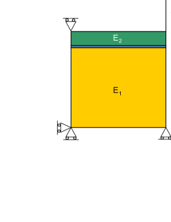
(a) Sketch of the test problem

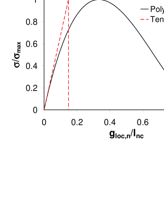
(b) $\sigma/\sigma{\max}$ vs. $g_{\mathrm{loc,n}}$

Figure 4: Sketch of the geometry of the 2-blocks Mixed Mode test problem and illustration of the normal cohesive traction-normal gap CZM relations used in the simulations.

The vertical reaction force $F$ in the constrained node is plotted vs. the imposed displacement $\Delta$ in Fig.5 for an interface tougher in Mode I than in Mode II, i.e., with $\sigma_{\max}/\tau_{\max}=10$ and $l_{\mathrm{nc}}=l_{\mathrm{tc}}=0.1$ mm. The results for the tension cut-off CZM are shown in Fig.5(a) and those for the polynomial CZM are depicted in Fig.5(b). Examining the curves related to the tension cut-off CZM, Fig.5(a), we note that, in case of the small deformation theory for the continuum, curves labeled $(S-S)$ and $(L-S)$ are almost coincident before the peak load, i.e., before complete debonding of the first Gauss point of the interface. Note that the labels $(s)$ and $(u)$ make reference to the symmetric or unsymmetric character of the formulation. In this sense, the small-displacement case always leads to a symmetric stiffness matrix, whereas the large displacement case provides a general unsymmetric formulation, in which the role of the term that break the symmetry (see Eq.(20c)) is examined.

After the peak load, an abrupt reduction in the interface load-carrying capacity takes place and the structural response is characterized by a lower stiffness until complete decohesion takes place. In this respect, the large displacement formulation for the interface predicts a much lower displacement jump for complete debonding. A similar difference can be noticed in case of a large deformation formulation for the continuum, see curves labeled $(S-L)$ and $(L-L)$. Since this CZM does not consider coupling between Mode I and Mode II, i.e., the matrix $\mathbf{C}$ is diagonal, it makes sense to compare the results for the large displacements interface element formulation by considering the complete expression of the tangent stiffness matrix and using a non symmetric solver or the approximate symmetric expression and using a symmetric solver. As it can be seen from Fig.5(a), the results are coincident.

In case of the polynomial CZM, the results have the same trend as for the tension cut-off, just with much smoother curves during the debonding process. In light of the previous arguments, it is worth noting that for a given assumption regarding the kinematics of the continuum, the use of a large displacement formulation for the interface instead of its small displacement counterpart has a predominant effect on the softening branch of the $F-\Delta$ response. In this case, since the matrix $\mathbf{C}$ is not symmetric due to the expression of the CZM, a non symmetric solver has been always used and the full expression for the geometric stiffness matrix has been retained in the computations.

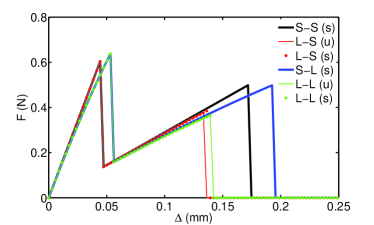
(a) Tension cut-off CZM

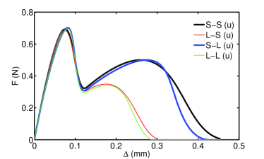
(b) Polynomial CZM

Figure 5: Total force vs. imposed displacement for the test problem in Fig.4(a) and different CZM formulations for an interface tougher in Mode I than in Mode II ($\sigma_{\max}/\tau_{\max}=10$). $(S-S)$: small displacement interface element & small deformation continuum; $(L-S)$: large displacement interface element & small deformation continuum; $(S-L)$: small displacement interface element & large deformation continuum; $(L-L)$: large displacement interface element & large deformation continuum.

Examining the element performance in case of an interface with the same fracture parameters in Mode I and in Mode II ($\sigma_{\max}/\tau_{\max}=1$), see Fig.6, we find that the discrepancy between the predictions in case of large or small interface element formulations are minimal. On the other hand, small or large displacement formulations for the continuum significantly affects the post-peak branch. Since in this case the matrix $\mathbf{C}$ is symmetric for both the CZM formulations, the use of the complete non symmetric tangent stiffness matrix or its symmetric version by neglecting the non symmetric contribution to its geometric component have been compared and the results are again coincident.

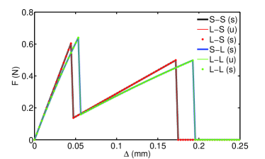
(a) Tension cut-off CZM

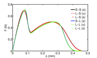
(b) Polynomial CZM

Figure 6: Total force vs. imposed displacement for the test problem in Fig.4(a) and different CZM formulations for an interface with the same toughness in Mode I and in Mode II ($\sigma_{\max}/\tau_{\max}=1$). $(S-S)$: small displacement interface element & small deformation continuum; $(L-S)$: large displacement interface element & small deformation continuum; $(S-L)$: small displacement interface element & large deformation continuum; $(L-L)$: large displacement interface element & large deformation continuum.

Finally, the last scenario to be inspected is represented by the case of an interface much tougher in Mode II than in Mode I ($\sigma_{\max}/\tau_{\max}=0.1$), see Fig.7. As far as the choice of the symmetric or the non symmetric solver is concerned, the same comments to the case when Mode I prevails over Mode II apply. In this instance, since the loading test is predominantly in Mode I, we observe a much lower peeling force $F$ in this benchmark test. Additionally, slight discrepancies between the numerical predictions using large or small interface element formulations are noticed.

Therefore, it is possible to draw the practical conclusion that the large displacement formulation for the interface should be primarily used in case of applications with $\sigma_{\max}>\tau_{\max}$, as, e.g., in fibrilation problems where the shear strength of cellulose or polymeric fibrils is almost negligible as compared to their axial strength.

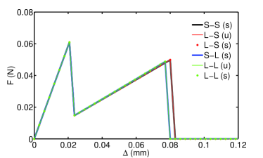
(a) Tension cut-off CZM

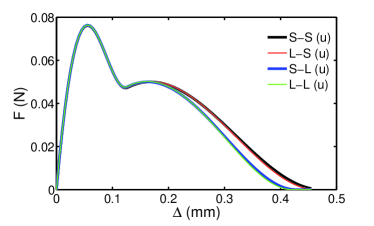
(b) Polynomial CZM

Figure 7: Total force vs. imposed displacement for the test problem in Fig.4(a) and different CZM formulations for an interface tougher in Mode II than in Mode I ($\sigma_{\max}/\tau_{\max}=0.1$). $(S-S)$: small displacement interface element & small deformation continuum; $(L-S)$: large displacement interface element & small deformation continuum; $(S-L)$: small displacement interface element & large deformation continuum; $(L-L)$: large displacement interface element & large deformation continuum.

5.2 Structural application: peeling test and comparison with experiments

Examining now a structural problem where the large displacement formulation for the interface element is deemed to be crucial, a peeling test where a thin layer is pulled from al almost rigid substrate by the action of a vertical displacement imposed to the top right corner is considered (see the final deformed shapes in case of $(S-S)$ or $(L-L)$ formulations in Fig.8). The material parameters for the bulks and for the CZMs (tension cut-off and polynomial CZMs) are the same as in the previous example, considering the case of an interface tougher in Mode I than in Mode II ($\sigma_{\max}/\tau_{\max}=10$, where the large displacement formulation for the interface element was found to significantly differ from the small displacement one. A non symmetric solver and the complete expression for the tangent stiffness matrix are used.

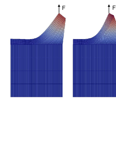
Figure 8: Deformed meshes of the peeling test in case of small displacement formulations for the continuum and the interface element (left, $(S-S)$) or large displacement formulations (right, $(L-L)$).

The force-displacement curves for different kinematics formulations are compared in Fig.9. As a general trend, the large displacement formulation for the interface element leads to lower peak loads as compared to its small displacement counterpart, for a given kinematical model of the continuum. Large differences among the predictions of the formulations can also be observed as far as the softening branches are concerned.

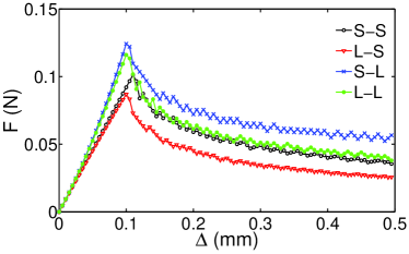
(a) Tension cut-off CZM

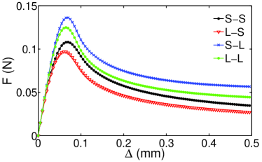
(b) Polynomial CZM

Figure 9: Total force vs. imposed displacement for the peeling test in Fig.7 and different CZM formulations for an interface tougher in Mode I than in Mode II ($\sigma_{\max}/\tau_{\max}=10$)). $(S-S)$: small displacement interface element & small deformation continuum; $(L-S)$: large displacement interface element & small deformation continuum; $(S-L)$: small displacement interface element & large deformation continuum; $(L-L)$: large displacement interface element & large deformation continuum.

Additionally, some comments on the convergence of the formulation herein proposed have to be added. First, from the numerical point of view, the interface element formulation was found to be quite stable, with the appearance of small oscillations in the softening branches for the peeling test only in case of the tension cut-off CZM. These effects are caused by the sharp discontinuity in the traction-gap constitutive relation leading to small jumps in the load when debonding takes place in a given Gauss point, see Figs.9(a). These small oscillations disappear in case of the polynomial CZM, since a softening is included in the interface constitutive relation.

Second, for the sake of completeness, the mesh convergence of the method is tested by considering the polynomial CZM and performing peeling tests as in Fig.9(b) for the (L-L) case, with different mesh refinement for the bulk and the interface in the horizontal direction. In the coarsest discretization (mesh 1), only 25 elements along the interface are used. Finer meshes with 50 elements (mesh 2), 100 elements (mesh 3) and 200 elements (mesh 4) along the interface are also considered. The corresponding load-displacement curves are shown in Fig.10, where an excellent mesh-independency even for the coarsest mesh can be observed.

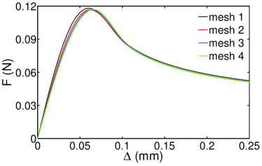
Figure 10: Mesh convergence study for the peeling test in Fig.8. Mesh 1 corresponds to 25 elements along the interface, mesh 2 to 50 elements, mesh 3 to 100 elements and mesh 4 to 200 elements.

The predictive capabilities of the proposed formulation are finally checked against experimental results. To this aim, a $90^{\circ}$ peeling of a backsheet (0.1 mm thick, Young’s modulus 2.8 GPa, vanishing Poisson’s ratio, hyperelastic material) from a glass substrate (4 mm thick, Young’s modulus 73 GPa, vanishing Poisson’s ratio, linear elastic material) is simulated by modelling the adhesive response of the Epoxy Vynil Acetate (EVA) interlayer via the polynomial CZM used in the previous examples. The parameters to be identified are the peak cohesive traction $\sigma_{\max}$ and the fracture energy $G_{\mathrm{Ic}}$, which is proportional to the critical opening displacement $l_{\mathrm{nc}}$. The same parameters for Mode I and Mode II deformation are used and the symmetric formulation of the interface element for large displacement analyses is adopted. The test is conducted under plane strain conditions. Mesh and boundary conditions are analogous to those displayed in Fig.8, although the upper layer is much thinner in the present problem. Four finite elements are used to discretize the backsheet through its thickness and 200 finite elements are used along the interface, considering an initial bonded length of 50 mm.

For this test, essential to ascertain the reliability of backsheet bonding in photovoltaic systems, experimental results are reported in solmat . Since the material parameters and the exact dimensions corresponding to the experimental force-peel extension curve are not listed in solmat , we use values conforming to the standard materials used in PV production, see JSA . Another source of uncertainty regards the way the peeling extension is measured, since no details are provided in solmat . In the numerical simulation we predict the peeling extension via the location of the fictitious crack tip position. Keeping in mind that, alternatively, the position of the real crack tip could be used, this choice makes a certain difference especially in the pre-peak branch of the force-peel extension curve.

Numerical results are shown in Fig.11 for $G_{\mathrm{Ic}}=5.4$ N/mm, which corresponds to the steady-state peeling force measured in experiments. A series of curves obtained by varying $\sigma_{\max}$ in the range from 3.6 to 28.8 N/mm are displayed and are used to identify the value of $\sigma_{\max}$ which provides the best agreement with experiments. In the present case, we found $\sigma_{\max}\sim 5.8$ N/mm, corresponding to the black dashed curve in Fig.11. The numerical methods is able to predict the stead-state peeling force very well, in excellent agreement with experiments. The pre-peak response, which has the highest degree of inaccuracy in the real tests, is in any case reasonably well reproduced.

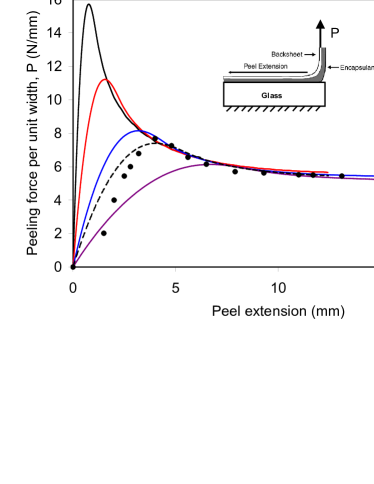
Figure 11: Peeling of a backsheet from a glass substrate: numerical vs. experimental results taken from solmat .

6 Conclusions and outlook

In this paper, a consistent derivation of an interface element for large displacements applications has been proposed.

The present theory finds its variational basis in the interface contribution to the Principle of Virtual Work of the whole mechanical system. Our present work, differing from alternative formulations presented in the literature, furnishes a consistent derivation of the interface model involving large deformations. Particularly, the cohesive model herein developed takes into account the full finite kinematics in which the material and the geometrical contributions to the element stiffness matrix are clearly determined.

The corresponding finite element discretization of the interface model has been accomplished based on a linear two-dimensional zero-thickness interface element for which the fundamental operators and the implementation details have been addressed. The compact and consistent theoretical derivation allows its straightforward generalization to different orders of the kinematic interpolation and to 3D topologies.

Numerical applications using two different cohesive interface laws and with small or finite deformation kinematic assumptions for the continuum have been examined in order to assess the interface element performance. Particularly, concerning the interface constitutive models, two laws have been selected: (1) the so-called tension cut-off model, that assimilates a quasi-brittle behavior of the interface, and (2) the polynomial based Tvergaard model that was adopted for simulating a ductile interface. The numerical results have proven the applicability of the interface element proposed especially in terms of its satisfactorily numerical convergence in achieving equilibrium solutions, along with a minimal mesh sensitivity. The predictive character of the method has been demonstrated through the simulation of a peeling test of a backsheet from a glass substrate, in which the ability of the formulation to capture the nonlinear character of the experimental trend is noteworthy.

In closing, we would like to emphasize that the developed model is particularly promising in addressing real situations undergoing large displacements, which commonly take place in a wide range of engineering and biomechanical applications. This fact has been evidenced in the peeling simulations included in this investigation where the role of finite displacements has been highlighted. In case of problems involving thin layers with an interface much tougher in Mode I than in Mode II, as in fibrilation problems, the proposed interface element for large displacements is recommended to be used instead of its small displacement counterpart, to avoid a significant overestimation of the peeling force, as shown in the examples discussed in the present study.

Acknowledgements

The research leading to these results has received funding from the European Research Council under the European Union’s Seventh Framework Programme (FP/2007-2013) / ERC Grant Agreement n. 306622 (ERC Starting Grant “Multi-field and multi-scale Computational Approach to Design and Durability of PhotoVoltaic Modules” - CA2PVM; PI: Prof. M. Paggi). JR would like to acknowledge the financial support by the above ERC Starting Grant, supporting his visiting period at IMT Lucca during March-April 2014, and also the German Federal Ministry for Education and Research (BMBF) for supporting the project “Microcracks: Causes and consequences for the long-term stability of PV-modules” (2012-2014).

References

- [1] Barenblatt GI (1962) The mathematical theory of equilibrium cracks in brittle fracture. Adv Appl Mech 7:55–129.
- [2] Elices M, Guinea G, Gómez J, Planas J (2002) The cohesive zone model: advantages, limitations and challenges. Eng Fract Mech 69:137–63.
- [3] Carpinteri A, Paggi M (2012) Modelling strain localization by cohesive/overlapping zones in tension/compression: Brittleness size effects and scaling in material properties. Z Angew Math Mech 92:829–840.
- [4] Paggi M, Carpinteri A, Wriggers P (2012) Special issue on computational methods for interface mechanical problems. Comp Mech 50:269–271.
- [5] Ngu D, Park K, Paulino G, Huang Y (2010) On the constitutive relation of materials with microstructure using a potential-based cohesive model for interface traction. Eng Fract Mech 77:1153–1174.
- [6] Hillerborg A (1990) Fracture mechanics concepts applied to moment capacity and rotational capacity of reinforced concrete beams. Eng Fract Mech 35:233–240.
- [7] Carpinteri A (1989) Post-peak and post-bifurcation analysis on cohesive crack propagation. Eng Fract Mech 32:265–278.
- [8] Carpinteri A (1989) Cusp catastrophe interpretation of fracture instability. J Mech Phys Solids 37:567–582.
- [9] Carpinteri A (1989) Softening and snap-back instability in cohesive solids. Int J Numer Meth Eng 28:1521-1537.
- [10] Paggi M, Wriggers P (2011) A nonlocal cohesive zone model for finite thickness interfaces Part I: mathematical formulation and validation with molecular dynamics. Comput Mat Sci 50:1625–1633.
- [11] Allix O, Corigliano A (1996) Modeling and simulation of crack propagation in mixed-modes interlaminar fracture specimens. Int J Fract, 77:111–140.
- [12] Turon A, Camanho PP, Costa J, Dávila CG (2006) A damage model for the simulation of delamination in advanced composites under variable-mode loading. Mech Mater, 38:1072–1089.
- [13] Reinoso J, Blázquez A, Estefani A, París F, Cañas J, Arévalo E, Cruz F (2012) Experimental and three-dimensional global-local finite element analysis of a composite component including degradation process at the interfaces. Composites: Part B, 43:1929–1942.
- [14] Hattiangadi A, Siegmund T (2004) A thermomechanical cohesive zone model for bridged delamination cracks. J Mech Phys Solids 52:533–566.
- [15] Ozdemir I, Brekelmans WAM, Geers MGD (2010) A thermo-mechanical cohesive zone model. Comput Mech 26:735–745.
- [16] Sapora A, Paggi M (2013) A coupled cohesive zone model for transient analysis of thermoelastic interface debonding. Comput Mech 53:845–857.
- [17] van den Bosch MJ, Schreurs PJG, Geers MGD (2008) Identification and characterization of delamination in polymer coated metal sheet. J Mech Phys Solids 56:3259–3276.
- [18] Paggi M, Lehmann E, Weber C, Carpinteri A, Wriggers P, Schaper M (2013) A numerical investigation of the interplay between cohesive cracking and plasticity in polycrystalline materials. Comput Mat Sci 77:81–92.
- [19] Paggi M, Wriggers P (2012) Stiffness and strength of hierarchical polycrystalline materials with imperfect interfaces. J Mech Phys Solids 60:557–572.
- [20] Carpinteri A, Paggi M, Zavarise G (2008) The effect of contact on the decohesion of laminated beams with multiple microcracks. Int J Solids Struct 45:129–143.
- [21] Alfano G, Sacco E (2006) Combining interface damage and friction in a cohesive-zone model. Int J Num Meth Eng, 68:542–582.
- [22] Parrinello F, Failla B, Borino G (2009) Cohesive frictional interface constitutive model. Int J Solids Struct, 46:2680–2692.
- [23] Yao H, Gao H (2007) Multi-scale cohesive laws in hierarchical materials. Int J Sol Struct 44:8177–8193.
- [24] Schellekens J, de Borst R (1993) On the numerical integration of interface elements. Int J Numer Meth Eng, 36:44–66.
- [25] Pande GN, Sharma KG (1979) On joint/interface elements and associated problems of numerical ill-conditioning. Int J Numer Anal Meth Geomech, 3:293-300.
- [26] Alfano G, Crisfield MA (2001) Finite element interface models for the delamination analysis of laminated composites: mechanical and computational issues. Int J Numer Meth Eng, 50:1701–1736.
- [27] de Borst R (2003) Numerical aspects of cohesive-zone models. Eng Fract Mech, 70:1743–1757.
- [28] Remmers JJC, de Borst R, Needleman A (2003) A cohesive segments method for the simulation of crack growth. Comp Mech, 31:69–77.
- [29] Ortiz M, Pandolfi A (1999) Finite deformation irreversible cohesive elements for three-dimensional crack-propagation analysis. Int J Num Meth Engng 44:1267–1282.
- [30] Roychowdhury S, Arun Roy Y, Dodds RH (2002) Ductile tearing in thin aluminium panels: experiments and analyses using large-displacement 3-D surface cohesive elements. Eng Frac Mech 69:983–1002.
- [31] Qiu Y, Crisfield MA, Alfano G (2001) An interface element formulation for the simulation of delamination with buckling. Eng Frac Mech 68:1755–1776.
- [32] van den Bosch MJ, Schreurs PJG, Geers MGD (2007) A cohesive zone model with a large displacement formulation accounting for interfacial fibrilation. European J Mech A/Solids 26:1–19.
- [33] Fleischhauer R, Behnke R, Kaliske M (2013) A thermomechanical interface element formulation for finite deformations. Comput Mech 52:1039–1058.
- [34] van den Bosch MJ, Schreurs PJG, Geers MGD (2008) On the development of a 3D cohesive zone element in the presence of large deformations. Comput Mech 42:171–180.
- [35] Bonet J, Wood R (1997) Nonlinear Continuum Mechanics for Finite Element Analysis. Cambridge University Press.
- [36] Zienkiewicz OC, Taylor RL (2000) The Finite Element Method. Butterworth-Heinemann, Woburn, MA, 5th Edition, Vol. I.
- [37] Williams J, Hadavinia H (2002) Analytical solutions for cohesive zone models. J Mech Phys Solids 50:809–825.
- [38] Tvergaard V (1990) Effect of fiber debonding in a whisker-reinforced metal. Mat Sci Engng A 107:23–40.
- [39] Paggi M, Wriggers P (2011) A nonlocal cohesive zone model for finite thickness interfaces - Part II: FE implementation and application to polycrystalline materials. Comp Mat Sci 50:1634–1643.
- [40] Rabinovitch O (2008) Debonding analysis of fiber-reinforced-polymer strengthened beams: Cohesive zone modeling versus a linear elastic fracture mechanics approach. Eng Fracture Mech 75:2842–2859
- [41] Jorgensen GJ, Terwilliger KM, DelCueto JA, Glick SH, Kempe MD, Pankow JW, Pern FJ, McMahon TJ (2006) Moisture transport, adhesion, and corrosion protection of PV module packaging materials. Solar Energy Materials & Solar Cells 90:2739–2775.
- [42] Paggi M, Kajari-Schröder S, Eitner U (2011) Thermomechanical deformations in photovoltaic laminates. The Journal of Strain Analysis for Engineering Design, 46:772–782.