The origin of net electric currents in solar active regions

Abstract

There is a recurring question in solar physics about whether or not electric currents are neutralized in active regions (ARs). This question was recently revisited using three-dimensional (3D) magnetohydrodynamic (MHD) numerical simulations of magnetic flux emergence into the solar atmosphere. Such simulations showed that flux emergence can generate a substantial net current in ARs. Another source of AR currents are photospheric horizontal flows. Our aim is to determine the conditions for the occurrence of net vs. neutralized currents with this second mechanism. Using 3D MHD simulations, we systematically impose line-tied, quasi-static, photospheric twisting and shearing motions to a bipolar potential magnetic field. We find that such flows: (1) produce both direct and return currents, (2) induce very weak compression currents — not observed in 2.5D — in the ambient field present in the close vicinity of the current-carrying field, and (3) can generate force-free magnetic fields with a net current. We demonstrate that neutralized currents are in general produced only in the absence of magnetic shear at the photospheric polarity inversion line — a special condition rarely observed. We conclude that, as magnetic flux emergence, photospheric flows can build up net currents in the solar atmosphere, in agreement with recent observations. These results thus provide support for eruption models based on pre-eruption magnetic fields possessing a net coronal current.

1. Introduction

Current-carrying magnetic fields are an essential ingredient for the generation of flares and coronal mass ejections (CMEs) in the solar atmosphere (e.g., Rust et al., 1994; Schrijver et al., 2005; Shibata & Magara, 2011; Aulanier, 2014). Indeed, such non-potential magnetic fields store the free magnetic energy that powers these phenomena. What remains controversial, though, is whether and how a net electric current, here meant to be non-zero if integrated over one photospheric magnetic polarity, is formed in the source regions of these phenomena.

These questions arise from different theoretical arguments according to which electric currents should, or should not, be neutralized in active regions (ARs; e.g., Melrose, 1991; Parker, 1996). The answer to these questions may have critical consequences for several theoretical flare and CME models, as well as for pre-eruptive magnetic fields, developed from magnetic configurations containing a net current (e.g., Low, 1977; van Tend & Kuperus, 1978; Martens, 1987; Titov & Démoulin, 1999; Kliem & Török, 2006; Démoulin & Aulanier, 2010). Indeed, full neutralization implies that there is no net current in an AR. In these circumstances, Forbes (2010) pointed out that the eruption mechanism of these models may be inhibited. Their relevance may therefore be questioned if ARs currents are in fact neutralized.

The question of current neutralization in ARs derives from the fact that the current flowing in isolated, confined magnetic flux tubes consists of two parts: the so-called direct and return currents (Melrose, 1991; Parker, 1996). In magnetohydrodynamics (MHD), the direct (or main) currents refer to the electric currents that are expected from the chirality of a twisted/sheared magnetic flux tube. For a flux rope, the direct currents are flowing in the central part of the twisted flux tube while the return currents are flowing around them (e.g., see Figure 3 of Melrose, 1991). These return currents shield the ambient magnetic field from the direct currents.

ARs currents are believed to be built up by two main mechanisms: (1) the emergence of current-carrying magnetic flux-tubes from the solar convection zone (CZ) into the corona (e.g., Leka et al., 1996; Moreno-Insertis, 1997; Longcope & Welsch, 2000; Cheung & Isobe, 2014), and (2) the stressing of the coronal magnetic field by sub-photospheric and photospheric horizontal flows (e.g., McClymont & Fisher, 1989; Melrose, 1991; Klimchuk & Sturrock, 1992; Török & Kliem, 2003; Aulanier et al., 2010).

It has been argued that both mechanisms should in principle produce neutralized currents. Mechanism (1) is believed to be associated with the rising through the CZ of confined magnetic flux tubes (e.g., Parker, 1955; Fan, 2009). For instance, let us consider the simplified case of a twisted flux tube carrying an electric current, $I$, in cylindrical geometry. The confinement of the flux tube to a finite cross section of radius, $R$, requires that the total current it carries must vanish for $r>R$ (see Appendix A). Such a twisted flux tube possesses a non-zero internal current-density, ${\mathbf{j}}$. Therefore, the flux tube must contain a second type of currents which neutralizes the core/direct currents: i.e., having the same total strength but flowing in the opposite direction (and often assumed to be a surface current). Based on the simplified assumption of full emergence of confined magnetic flux tubes, one may then expect that mechanism (1) would transport neutralized currents into the solar corona, thus generating a current-neutralized AR. As for mechanism (2), localized (sub)-photospheric horizontal flows transfer twist and shear to the magnetic field in a finite coronal volume. This field will typically inflate, inducing currents through compression also in the ambient magnetic field. Since the (sub)-photospheric driving volume is finite, one may expect that the changes in the coronal field also remain restricted to a finite volume. If true, a complete shielding of the generated currents, i.e., neutralized currents, would be implied.

Observationally, the normal/vertical component of the electric current density, $j_{z}$, can be derived by applying Ampère’s law to photospheric vector-magnetograms (see Equation (4)). Despite the various uncertainties and difficulties, the measurements of photospheric transverse magnetic fields are becoming more and more reliable (e.g., Leka et al., 1996; Metcalf et al., 2006; Wiegelmann et al., 2006; Gosain et al., 2014). For this reason, increasing attention has been paid to deriving the properties of currents in solar ARs, and to testing their degree of neutralization (e.g., Wilkinson et al., 1992; Leka & Skumanich, 1999; Venkatakrishnan & Tiwari, 2009; Sun et al., 2012). Some recent observational studies report the presence of direct and return currents in each magnetic polarity of ARs (e.g., Wheatland, 2000; Ravindra et al., 2011; Georgoulis et al., 2012; Gosain et al., 2014). These studies find both types of ARs, i.e., some with neutralized currents, and some with a net current.

The indications for the existence of ARs with a net current are at variance with theoretical arguments invoked in favor of current neutralization. Considering their past and present limitations, the relevance of the observational measurements has thus been questioned (e.g., Parker 1996; see also the Introduction of Georgoulis et al. 2012). On the other hand, the arguments in favor of current neutralization may well be oversimplified. For instance, they usually do not consider possible effects that become relevant in a fully three-dimensional (3D) geometry or in the case of partial magnetic flux emergence. This has thus led to a long-lasting debate about whether or not a net current can exist in ARs (see e.g., Melrose, 1991, 1995; Parker, 1996).

Numerical MHD simulations provide a useful alternative for addressing this problem. However, the neutralization of electric currents has barely been analyzed with this tool. A few MHD simulations reported the presence of both direct and return currents generated by photospheric line-tied motions applied to initially potential coronal fields (e.g., Aulanier et al., 2005; Delannée et al., 2008). Yet, only Török & Kliem (2003) quantified the associated degree of current neutralization. For the case of a twisted flux tube, they found that the neutralization only occurs when the photospheric motions do not extend to the polarity inversion line (PIL), so that no magnetic shear is built up at the initially unsheared PIL.

Török et al. (2014) were the first to revisit the question of current neutralization by means of 3D MHD simulations of magnetic flux emergence. In their experiment, the authors modeled the emergence of a buoyant magnetic flux rope into a stratified, plane-parallel atmosphere in hydrostatic equilibrium (see Leake et al., 2013). For that purpose, a sub-photospheric magnetic flux rope containing neutralized currents was considered. It was found that a complex redistribution of the initially sub-photospheric direct and return currents occurs in the vicinity of the photosphere. This subtle redistribution led mainly to the emergence of the initial direct currents (see Figure 3b of Török et al., 2014), causing the development of a strong net current in the corona. This net current was associated with the development of a strong magnetic shear along the PIL, and some non-force-free return currents (see Figure 5 of Török et al., 2014). These results indicate that the emergence of a current-neutralized magnetic flux tube can lead to the generation of a net current in ARs, as suggested by Longcope & Welsch (2000).

In the present study, we pursue the work initiated by Török et al. (2014), analyzing here the distribution and neutralization of currents generated by photospheric horizontal flows. We perform a parametric analysis of 3D, zero-$\beta$, MHD simulations of photospheric twisting and shearing motions imposed on a bipolar potential field. Section 2 describes the main set-up of our numerical models. The results of our parametric study are presented in Section 3 for the twisting motions and in Section 4 for the shearing ones. A discussion and interpretation of our results is provided in Section 5. Our conclusions are summarized in Section 6.

2. Numerical model

2.1. Equations, numerical scheme, and boundary conditions

The numerical simulations described in this paper were performed in cartesian geometry, using the Observationally-driven High-order scheme Magnetohydrodynamic code (OHM; see Aulanier et al., 2005). We use the code in its zero-$\beta$ version in which the mass density, $\rho$, the fluid velocity, ${\mathbf{u}}$, and the magnetic field, ${\mathbf{B}}$, are advanced in time according to

$$\frac{\partial\rho}{\partial t} = -{\bf\nabla}\cdot(\rho{\mathbf{u}})\,,$$ (1)

$$\frac{\partial{\mathbf{u}}}{\partial t} = -\left({\mathbf{u}}\cdot{\bf\nabla}\right){\mathbf{u}}+\left({\bf\nabla}\times{\mathbf{B}}\right)\times{\mathbf{B}}/(\mu_{0}\rho)+\tilde{\nu}\tilde{\Delta}{\mathbf{u}}\,,$$ (2)

$$\frac{\partial{\mathbf{B}}}{\partial t} = {\bf\nabla}\times\left({\mathbf{u}}\times{\mathbf{B}}\right)+\eta\Delta{\mathbf{B}}\,,$$ (3)

where $\tilde{\nu}$ and $\eta$ are diffusion coefficients. $\tilde{\nu}$ is a pseudo-viscosity, and $\eta$ is the electrical resistivity. These diffusions coefficients are used to limit the development of sharp discontinuities that may develop at the scale of the mesh and lead to quickly-growing numerical instabilities (see Aulanier et al., 2005; Janvier et al., 2013). The solenoidal condition (${\bf\nabla}\cdot{\mathbf{B}}=0$; a discussion on its very weak magnitude is provided in Appendix B) and the current density are not calculated in the code. The latter is derived from Ampère’s law

$${\mathbf{j}}=\frac{1}{\mu_{0}}{\bf\nabla}\times{\mathbf{B}}\,.$$ (4)

Equations (1 – 3) are solved in non-dimensionalized units, using $\mu_{0}=1$. The velocities are expressed in units of the initially uniform Alfvén speed, $c_{A}(t=0)=1$. The time unit is given by the Alfvén time, $t_{A}=1$, which corresponds to the travel time of an Alfvén wave over a distance $d=1$. The diffusion coefficients are prescribed in terms of uniform characteristic speeds, $u_{\tilde{\nu}}$ and $u_{\eta}$, such that $\tilde{\nu}=u_{\tilde{\nu}}/l_{i,j,k}$ and $\eta=u_{\eta}l_{i,j,k}$, where $l_{i,j,k}$ is the smallest grid-spacing at point $(x_{i};y_{j};z_{k})$. For all simulations, we set $u_{\tilde{\nu}}=15\%c_{A}(t=0)$ and $u_{\eta}=1.5\%c_{A}(t=0)$ in the coronal volume (the diffusion parameters are set to zero at the photospheric line-tied boundary).

All simulations are performed in the same domain covering $x\times y\times z\approx[-9.1,9.1]^{2}\times[0,30]$, discretized on an non-structured mesh of $n_{x}\times n_{y}\times n_{z}=231^{3}$ points. In the sub-domain $x\times y=[-1.5,1.5]^{2}$, the mesh is set uniform along the $x$ and $y$ directions, with mesh intervals $d^{\mathrm{min}}_{x}=d^{\mathrm{min}}_{y}=0.02$. This choice allows us to employ the higher mesh-resolution in the region where the strongest gradients of electric currents are generated. Outside of this region, the mesh is non-uniform in both the $x$ and $y$ directions, with mesh intervals defined such that $d^{i+1}_{x}/d^{i}_{x}=d^{j+1}_{y}/d^{j}_{y}=1.091$. The mesh is non-uniform all along the $z$ direction, with mesh intervals defined by $d^{k+1}_{z}/d^{k}_{z}=1.013$ and $d^{\mathrm{min}}_{z}=0.02$. With these settings, the largest mesh intervals are $d^{\mathrm{max}}_{z}=0.41$ along $z$ and $d^{\mathrm{max}}_{x,y}=0.65$ along both the $x$ and $y$ directions.

We use the same initial conditions for each numerical simulation with an initially potential magnetic field constructed by placing two fictitious opposite magnetic charges below the photosphere. The positive and negative charges are placed at ${\mathbf{r}}_{\pm}=(0,\pm 1,-1)$ respectively. The resulting potential field is

$${\mathbf{B}}_{p}({\mathbf{r}})=q_{0}\frac{{\mathbf{r}}-{\mathbf{r}}_{+}}{|{\mathbf{r}}-{\mathbf{r}}_{+}|^{3}}-q_{0}\frac{{\mathbf{r}}-{\mathbf{r}}_{-}}{|{\mathbf{r}}-{\mathbf{r}}_{-}|^{3}}\,,$$ (5)

where $q_{0}(>0)$ is the strength of the two magnetic charges. For all simulations, we use $q_{0}=1$. The corresponding magnetic field is displayed in LABEL:Fig-BzVel-profiles. The initial plasma density is set to $\rho_{0}={\mathbf{B}}_{p}^{2}/(\mu_{0}c^{2}_{A})$, where $c_{A}$ is the initially uniform Alfvén speed.

The top and all side boundaries of the numerical domain are open (further details on these boundary conditions are given in Section 2.5 of Aulanier et al., 2005). Line-tied boundary conditions are prescribed at the photospheric, or $z=0$, plane to build-up twisted and sheared magnetic fields.

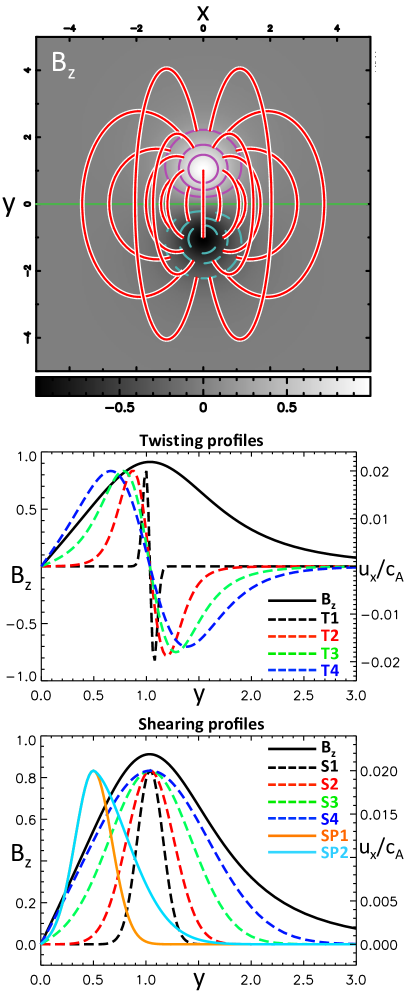
Figure 1.— Top: initial magnetic field configuration of the shearing and twisting simulations. The synthetic magnetogram is represented at the $z=0$ plane with superposed $\pm[0.25;0.50;0.75]$ isocontours of $B_{z}$ (solid purple and dashed cyan) and selected field lines (red). The green line shows the polarity inversion line. Center: photospheric ($z=0$) $B_{z}$ and $u_{x}$ profiles in the $y$ direction for the twisting motions (see Section 2.2). Bottom: same but for the shearing motions (see Section 2.3).

2.2. Photospheric twisting motions

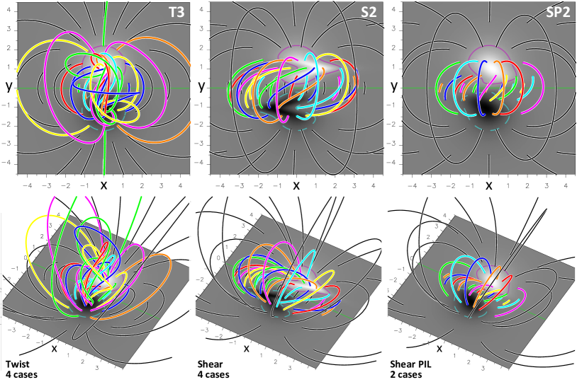
Figure 2.— Top (top row) and 3D (bottom row) views of the magnetic field generated by the photospheric line-tied motions. Left: twist case $\mathrm{T}3$ (Equations (6 – 9)). Center: shear case $\mathrm{S}2$ (Equation (10)). Right: shear case $\mathrm{SP}2$ (Equations (11) and (12)). Current-carrying (potential) magnetic field lines are in color (black).

The first type of photospheric driving is applied to twist the initial potential magnetic configuration along the isocontours of the photospheric vertical magnetic field, $B_{z}(z=0)$. This modifies the transverse components of the initial potential field while preserving its photospheric flux distribution, $B_{z}(z=0,t=0)$. The expression of the twisting velocity field is

$$u_{x}(z=0) = u_{0}\frac{\partial\psi}{\partial y}\,,$$ (6)

$$u_{y}(z=0) = -u_{0}\frac{\partial\psi}{\partial x}\,,$$ (7)

$$u_{z}(z=0) = 0\,,$$ (8)

where $u_{0}$ is a free parameter that controls the maximum speed of the driving, and $\psi$ is a normalized, time-dependent potential (see e.g., Amari et al., 1996; Török & Kliem, 2003; Aulanier et al., 2005). This potential depends on $B_{z}(z=0)$ such that

$$\psi=\frac{B^{2}_{z}(z=0)}{B^{\mathrm{max}\ 2}_{z}(z=0)}\exp\left(\frac{B^{2}_{z}(z=0)-B^{\mathrm{max}\ 2}_{z}(z=0)}{\zeta^{2}_{tw}B^{\mathrm{max}\ 2}_{z}(z=0)}\right)\,,$$ (9)

This twisting profile generates two vortices centered on $\pm B^{\mathrm{max}}_{z}(z=0)$ respectively. The size of the vortices is controlled by the free-parameter $\zeta_{tw}$.

All twisting profiles were applied with a maximum driving speed $u_{0}=0.02c_{A}(t=0)$. LABEL:Fig-BzVel-profiles shows the profiles of $u_{x}(x=0,y)$ for all four cases considered in our study, and referred to as $\mathrm{T}\{1;2;3;4\}$. The corresponding parameters are listed in Table 1. The left panels of LABEL:Fig-B3D display the 3D distribution of the magnetic field for $\mathrm{T}3$.

While the twisting boundary driving analytically preserves the initial distribution of the photospheric vertical magnetic field, small numerical errors eventually deform it on the long run. To ensure that $B_{z}$ is preserved in time for the twisting simulations, we numerically reset $B_{z}(z=0,t)$ to $B_{z}(z=0,t=0)$ at each time step in the course of the runs.

Table 1Values of the parameters for the velocity profiles

Run	$\zeta_{tw}$	$\zeta_{sh}$	$\zeta_{sh1}$	$\zeta_{sh2}$	$y_{0}$	$y_{1}$	$y_{2}$
$\mathrm{T}1$	0.1	-	-	-	1	-	-
$\mathrm{T}2$	0.5	-	-	-	1	-	-
$\mathrm{T}3$	1	-	-	-	1	-	-
$\mathrm{T}4$	5	-	-	-	1	-	-
$\mathrm{S}1$	-	0.17	-	-	1	-	-
$\mathrm{S}2$	-	0.32	-	-	1	-	-
$\mathrm{S}3$	-	0.55	-	-	1	-	-
$\mathrm{S}4$	-	0.77	-	-	1	-	-
$\mathrm{SP}1$	-	-	0.24	0.24	-	0.5	0.5
$\mathrm{SP}2$	-	-	0.24	0.63	-	0.5	0.3

Note. — All values are in non-dimensional units (normalized by half the distance between the two photospheric magnetic polarities).

2.3. Photospheric shearing motions

We consider two types of photospheric shearing motions along the $x$ direction, ${\mathbf{u}}(z=0)=(u_{x},0,0)$. The first is centered on the strongest magnetic field of both photospheric magnetic polarities. The second is confined to the weak field surrounding the PIL to primarily shear it (e.g., similarly to Antiochos et al., 1994).

The first type of shearing motions (curves $\mathrm{S}\{1;2;3;4\}$ in LABEL:Fig-BzVel-profiles) is given by

$$u_{x}(z=0)=u_{0}\ a_{0}\left[\exp\left(-\frac{(y-y_{0})^{2}}{\zeta^{2}_{sh}}\right)-\exp\left(-\frac{(y+y_{0})^{2}}{\zeta^{2}_{sh}}\right)\right]\,.$$ (10)

where $\zeta_{sh}$ controls the width of the shearing, $y_{0}$ corresponds to the $y$-position of the maximum velocity (shearing center), and $a_{0}$ is a constant used for normalization of the Gaussian-profile. The resulting shearing is invariant along the $x$ direction.

The second type of shearing motions (curves $\mathrm{SP}\{1;2\}$ in LABEL:Fig-BzVel-profiles) is given by

$$u_{x}(z=0)=u_{0}\ a_{1}\left[\exp\left(-\frac{(y-y_{1})^{2}}{\zeta^{2}_{sh1}}\right)-\exp\left(-\frac{(y+y_{1})^{2}}{\zeta^{2}_{sh1}}\right)\right]\,,$$ (11)

for $|y|\leq y_{1}$, and

$$u_{x}(z=0)=u_{0}\ a_{2}\left[\exp\left(-\frac{(y-y_{2})^{2}}{\zeta^{2}_{sh2}}\right)-\exp\left(-\frac{(y+y_{2})^{2}}{\zeta^{2}_{sh2}}\right)\right]\,,$$ (12)

for $|y|\geq y_{1}$. Choosing $\zeta_{sh1}\neq\zeta_{sh2}$ allows one to have a broader sheared region either for $|y|<y_{1}$ or $|y|>y_{1}$. The parameter $y_{2}$ is computed to ensure the continuity of the shearing profile at $|y|=y_{1}$, where $u_{x}(|y|=y_{1},z=0)=u_{0}$.

In this paper, we consider four shearing profiles for the first model, referred to as $\mathrm{S}\{1;2;3;4\}$, and two shearing profiles for the second model, referred to as $\mathrm{SP}1$ and $\mathrm{SP}2$. The corresponding parameters are listed in Table 1.

As for the twisting simulations, all shearing profiles were applied with a maximum driving speed $u_{0}=0.02c_{A}(t=0)$ to ensure a quasi-force-free evolution of the magnetic field. The applied profiles are displayed in LABEL:Fig-BzVel-profiles. The middle and left panels of LABEL:Fig-B3D display the 3D distribution of the magnetic field for $\mathrm{S}2$ and $\mathrm{SP}2$, respectively.

2.4. Ramp function

We apply all photospheric line-tied motions using a ramp function to smoothly bring the system from rest to a constant-velocity photospheric driving, such that

$${\mathbf{u}}(x,y,z=0,t)=\gamma(t)\ {\mathbf{u}}(x,y,z=0)\,,$$ (13)

where ${\mathbf{u}}(x,y,z=0)$ is defined in Sections 2.2 and 2.3. The ramp function, $\gamma(t)$, is given by

$$\gamma(t)=\frac{1}{2}\tanh\left(\frac{2(t-t_{m})}{t_{hw}}\right)+\frac{1}{2}\,,$$ (14)

where $t_{m}$ corresponds to the time at which the middle of the ramp function is reached, and $t_{hw}$ corresponds to the half-width of the ramp time. In our runs, we fix $t_{m}=15t_{A}$ and $t_{hw}=5t_{A}$. With these settings, the photospheric driving starts after $\approx 10$ Alfvén times, allowing the system to reach a good numerical equilibrium before the acceleration begins. The constant-velocity photospheric driving is reached after $\approx 20$ Alfvén times.

3. Photospheric currents induced by twisting motions

In cylindrical geometry, any twisting motion based on a twist function that falls to zero at a finite radial distance should generate a twisted flux tube formed of a core of direct currents, fully surrounded by a shell of return currents that exactly neutralize the direct currents (see Appendix A).

The transposition of these results to 3D geometry has often been used to argue that compact photospheric twisting motions should lead to the generation of fully neutralized currents (e.g., Melrose, 1991; Parker, 1996). However, such a transposition disregards the fact that a 3D magnetic flux tube may not systematically have a cylindrical analogue. It is therefore not obvious that the properties of electric currents expected from a simplified, cylindrical geometry may still hold in a more complex 3D one.

To address this issue, we analyze the electric currents generated by compact, photospheric twisting motions (see Section 2.2).

3.1. Photospheric distribution of vertical currents

LABEL:Fig-Jztwist displays the photospheric vertical current density, $j_{z}$, for the twisting runs, a few Alfvén times before each numerical simulation terminated (due to the development of a numerical instability caused by very sharp gradients). Each twisting run induces the generation of a core of negative-direct currents surrounded by a shell of positive-return currents, just as in cylindrical geometry. As reported by Török & Kliem (2003) and Delannée et al. (2008) for similar models, we find that the direct currents are overall stronger and more compact than the return currents. In addition, we notice that the distribution of currents always exhibits the same type of strong azimuthal asymmetry (except for $\mathrm{T}{1}$) that does not occur in cylindrical geometry.

This generic property was already explained by Aulanier et al. (2005) and Titov et al. (2008), and is typical of the 3D loop-geometries analyzed in this paper. This asymmetry is an effect of field-line length resulting from the flux tube curvature. In cylindrical geometry $(r,\theta,z)$, the equations of magnetic field lines and electric current density lead to

$$B_{\theta} = \frac{r\Phi}{l}B_{z}\,,$$ (15)

$$j_{z} = \frac{1}{r}\frac{\partial rB_{\theta}}{\partial r}\propto\frac{B_{\theta}}{r}\propto\frac{\Phi B_{z}}{l}\,,$$ (16)

where $\Phi$ and $l$ are the field-line twist and length, respectively. For a given $B_{z}$ isocontour $\Phi$ is fixed. It then follows that shorter field lines (i.e., smaller $l$) possess a stronger electric current density (Equation (16)). For our 3D curved flux tube, the same amount of twist, $\Phi$, is transferred to each field line of any given isocontour of $B_{z}$. The previous considerations thus imply that stronger currents develop at the footpoints of the shortest field lines of any $B_{z}$ isocontour. This creates an asymmetry that is amplified by the faster expansion of the larger field lines. The advection of this asymmetry by the photospheric motions is responsible for the swirling pattern exhibited by the electric current distribution. This effect is extremely weak for $\mathrm{T}1$ because the twisting vortices are so narrow that the twisted field lines have a very similar length.

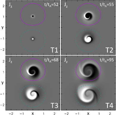
Figure 3.— Photospheric ($z=0$) current maps, $j_{z}$, at the end of each simulations for the symmetric twisting of two opposite magnetic polarities (Section 2.2), for $\mathrm{T}\{1;2;3;4\}$. White and black display positive and negative currents respectively. Values are saturated at $\pm 1.5$. Solid purple and dashed cyan lines represent $\pm 0.25$ isocontours of $B_{z}$.

Among several differences between each simulation, one is the extension of the currents close to the PIL. In particular, for the cases $\mathrm{T}\{1;2\}$, the twisting vortices are so narrow that the distribution of current is mainly localized well inside the isocontour $|B_{z}|=0.25$. On the contrary, for $\mathrm{T}\{3;4\}$, the vortices are so broad that the distribution of current extends to the PIL.

3.2. Evolution of the total direct and return currents

We now analyze the curves of integrated currents by computing

$$I^{\mathrm{X}}_{z}=\int_{y\geq 0}j^{\mathrm{X}}_{z}{\ \mathrm{d}}{\mathcal{S}}\,,$$ (17)

where $X$ refers to the total direct or return current within the positive magnetic polarity (i.e., $y\geq 0$). Because the direct/return currents are negative/positive, we compute the total direct/return current by extracting the negative/positive current density in the positive magnetic polarity.

The temporal evolution of the integrated direct and return currents is presented in the top panel of LABEL:Fig-Iztwist. Due to its small vortex size, the $\mathrm{T}1$ case shows the development of only weak direct and return currents. For the three other cases, the vortices are broader and stronger direct and return currents develop.

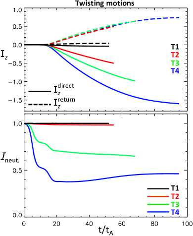
Figure 4.— Evolution of the electric current, $I_{z}$, at $z=0$ in the positive polarity for the photospheric twisting motions. Top: negative-direct ($I^{\mathrm{direct}}_{z}$) and positive-return ($I^{\mathrm{return}}_{z}$) currents (respectively displayed in solid and dashed lines). Bottom: neutralization ratio.

LABEL:Fig-Iztwist shows that the absolute value of the integrated direct current exhibit a monotonic rise (regardless of the vortex width) and the strength of the direct current increases with the width of the twisting vortex. The integrated return current also presents a monotonic behavior. However, the strength of the return current only increases with the vortex width up to $\zeta_{tw}\leq 0.5$.

Increasing the vortex width builds up twist in a larger volume and generates a higher direct current. The return current is affected in a more complex manner, because the boundary between the direct and return currents is pushed closer to the PIL. Away from the PIL, increasing the vortex also implies that longer magnetic field lines are being twisted. As discussed by Aulanier et al. (2005), the resulting fast expansion of these field lines limits their current density.

We therefore conjecture that the increase of total electric current ($|I^{\mathrm{direct}}_{z}|+|I^{\mathrm{return}}_{z}|$) with the vortex size, is caused by a complex competition of three mechanisms: (1) an increase due to the transfer of magnetic twist in a broader region, (2) a saturation/decrease caused by the approach of the line of current reversal to the PIL, and (3) a saturation/decrease induced by the fast expansion of the magnetic field lines.

3.3. Evolution of the neutralization ratio

In order to quantify the neutralization of electric currents generated by photospheric line-tied motions, we define the neutralization ratio, $\mathcal{I}_{\mathrm{neut.}}$, as

$$\mathcal{I}_{\mathrm{neut.}}=\bigg{|}\frac{I^{\mathrm{return}}_{z}}{I^{\mathrm{direct}}_{z}}\bigg{|}\,,$$ (18)

where $I^{\mathrm{direct}}_{z}$ and $I^{\mathrm{return}}_{z}$ are computed from Equation (17). The neutralization ratio is $1$ for fully neutralized currents and 0 for a magnetic field solely containing direct currents.

The bottom panel of LABEL:Fig-Iztwist shows the temporal evolution of the neutralization ratio for the twisting runs. Our goal is to analyze the neutralization of currents for different spatial profiles of photospheric line-tied motions. In the following, we therefore restrict our analysis to the period during which the system evolves in response to a stationary boundary driving, i.e., for $t\gtrsim 20t_{A}$. A brief discussion of the results for the transition phase, $t\in[0;20]t_{A}$, is nonetheless provided in Appendix C.

We find that the electric currents remain fully neutralized ($\mathcal{I}_{\mathrm{neut.}}=1$) during the run with the narrowest vortices ($\mathrm{T}1$), and nearly neutralized ($\mathcal{I}_{\mathrm{neut.}}\approx 0.98$) for the $\mathrm{T}2$ run. On the contrary, the two runs with the larger vortices, $\mathrm{T}\{3;4\}$, exhibit a strong departure from neutralization. This confirms the earlier results of Török & Kliem (2003) that were obtained with different numerical settings.

LABEL:Fig-Iztwist further indicates that the constant boundary driving phase is associated with a slow and weak decrease of the neutralization ratio for run $\mathrm{T}3$. On the contrary, the neutralization ratio of run $\mathrm{T}4$ presents a weak increase followed by a saturation. Such behaviors result from a non-trivial combination of the increase of currents with magnetic twist and the saturation of currents caused by the fast expansion of the largest field lines, as discussed in Section 3.2. Note that for $\mathrm{T}4$, two additional effects are likely involved in the evolution of the neutralization ratio: (1) the twisted flux tube starts to leave the numerical domain (as suggested by the opening of some field lines, not shown here), and (2) the flux tube enters a super-exponential growth phase (cf. the equilibrium curves in Török & Kliem, 2003; Aulanier et al., 2005), leading to a fast expansion of the more twisted field lines compared with the less twisted ones, i.e., for the direct currents. This limits the growth of the direct current more efficiently than that of the return current, which could explain the observed weak increase of the neutralization ratio.

In contrast to cylindrical symmetry (Appendix A), LABEL:Fig-Iztwist shows that twist profiles do not systematically generate neutralized currents in fully 3D twisted flux tubes. Hence, the condition for current neutralization derived in 2.5D geometry cannot be directly transposed to a fully 3D loop geometry such as the one considered in this paper. Indeed, we will show in Section 5 that (1) the condition for current neutralization in 3D is more subtle than in 2.5D, and (2) net currents are associated with 3D coronal fields that do not have any analogue in 2.5D.

4. Photospheric currents induced by shearing motions

In this section, we study the electric currents generated by compact photospheric shearing motions (see Section 2.3).

4.1. Photospheric distribution of vertical currents

LABEL:Fig-Jzshear displays the photospheric vertical current density, $j_{z}$, for the shearing runs. We find that each run presents both negative-direct and positive-return, force-free currents. Their sign are identified from the sign of magnetic helicity transferred to the system. In particular, the chosen shearing motions produce negative magnetic helicity, and hence, negative-direct currents.

For almost all simulations, the direct and return currents have a similar spatial distribution with similar intensities. Two cases, however, do not display the same pattern: $\mathrm{S}3$ and $\mathrm{S}4$ mostly possess direct currents. For these two runs, the return currents are much weaker than the direct ones (e.g., $\approx 7$ times weaker for $\mathrm{S}3$).

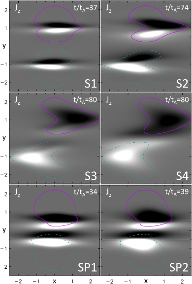
Figure 5.— Photospheric current maps as in LABEL:Fig-Jztwist for the symmetric shearing of two opposite magnetic polarities (Section 2.3). Top/middle: shearing centered on $B^{\mathrm{max}}_{z}$ for $\mathrm{S}\{1;2;3;4\}$. Bottom: shearing centered on the weak field surrounding the PIL for cases $\mathrm{SP}\{1;2\}$. The color coding is the same as in LABEL:Fig-Jztwist with saturation at $\pm 0.5$.

The return currents are, in general, expected for localized shearing motions. This is qualitatively described in LABEL:Fig-Jzshear-Sign with the right-hand rule relating the local magnetic shear with the direction of the electric current. Localized shearing motions generate a curl of the magnetic field that changes sign at the line of strongest magnetic shear. However, contrary to the drawing of Melrose (1991), the line of current reversal may not systematically correspond to that of the maximum velocity. For instance, the maximum photospheric velocity occurs at $|y|=y_{0}=1$ for the $\mathrm{S}\{1;2;3;4\}$ runs. Nevertheless, only $\mathrm{S}\{1;2\}$ possess a current reversal at $|y|\approx y_{0}$ at the photosphere, while it occurs at $|y|\lesssim 0.5$ for $\mathrm{S}3$ and at the PIL for $\mathrm{S}4$. This is because the current distribution depends not only on the shearing velocity profile but also on the 3D shape of magnetic field lines.

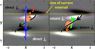
Figure 6.— Examples of sheared magnetic field lines and current direction generated by photospheric shearing motions for the case $\mathrm{S}2$. The thick blue (respectively green) field line is anchored within the direct (respectively return) current. The thick black field line is anchored at the line of current reversal (thin yellow lines). The orange arrows and hands show the direction of current density, ${\mathbf{j}}$, on both sides of the line of current reversal, as inferred from the right-hand rule. The arrows on the field lines indicate the magnetic field direction. The color coding and saturation are the same as in LABEL:Fig-Jzshear.

As for the twisting runs, we find that one significant difference between each shearing simulation is the extension of the currents close to the PIL. In particular, the shearing region of $\mathrm{S}1$ and $\mathrm{S}2$ is so narrow that their distribution of currents is strongly localized (in the $y$-direction) within the isocontour $|B_{z}|=0.25$. On the contrary, the shearing region is so broad for $\mathrm{S}3$ and $\mathrm{S}4$ that the distribution of currents extends to the PIL. Finally, both the shearing profile and electric currents extend to the PIL for $\mathrm{SP}1$ and $\mathrm{SP}2$.

4.2. Evolution of the total direct and return currents

The top panel of LABEL:Fig-Izshear presents the temporal evolution of the integrated direct and return currents in the positive magnetic polarity. All direct current curves show a similar monotonic rise in absolute value with a higher intensity for broader shearing regions. By contrast, the evolution of the return currents varies with the width of the shearing region. For $\mathrm{S}\{1;2\}$, the return current monotonically increases with time. For $\mathrm{S}{3}$, the intensity of the return current increases and then smoothly decreases, while for $\mathrm{SP}\{1;2\}$ the simulation terminated too early to draw conclusions. The $\mathrm{S}4$ run does not show any return current because the line of current reversal occurs at the PIL (cf. Section 4.1).

As shown in Appendix D, the applied shearing motions can generate two evolutionary phases for the current density of magnetic field lines: (1) a first phase of increase with magnetic shear, and (2) a phase of decrease caused by a fast elongation of the field lines. For similar shearing velocities, the shortest field lines should be the first to experience (2), because this effect is more pronounced for field lines that align more rapidly with the PIL (as explained in Appendix D). For all shearing simulations, the return currents are associated with the shortest magnetic field lines. We thus argue that it is the late elongation of these field lines that is responsible for the decrease of return current observed for $\mathrm{S}3$.

Finally, we note that increasing $\zeta_{sh2}$ for the second shearing profile (i.e., $\mathrm{SP}2$), allows one to modify the shear profile of the field lines associated with the direct current. In particular, the direct current is distributed over a broader region. However, the amount of direct and return current is preserved.

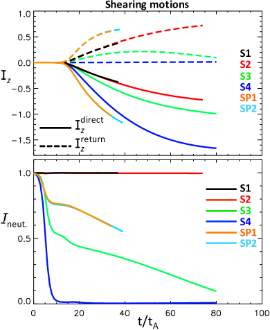
Figure 7.— Evolution of electric current as in LABEL:Fig-Iztwist for the photospheric shearing motions.

4.3. Evolution of the neutralization ratio

The bottom panel of LABEL:Fig-Izshear displays the temporal evolution of the neutralization ratio for each shearing run. For the reasons explained in Section 3.3, we focus our analysis on the neutralization during the constant photospheric driving phase (i.e., $t\gtrsim 20t_{A}$).

The currents remain fully neutralized ($\mathcal{I}_{\mathrm{neut.}}=1$) for $\mathrm{S}1$ and $\mathrm{S}2$. On the contrary, the two runs with the broadest shearing widths ($\mathrm{S}\{3;4\}$) exhibit a strong departure from neutralization. For $\mathrm{S}4$, the neutralization ratio vanishes as a consequence of the absence of return current in the simulation (because the line of current reversal occurs at the PIL; cf. Section 4.1). For $\mathrm{SP}\{1;2\}$, the shearing motions applied close to the PIL also generate a strong net current. Both runs lead to the same degree of current neutralization.

We notice that the curves of neutralization ratio of the $\mathrm{S}3$ and $\mathrm{SP}\{1;2\}$ runs all present a comparable evolution. They all show a continuous decrease. Such a decrease indicates that the rate of current build-up is stronger for the direct current than for the return current. As previously mentioned (Section 4.2), the effect of field line elongation more strongly affects the shortest field lines. One then expects a lower rate of current build-up for the return current than for the direct one. This could then explain the continuous decrease of neutralization ratio observed for the $\mathrm{SP}\{1;2\}$ and $\mathrm{S}3$ runs.

Finally, the decreasing behavior of the neutralization ratio of $\mathrm{S}3$ and $\mathrm{SP}\{1;2\}$ indicates that, in a system driven by stationary shearing motions, the neutralization state of the system is not solely determined by the spatial properties of the shearing motions, but also depends on the amount of accumulated shear and inflation.

5. Discussion

In this section, we first examine the development of weak compression currents in the ambient field of our simulations. We then discuss our results in the framework of the sheared-PIL/net current relationship and confront them to the conjectures of Melrose (1991) and Parker (1996).

5.1. Compression currents in the ambient field

When analyzing the distribution of currents of our 3D current-carrying fields at high saturation levels, we find that some very weak currents develop in the ambient field rooted in areas where the photospheric flows vanish (as pointed by the red arrows in LABEL:Fig-3D-compression-currents). These currents are typically $2-3$ orders of magnitude smaller than the currents directly generated by the photospheric flows. They appear in the very close vicinity of the twisted/sheared fields and very rapidly decrease away from them. We find that these currents are induced by the local compression of the ambient field caused by the inflation of the twisted/sheared field in response to the photospheric flows. Such a compression of the ambient field cannot be reproduced in 2.5D geometry because the imposed symmetry forces that field to stay potential.

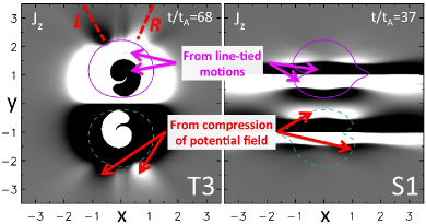
Figure 8.— Saturated photospheric $j_{z}$ (gray shading) showing the currents associated with the compression of the ambient field caused by the inflation of the twisted (left) and sheared (right) magnetic fields. The saturation value is $2.4\times 10^{-3}$ for $\mathrm{T}3$ and $5\times 10^{-3}$ for $\mathrm{S}1$ (compared with Figures 3 and 5 where the saturation value is two orders of magnitude higher). The solid-purple and cyan-dashed lines are $|B_{z}|=0.25$-isocontours.

We also note that the compression currents do not form a shell of a single sign around the return current for the twisting cases (cf. $\mathrm{T}3$ in LABEL:Fig-3D-compression-currents). On the contrary, we find two regions of enhanced currents oriented in two specific directions (as indicated by the dashed red lines in LABEL:Fig-3D-compression-currents). This is caused by the development of a kink of the flux tube axis. The direction of the $L$-dashed red line corresponds to the orientation of the kink of the flux tube axis (as shown in LABEL:Fig-B3D top left and more precisely by the yellow field line in Figure 5 of Aulanier et al., 2005). The kink of the axis causes a preferential compression of the ambient field in its direction, and induces a magnetic depression in the direction of the $R$-dashed red line.

5.2. The sheared-PIL/net current relationship

The numerical experiments of Sections 3 and 4 show that photospheric line-tied motions can generate 3D force-free magnetic fields with different amount of current neutralization. We further analyzed and compared the simulations presented in this paper to identify the origin of these various degrees of neutralization. The results are summarized in LABEL:Fig-Neutralized-vs-Net-Currents that displays the photospheric transverse magnetic field at the PIL for current-neutralized and net current cases. We find that all current-neutralized magnetic fields possess a PIL fully embedded in a potential magnetic field (LABEL:Fig-Neutralized-vs-Net-Currents left column). On the contrary, we observe that (1) a net current develops simultaneously with magnetic shear at the PIL, and (2) a stronger net current is induced for simulations generating a stronger magnetic shear at the PIL (see LABEL:Fig-Neutralized-vs-Net-Currents right column). In agreement with Török & Kliem (2003), and extending their results to pure shearing motions, we thus find that a net current solely develops when magnetic shear is built up at the PIL. These results are also consistent with observational studies (e.g., Ravindra et al., 2011; Georgoulis et al., 2012) and the investigation of flux emergence in Török et al. (2014). In the following, we address this relationship in a general form.

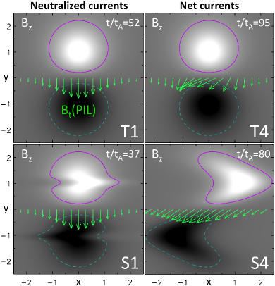
Figure 9.— Sheared-PIL/net current relationship illustrated for two current-neutralized ($\mathrm{T}1$ and $\mathrm{S}1$; left column) and two net current ($\mathrm{T}4$ and $\mathrm{S}4$; right column) simulations. The photospheric transverse magnetic field at the PIL, ${\mathbf{B}}_{t}(\mathrm{PIL})$ (green arrows), is plotted over the photospheric $B_{z}$ (gray shading). The solid-purple and cyan-dashed lines are $|B_{z}|=0.25$-isocontours.

We consider a bipolar potential magnetic field such as the initial field used in our numerical simulations (LABEL:Fig-ShearedPIL-NetI). We then consider a photospheric velocity field, ${\mathbf{u}}$, that builds up electric currents at $z=0$ inside of a surface, $S_{u}$, of the positive magnetic polarity; ${\mathbf{u}}$ vanishes outside of $S_{u}$. Finally, we consider a closed curve, $\mathcal{C}$, such that (i) $\mathcal{C}$ includes the PIL of the bipolar AR, and (ii) the surface, $S$, enclosed by $\mathcal{C}$ is much larger than the surface $S_{u}$ where electric currents are generated by the photospheric motions. These two choices ensure that all the currents transferred to the magnetic field are fully enclosed by $\mathcal{C}$.

The applied photospheric velocity field generates a current-carrying component, ${\mathbf{B}}_{j}$, in the bipolar magnetic field. The total magnetic field, ${\mathbf{B}}$, can be decomposed as the sum of its potential, ${\mathbf{B}}_{p}$, and current-carrying, ${\mathbf{B}}_{j}$, components (e.g., Valori et al., 2013), such that

$${\mathbf{B}} = {\mathbf{B}}_{p}+{\mathbf{B}}_{j}\,,$$ (19)

$${\bf\nabla}\times{\mathbf{B}} = {\bf\nabla}\times{\mathbf{B}}_{j}=\mu_{0}{\mathbf{j}}\,.$$ (20)

In fact, ${\mathbf{B}}_{j}$ can be further decomposed into two components

$${\mathbf{B}}_{j}={\mathbf{B}}^{{\mathbf{u}}\neq 0}_{j}+{\mathbf{B}}^{{\mathbf{u}}=0}_{j}\,.$$ (21)

${\mathbf{B}}^{{\mathbf{u}}\neq 0}_{j}$ corresponds to the main current-carrying field and it has non-zero values only in the magnetic field connected to $S_{u}$. ${\mathbf{B}}^{{\mathbf{u}}=0}_{j}$ is a current-carrying field generated by the compression of the potential field resulting from the inflation of the main current-carrying field. This component is non-zero only in the ambient magnetic field, i.e., the magnetic field not connected to $S_{u}$. Its strength is on average two orders of magnitude smaller than the strength of the main current-carrying field, ${\mathbf{B}}^{{\mathbf{u}}\neq 0}_{j}$, and decreases very rapidly away from the latter (cf. Section 5.1). For this reason and because the contour $\mathcal{C}$ is chosen such that $S$ is much larger than $S_{u}$, we can neglect ${\mathbf{B}}^{{\mathbf{u}}=0}_{j}$ in the following.

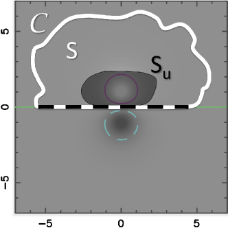
Figure 10.— Schematic used for the mathematical demonstration of the sheared-PIL/net current relationship. The map shows a photospheric magnetogram of the initial potential magnetic field used in our line-tied simulations. The surfaces $S/S_{u}$ and the contour $\mathcal{C}$ are defined in Section 5.2. The thick, black/white, dashed line highlights the part of $\mathcal{C}$ that corresponds to the PIL (green solid line). The solid purple, and dashed cyan, lines are $B_{z}=\pm 0.25$-isocontours of the magnetic field.

Applying Ampère’s law, it then follows that the total electric current enclosed by $\mathcal{C}$ is

$$I = \frac{1}{\mu_{0}}\oint_{\mathcal{C}}{\mathbf{B}}_{j}\cdot~{}{\mathrm{d}}\mathbf{l}\,$$ (22)

$$\approx \frac{1}{\mu_{0}}\oint_{\mathcal{C}}{\mathbf{B}}^{{\mathbf{u}}\neq 0}_{j}\cdot~{}{\mathrm{d}}\mathbf{l}\,,$$

where $~{}{\mathrm{d}}\mathbf{l}$ is the line element along $\mathcal{C}$. Equation (22) can be further decomposed as the sum of two contributions: one along the part of $\mathcal{C}$ corresponding to the PIL, and a second corresponding to the remaining of $\mathcal{C}$ (i.e., $\mathcal{C}-PIL$). This leads

$$I\approx\frac{1}{\mu_{0}}\left(\int_{PIL}{\mathbf{B}}^{{\mathbf{u}}\neq 0}_{j}\cdot~{}{\mathrm{d}}\mathbf{l}\ +\ \int_{\mathcal{C}-PIL}{\mathbf{B}}^{{\mathbf{u}}\neq 0}_{j}\cdot~{}{\mathrm{d}}\mathbf{l}\right)\,.$$ (23)

The intersection of $\mathcal{C}$ with $S_{u}$ — when it exists — is limited to the PIL, and ${\mathbf{B}}^{{\mathbf{u}}\neq 0}_{j}$ vanishes outside $S_{u}$. It then follows that the second term of Equation (23) vanishes. At any fixed time, the total current enclosed by $\mathcal{C}$ is therefore

$$I\approx\frac{1}{\mu_{0}}\int_{PIL}{\mathbf{B}}^{{\mathbf{u}}\neq 0}_{j}\cdot\mathbf{dl}\,.$$ (24)

When the PIL is embedded within a potential magnetic field, i.e., $S_{u}$ is never in contact with the PIL, then ${\mathbf{B}}^{{\mathbf{u}}\neq 0}_{j}$ vanishes all along the PIL. The total electric current, $I$, thus vanishes as well, which implies that the currents are neutralized. On the contrary, ${\mathbf{B}}^{{\mathbf{u}}\neq 0}_{j}$ does not vanish for a magnetically-sheared PIL. The current-carrying magnetic field will then contain a net electric current, $I\neq 0$ (unless the integrand in Equation (24) changes sign such that the oppositely directed contributions cancel exactly, which could happen for the very rare cases of ARs containing opposite twist/shear). We thus conclude that force-free net currents are inevitably related to magnetically sheared PILs.

The above derivation is supported by the results of the $\mathrm{SP2}$ run as compared with $\mathrm{SP}1$. Indeed, both possess the same shearing profile in the field lines associated with the return current. This means that both simulations have approximately the same magnetic shear profile along the PIL (neglecting the effect of different distant direct currents). From Equation (24), it follows that both are expected to have very similar net current. This is what happens as inferred in LABEL:Fig-Izshear from the curves of direct current, return current, and neutralization ratio of $\mathrm{SP}2$ which match those of $\mathrm{SP}1$.

Finally, we emphasize that the above relationship between net currents and magnetically sheared PIL is significantly different from the Lorentz-force-driven shear discussed by Georgoulis et al. (2012). Indeed, in all our zero-$\beta$ MHD simulations, there is no dynamical compression that could generate a Lorentz force which would shear the PIL. On the contrary, the magnetic shear along the PIL is caused by the motions imposed in the photosphere, and this magnetic shear generates a force-free net current.

5.3. Net currents versus neutralization predictions

The possibility of generating coronal magnetic fields carrying a net current is at variance with the conjectures of Melrose (1991) and Parker (1996) who argued that twisted and sheared coronal fields should be perfectly current-neutralized. The main difference with our results relies in the fact that both authors built a conjecture using 2.5D considerations which were then directly transposed to 3D geometry. The cornerstone of their conjectures is that any 3D twisted/sheared magnetic field embedded in a potential field or field-free environment can be equivalently described by a flux tube connecting two parallel planes and set in the same (but 2.5D) magnetic environment.

The above assumption is valid for any 3D flux tube whose two photospheric magnetic polarities are fully separated either by an ambient potential field or a field-free environment, i.e., when there is no magnetic shear at the PIL. This is the implicit assumption of Melrose (1991) who limited his considerations to the case of twisting and shearing motions not extending to the PIL. The same assumption is also implicitly made by Parker (1996) when using a cylindrical twisted flux tube of finite radius as a model for an element of an AR magnetic field which is fragmented in the photosphere. In such cases, a 2.5D analysis shows that electric currents should be neutralized (see Appendix A). This agrees with our 3D derivation of Section 5.2 in which we demonstrated that full current neutralization occurs when a PIL is fully embedded in a potential field or field-free environment.

On the contrary, when a 3D flux tube has magnetic shear along its PIL, the above cylindrical description of an AR is not valid. Indeed, an electric current is then flowing along the PIL where the two polarities are in contact. Then, the cylindrical approximation of Melrose (1991) and Parker (1996) is not relevant. As a consequence, the associated conclusion that currents should be neutralized is not applicable. A fully 3D analysis is then required to predict whether or not currents should be neutralized. Such a 3D analysis actually show that a net current should be expected when magnetic shear is present along the PIL of the 3D flux tube (cf. Section 5.2).

6. Conclusions

In this study, we used 3D MHD numerical simulations to analyze the properties of electric currents in line-tied coronal fields generated by photospheric flows in bipolar ARs. We showed that typical photospheric flows, such as twisting and shearing motions, invariably produce both direct and return currents in the line-tied coronal fields. We find that these photospheric flows can create both neutralized and non-neutralized currents.

Using Ampère’s law, we provided a physical origin to the build-up of force-free net currents in coronal magnetic fields. They arise from the development of magnetic shear along PILs (Section 5.2). This conclusion agrees with the independent study of Török et al. (2014) who showed that magnetic flux emergence can also produce a net coronal current which simultaneously develops with magnetic shear at the PIL. Török et al. (2014) and our study thus set a theoretical framework for understanding the properties of electric currents in ARs. They both show that, in general, net currents can be formed in the corona from various, independent and/or combined processes: e.g., magnetic flux emergence, photospheric flows, and by extension, any mechanism that can generate magnetic shear along a PIL.

Net currents in ARs can therefore develop in a large variety of cases. On the contrary, the production of perfectly current-neutralized magnetic fields in the solar atmosphere is a special case that requires a rather uncommon condition: a main PIL without magnetic shear. This is unlikely for both emerging and evolved/decaying ARs. Indeed, several observational and numerical studies show that newly emerged ARs generally possess a strongly sheared PIL (e.g., Manchester et al., 2004; Canou et al., 2009; Georgoulis et al., 2012; Toriumi et al., 2013; Poisson et al., 2015). Next, evolved/decaying ARs are often associated with the presence of H$\alpha$ filaments, which are cold dense material supported in highly sheared/twisted magnetic fields lying above PILs (e.g., van Ballegooijen & Martens, 1989; Aulanier & Demoulin, 1998; Gibson et al., 2004; Schmieder et al., 2006; Jing et al., 2010; Mackay et al., 2010; Xia et al., 2014).

Furthermore, starting from a configuration with an un-sheared PIL, it will remain so if the shear component of photospheric flows is not extending to the PIL. This is also unlikely since the opposite is typically observed in ARs (e.g., Vemareddy et al., 2012; Wang et al., 2012; Guo et al., 2013; Liu et al., 2013). In fact, several observations suggest shearing profiles that would be analogous to our strongly non-neutralized run $\mathrm{S}4$ (as inferred from the photospheric motions of magnetic polarities; e.g., Su et al., 2007; Sun et al., 2012). Finally, the absence of significant shear is more likely to hold for evolved ARs possessing isolated magnetic polarities (i.e., magnetic polarities far away from each other).

The two main sources of AR currents, emergence and horizontal photospheric motions, would thus be expected to primarily produce net coronal currents. Nevertheless, a few observational studies seem to indicate that ARs with neutralized currents may be as numerous as ARs with a net current (e.g., Wilkinson et al., 1992; Wheatland, 2000). If we consider a typical magnetic field of $B_{\mathrm{max}}=2000\ \mathrm{G}$ for newly emerged ARs, and $15\ \mathrm{Mm}$ for one spatial unit of our non-dimensionalized simulations, the strength of the net current in our strongly non-neutralized magnetic fields can reach $\sim 0.7-4\ \times 10^{12}\ \mathrm{A}$. If the magnetic field is scaled to $B_{\mathrm{max}}=200\ \mathrm{G}$ for decaying ARs, the strength of the net current ranges between $\sim 0.7-4\ \times 10^{11}\ \mathrm{A}$. Since the actual measurement precision is about $10^{11}\ \mathrm{A}$, it then remains to be proved that current-neutralized ARs are truly current-neutralized. This requires a systematic analysis of both the current-neutralization and the magnetic shear at the PIL for any studied AR, which was not done in Wilkinson et al. (1992) and Wheatland (2000). Such dedicated studies could then be used to further test the conclusions derived in the present paper.

Finally, even though our MHD simulations systematically report the presence of return currents, net currents in coronal magnetic fields do exist. Therefore, eruption models based on magnetic configurations possessing net currents (e.g., van Tend & Kuperus, 1978; Heyvaerts et al., 1982; Lin et al., 1998; Titov & Démoulin, 1999; Kliem & Török, 2006; Démoulin & Aulanier, 2010) are a simplified, but valid, description of pre-eruptive magnetic fields in ARs. Our results that relate net coronal currents to magnetically-sheared PILs then naturally explain the observational conclusions of Falconer (2001) and Falconer et al. (2002), which state that ARs with a sheared PIL are more CME-prolific. That being said, one must bear in mind that the aforementioned analytical models, based on a net coronal current, do not possess any return current. Yet, return currents exist in MHD simulations of CMEs (e.g., Török & Kliem, 2003; Delannée et al., 2008; Aulanier et al., 2012). Moreover, in some cases the return current can have the same strength as the direct current, which may inhibit the eruption (e.g., Forbes, 2010). Further studies are then required to quantify the role of these return currents for the trigger and development of solar flares and CMEs, e.g., using MHD simulations.

Appendix A A. Electric currents in cylindrical geometry

Let us consider a twisted magnetic flux tube in cylindrical geometry. The cylindrical coordinates $r$, $\theta$, and $z$, respectively describe the distance to the axis of the flux tube, the angle around its axis, and the position along its axis. Using the integrated form of Ampère’s law, the total current, $I$, flowing across a disk of radius $r$, is

$$\mu_{0}\ f\ I(r)=2\pi\ r\ B_{\theta}(r)\,,$$ (A1)

where $f$ (equals $+1$ or $-1$) is included so that $I(r)$ is a positive function in the flux rope core where the direct current is located. In the flux rope core, the current $I$ is therefore a growing function of $r$. The region of return current is located where $I$ is a decreasing function of $r$, so for

$$\frac{\partial\left(rB_{\theta}\right)}{\partial r}<0\,.$$ (A2)

The existence of return currents is thus simply constrained by the existence of $r_{l}>0$, such that

$$B_{\theta}(r)<\frac{C}{r}\,,\ \mathrm{for}\ r>r_{l}\,,$$ (A3)

where $C$ is an integration constant. The region where $B_{\theta}$ decreases faster than $1/r$ is the region of return current.

The flux rope current is fully neutralized if there is a finite radius, $r_{c}$, such that $I(r>r_{c})=0$, i.e.,

$$B_{\theta}(r)=0\,,\ \mathrm{for}\ r>r_{c}\,.$$ (A4)

From Equation (A1), it is straightforward to show that if a twisted magnetic flux tube is confined (i.e., if it has a finite radius $R=r_{c}$), then the total electric current carried by the flux tube vanishes.

These conditions are valid regardless of the force-freeness of the magnetic field.

Appendix B B. Solenoidal conditions with OHM

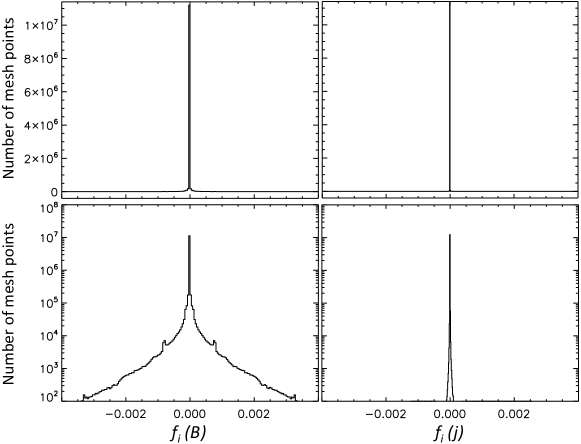
Figure 11.— PDF of the fractional flux, $f_{i}$ (Equation (B2)), of the magnetic field (left) and of the electric current density (right), for the twisting simulation $\mathrm{T}4$ at $t=60\ t_{A}$. Top: linear scale. Bottom: log-scale.

As mentioned in Section 2.1, the solenoidal condition for the magnetic field is not numerically imposed in the code. However, to show that it does not affect the evolution of the magnetic field in our simulations, we compute the fraction of non-conserved flux, or fractional flux, $f_{i}$, within each cell, $i$, of the mesh, such that

$$f_{i}({\mathbf{X}}) = \frac{\int_{v_{i}}\nabla\cdot{\mathbf{X}}_{i}{\ \mathrm{d}}v_{i}}{\int_{s_{i}}|{\mathbf{X}}_{i}|{\ \mathrm{d}}s_{i}}\,$$ (B1)

$$\approx \frac{v_{i}}{s_{i}}\frac{\nabla\cdot{\mathbf{X}}_{i}}{|{\mathbf{X}}_{i}|}\,,$$ (B2)

where $|{\mathbf{X}}_{i}|$ and $\nabla\cdot{\mathbf{X}}_{i}$ are respectively the norm of ${\mathbf{X}}$, and its divergence, within the mesh-cell, $i$, of volume, $v_{i}$, bounded by the surface, $s_{i}$ (e.g., Wheatland et al. 2000; Valori et al. 2013).

We compute the set of $f_{i}({\mathbf{B}})$ values for the twisted flux tube simulation, $\mathrm{T}4$. The corresponding probability density function (PDF) and its statistics are displayed in LABEL:Fig-PDF-Solenoidal-Conditions and Table 2. As one can see, the PDF is well centered on zero. The two bumps in the wings of the PDF are contributions from the boundaries.

Table 2Statistics of the pdf of fractional flux, $f_{i}$.

${\mathbf{X}}$	$<f_{i}({\mathbf{X}})>$	median of $|f_{i}({\mathbf{X}})|$	$<|f_{i}({\mathbf{X}})|>$	$\sigma(f_{i}({\mathbf{X}}))$	$\sqrt{<f({\mathbf{X}})^{2}_{i}>}$
${\mathbf{B}}$	$-1\times 10^{-10}$	$2.3\times 10^{-7}$	$2.8\times 10^{-5}$	$1.7\times 10^{-4}$	$1.7\times 10^{-4}$
${\mathbf{j}}$	$2.1\times 10^{-11}$	$3.3\times 10^{-8}$	$2.9\times 10^{-7}$	$2.5\times 10^{-6}$	$2.5\times 10^{-6}$

Note. — ${\mathbf{B}}$ and ${\mathbf{j}}$ respectively are the magnetic field and the electric current density. $<>$ and $\sigma$ respectively are the mean and standard deviation. Results are presented for the simulation $\mathrm{T}4$ at $t=60\ t_{A}$.

Both LABEL:Fig-PDF-Solenoidal-Conditions and Table 2 show a mean, a median, and a standard deviation of $f_{i}$, that are all smaller than $\sim 10^{-4}$. This means that the amount of non-conserved magnetic flux within each mesh-cell is typically $\sim 10^{4}$ times weaker than the local magnetic flux. Therefore, even though the solenoidal condition is not numerically treated within the OHM code, the non-conservation of magnetic flux remains very weak. These results are representative of the set of numerical simulations performed and presented in this paper. We thus conclude that the solenoidal condition is well enough verified to ensure that the very weak non-conservation of magnetic flux does not affect the evolution of the system in each of our line-tied simulations.

We further compute the fractional flux for the electric current density ($f_{i}({\mathbf{j}})$) to check that its divergence is indeed zero (as one would expect from applying the divergence operator to Ampère’s law). The associated PDF, and the statistics of the PDF, are displayed in LABEL:Fig-PDF-Solenoidal-Conditions and Table 2. As for the magnetic field, $\nabla\cdot{\mathbf{j}}=0$ is well preserved in our line-tied simulations.

Appendix C C. Neutralization ratio: transition phase

The neutralization ratio curves of the partially current-neutralized cases all present a transition phase between $t=0$ and $t\approx 20t_{A}$. This transition phase is distinguished by two specific periods, $t=[0;10]t_{A}$ and $t=[10;20]t_{A}$.

As mentioned Section 3.2, the direct/return currents are computed by extracting the negative/positive current density at the photospheric positive polarity. During the early evolution of the system (when the driving is zero and/or extremely weak), the computed total direct/return current, and hence neutralization ratio, are all dominated by the noise. This noise is essentially due to the presence of magneto-acoustic waves at early times. While the initial potential field is analytically potential and at equilibrium, it is not numerically because of the discretization. This well-known effect leads to the generation of magneto-acoustic waves inducing compression of the magnetic field. Such a compression creates transitory neutralized currents in each magnetic polarity of the system because they are not associated with magnetic shear build-up at the PIL. This is why the neutralization ratio is initially well-defined and equal to 1 for all simulations. A precise analysis shows us that the currents generated by the photospheric motions progressively become dominant (i.e., their strength is $\sim 100$ times larger than the noise) for $t\gtrsim 10t_{A}$. The transition from a system dominated by noise currents towards photospherically-generated currents is thus responsible for the early evolution of the neutralization ratio, up to $10t_{A}$.

The second transition appears between $t=[10;20]t_{A}$, which corresponds to the main acceleration period of the temporal ramp function. This transition follows the evolution of the temporal ramp function. Such a transition could be produced by two competitive mechanisms: (1) non-force-free effects due to the fast acceleration of the photospheric velocities, and (2) the saturation of currents due to field line length (as discussed in Sections 3.2 and 4.2).

Appendix D D. Return current decrease in shearing runs

Let us consider a magnetic field line at a time $t$. We define $\rho$ as the distance between its two photospheric footpoints. $x_{0}$ and $y_{0}$ are the distance between both photospheric footpoints in the $x$ and $y$ direction respectively, such that

$$x_{0} = \rho\sin\phi\,$$ (D1)

$$y_{0} = \rho\cos\phi\,,$$ (D2)

where $\phi$ is the angle between the field line footpoints and the normal to the PIL at the photosphere. The variation of these distances during an infinitesimal time, $\mathrm{d}t$, is

$$\mathrm{d}x_{0} = \mathrm{d}\rho\sin\phi+\rho\cos\phi\ \mathrm{d}\phi\,$$ (D3)

$$\mathrm{d}y_{0} = \mathrm{d}\rho\cos\phi-\rho\sin\phi\ \mathrm{d}\phi\,.$$ (D4)

The photospheric motions being solely applied in the $x$ direction, it follows that $\mathrm{d}y_{0}=0$. Combining with Equations (D3) and (D4), one obtains the following equations

$$\mathrm{d}\rho = \sin\phi\ \mathrm{d}x_{0}\,$$ (D5)

$$\rho\mathrm{d}\phi = \cos\phi\ \mathrm{d}x_{0}\,.$$ (D6)

Then, we define $|\epsilon|=|\phi-\phi_{0}|\ll 1$. Replacing in Equations (D5) and (D6) and expanding terms to a first order in $\epsilon$, one obtains

$$\mathrm{d}\rho \approx \left(\sin\phi_{0}+\epsilon\cos\phi_{0}\right)\ \mathrm{d}x_{0}\,$$ (D7)

$$\rho\mathrm{d}\phi \approx \left(\cos\phi_{0}-\epsilon\sin\phi_{0}\right)\ \mathrm{d}x_{0}\,.$$ (D8)

When the footpoints segment is close to the normal to the PIL, $\phi_{0}=0$. It follows that $\mathrm{d}\rho\approx\epsilon\mathrm{d}x_{0}\ll\rho\mathrm{d}\phi\approx\mathrm{d}x_{0}$. The boundary driving essentially induces a rotation of the field line with regard to the vertical direction. In other words, it shears the magnetic field line, thus increasing its current density. On the contrary, when the footpoints segment is almost aligned with the PIL, $\phi_{0}=\pi/2$. Then, $\mathrm{d}\rho\approx\mathrm{d}x_{0}\gg\rho\mathrm{d}\phi\approx-\epsilon\mathrm{d}x_{0}$. The boundary driving essentially increases the distance between the field line footpoints. Since this distance is related to the field line length (larger footpoints distance implies larger field line), it follows that the photospheric motions essentially increase the length of the field line, hence reducing its current density (cf. Equation (16); see also Aulanier et al. 2005).

We then conclude that the continuous shearing of each magnetic field line can generate two evolutionary phases for their current density: (1) a first phase of increase with magnetic shear, and (2) a phase of decrease due to a fast elongation of the field lines. The shortest magnetic field lines (i.e., with the smallest $y_{0}$) should be the first to be affected by the decrease of current due to their elongation because they align more rapidly with the PIL. For a given $x_{0}$, smaller values of $y_{0}$ induce larger values of $\tan\phi(t)=x_{0}/y_{0}$, and hence, values of $\phi(t)$ closer to $\pi/2$ (i.e., the value for which the field line is aligned with the PIL).

References

- Amari et al. (1996) Amari, T., Luciani, J. F., Aly, J. J., & Tagger, M. 1996, ApJ, 466, L39
- Antiochos et al. (1994) Antiochos, S. K., Dahlburg, R. B., & Klimchuk, J. A. 1994, ApJ, 420, L41
- Aulanier (2014) Aulanier, G. 2014, in IAU Symposium, Vol. 300, IAU Symposium, ed. B. Schmieder, J.-M. Malherbe, & S. T. Wu, 184–196
- Aulanier & Demoulin (1998) Aulanier, G. & Demoulin, P. 1998, A&A, 329, 1125
- Aulanier et al. (2005) Aulanier, G., Démoulin, P., & Grappin, R. 2005, A&A, 430, 1067
- Aulanier et al. (2012) Aulanier, G., Janvier, M., & Schmieder, B. 2012, A&A, 543, A110
- Aulanier et al. (2010) Aulanier, G., Török, T., Démoulin, P., & DeLuca, E. E. 2010, ApJ, 708, 314
- Canou et al. (2009) Canou, A., Amari, T., Bommier, V., et al. 2009, ApJ, 693, L27
- Chandra et al. (2010) Chandra, R., Pariat, E., Schmieder, B., Mandrini, C. H., & Uddin, W. 2010, Sol. Phys., 261, 127
- Cheung & Isobe (2014) Cheung, M. C. M. & Isobe, H. 2014, Living Reviews in Solar Physics, 11, 3
- Dalmasse et al. (2015) Dalmasse, K., Chandra, R., Schmieder, B., & Aulanier, G. 2015, A&A, 574, A37
- Delannée et al. (2008) Delannée, C., Török, T., Aulanier, G., & Hochedez, J.-F. 2008, Sol. Phys., 247, 123
- Démoulin & Aulanier (2010) Démoulin, P. & Aulanier, G. 2010, ApJ, 718, 1388
- Falconer (2001) Falconer, D. A. 2001, J. Geophys. Res., 106, 25185
- Falconer et al. (2002) Falconer, D. A., Moore, R. L., & Gary, G. A. 2002, ApJ, 569, 1016
- Falconer et al. (2006) Falconer, D. A., Moore, R. L., & Gary, G. A. 2006, ApJ, 644, 1258
- Fan (2009) Fan, Y. 2009, Living Reviews in Solar Physics, 6, 4
- Forbes (2010) Forbes, T. 2010, Models of coronal mass ejections and flares (Cambridge University Press), 159
- Georgoulis et al. (2012) Georgoulis, M. K., Titov, V. S., & Mikić, Z. 2012, ApJ, 761, 61
- Gibson et al. (2004) Gibson, S. E., Fan, Y., Mandrini, C., Fisher, G., & Demoulin, P. 2004, ApJ, 617, 600
- Gosain et al. (2014) Gosain, S., Démoulin, P., & López Fuentes, M. 2014, ApJ, 793, 15
- Guo et al. (2013) Guo, Y., Ding, M. D., Cheng, X., Zhao, J., & Pariat, E. 2013, ApJ, 779, 157
- Heyvaerts et al. (1982) Heyvaerts, J., Lasry, J. M., Schatzmann, M., & Witomsky, P. 1982, A&A, 111, 104
- Janvier et al. (2013) Janvier, M., Aulanier, G., Pariat, E., & Démoulin, P. 2013, A&A, 555, A77
- Jing et al. (2010) Jing, J., Yuan, Y., Wiegelmann, T., et al. 2010, ApJ, 719, L56
- Kliem & Török (2006) Kliem, B. & Török, T. 2006, Physical Review Letters, 96, 255002
- Klimchuk & Sturrock (1992) Klimchuk, J. A. & Sturrock, P. A. 1992, ApJ, 385, 344
- Leake et al. (2013) Leake, J. E., Linton, M. G., & Török, T. 2013, ApJ, 778, 99
- Leka et al. (1996) Leka, K. D., Canfield, R. C., McClymont, A. N., & van Driel-Gesztelyi, L. 1996, ApJ, 462, 547
- Leka & Skumanich (1999) Leka, K. D. & Skumanich, A. 1999, Sol. Phys., 188, 3
- Lin et al. (1998) Lin, J., Forbes, T. G., Isenberg, P. A., & Démoulin, P. 1998, ApJ, 504, 1006
- Liu et al. (2013) Liu, Y., Zhao, J., & Schuck, P. W. 2013, Sol. Phys., 287, 279
- Longcope & Welsch (2000) Longcope, D. W. & Welsch, B. T. 2000, ApJ, 545, 1089
- Low (1977) Low, B. C. 1977, ApJ, 212, 234
- Mackay et al. (2010) Mackay, D. H., Karpen, J. T., Ballester, J. L., Schmieder, B., & Aulanier, G. 2010, Space Sci. Rev., 151, 333
- Manchester et al. (2004) Manchester, IV, W., Gombosi, T., DeZeeuw, D., & Fan, Y. 2004, ApJ, 610, 588
- Martens (1987) Martens, P. C. H. 1987, Sol. Phys., 107, 95
- McClymont & Fisher (1989) McClymont, A. N. & Fisher, G. H. 1989, Washington DC American Geophysical Union Geophysical Monograph Series, 54, 219
- Melrose (1991) Melrose, D. B. 1991, ApJ, 381, 306
- Melrose (1995) Melrose, D. B. 1995, ApJ, 451, 391
- Metcalf et al. (2006) Metcalf, T. R., Leka, K. D., Barnes, G., et al. 2006, Sol. Phys., 237, 267
- Moreno-Insertis (1997) Moreno-Insertis, F. 1997, Mem. Soc. Astron. Italiana, 68, 429
- Parker (1955) Parker, E. N. 1955, ApJ, 121, 491
- Parker (1996) Parker, E. N. 1996, ApJ, 471, 485
- Poisson et al. (2015) Poisson, M., Mandrini, C. H., Démoulin, P., & López Fuentes, M. 2015, Sol. Phys., 290, 727
- Ravindra et al. (2011) Ravindra, B., Venkatakrishnan, P., Tiwari, S. K., & Bhattacharyya, R. 2011, ApJ, 740, 19
- Rust et al. (1994) Rust, D. M., Sakurai, T., Gaizauskas, V., et al. 1994, Sol. Phys., 153, 1
- Schmieder et al. (2006) Schmieder, B., Aulanier, G., Mein, P., & López Ariste, A. 2006, Sol. Phys., 238, 245
- Schmieder et al. (2004) Schmieder, B., Mein, N., Deng, Y., et al. 2004, Sol. Phys., 223, 119
- Schrijver et al. (2005) Schrijver, C. J., De Rosa, M. L., Title, A. M., & Metcalf, T. R. 2005, ApJ, 628, 501
- Shibata & Magara (2011) Shibata, K. & Magara, T. 2011, Living Reviews in Solar Physics, 8, 6
- Su et al. (2007) Su, Y., Golub, L., van Ballegooijen, A., et al. 2007, PASJ, 59, 785
- Sun et al. (2012) Sun, X., Hoeksema, J. T., Liu, Y., et al. 2012, ApJ, 748, 77
- Titov & Démoulin (1999) Titov, V. S. & Démoulin, P. 1999, A&A, 351, 707
- Titov et al. (2008) Titov, V. S., Mikic, Z., Linker, J. A., & Lionello, R. 2008, ApJ, 675, 1614
- Toriumi et al. (2013) Toriumi, S., Iida, Y., Bamba, Y., et al. 2013, ApJ, 773, 128
- Török & Kliem (2003) Török, T. & Kliem, B. 2003, A&A, 406, 1043
- Török et al. (2014) Török, T., Leake, J. E., Titov, V. S., et al. 2014, ApJ, 782, L10
- Valori et al. (2013) Valori, G., Démoulin, P., Pariat, E., & Masson, S. 2013, A&A, 553, A38
- van Ballegooijen & Martens (1989) van Ballegooijen, A. A. & Martens, P. C. H. 1989, ApJ, 343, 971
- van Tend & Kuperus (1978) van Tend, W. & Kuperus, M. 1978, Sol. Phys., 59, 115
- Vemareddy et al. (2012) Vemareddy, P., Ambastha, A., & Maurya, R. A. 2012, ApJ, 761, 60
- Venkatakrishnan & Tiwari (2009) Venkatakrishnan, P. & Tiwari, S. K. 2009, ApJ, 706, L114
- Wang et al. (2012) Wang, S., Liu, C., & Wang, H. 2012, ApJ, 757, L5
- Wheatland (2000) Wheatland, M. S. 2000, ApJ, 532, 616
- Wheatland et al. (2000) Wheatland, M. S., Sturrock, P. A., & Roumeliotis, G. 2000, ApJ, 540, 1150
- Wiegelmann et al. (2006) Wiegelmann, T., Inhester, B., & Sakurai, T. 2006, Sol. Phys., 233, 215
- Wilkinson et al. (1992) Wilkinson, L. K., Emslie, A. G., & Gary, G. A. 1992, ApJ, 392, L39
- Xia et al. (2014) Xia, C., Keppens, R., & Guo, Y. 2014, ApJ, 780, 130