Time evolution of the anisotropies of the hydrodynamically expanding sQGP

Abstract

In high energy heavy ion collisions of RHIC and LHC, a strongly interacting quark gluon plasma (sQGP) is created. This medium undergoes a hydrodynamic evolution, before it freezes out to form a hadronic matter. The initial state of the sQGP is determined by the initial distribution of the participating nucleons and their interactions. Due to the finite number of nucleons, the initial distribution fluctuates on an event-by-event basis. The transverse plane anisotropy of the initial state can be translated into a series of anisotropy coefficients or eccentricities: second, third, fourth-order anisotropy etc. These anisotropies then evolve in time, and result in measurable momentum-space anisotropies, to be measured with respect to their respective symmetry planes. In this paper we investigate the time evolution of the anisotropies. With a numerical hydrodynamic code, we analyze how the speed of sound and viscosity influence this evolution.

1 Hydrodynamics in ultra-relativistic heavy ion collisions

The medium created in ultra-relativistic heavy ion collisions is successfully modeled by perfect fluid hydrodynamics, i.e. the observables of soft hadrons, photons and leptons can described by hydro models. Exact solutions are particularly interesting, since one gains an analytic insight on the connection between the initial and final state of the hydro evolution.

These solutions fulfill a simple set of laws, governing many systems on many scales. Hydrodynamics only assumes the local conservation of energy and momentum, and, depending on the circumstances, of entropy or some conserved charges. The equations of non-relativistic hydrodynamics are:

$$\frac{\partial\rho}{\partial t}+\bm{\nabla}\rho\bm =0$$ (1)

$$\rho\left(\frac{\partial\bm{v}}{\partial t}+(\bm{v\nabla})\bm{v}\right) =-\bm{\nabla}p+\mu\Delta\bm{v}+\left(\zeta+\frac{\mu}{3}\right)\bm{\nabla}(\bm{\nabla v})$$ (2)

$$\frac{\partial\varepsilon}{\partial t}+\bm{\nabla}\varepsilon\bm{v} =-p\bm{\nabla v}+\bm{\nabla}(\sigma{\bm v})$$ (3)

where $\rho$ is matter density, $\bm{v}$ is the velocity field, $\varepsilon$ is the (internal) energy density, $p$ is pressure, $\sigma$ is the viscous stress tensor of the homogeneous and isotropic medium, $\mu$ is the dynamic viscosity coefficient, $\lambda$ the bulk viscosity coefficient, while $t$ represents time and $\bm{\nabla}=(\partial_{x},\partial_{y},\partial_{z})$ the spatial derivative vector. If we however would like to utilize hydrodynamics in a relativistically expanding medium, we have to use the equations of relativistic hydrodynamics. In case of perfect hydro, these take the form of

$$T^{\mu\nu}=\big{(}\varepsilon+p\big{)}\frac{u^{\mu}u^{\nu}}{c^{2}}-pg^{\mu\nu},\quad\partial_{\mu}T^{\mu\nu}=0.$$ (4)

To close this set of equations, we need to specify a relation between energy density $\varepsilon$ and pressure $p$. This we obtain using the below Equation of State:

$$\varepsilon=\kappa(T)p,$$ (5)

where $\kappa=c_{s}^{-2}$ is the inverse square of speed of sound. It’s temperature dependence can be taken from lattice QCD calculations, but often $\kappa$ is simply kept constant.

2 Initial conditions and anisotropies

There are many solutions that fulfill the above equations, we however need to start from an initial state that corresponds to the energy distribution deposited by the nucleons participating in the collision. In nucleus-nucleus collisions the initially formed medium can be spatially approximated by an ellipsoid, which can be described by the contour levels of a scale variable $s$

$$s=\frac{x^{2}}{X^{2}}+\frac{y^{2}}{Y^{2}}+\frac{z^{2}}{Z^{2}}$$ (6)

where $X,Y,Z$ are the axes of the ellipsoid described by the equation $s=1$. Multiple exact solutions of hydrodynamics were found [1, 2] that resemble this symmetry, i.e. where the thermodynamical quantities are constant on $s=$const. curves. It is important to see however, that nuclei contain a finite number of nucleons, and thus the participants of a nucleus-nucleus collision form an event-by-event fluctuating shape (see Fig. 1).

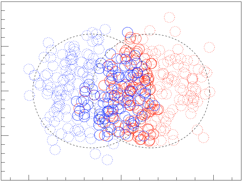
Figure 1: Simulated participant nucleon distribution (figure from Ref. [3])

Thus a simple ellipsoidal symmetry is not sufficient to describe the hydrodynamically expanding medium, not to mention that it does not describe higher order flow coefficients either. To overcome this difficulty, one can assume higher order anisotropies in the scaling variable, by redefining it as

$$s=\frac{r^{2}}{R^{2}}\left(1+\varepsilon_{2}\cos(2\phi)\right)+\frac{z^{2}}{Z^{2}}$$ (7)

with $r$ and $\phi$ being the polar coordinates in the transverse plane, while $R$ and $\varepsilon_{2}$ are in a direct relation to $X$ and $Y$. This can then be generalized to

$$s=\frac{r^{2}}{R^{2}}\left(1+\sum\limits_{n=2,3,\dots}\varepsilon_{n}\cos{n\varphi}\right)+\frac{z^{2}}{Z^{2}}$$ (8)

in the $\cos{n\varphi}$ expression a $\Psi_{n}$ $n$-th order event plane can also be introduced. Example distributions generated with this scaling variable are shown in Fig. 2. Solutions utilizing scaling variables like the above $s$ were presented in Ref. [4]. However, these solutions, as well as the ones in Ref. [1] are valid only in case of a 3D Hubble-flow, which corresponds to the lack of pressure gradients. This also means that the anisotropies will remain constant in time, which may not be the case throughout the whole evolution. In our analysis, we thus apply numerical calculations to include pressure gradients in the initial conditions, and analyze the time evolution of the anisotropies.

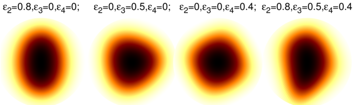
Figure 2: Initial distribution with the outlined $s$ scaling variable, for different $\varepsilon_{n}$ values.

Thus we will start the hydrodynamic evolution from the above described set of initial conditions. We would like to extract the anisotropy coefficients at later stages of the evolution, for which we need a definition. We introduced the anisotropies of density, energy density and velocity fields as follows:

$$\epsilon_{n}=\langle\cos(n\varphi)\rangle_{\rm\rho/\varepsilon/w},$$ (9)

where $w=\exp{(-v_{x}^{2}-v_{y}^{2})}$ is defined to calculate the asymmetry of velocity field. To understand the relation of the asymmetry parameters introduced by 9 to the scale variable anisotripy coefficients, $\varepsilon_{n}$’s, we checked their relation. As a first order approximation (in $\varepsilon_{n}$), we obtained

$$\epsilon_{n}=-\varepsilon_{n}/2$$ (10)

however, in a more accurate approximation the result is:

$$\epsilon_{1} \approx\frac{(\varepsilon_{2}+\varepsilon_{4})\varepsilon_{3}}{2+\sum_{n}\varepsilon_{n}^{2}}=\frac{\epsilon_{3}(\epsilon_{2}+\epsilon_{4})}{2}+\mathcal{O}(\epsilon_{n}^{4})$$ (11)

$$\epsilon_{2} \approx\frac{-\varepsilon_{2}+\varepsilon_{2}\varepsilon_{4}}{2+\sum_{n}\varepsilon_{n}^{2}}=-\frac{\epsilon_{2}}{2}+\frac{\epsilon_{2}\epsilon_{4}}{2}+\frac{1}{4}\epsilon_{2}\sum_{n}\epsilon_{n}^{2}+\mathcal{O}(\epsilon_{n}^{4})$$ (12)

$$\epsilon_{3} \approx\frac{-\varepsilon_{3}}{2+\sum_{n}\varepsilon_{n}^{2}}=-\frac{\epsilon_{3}}{2}+\frac{1}{4}\epsilon_{3}\sum_{n}\epsilon_{n}^{2}+\mathcal{O}(\epsilon_{n}^{4})$$ (13)

$$\epsilon_{4} \approx\frac{-\varepsilon_{4}+\frac{1}{2}\varepsilon_{2}^{2}}{2+\sum_{n}\varepsilon_{n}^{2}}=-\frac{\epsilon_{4}}{2}+\frac{\epsilon_{2}^{2}}{4}-\frac{1}{4}\epsilon_{4}\sum_{n}\epsilon_{n}^{2}+\mathcal{O}(\epsilon_{n}^{4})$$ (14)

this means that even if there is no $\varepsilon_{1}$ coefficient, we will still get an $\epsilon_{1}$. It is also important to note that $\varepsilon_{2}\neq 0$ and $\varepsilon_{n\neq 2}=0$ will result in a nonzero $\epsilon_{4}=\varepsilon_{2}^{2}/4$. See an example with multiple nonzero $\varepsilon_{n}$ coefficients in table 2, where we give an example how a set of $\varepsilon_{n}$ values result in a different set of $\epsilon_{n}$ values. The actual results can be accurately approximated with eqs. (12)-(14).

Example for the $\epsilon_{n}-\varepsilon_{n}$ relation. $n$ $\varepsilon_{n}$ $\epsilon_{n}$ direct calculation approximation first order estimate 1 0 0.00278 0.00298 0 2 0.1 -0.04927 -0.04869 -0.05 3 0.05 -0.02533 -0.02484 -0.025 4 0.02 -0.00769 -0.00745 -0.01

3 Numerical method

Let us now discuss how we evolve the previously defined initial conditions in time. In order to do that, we first transform the equations of (1+2 dimensional) hydrodynamics to a convective form as usual:

$$\partial_{t}{\bf Q}+\partial_{x}{\bf F}({\bf Q})+\partial_{y}{\bf G}({\bf Q})=0$$ (22)

where $\bf Q$ is calculated from the hydrodynamical fields, while $\bf F$ and $\bf G$ are functions of these, transformed from the original hydro equations. The finite volume method discussed below and introduced in Ref. [5] works for many different systems of partial differential equations (PDE’s), one just needs to determine the given functions to transform the PDE’s to the above form. This can be done in a straightforward manner, see for example Refs. [5, 6, 7, 8].

The basis of finite volume methods is to discretize the ${\bf Q}$ vector, by defining it on a space-time grid, and obtaining the discrete values by averaging in each cell. Then, we have to evaluate fluxes $\bf F$ and $\bf G$ between grid points (these are then called intercell fluxes). This is difficult, since the fluxes depend on the values of $\bf Q$, but these are defined on the grid points. Our method, outlined in Ref. [5] and used for exampe in Ref [7], is based on an accurate multi-stage (MUSTA) predictor-corrector estimation of the intercell fluxes. We discuss this method briefly in 1+1 dimensions (and with a single-component $Q$ only) – it is straightforward to generalize it to multiple spatial dimensions via operator splitting (we used the Lie type of splitting method here). In case of viscous hydrodynamics, we also used operator splitting to separate ideal and viscous fluxes.

To estimate the intercell fluxes between cells $i$ and $i+1$, we start from the $Q^{n}_{i}$ and $Q^{n}_{i+1}$ values, where $n$ represents the current time-step. Let us call these values $Q^{(0)}_{i,i+1}$, indicating that these represent a “zeroth order” estimate of the intercell values. We will then make a series of estimates in the given cell, the $l$th estimate being indicated with $Q^{(l)}_{i,i+1}$. The flux in the cell centers is then $F^{(l)}_{i,i+1}\equiv F\left(Q^{(l)}_{i,i+1}\right)$. We define an intermediate $Q$ value and flux $F$ as follows:

$$Q^{(l)}_{i+\frac{1}{2}}=\frac{1}{2}\left[Q^{(l)}_{i}+Q^{(l)}_{i+1}\right]-\frac{1}{2}\frac{\Delta t}{\Delta x}\left[F^{(l)}_{i+1}-F^{(l)}_{i}\right],\quad F_{M}^{(l)}\equiv F\left(Q^{(l)}_{i+\frac{1}{2}}\right)$$ (23)

Then our intercell flux estimate is

$$F^{(l)}_{i+\frac{1}{2}}=\frac{1}{4}\left[F^{(l)}_{i+1}+2F^{(l)}_{M}+F^{(l)}_{i}-\frac{\Delta x}{\Delta t}\left(Q^{(l)}_{i+1}-Q^{(l)}_{i}\right)\right]$$ (24)

This is the so called FORCE flux approximation. The essence of our the applied MUSTA algorithm is that now we make a new prediction, $Q^{(l+1)}_{i}$ and with that we repeat the steps and we get a better flux approximation, and with that we can make better prediction, and again better flux approximation. To make a new prediction simply we use the equations we want to solve:

$$Q_{i}^{(l+1)} =Q^{(l)}_{i}-\frac{\Delta t}{\Delta x}\left[F^{(l)}_{i+\frac{1}{2}}-F^{(l)}_{i}\right]$$ (25)

$$Q_{i+1}^{(l+1)} =Q^{(l)}_{i+1}-\frac{\Delta t}{\Delta x}\left[F^{(l)}_{i+1}-F^{(l)}_{i+\frac{1}{2}}\right]$$ (26)

We may then stop at a given $l$ value, by setting $F^{n}_{i+\frac{1}{2}}=F^{(l)}_{i+\frac{1}{2}}$. With this, we simply calculate the next time-step as

$$Q_{i}^{n+1}=Q_{i}^{n}-\frac{\Delta x}{\Delta t}\left(F^{n}_{i+\frac{1}{2}}-F^{n}_{i-\frac{1}{2}}\right).$$ (27)

where $F^{n}_{i-\frac{1}{2}}$ can also be calculated by the procedure outlined above, if we start from cells $i-1$ and $i$.

In order to complete the method, let us mention that we used the initial conditions as described above, we used non-reflective boundary conditions, and the timestep was determined adaptively via the Courant-Friedrichs-Lewy condition. We tested our method with the usual Sod shock tube and known hydrodynamic solutions as well.

4 Results

With the above outlined method, we solved the equations of nonrelativistic hydrodynamics with viscosity, as well as the equations of relativistic perfect hydrodynamics. Our goal was to investigate how various speed of sound values and various viscosity values affect the time evolution of the asymmetries.

Let us first discuss the effects of viscosity (in nonrelativistic hydro). As shown in Fig. 3 viscosity makes the disappearance of pressure anisotropies slower, and the same is in the number density. In other words, in case of nonzero viscosity the pressure asymmetries remain in the system for a longer time. This may be due to the fact that viscosity makes the flow slower, as illustrated in the first two plots of Fig. 4. As shown in the bottom plot of Fig. 3 and the third and fourth plots in Fig. 4, the effect of viscosity on the flow field is however the opposite: viscosity makes the flow anisotropies disappear faster. The reason of this may be that the viscous force contains the second spatial derivatives, thus the fluid elements with larger asymmetries feel a stronger viscous force, which means that viscosity “washes out” the anisotropies.

We also investigated the effects of a change in the speed of sound. As shown in Fig. 5, the reduction of speed of sound makes the anisotropies disappear slower. The reason for this is that pressure waves travel with the speed of sound, so the equalization of pressure is slower in case of smaller speed of sound values. This is confirmed by relativistic calculations as well. As shown in the top panels of Fig. 6, in case of a larger $\kappa$ (i.e. a smaller $c_{s}^{2}$ value) the anisotropies disappear slower, and also the cooling is slower. This also means that of course the system will freeze out later. The time evolution of the flow field is shown in the bottom panels of Fig. 6.

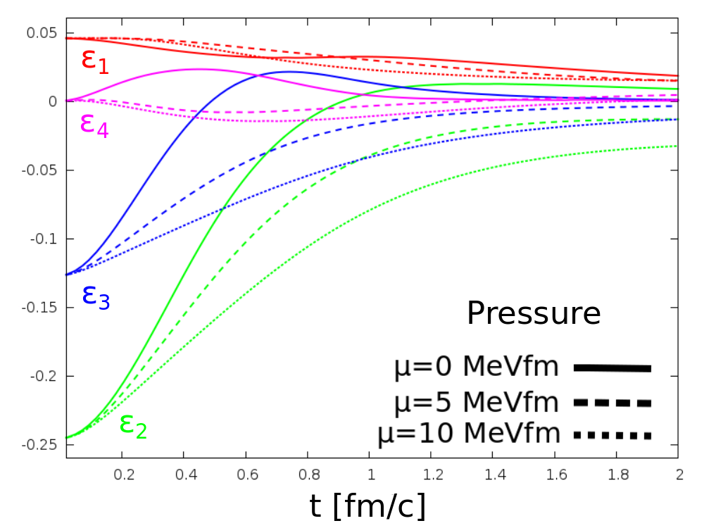
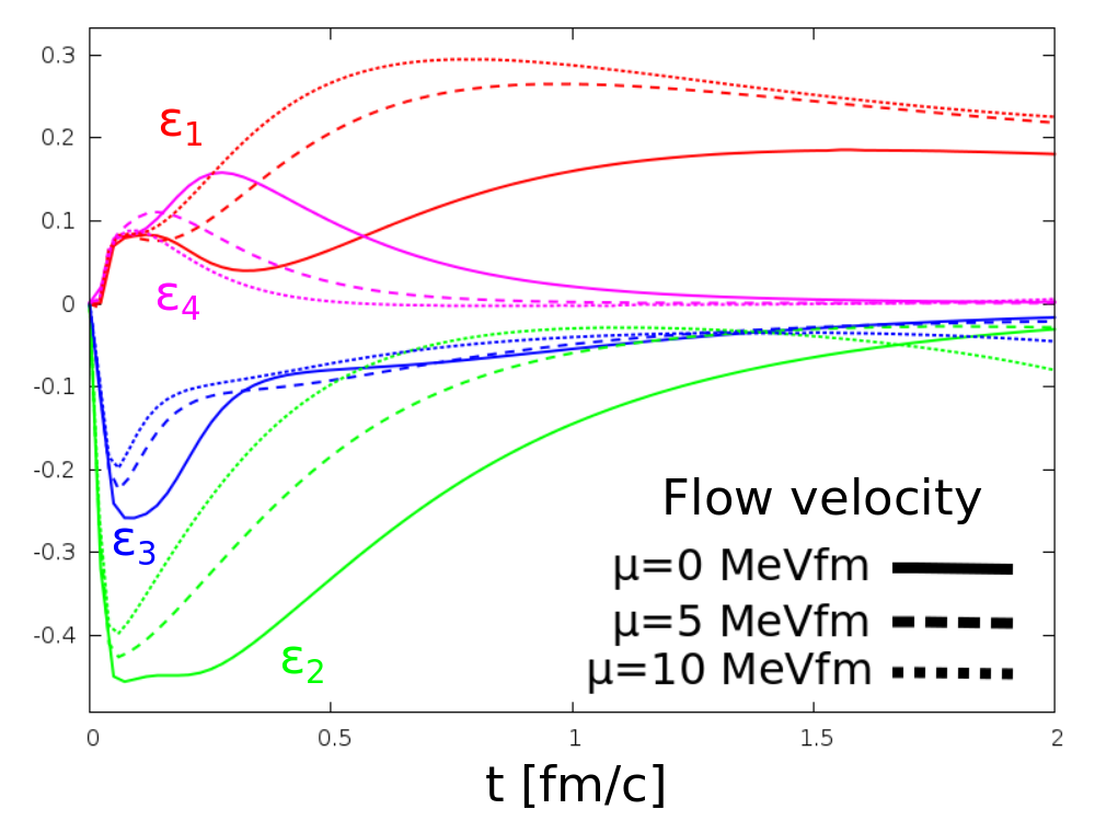
Figure 3: Time evolution of pressure anisotropies is shown in the left panel, while anisotropies in the flow field are shown in the right panel.

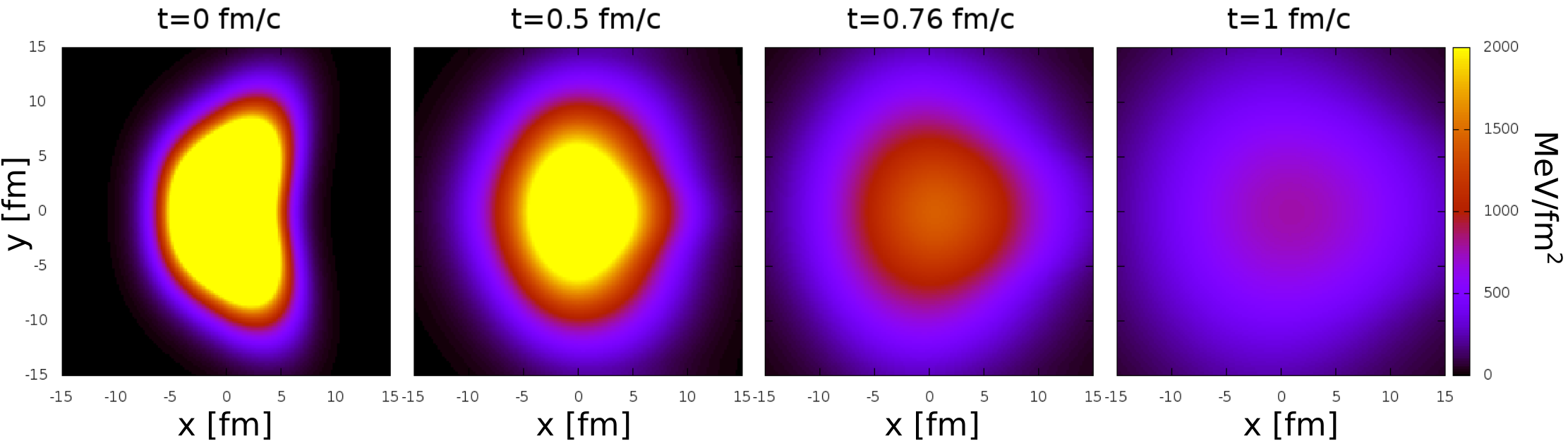
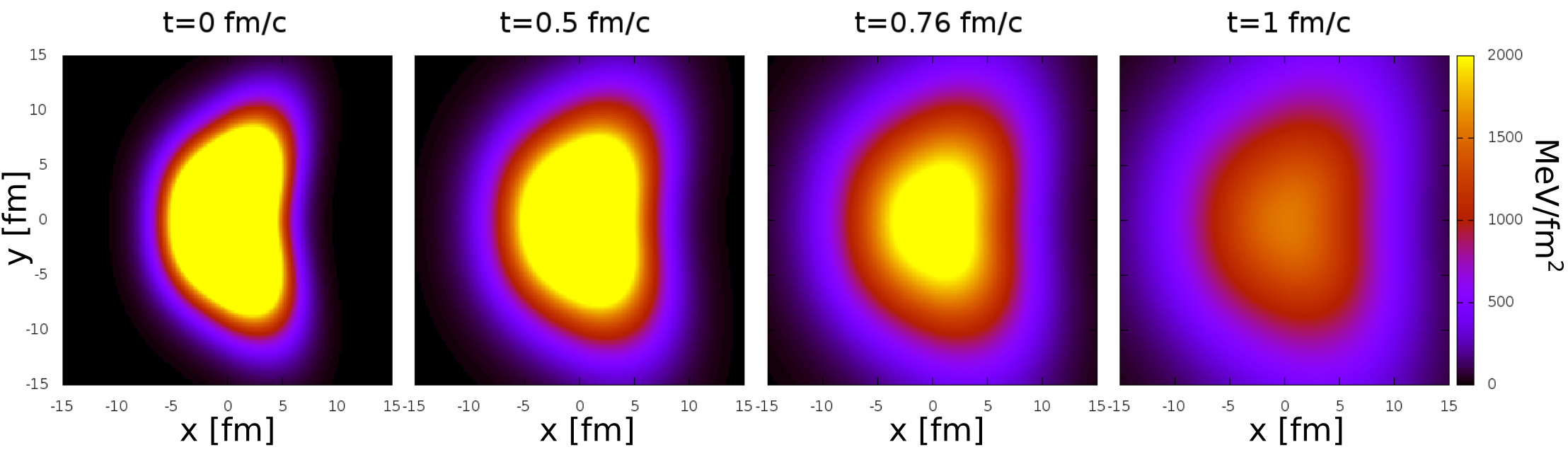
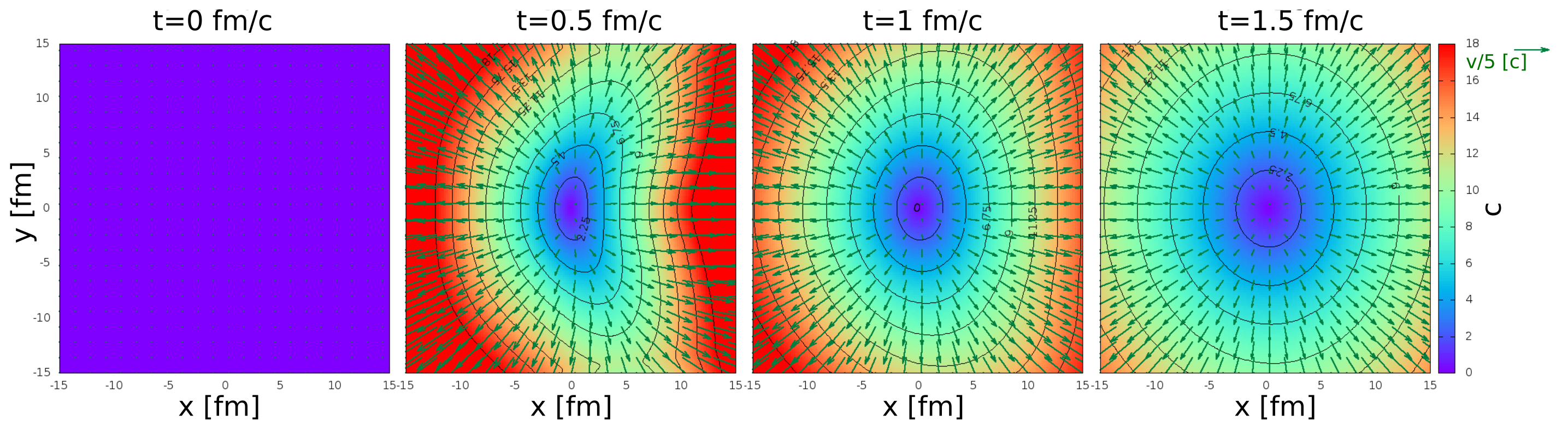
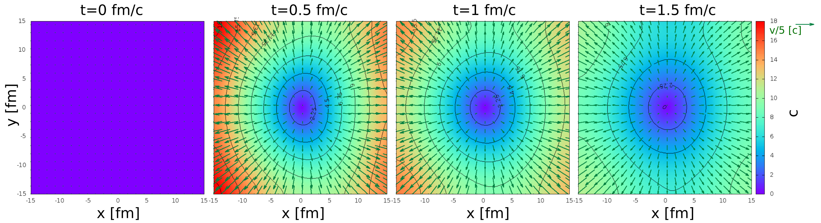
Figure 4: Time evolution of the energy density (first two rows) and of the flow field (last two rows). The first and third rows show the viscosity free case, the second and fourth rows show the viscous case with $\mu={\rm 10MeV}\cdot{\rm fm}$.

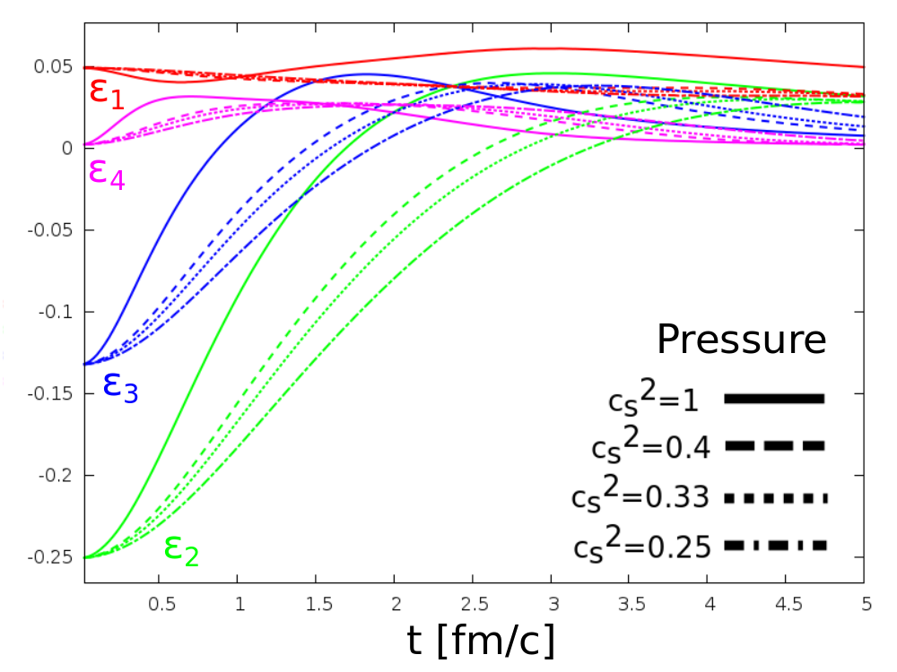
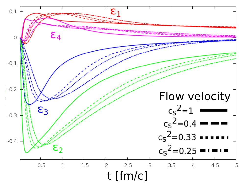
Figure 5: Time evolution of pressure anisotropies is shown in the left panel, while anisotropies in the flow field are shown in the right panel.

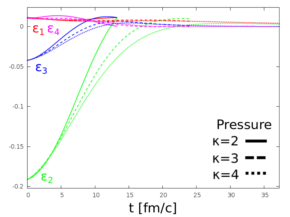
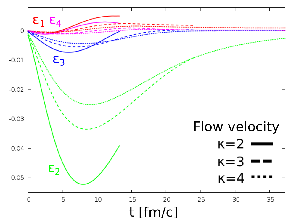
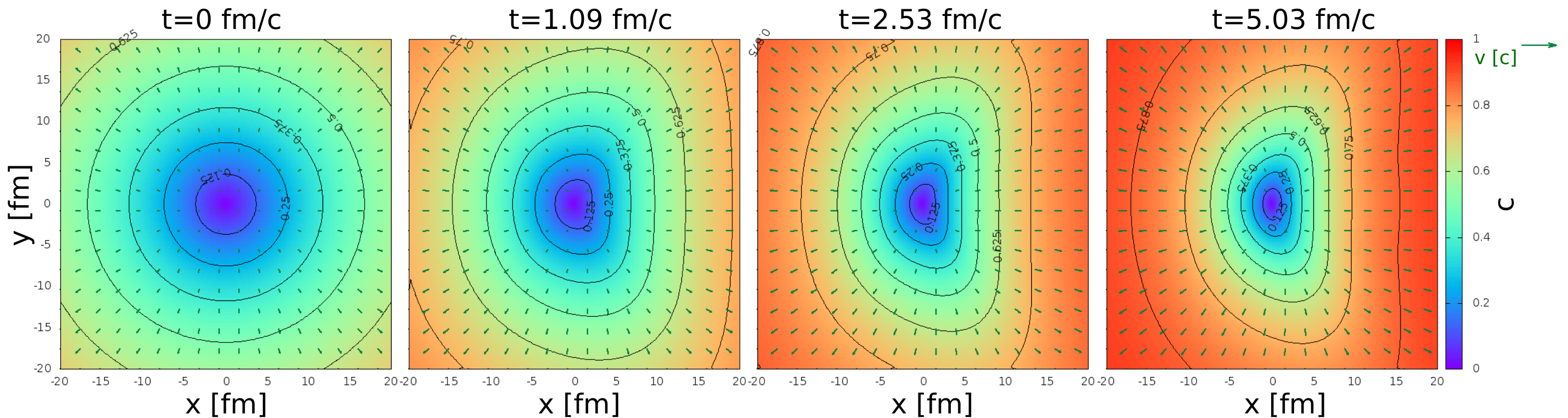
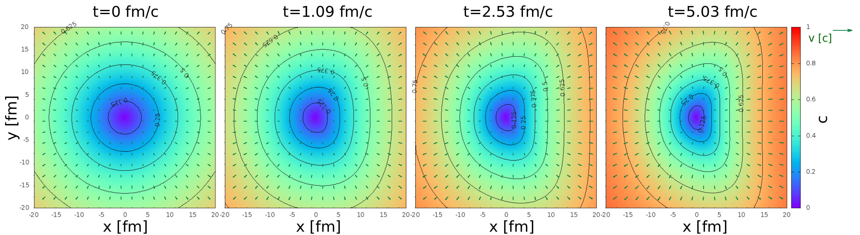
Figure 6: The time evolution of velocity field. The top row shows $\kappa=2$ case, the bottom row the $\kappa=4$ case. Time evolution of pressure anisotropies is shown in the left panel, while anisotropies in the flow field are shown in the right panel.

5 Summary

In this paper we analyzed the time evolution of the asymmetries of the QCD matter created in high energy heavy ion collisions. We utilized numerical hydrodynamics instead of exact solutions to investigate situations not describable by the presently known hydrodynamic solutions. We however did not start from the most realistic initial conditions, but started instead from an initial condition that is very similar to one described by known analytic solutions – except in pressure, where we used a pressure profile similar to the density profile given in these models. We analyzed both non-relativistic and relativistic hydrodynamics, and arrived at similar conclusions. It turns out that a stiffer equation of state, i.e. a larger speed of sound makes the pressure anisotropies disappear faster. The appearance of viscosity also makes the flow anisotropies disappear faster, however, pressure anisotropies remain in the system longer, due to the slower flow of the viscous system.

References

- [1] T. Csörgő, L. P. Csernai, Y. Hama and T. Kodama, Heavy Ion Phys. A21, 73 (2004).
- [2] T. Csörgő, S. V. Akkelin, Y. Hama, B. Lukács and Y. M. Sinyukov, Phys. Rev. C67, p. 034904 (2003).
- [3] C. Loizides, J. Nagle and P. Steinberg (2014).
- [4] M. Csanád and A. Szabó, Phys.Rev. C90, p. 054911 (2014).
- [5] E. F. Toro and V. A. Titarev, J. Comp. Phys. 216, 403 (2006).
- [6] H. Nishikawa and K. Kitamura, J. Comp. Phys. 227, 2560 (2008).
- [7] M. Takamoto and S.-i. Inutsuka, J.Comput.Phys. 230, 7002 (2011).
- [8] I. Karpenko, P. Huovinen and M. Bleicher, Comput.Phys.Commun. 185, 3016 (2014).