Energy-based Modulation for
Noncoherent Massive SIMO Systems

Abstract

An uplink system with a single antenna transmitter and a single receiver with a large number of antennas is considered. We propose an energy-detection-based single-shot noncoherent communication scheme which does not use the instantaneous channel state information (CSI), but rather only the knowledge of the channel statistics. The suggested system uses a transmitter that modulates information on the power of the symbols, and a receiver which measures only the average energy across the antennas. We propose constellation designs which are asymptotically optimal with respect to symbol error rate (SER) with an increasing number of antennas, for any finite signal to noise ratio (SNR) at the receiver, under different assumptions on the availability of CSI statistics (exact channel fading distribution or the first few moments of the channel fading distribution). We also consider the case of imperfect knowledge of the channel statistics and describe in detail the case when there is a bounded uncertainty on the moments of the fading distribution. We present numerical results on the SER performance achieved by these designs in typical scenarios and find that they may outperform existing noncoherent constellations, e.g., conventional Amplitude Shift Keying (ASK), and pilot-based schemes, e.g., Pulse Amplitude Modulation (PAM). We also observe that an optimized constellation for a specific channel distribution makes it very sensitive to uncertainties in the channel statistics. In particular, constellation designs based on optimistic channel conditions could lead to significant performance degradation in terms of the achieved symbol error rates.

I Introduction

Accurate channel state acquisition is critical to realizing many of the diversity and beamforming benefits in existing high speed communication systems. With an increasing number of antennas and operating bandwidths, the complexity and overhead of channel state acquisition grows proportionally. However, in a recent result [1, 2] for a narrowband massive SIMO system with independent and identically distributed channel coefficients at each of the receiver antennas, it was shown that one can achieve a scaling law in the number of receive antennas which is no different from that with perfect channel state information (CSI). The achievability uses only an average energy measurement across all the receiver antennas. In another recent work [3], it was shown that employing a similar energy-based scheme in a noncoherent massive wideband SIMO system leads to optimal capacity scaling when both the number of receive antennas and the bandwidth go to infinity jointly. These asymptotic characterizations suggest that when the number of antennas is large, the requirements on the channel state information acquisition may not be very stringent.

Motivated by these asymptotic results, in this work, we consider a finite number of receive antennas in a massive SIMO system and address the problem of optimizing the transmit constellation points based on an asymptotically tight and analytically tractable upper bound on the Bit Error Rate (BER) for any given SNR, under different assumptions on the knowledge of the CSI statistics. We also present robust constellation designs given imperfect knowledge of the channel statistics. Keeping in mind the fact that the channel moments can be estimated on time scales larger than those needed for estimating instantaneous phase (for which we typically need resource-consuming training sequences), in our work we investigate how many antennas we need for a certain BER performance. Through analysis and simulations, we find that the suggested schemes can outperform several existing noncoherent schemes, e.g., conventional ASK modulation, as well as pilot-based schemes, such as PAM modulation when the coherence time of the channel is small.

To the best of our knowledge, this line of work, with initial results appearing in [4], is the first to consider an energy-based encoding and decoding procedure for a noncoherent large antenna system and demonstrate its performance gains over other noncoherent and coherent schemes.

I-A Prior Work

Noncoherent communication, i.e., communication without instantaneous channel information, has attracted a lot of research due to either the difficulty of channel state acquisition, or the need for low hardware complexity and low energy consumption. The earliest incarnations of noncoherent systems were mostly motivated by the simplicity of the receiver circuitry: the use of envelope detectors can be traced back to the well-studied quadrature and square law receivers [5, 6] employed in the noncoherent detection of several well-known modulation schemes, such as Frequency-Shift Keying (FSK), Amplitude Shift Keying (ASK) [7] and Pulse Position Modulation (PPM) [8]. However, the spectral efficiency of these systems is inferior to that of their coherent counterparts. Hence, with the paucity of spectrum resources in cellular and with the advances in device manufacturing, coherent systems using phase acquisition circuitry at the receivers mostly replaced noncoherent systems.

However, as the demand for mobile data in wireless broadband communications increases dramatically every year, there is an evident trend towards higher and higher carrier frequencies and large antenna arrays [9], [10]. In these scenarios, the issues of simple circuit designs, inexpensive hardware components and energy efficiency become as crucial to system design as spectral efficiency [9, 11, 12]. While the number of RF chains goes up with an increasing number of antennas, thereby causing increased complexity and energy consumption, hardware impairments such as phase noise and I/Q imbalances also become more severe at both the transmitter and the receiver. Architectures which use simple, robust and energy efficient designs are thus important to realizing many of the performance benefits of massive MIMO.

Initial investigations on the rate loss incurred by even a small training overhead in a massive SIMO system show that in several scenarios of low SNR, high mobility, or a large line of sight (LOS) component, a noncoherent system achieves a better probability of bit error than a coherent system for the same effective rate [13]. Thus, noncoherent schemes seem to be a competitive alternative to coherent schemes in the design of practical large-antenna systems.

Within this line of research, [14] focuses on the noncoherent ML decoder and proposes signal constellation designs using a metric motivated by a union bound on the probability of error in the high SNR regime. Similar metrics, also motivated by a high SNR analysis, are presented in [15] where the worst-case chordal distance is employed to place the codewords as far apart as possible. An alternative to the ML detection of the transmitted symbols is considered in [16], where the authors consider the problem of joint channel and transmitted symbol estimation, and propose a minimum distance criterion for code design using the Generalized Likelihood Ratio Test (GLRT) in the AWGN channel at high SNR. The GLRT is necessary when the channel statistics are not known precisely and it involves maximizing the noncoherent likelihood function over all possible values of the channel statistics. While these decoders are applicable to a very general class of channels, in this work, our focus is on understanding and optimizing the performance of energy based decoders with an increasing number of antennas.

The rest of the paper is organized as follows. We present the system model in Section II, and summarize relevant work on its asymptotic characterization in Section III. Then, Section IV-A presents the constellation design problem and Section IV-B describes the solution to this problem when the channel distribution is perfectly known. Section IV-C shows how the constellation design problem can be done when only the first few moments of the fading distribution are known, and Section IV-D addresses the case when even the moments are not known perfectly. Finally, in Section V, we present plots showing the performance of the suggested schemes with representative statistics. Section VI summarizes this work.

I-B Notation

We use $[k]$ to denote the set $\{1,2,\cdots,k\}$ where $k$ is an integer. $\mathbb{C}^{n\times m}$ is the set of all complex-valued matrices of size $n\times m$. For a matrix ${\bf{H}}\in\mathbb{C}^{n\times m}$, the $(i,j)$-th element is denoted by $H_{i,j}$ and for a vector ${\bf{h}}\in\mathbb{C}^{n\times 1}$, the $i$-th element is denoted as $h_{i}$. $\operatorname{Re}(\cdot)$ and $\operatorname{Im}(\cdot)$ represent the real and imaginary terms, respectively. $\mathcal{CN}(\mu,{\bf{R}})$ represents the distribution of circularly symmetric complex Gaussian (CSCG) random vectors with mean vector $\mu$ and a covariance matrix ${\bf{R}}$. The symbol $\triangleq$ is used to denote a definition. $\mathcal{P}$ refers to a set of power levels that the transmitter uses and $n$ is used to denote the number of receive antennas. We refer to a $(K,\gamma)$ Rician fading channel as a channel with Rician fading ($K$-factor in dB units and unit second moment) and additive Gaussian noise with power $\sigma^{2}=-\gamma$ in dB.

II System Model

Consider one single antenna transmitter in a flat fading channel and a receiver with $n$ antennas, where $n$ is a large (but finite) number. The system is represented as

$${\bf{y}}={\bf{h}}x+{\bf{v}},$$ (1)

with ${\bf{y}}\in\mathbb{C}^{n\times 1}$, $x\in\mathbb{C}$, ${\bf{v}}\in\mathbb{C}^{n\times 1}$, ${\bf{h}}\in\mathbb{C}^{n\times 1}$ and each $v_{i}\sim\mathcal{CN}(0,\sigma^{2})$, $h_{i}\sim f(h)$, such that $\operatorname{E}[h_{i}]=\mu,~{}\operatorname{E}\left[|h_{i}-\mu|^{2}\right]=\sigma_{h}^{2}$, and $f(h)$ is the probability density function of the channel distribution. For normalization purposes and for notational simplicity, we also assume that $\operatorname{E}[|h_{i}|^{2}]=1$ and $\operatorname{E}[|x|^{2}]=1$ so that parameters such as long-term shadowing, path-loss and antenna gain are incorporated in the $\sigma^{2}$. Then, the average SNR per antenna at the receiver for this model is

$$\gamma\triangleq\frac{\operatorname{E}[|h_{i}|^{2}]}{\sigma^{2}}=\frac{1}{\sigma^{2}}.$$

We further assume that the density function $f(h)$ is such that, for any fixed $x\in\mathbb{C}$, the moment generating function of $|y_{i}|^{2}$, i.e., $\operatorname{E}[e^{\theta|y_{i}|^{2}}]$, exists and is twice differentiable in an interval around $\theta=0$. Many fading distributions fall within this model, e.g., Rayleigh and Rician fading [17], in which case $h_{i}\sim\mathcal{CN}(\mu,\sigma_{h}^{2})$.

Note that an important aspect of this system model, similar to many works in the massive MIMO literature, is the assumption that the channel realizations across the antennas are i.i.d. random variables. While this assumption is not typically accurate in practice, some recent measurements [18, 19, 20] suggest that, despite the statistical difference between the measured multiple antenna channels and the i.i.d. channels, most of the theoretical conclusions made under the independence assumption are still valid in real massive MIMO channels.

Motivated by our recent asymptotic results in [1, 2, 3], this work focuses on symbol-by-symbol encoding and decoding schemes that use an average energy-based transmitter and receiver design. This means that information is modulated in the power of the transmitted symbols, $|x|^{2}$, and the receiver estimates only the average power of the received signal, $\frac{||y||^{2}}{n}$. We describe this next.

II-A Transmitter architecture: energy encoder

The transmitter encodes information only in the power of the transmitted symbols, i.e., it transmits symbols with power levels from a codebook

$$\mathcal{P}=\{p_{1},p_{2},\cdots,p_{L}\},$$

where $p_{k}\in\mathbb{R_{+}},$ subject to an average power constraint

$$\frac{1}{L}\sum_{k=1}^{L}p_{k}\leq 1,$$

assuming equiprobable signaling. Here $p_{k}\in\mathcal{P}$ is the power level of the $k^{th}$ symbol and $L$ is the cardinality of $\mathcal{P}$. Note here that we do not encode information in the phase.

II-B Receiver architecture: energy decoder

Assume the user transmits a symbol whose power is the $k^{th}$ constellation point from $\mathcal{P}$, i.e, $p_{k}$. In order for the receiver to detect $p_{k}$, it only computes the following statistic

$$\frac{\|\mathbf{y}\|^{2}}{n}=\frac{\sum_{i=1}^{n}|y_{i}|^{2}}{n}\in\mathbb{R}^{+},$$ (2)

i.e., it estimates only the average received power across all its antennas. Based on its knowledge of the statistics of the channel, the receiver divides the positive real line into non-intersecting intervals or decoding regions

$$\mathcal{D}=\{\mathcal{I}_{k}\}_{k=1}^{L},$$

(each $\mathcal{I}_{k}$ corresponding to each ${p_{k}}\in\mathcal{P}$), and returns

$$\hat{k}\in\left\{\tilde{k}:\frac{\|\mathbf{y}\|^{2}}{n}\in\mathcal{I}_{\tilde{k}}\right\}.$$ (3)

The probability of error $P_{e}(p_{k})$ when the $k^{th}$ power level $p_{k}\in\mathcal{P}$ is transmitted, and the average Symbol Error Rate (SER) $P_{s}$ for any fixed constellation size $L$ are defined as

$$P_{e}(p_{k})\triangleq Pr\{\hat{k}\neq k\},~{}~{}P_{s}\triangleq\frac{1}{L}\sum_{k=1}^{L}P_{e}(p_{k}),$$ (4)

respectively, assuming equiprobable signaling.

II-C Discussion

The use of energy-detection-based transmission and decoding is motivated by the fact, proved in [2], that such an encoding and decoding method achieves the same BER as a noncoherent maximum likelihood (ML) scheme in the Rayleigh fading channel. To see this, as explained in more details in [2], assume the transmitter sends a symbol $x\in\mathbb{C}$. The log likelihood function for a noncoherent Rician fading channel, i.e., $h_{i}\sim\mathcal{CN}(\mu,\sigma_{h}^{2})$, is

$$\log f_{x}^{NC}({\bf{y}})=\frac{\|{\bf{y}}-\mu x\mathbf{1}\|^{2}}{\sigma+\sigma_{h}^{2}|x|^{2}}+n\log\left(\pi(\sigma+\sigma_{h}^{2}|x|^{2})\right),$$

and therefore, the noncoherent ML decoder is

$$\hat{k}=\operatorname{argmax}_{x:|x|^{2}=p_{k},\forall k}\log f_{x}^{NC}({\bf{y}}).$$ (5)

For $\mu=0$, i.e., Rayleigh fading, the noncoherent ML decoder depends only on $\|{\bf{y}}\|^{2}$. Thus for suitably chosen decoding regions $\mathcal{D}$, it performs as well as the ML decoder. In general for $\mu\neq 0$, energy based detectors are not optimal. However, as shown in Figure 3 for representative values for $\mu$, the SER performance gap is typically small.

The proposed architecture requires a very simple one-dimensional statistic of the received signals, which allows for a simplified RF chain design. A general noncoherent ML or coherent detector, on the other hand, requires much more complicated circuits.

III Constellation Design Optimization

We are interested in the problem of minimizing SER for any fixed constellation size $L$ and fixed $n$, i.e.,

$$\mathcal{P}^{*},\mathcal{D}^{*}= {\text{ argmin}}~{}~{}~{}~{}~{}~{}~{}\frac{1}{n}\log(P_{s})$$ (6)

$$\mbox{ subject to}~{}~{}~{}~{}\frac{1}{L}\sum_{k=1}^{L}p_{k}\leq 1,$$

$$~{}~{}~{}~{}~{}~{}~{}~{}~{}~{}~{}~{}~{}~{}~{}~{}~{}0\leq p_{k},~{}\forall k\in[n].$$

The optimization above is over all codebooks $\mathcal{P}$ and decoding regions $\mathcal{D}$. Unfortunately, this is in general a difficult problem to solve. The scope of this work is to solve a specific relaxation of this problem motivated by the large $n$ asymptotics ($n$ is large but finite) for any channel distribution that has a m.g.f. Specifically, we consider maximizing the error exponent of SER with respect to $n$, or a second-order approximation of it. Before describing the relaxation we first define the notion of the error exponent of SER with respect to $n$. Using this asymptotic characterization not only helps us make the constellation design problem tractable, but also gives us designs which work for little prior statistical characterization and decouples the effect of the number of receive antennas from the effect of the channel distribution.

III-A Error exponents

Fix any codebook $\cal P$. Define the receiver’s constellation points $r(p_{k})$ to be the value of the average received energy when the transmitter sends the $k^{th}$ power level, i.e.,

$$r(p_{k})\triangleq p_{k}+\sigma^{2}.$$

We now observe that

$$\frac{||\mathbf{y}||^{2}}{n}= \frac{||\mathbf{h}\sqrt{p_{k}}+{\bf{v}}||^{2}}{n}=\frac{||\mathbf{h}||^{2}}{n}p_{k}+\frac{||{\bf{v}}||^{2}}{n}+2\frac{\textrm{Re}(\mathbf{h}^{*}{\bf{v}})}{n}\sqrt{p_{k}},$$

so, in the limit of large $n$, due to the law of large numbers and the independence of ${\bf{h}}$ and ${\bf{v}}$, it follows that

$$\lim\limits_{n\rightarrow\infty}\frac{||\mathbf{y}||^{2}}{n}=r(p_{k}).$$

For finite $n$, the statistic $\frac{\|\mathbf{y}\|^{2}}{n}$ would deviate from the value $r(p_{k})$. To characterize this deviation, it is helpful to define

$$u_{k,i}=\left|h_{i}\sqrt{p_{k}}+\nu_{i}\right|^{2}-E\left[\left|h_{i}\sqrt{p_{k}}+\nu_{i}\right|^{2}\right]=\left|h_{i}\sqrt{p_{k}}+\nu_{i}\right|^{2}-r(p_{k})$$ (7)

as the random variation of the received energy at the $i^{th}$ antenna around its expected value $r(p_{k})$. Note that $\{u_{k,i}\}_{i=1}^{n}$ are independent realizations of the same zero-mean random variable $U_{k}\sim g_{k}(u)$ whose m.g.f. is

$$M_{k}(\theta)\triangleq\operatorname{E}[e^{\theta U_{k}}].$$ (8)

In the above, $M_{k}(\theta)$ depends on the statistics of the channel and the noise, and the power level $p_{k}$.

In [2], we derived an upper bound for the objective in (6) as follows:

$$P_{s}\leq\frac{1}{L}\sum_{k=1}^{L}\left(e^{-nI_{R,k}(d_{R,k})}+e^{-nI_{L,k}(d_{L,k})}\right),$$ (9)

where

$$I_{L,k}(d)\triangleq\sup_{\theta\geq 0}\left(\theta d-\log(M_{k}(-\theta))\right),~{}~{}~{}I_{R,k}(d)\triangleq\sup_{\theta\geq 0}\left(\theta d-\log(M_{k}(\theta))\right),$$ (10)

are defined as the left and right rate functions of $p_{k}$ respectively. In addition, $\sup_{x\in A}f(x)$, is the supremum of $f(x)$ in $A$. The decoding regions are chosen as

$${\cal I}_{k}\triangleq\left(r(p_{k})-d_{L,k},r(p_{k})+d_{R,k}\right],$$

for some $d_{L,k}$ and $d_{R,k}$. Define

$$I_{k}\triangleq\min\big{(}I_{L,k}(d_{L,k}),I_{R,k}(d_{R,k})\big{)}$$

to be the rate function of the constellation point $p_{k}$. Then, it was shown in [2] that

$$I_{e}\triangleq\lim_{n\rightarrow\infty}-\frac{\log(P_{s})}{n}=\min_{k\in[L]}I_{k},$$ (11)

i.e., the error exponent of SER, denoted as $I_{e}$, is the same as the worst rate function of the constellation points. In other words, for $n$ large enough, the probability of error performance is dominated by the constellation point with the worst rate function. Therefore, the constellation points $\mathcal{P}$ and the corresponding decoding regions $\mathcal{D}$ could be chosen in such a way as to maximize the error exponent of SER, i.e., (error exponent maximization problem)

$${\text{maximize}}~{}~{}~{}~{}~{}~{}~{}I_{e}$$ (12)

$$\mbox{subject to}~{}~{}~{}~{}~{}~{}\frac{1}{L}\sum_{k=1}^{L}p_{k}\leq 1,~{}0\leq p_{k}.$$

Observe that problem (12) is a relaxation of problem (6) for any finite $n$, since its objective function is an upper bound on the objective function of the latter. Yet, note that due to (11) this relaxation would provide an asymptotically optimal constellation with increasing $n$, even if it does not explicitly solve the SER minimization problem exactly for any finite $n$ (6). Furthermore, an interesting aspect of (12) is that it depends only on the channel distribution, and not on the number of antennas. By decoupling number of antennas from the channel distribution it allows us to study achievable SERs with large $n$ without explicitly solving (6).

In [2] we showed the following about the left and right rate functions for any $p_{k}$:

Lemma 1.

The left and right rate functions $I_{R,k}(d),I_{L,k}(d)$, respectively, of the power level $p_{k}$ enjoy the following properties:

• They satisfy

  $$\lim_{d\rightarrow 0}\frac{I_{R,k}(d)}{d^{2}}=\lim_{d\rightarrow 0}\frac{I_{L,k}(d)}{d^{2}}=\frac{1}{2\operatorname{E}[U_{k}^{2}]},~{}~{}\mbox{ where }~{}~{}U_{k}=|h\sqrt{p_{k}}+v|^{2}-p_{k}-\sigma^{2},$$

  with $h\sim f(h)$ and $v\sim\mathcal{CN}(0,\sigma^{2})$.

• They are non-negative, convex and monotonically increasing for positive $d$ for a fixed non-negative $p_{k}$, and monotonically decreasing for non-negative $p_{k}$ for a fixed positive $d$.

• It holds that $I_{L,k}(0)=I_{R,k}(0)=0$ for any non-negative $p_{k}$.

The above lemma provides important insights into the dependence of the rate functions on the power levels and channel statistics. Specifically, for a small $d$, which practically means large constellations, we can approximate the rate function using only the first few moments of the channel distribution ($E[U_{k}^{2}]$ depends on the first, second, and forth moment of the fading distribution as we explicitly show in Section IV-C). Also, for a fixed $d$, increasing $p_{k}$ leads to smaller rate functions, i.e., worse SER performance, or in other words, the constellation points that correspond to high power levels generally experience worse performance than those with low power levels for decoding regions of the same size. We now describe how these analytical properties could be used to solve for the maximum error exponent as defined in problem (12).

IV Constellation designs

IV-A Overview

In this section we consider three cases of constellation designs to maximize the error exponent in (12), where each case corresponds to a different assumption on the availability of statistical information about the channel.

• Case 1: Subsection IV-B presents a design which assumes that the encoder and decoder know perfectly the channel distribution. This constellation is denoted as $\mathcal{P}_{K,\gamma}$.

• Case 2: Subsection IV-C presents a design in which only the first four moments of the channel distribution, are perfectly known. We will show later that these four moments suffice for a near-optimal design at high rates. This constellation is denoted as $\hat{\mathcal{P}}_{K,\gamma}$.

• Case 3: Subsection IV-D presents a design in which even the latter are imperfectly known. The corresponding constellation is $\hat{\mathcal{P}}^{(a)}_{K,\gamma}$, where $a$ is the uncertainty in dB around the nominal values $K$ and SNR.

In addition to the constellation designs above, we also consider a minimum distance constellation design, denoted as $\mathcal{P}^{min}$, that was proposed in [2], which has

$$p_{k}=\frac{2(k-1)}{L-1},\mbox{ for }k\in[L]$$

with decoding regions

$$\mathcal{I}_{0}=\left[0,\frac{1}{L-1}\right],~{}\mathcal{I}_{k}=\left[\frac{2k-3}{L-1},\frac{2k-1}{L-1}\right]~{}\forall k\in\{2,\cdots,L-1\},~{}\mathcal{I}_{L}=\left[2-\frac{1}{L-1},\infty\right].$$

We now describe each of the above constructions.

IV-B Perfect knowledge of channel distribution

We first discuss the constellation design with perfect knowledge of the channel distribution at the receiver. Since the exact channel distribution is known, $M_{k}(\theta)$ is also known at the receiver and transmitter for any chosen $p_{k}$. Then, (12) can be written as

$$\underset{\{p_{k},d_{L,k},d_{R,k}\}_{{k}\in[L]}}{\text{maximize}} \min_{k\in[L]}\big{(}I_{L,k}(d_{L,k}),I_{R,k}(d_{R,k})\big{)}$$ (13)

$$~{}0\leq p_{1}<p_{2}<\cdots<p_{L},$$

$$d_{L,k}\geq 0,~{}d_{R,k}\geq 0,$$

$$\frac{1}{L}\sum_{k=1}^{L}p_{k}\leq 1.$$

assuming decoding regions of the form ${\cal I}_{k}=(r(p_{k})-d_{L,k}~{},r(p_{k})+d_{R,k}],$ where for simplicity we assume that $d_{L,1}=d_{R,L}=\infty$.

  function: $[t^{*},\mathcal{P}^{*}]$ = Bisection( )   $t_{l}=0,t_{u}=\infty$   repeat      $t=\frac{t_{l}+t_{u}}{2}$      $[\mathcal{P},S_{t}]$ = ConstellationDesign( t )      If   $(S_{t}<1)$: $t_{l}=t$;   else   $t_{u}=t$   until $|t_{u}-t_{l}|<\epsilon$ and $|S_{t}-1|<\epsilon$   return  $\mathcal{P}^{*}=\mathcal{P};$ $t^{*}=t;$

Algorithm 1 Bisection algorithm

Algorithm 2 describes in detail how to get the solution of the optimization problem (LABEL:eq:relaxedproblem) and a detailed proof is presented in Appendix A. To exemplify the procedure and provide an intuitive argument for the validity of the suggested construction we consider the case with $L=4$ shown in Figure 1. The design is based on the following two properties that follow from Lemma 1:

1. Both $I_{L,k}(d)$ and $I_{R,k}(d)$ are non-negative and monotonically increasing functions of $d$ for a fixed $p_{k}$. This means that increasing the size of the decoding regions always helps to increase the resulting rate functions, and therefore increase the minimum amongst them.

2. Both $I_{L,k}(d)$ and $I_{R,k}(d)$ are monotonically decreasing functions of $p_{k}$ for a fixed $d$.

Figure 1: Example of the decoding regions using $L=4$

Based on these two properties, we have the following sequential construction: assume there exists a constellation with error exponent $t^{*}$ that satisfies the power constraint. This means that the left and right rate functions of all the constellation points at the receiver are at least $t^{*}$. To find this constellation choose first the minimum possible value for $p_{1}$. Then, choose the boundary of the decoding region to the right of $r(p_{1})=p_{1}+\sigma^{2}$, i.e., $c_{1}$, as show in Figure 1, such that the right rate function of $r(p_{1})$, $I_{R,1}(c_{1}-r(p_{1}))$, is at least $t^{*}$ on the boundary. Then, choose the smallest $p_{2}$ such that $r(p_{2})>c_{1}$ and the left right rate function of $r(p_{2})$, $I_{L,2}(r(p_{2})-c_{1})$, is at least $t^{*}$. Note that choosing a higher $p_{2}$ is always an option but this will lead to a design that uses more power than necessary. We perform this procedure sequentially until we find $p_{L}$. Then we check if the average power constraint is satisfied. If that is the case, the assumption that there exists a constellation with error exponent at least $t^{*}$ that satisfies the power constraint was correct. If not, we should discard this constellation, decrease $t^{*}$ and repeat the procedure. Proof that this procedure gives the optimal error exponent is presented in Appendix A.

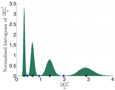
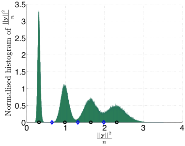
Figure 2: Example of the histogram of $\frac{||{\bf{y}}||^{2}}{n}$ for $n=100$ antennas for $\mathcal{P}_{K,\gamma}$ and $\mathcal{P}^{min}$

For $L=4$, Figures 2-(a) and 2-(b) show the normalized empirical histogram of the received statistic $\frac{||{\bf{y}}||^{2}}{n}$ in a Rayleigh fading channel of the suggested constellation: $\mathcal{P}_{K,\gamma}$ and $\mathcal{P}^{min}$. The circles and diamonds on the x-axis show the $r(p_{k})$ and the $c_{k}$ (boundaries of the decoding regions) respectively. Observe that for the $\mathcal{P}^{min}$ constellation there is a significant overlap in the histogram and therefore the receiver experiences significant symbol error rates. Also, observe that as $p_{k}$ increases, the variation around $r(p_{k})$ also increases, due to the special nature of the energy detector at the receiver.

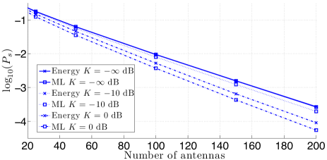
(a) Comparison of Energy and ML decoder in Rician fading with $\gamma=10$ dB

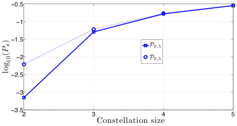
(b) $K=0$ dB, $\gamma=5$ dB

Figure 3: (a) Comparison of the energy decoder with the noncoherent ML decoder in Rician fading, (b) Comparison of $\mathcal{P}_{K,\gamma}$, $\hat{\mathcal{P}}_{K,\gamma}$ as a function of the constellation size $L$ in Rician fading

Furthermore, Figure 3 shows a numerical comparison of the SER of two systems that transmit using the same codebook $\mathcal{P}$ in Rician fading, but with different decoders; the first system uses the decoder in (3) and the decoding regions resulting from the above procedure, and the second system uses the ML noncoherent decoder (5). Observe that there is no difference in the performance of the two systems in Rayleigh fading. Moreover, even in Rician fading with a relatively strong LOS component, the difference in performance is small. This suggests that energy decoders can roughly match the performance of optimal decoder structures even when the fading distribution has a non-trivial LOS component.

      $[t^{*},\mathcal{P}^{*}]$ = Bisection( );       function: $\mathcal{P}$ = ConstellationDesign( t )   $p_{1}=0;$ $d_{L,1}=\infty;$ $d_{R,L}=\infty;$   for $k=1,2,3,\cdots,L$ do      if $k=1$ then         $p_{1}=0$      else         Find the smallest $p_{k}>p_{k-1}+d_{R,k-1}$ such that $I_{L,k}(p_{k}-p_{k-1}-d_{R,k-1})=t$         $d_{L,k}=p_{k}-p_{k-1}-d_{R,k-1}$      end if      if $k\neq L$ then         Find the smallest $d_{R,k}>0$ such that $I_{R,k}(d_{R,k})=t$      end if      $\mathcal{I}_{k}=[p_{k}+\sigma^{2}-d_{L,k},p_{k}+\sigma^{2}+d_{R,k}]$   end for   $\mathcal{P}=[p_{1},p_{2},\cdots,p_{L}],S_{t}=\frac{1}{L}\sum_{k=1}^{L}p_{k}$ , $\mathcal{D}=\{\mathcal{I}_{k}\}^{L}_{k=1}$   return  $\mathcal{P},\mathcal{D},S_{t}$   end ConstellationDesign

Algorithm 2 Constellation design: Perfect channel distribution knowledge

IV-C Perfect knowledge up to the forth channel moment

The constellation design presented above assumes that the receiver knows exactly the channel statistics. This may not be realistic in a practical scenario. In this section, we relax this assumption and consider the scenario in which the encoder and decoders only know the first few moments of the channel distribution, i.e., up to the fourth channel moment. The latter is especially important since determining the exact small-scale fading channel models in some cases, such as millimeter wave frequencies, is still ongoing research, and may not be reliably known beyond the first few moments. Moreover, the first few moments of the underlying channel distribution could potentially be estimated more efficiently (i.e., on large time scales) without the need for resource-consuming training sequences.

To see why the knowledge of the first four moments is enough to design good constellations, let $h=h_{re}+jh_{im}$, where $h_{re},h_{im}\in\mathbb{R}$. Using Lemma 1 leads to

$$I_{R,k}(d_{R,k})\approx\tilde{I}_{R,k}(d_{R,k})\triangleq\frac{d_{R,k}^{2}}{2s(p_{k})},~{}~{}I_{L,k}(d_{L,k})\approx\tilde{I}_{L,k}(d_{L,k})\triangleq\frac{d_{L,k}^{2}}{2s(p_{k})},$$ (14)

for small $d_{R,k}$ and $d_{L,k}$, with $s(p_{k})\triangleq\operatorname{E}[U_{k}^{2}]=\alpha_{1}p_{k}^{2}+\alpha_{2}p_{k}+\alpha_{3}$, and

$$\negmedspace\alpha_{1}\triangleq\operatorname{E}[h_{re}^{4}]+\operatorname{E}[h_{im}^{4}]+2\operatorname{E}[h_{re}^{2}]\operatorname{E}[h_{im}^{2}]-1,~{}\alpha_{2}\triangleq 2\sigma^{2},~{}\alpha_{3}\triangleq\sigma^{4}.$$

These expressions follow from the Gaussianity of the noise and the fact that the noise and the channel are independent and that the noise is zero mean. Observe that this approximation depends only on the first, second and fourth moment of the channel distribution. For example, in the case of Rician fading with K-factor equal to $K$ and second moment equal to $1$, it can be shown that

$$\operatorname{E}[U_{k}^{2}]=\sigma^{4}+2p_{k}\sigma^{2}+\frac{(1+2K)}{(1+K)^{2}}p_{k}^{2},$$

which means that $\alpha_{1}=\frac{1+2K}{(1+K)^{2}}.$

Substituting the objective function of (LABEL:eq:relaxedproblem) with (14) leads to the following optimization problem

$$\underset{\{p_{k},d_{L,k},d_{R,k}\}_{{k}\in[L]}}{\text{maximize}} \min_{k\in[L]}\big{(}\tilde{I}_{L,k}(d_{L,k}),\tilde{I}_{R,k}(d_{R,k})\big{)}$$ (15)

$$~{}0\leq p_{1}<p_{2}<\cdots<p_{L},d_{L,k}\geq 0,d_{R,k}\geq 0$$

$$\frac{1}{L}\sum_{k=1}^{L}p_{k}\leq 1.$$

Note that the objective of problem (LABEL:eq:relaxedproblem) has been substituted in (LABEL:eq:relaxedproblem3) with an expression which is still non-negative and non-decreasing in $d$ for a fixed $p_{k}$ and non-increasing in $p_{k}$ for a fixed $d$; i.e., all the properties and arguments that led to Algorithm 2 are still valid. Thus, the approach of solving this problem is similar to the one presented in Section IV-B, with the only difference being that both $\tilde{I}_{L,k}(d_{L,k})$ and $\tilde{I}_{R,k}(d_{R,k})$ exhibit an easily-interpretable dependence on $p_{k}$ and $d_{L,k},d_{R,k}$. Algorithm (3) contains the simplified algorithm and Appendix B shows the detailed proof.

      $[t^{*},\mathcal{P}^{*}]$ = Bisection( );       function: $\mathcal{P}$ = ConstellationDesign( t )   $p_{1}=0;$ $d_{L,1}=\infty;$ $d_{R,L}=\infty;$   $d_{R,k}=\sqrt{2ts(0)};$   for $k=2,3,\cdots,L$ do      Find the smallest $p_{k}>p_{k-1}$ such that $\frac{(p_{k}-p_{k-1}^{*})^{2}}{2\left(\sqrt{s(p_{k})}+\sqrt{s(p_{k-1}^{*})}\right)^{2}}=t;$      if $k\neq L$ then         $d_{R,k}=\sqrt{2ts(p_{k})};$      end if      $d_{L,k}=\sqrt{2ts(p_{k})};$      $\mathcal{I}_{k}=[p_{k}+\sigma^{2}-d_{L,k},p_{k}+\sigma^{2}+d_{R,k}];$   end for   end ConstellationDesign   $\mathcal{P}=[p_{1},p_{2},\cdots,p_{L}];$   return  $\mathcal{P},\mathcal{D}$;

Algorithm 3 Constellation design: Perfect knowledge of the first, second, fourth moments

Note that the suggested design leads to an algorithm which can be employed in very general channel models even when there is no knowledge of the underlying channel distribution, and that the approximation gets better as $L$ increases. This is because, as $L$ increases, the transmitted powers are packed closer together, the decoding regions (i.e., $\{d_{R,k},d_{L,k}\}$) get smaller, and thus the approximation (14) gets tighter. Figure 3-(b) shows this numerically with $\mathcal{P}_{K,\gamma}$ and $\hat{\mathcal{P}}_{K,\gamma}$ as a function of the constellation size $L$ in Rician fading with $K=0$ dB and $\gamma=5$ dB. We see that, with increasing constellation sizes, the approximation (14) gets tighter, which means that both designs lead to similar error exponents, and to approximately the same SER.

IV-D Robust constellation design

Assuming perfect knowledge of the channel distribution or even its first few moments may not be realistic due to changing propagation environments associated with user mobility and estimation errors. This motivates the need for designs which take into account uncertainties in the channel statistics. We build upon the design principles laid out in the previous sections to develop a design that performs well even in the face of channel uncertainties.

To exemplify the suggested approach, we are going to assume that the terminals have estimated the first few moments of the underlying channel distribution up to some bounded uncertainty. We want to find a constellation that could work well for all channels with moments inside their uncertainty region. Recall that

$$\operatorname{E}\left[U_{k}^{2}\right]=s(p_{k})=\alpha_{1}p_{k}^{2}+\alpha_{2}p_{k}+\alpha_{3},$$

where $a_{2}=2\sigma^{2}$ and $a_{3}=\sigma^{4}$. Thus, for a fixed $p_{k}$, $\operatorname{E}\left[U_{k}^{2}\right]$, and hence the rate function approximation depends on the channel and noise statistics only through $\alpha_{1}$ and $\sigma$. We then define the following set

$$\mathcal{F}=\{(\alpha_{1},\sigma):\alpha_{\min}<\alpha_{1}<\alpha_{\max},\sigma_{\min}<\sigma<\sigma_{\max}\},$$

and note that for each $f=(\tilde{\alpha}_{1},\tilde{\sigma})\in\mathcal{F},$ we can define

$$s_{f}(p)\triangleq\tilde{\alpha}_{1}p^{2}+\tilde{\alpha}_{2}p+\tilde{\alpha}_{3},$$

where $\tilde{\alpha}_{2}=2\tilde{\sigma}^{2},\tilde{\alpha}_{3}=\tilde{\sigma}^{4}$.

Then, in order to maximize the approximate worst-case rate function for all possible channels inside the uncertainty region, we modify problem (LABEL:eq:relaxedproblem3) in the following way:

$$\underset{\{p_{k},d_{L,k},d_{R,k}\}_{{k}\in[L]}}{\text{maximize}} \min_{f\in\mathcal{F},k\in[L]}\Bigg{(}\frac{d_{L,k}^{2}}{s_{f}(p_{k})},\frac{d_{R,k}^{2}}{s_{f}(p_{k})}\Bigg{)}$$ (16)

$$~{}0\leq p_{1}<p_{2}<\cdots<p_{L},d_{L,k}\geq 0,d_{R,k}\geq 0$$

$$\frac{1}{L}\sum_{k=1}^{L}p_{k}\leq 1.$$

In Appendix C we show how to solve problem (LABEL:eq:relaxedproblem3a) and design a constellation which maximizes the error exponent for all statistics in $\mathcal{F}$. The main difference between this design as compared to the previous two algorithms is the need for using power levels and decoding regions which would work well for any channel statistics inside the bounded uncertainty of the channel’s moments. To satisfy this, the consecutive power levels and decoding regions are generally spread out as far apart as the worst channel requires. Note also that if there is no uncertainty, Algorithm 4 reduces to Algorithm 3. An important aspect of this approach is that problem (LABEL:eq:relaxedproblem3a), in contrast to the problems (LABEL:eq:relaxedproblem) and (LABEL:eq:relaxedproblem2), may be infeasible. Such an example is presented below.

      $[t^{*},\mathcal{P}^{*}]$ = Bisection( );       function: $\mathcal{P}$ = ConstellationDesign( t )   $p_{1}=0;$ $c_{0}=-\infty$; $c_{L}=\infty$;   for $k=1,2,\cdots,L-1$ do      $c_{k}=\sup_{f\in\mathcal{F}}\left(\sigma^{2}+t\sqrt{s_{f}(p_{k})}\right)+p_{k};$      Find the smallest $p_{k+1}>p_{k}$ such that $p_{k+1}-c_{k}-\sup_{f\in\mathcal{F}}\left(t^{*}\sqrt{s_{f}(p_{k+1})}-\sigma^{2}\right)\geq 0;$      $\mathcal{I}_{k}=[c_{k-1},c_{k}];$   end for   $\mathcal{I}_{L}=[c_{L-1},c_{L}];$   $\mathcal{P}=[p_{1},p_{2},\cdots,p_{L}];$   return  $\mathcal{P}=[\mathcal{P},\mathcal{I}_{1},\cdots,\mathcal{I}_{L}]$;   end ConstellationDesign

Algorithm 4 Constellation design: Robust constellation design

IV-D1 Infeasibility of the robust constellation design problem

In this section we present a simple example that shows that, for a fixed average power constraint $P$, a very high uncertainty on the channel statistics could lead to infeasibility in the robust constellation design problem (Section IV-D). Consider the case of constructing a constellation with $L=2$, an uncertainty region $\sigma^{2}\in(\epsilon,\frac{1}{\epsilon})$ for some $\epsilon>0$ and perfectly known $\alpha_{1}=1$ for simplicity (the case of Rayleigh fading). Fix $t^{*}>0$. Then, based on Algorithm 4 we choose $p_{1}=0$ and $c_{1}=\frac{1}{\epsilon}+\frac{t^{*}}{\epsilon}$. We next choose $p_{2}$ to be the smallest $p>0$ that satisfies

$$\negmedspace p-\frac{1+t^{*}}{\epsilon}-\sup_{\sigma^{2}\in(\epsilon,\frac{1}{\epsilon})}\left(t^{*}\sqrt{p^{2}+2\sigma^{2}p+\sigma^{4}}-\sigma^{2}\right)\geq 0\Leftrightarrow p-\frac{1+t^{*}}{\epsilon}-\sup_{\sigma^{2}\in(\epsilon,\frac{1}{\epsilon})}\left(t^{*}p+\sigma^{2}(t^{*}-1)\right)\geq 0.$$

If $t^{*}\geq 1$, then $p\geq t^{*}p+2\frac{t^{*}}{\epsilon}$ which is impossible, and if $t^{*}<1$, then $p\geq\frac{1+t^{*}}{1-t^{*}}\frac{1}{\epsilon}-\epsilon$. Thus, the smallest choice of $p_{2}$ that can be chosen is $p_{2}=\frac{1+t^{*}}{1-t^{*}}\frac{1}{\epsilon}-\epsilon.$ In this case, since

$$p_{1}+p_{2}\leq 2P\Rightarrow\frac{1+t^{*}}{1-t^{*}}\frac{1}{\epsilon}-\epsilon<2P,$$

it follows that, no matter how small $t^{*}$ is, if the uncertainty is so large such that $2P<\frac{1}{\epsilon}-\epsilon$, the robust design problem will be infeasible.

V Numerical examples

This section contains simulation studies which demonstrate and compare the performance of all the constellation designs proposed in this work. In the following sections, for the constellation designs which depend on an underlying channel, i.e., $\mathcal{P}_{K,\gamma},\hat{\mathcal{P}}_{K,\gamma},\hat{\mathcal{P}}^{(a)}_{K,\gamma}$, the $(K,\gamma)$ channel is referred to as the nominal channel, whereas any other channel is referred to as a mismatched channel.

V-A Comparison with a pilot-based system with PAM and a noncoherent system with ASK

Consider a block-fading Rician fading channel $h_{i}\sim\mathcal{CN}(\mu,\sigma^{2})$ with coherence time $T$ and with $n$ antennas at the receiver. We assume that both the transmitter and the receiver know the channel statistics but not the exact channel realization.

In the first numerical example we compare the proposed $\mathcal{P}_{K,\gamma}$ with the ASK constellation, and with a system that uses a PAM constellation (referred to as PAM system) assuming a binary reflected Gray Code (BRGC) [17]. In the PAM system the transmitter uses the first $T_{l}$ slots of each coherence interval to transmit pilot symbols. Based on the received signals in these slots, the receiver derives the MMSE channel estimates $\{\hat{h}_{i}\}$ at the end of the $T_{l}$ learning slots. Using these estimates it decodes the symbols transmitted during the remaining $T-T_{l}$ slots of the coherence interval. Note that, assuming a constellation size of $L$, the effective rate of such a system is

$$\frac{T-T_{l}}{T}\log_{2}(L).$$

The noncoherent system that uses ASK i.e., amplitudes that are equally spaced apart, performs decoding using an energy-based ML receiver.

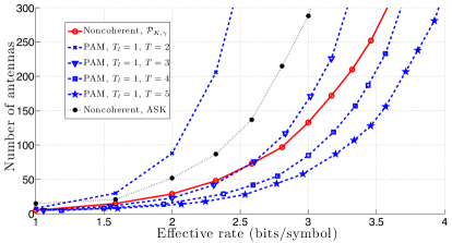
(a) $K=-\infty$ dB, $\gamma=10$ dB

(b) $K=0$ dB, $\gamma=10$ dB

(c) $K=-5$ dB, $\gamma=10$ dB

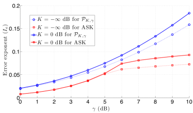
(d) $L=4$

Figure 4: (a)-(c) Minimum $n$ for a target BER $=10^{-3}$, (d) Error exponents of ASK and $\mathcal{P}_{K,\gamma}$

Figures 4-(a) to 4-(c) plot the minimum number of antennas needed to achieve an uncoded $\mbox{BER }=10^{-3}$ for different $K$ and $\gamma=10$ dB for different coherence times $T$. We make the following observations:

• First, our noncoherent constellation design performs significantly better than the system with an ASK constellation. For example, in Rayleigh fading our constellation needs approximately half the number of antennas to achieve the same BER performance.

• Second, even in the case of high $K$ (4-(b),4-(c)), which is known to all the receivers, our system performs better than the noncoherent PAM system (i.e., $T_{l}=0$) which exploits the phase of the LOS component of the channel. Note that this is not the case with our system which only uses the $K-$factor to decode the symbols.

Note that Figure 4-(a) does not show the performance of the PAM system since in Rayleigh fading the latter cannot reach the BER target for any number of antennas as the phase of the transmitted symbol is completely destroyed. We also observe that, for short coherence times, the proposed constellation design still requires a smaller number of antennas to reach the BER threshold compared to the PAM system with $T_{l}=1$. On the other hand, for higher coherence times, the PAM system achieves better performance since the gains of learning are more than the corresponding decrease in the effective rate. Yet, observe that for small effective rates, e.g., $1-2$ bits/symbol, the additional number of antennas needed by the energy-based system to achieve the same BER as PAM is not more than $20$. This shows that even a simple energy-based architecture design at the receiver, which requires only envelope detectors, could be enough to transmit information as reliably as a typical pilot-based system, especially in channels with small coherence times and high LOS, without the need for significantly more antennas.

Figure 4-(d) plots the error exponent $I_{e}$ for different values of $\gamma$, and Rician channels with $K=\{\infty,0\}$ dB and $L=4$, for two noncoherent systems that use ASK and $\mathcal{P}_{K,\gamma}$. We observe that for all channel conditions, our noncoherent constellation design achieves a much higher $I_{e}$ than the ASK constellation. Also, for high SNR, the error exponent that uses the ASK constellation is not increasing as fast as the system with $\mathcal{P}_{K,\gamma}$. This is due to the fact that the power levels are fixed, and do not adapt to the channel conditions. This is not the case with the $\mathcal{P}_{K,\gamma}$ constellation.

V-B SER performance comparison of $\mathcal{P}_{K,\gamma}$, $\hat{\mathcal{P}}_{K,\gamma}$, $\mathcal{P}^{min}$, ASK

(a) $K=-\infty$ dB, $\gamma=5$ dB

(b) $K=-\infty$ dB, $\gamma=10$ dB

Figure 5: SER performance comparison of $\mathcal{P}_{K,\gamma}$, $\hat{\mathcal{P}}_{K,\gamma}$, $\mathcal{P}^{min}$, ASK.

In the second numerical example (Figure 5) we present, as a function of $n$, a numerical SER estimate for a $3-$bit constellation ($L=8$) for channels with $K=-\infty$ dB, i.e., Rayleigh fading and $\gamma=\{5,10\}$ dB. We consider the following constellations: $\mathcal{P}_{K,\gamma}$, $\hat{\mathcal{P}}_{K,\gamma}$, $\mathcal{P}^{min}$ and ASK. As expected, $\mathcal{P}_{K,\gamma}$ achieves better SER performance than all the remaining designs. Yet, the difference of the approximate design $\hat{\mathcal{P}}_{K,\gamma}$ from $\mathcal{P}_{K,\gamma}$ is not significant, especially at low SNR. Also, the minimum distance design $\mathcal{P}^{min}$ is significantly worse than any other design, except for very low SNRs, where the gap in the performance is smaller.

(a) $K=-11$ dB, $\gamma=9$ dB

(b) $K=-9$ dB, $\gamma=9$ dB

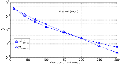
(c) $K=-9$ dB, $\gamma=11$ dB

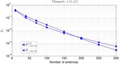
(d) $K=-11$ dB, $\gamma=11$ dB

Figure 6: SER performance of the robust constellation designs in mismatched channel

V-C Performance of the robust constellation designs on the nominal and mismatched channels

In the third numerical example we demonstrate the inefficiency of the $\hat{\mathcal{P}}_{K,\gamma}$ constellation in a mismatched channel and the ability of $\hat{\mathcal{P}}^{(a)}_{K,\gamma}$ to sustain good performance. Specifically, we consider $L=8$, the case of a user with $2-$dB of uncertainty in both $K$ and $\gamma$ values and that the center of the uncertainty interval corresponds to the $(-10,10)$ channel. This channel is approximately Rayleigh fading ($K$ is very low) with a high SNR value. In Figures 6-(a), 6-(b), 6-(c), 6-(d) we plot the Monte Carlo SER estimate of the $\hat{\mathcal{P}}_{-10,10}$ and $\hat{\mathcal{P}}^{(2)}_{-10,10}$ designs on the $\{(-9,9),(-9,11),(-11,9),(-11,11)\}$ channels respectively. Observe the huge performance loss that occurs due to the overestimation of the SNR. Smaller performance loss is observed due to the uncertainty on the value of $K$, or when the SNR is underestimated.

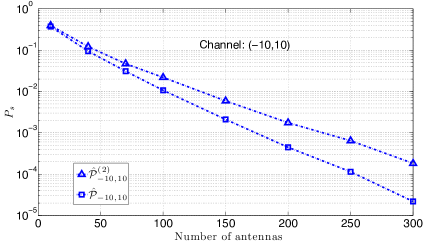
(a) $K=-10$ dB, $\gamma=10$ dB

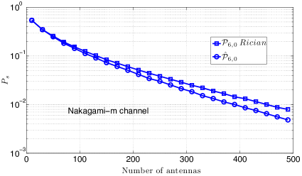
(b) $K=6$ dB, $\gamma=0$ dB

Figure 7: (a) SER performance of the robust constellation designs in nominal channel (b) Nakagami-m fading channel

Figure 7-(a) presents the SER performance of $\hat{\mathcal{P}}^{(2)}_{-10,10}$ and $\hat{\mathcal{P}}_{-10,10}$ in the $(-10,10)$ channel to show that even with nominal statistics, the performance of the robust design is close to that of the design that is explicitly optimized for the nominal statistics. This shows that the maximum performance loss due to the robust design compared to a constellation optimized for a known channel is tolerable, especially considering the fact that not taking into account the uncertainty could lead to a significant performance deterioration as presented in the previous numerical example.

V-D Performance on a Nakagami-$m$ fading channel

We now show an example in which using $\mathcal{P}_{K,\gamma}$ designed for a Rician fading channel leads to a worse performance compared to a $\hat{\mathcal{P}}_{K,\gamma}$ in a Nakagami-$m$ fading channel. This shows that not taking into account the uncertainty in the channel distribution, and over-optimizing the constellations for the Rician channel, could lead to worse performance than a much simpler constellation design which is based only on the first four moments of the channel. Specifically, consider the case of a channel for which it holds that

$$\operatorname{E}[h_{i}]=\sqrt{\frac{K}{K+1}},~{}E\left[|h_{i}|^{2}\right]=1,E\left[\left|h_{i}-\sqrt{\frac{K}{1+K}}\right|^{2}\right]=\frac{1}{1+K}.$$

This channel could correspond to a Rician channel, i.e., $h_{i}\sim\mathcal{CN}\left(\sqrt{\frac{K}{K+1}},\frac{1}{1+K}\right),$ or a Nakagami-m channel with $\Omega=1$ and $m$ such that $\frac{\Gamma(m+\frac{1}{2})}{\Gamma(m)}\frac{1}{\sqrt{m}}=\sqrt{\frac{K}{K+1}}.$ Figure 7-(d) plots $P_{s}$ for $\gamma=0$ dB and $K=6$ dB in a Nakagami-$m$ fading channel using $L=8$, for the following two scenarios:

1. a Rician fading channel model and the $\mathcal{P}_{6,0}$ constellation design

2. Only the first four moments are perfectly estimated and used in the $\hat{\mathcal{P}}_{6,0}$ design.

Observe that assuming Rician fading and using the corresponding constellation, leads to a worse performance in Nakagami-$m$ fading than using a constellation design which takes into account only the first few moments of the channel distribution.

VI Conclusions and Future Work

We have formulated and solved the single-shot constellation design problem for a noncoherent SIMO system with a large number of antennas and an average energy-detection-based receiver. We present asymptotically optimal constellation designs with respect to the achieved error exponent when the system has perfect knowledge of the channel statistics. Then, we present a constellation design which requires only the knowledge of the first four moments of the fading statistics. The gap to optimality with this design becomes smaller with larger constellation sizes. Lastly, we present a robust counterpart of our designs which takes into account the uncertainty in the channel statistics. We exemplify the performance of all the proposed constellations, and compare them with existing symbol-by-symbol noncoherent schemes in typical scenarios as well as in pilot-based schemes. The results show that our designs are better than the noncoherent ASK modulation schemes and that they exhibit better BER performance than a pilot-based scheme that uses PAM modulation when the coherence time is small. The proposed system asks for a very simple encoding and decoding and for a receiver which only measures the average received energy across all antennas.

Our findings here suggest that simple receiver architectures are promising alternatives to complex coherent designs for the large antenna systems of the not-too-distant future. We did not however explore the full range of optimizations that could potentially be carried out in such a setup. We list some directions for future research in the following:

• Antenna correlation and how this affects the performance. This is especially relevant as antenna form factors go down with increasing numbers of antennas.

• Constellation designs for a multiuser noncoherent SIMO system. Initial results towards this direction appear in [21].

Appendix A

To begin, without loss of generality, index the constellation points such that $0\leq p_{1}<p_{2}<\cdots<p_{L}$. Then, fix any codebook $\mathcal{P}$ which satisfies the average power constraint, and solve (LABEL:eq:relaxedproblem) over only the decoding regions $\{\mathcal{I}_{i}\}$, i.e., over $\{d_{L,k},d_{R,k}\}_{k=1}^{L}$. This subproblem can be written as

$$\underset{\{d_{L,k},d_{R,k}\}_{k\in[L]}}{\text{maximize}} \min_{k\in[L]}\big{(}I_{L,k}(d_{L,k}),I_{R,k}(d_{R,k})\big{)}$$ (17)

subject to $$d_{L,{k+1}}+d_{R,k}=p_{k+1}-p_{k},~{}~{}\forall k\in[L-1],$$

$$d_{L,{k}}\geq 0,d_{R,{k}}\geq 0,~{}\forall k\in[L],$$

Observe that (LABEL:eq:relaxedproblem2) is separable to $L-1$ optimization problems, one for every $k=[L-1]$, since for each $k$, the constraints are separable. To see this, the constraint for $k$ is $d_{L,{k+1}}+d_{R,k}=p_{k+1}-p_{k}$ and for $k+1$ is $d_{L,{k+2}}+d_{R,k+1}=p_{k+2}-p_{k+1}$; the former is a linear constraint between $d_{L,{k+1}},d_{R,k}$ and the latter another constraint between $d_{L,{k+2}},d_{R,k+1}$. Each one of the resulting subproblems identifies the boundary between the $p_{k}$ and $p_{k+1}$ constellation point such that the minimum between those two is maximum:

$$\underset{d_{L,k+1},~{}d_{R,k}}{\text{maximize}} \min(I_{R,k}(d_{R,k}),I_{L,k+1}(d_{L,k+1}))$$ (18)

subject to $$d_{L,{k+1}}+d_{R,k}=p_{k+1}-p_{k},$$

$$d_{L,k+1}\geq 0,d_{R,{k}}\geq 0.$$

Each of the above problems is solved for $d_{L,k+1},d_{R,k}$ such that

$$I_{R,k}(d_{R,k})=I_{L,k+1}(d_{L,k+1})\Rightarrow I_{R,k}(d_{R,k})=I_{L,k+1}(p_{k+1}-p_{k}-d_{R,k}).$$ (19)

Note that such $d_{R,k}$ always exists since, for any $p_{k}<p_{k+1}$, $I_{R,k}(d)$ and $I_{L,k+1}(p_{k+1}-p_{k}-d)$ are increasing and decreasing functions of $d$, respectively, with $I_{R,k}(0)=0,I_{L,k+1}(0)=0$ and $I_{L,k+1}(p_{k+1}-p_{k})>0,~{}I_{R,k}(p_{k+1}-p_{k})>0.$ In other words, increasing $d_{R,k}$ increases the right error exponent of the $k^{th}$ power level, but decreases the left error exponent of the $(k+1)^{th}$ level, and there always exists a $d_{R,k}$ for which both are equal. Therefore, for any fixed $\mathcal{P}$, the best decoding regions between any consecutive constellation points can be calculated by (19).

Then, the following optimization problem finds the optimal $\mathcal{P}$:

$$\underset{\{p_{k}\}_{k\in[L]},\{d_{R,k}\}_{k\in[L-1]},t}{\text{maximize}} t$$ (20)

subject to $$I_{R,k}(d_{R,k})=I_{L,k+1}(p_{k+1}-p_{k}-d_{R,k}),~{}\forall k\in[L-1],$$

$$I_{R,k}(d_{R,k})\geq t,~{}\forall k\in[L-1],$$

$$\frac{1}{L}\sum_{k=1}^{L}p_{k}=1,~{}~{}0\leq p_{k}<p_{k+1},~{}0<d_{R,k}<p_{k+1}-p_{k},~{}\forall k\in[L-1].$$

The solution of (LABEL:eq:relaxedproblem3) corresponds the largest $t^{*}$ such that the following problem is feasible:

find $$\{p_{k}\}_{k=1}^{L},\{d_{R,k}\}_{k=1}^{L-1}$$ (21)

subject to $$I_{R,k}(d_{R,k})=I_{L,k+1}(p_{k+1}-p_{k}-d_{R,k}),~{}\forall k\in[L-1],$$

$$I_{R,k}(d_{R,k})\geq t^{*},~{}\forall k\in[L-1],$$

$$\frac{1}{L}\sum_{k=1}^{L}p_{k}=1,~{}~{}0\leq p_{k}<p_{k+1},~{}0<d_{R,k}<p_{k+1}-p_{k},~{}\forall k\in[L-1].$$

Observe that for $t^{*}=0$ the above problem is always feasible since $I_{R,k}(d)\geq 0$ and $I_{L,k}(d)\geq 0$. Also observe that for $t^{*}=\infty$ it is infeasible due to the finite power constraint and the fact that $I_{R,k}(d),I_{L,k}(d)$ are increasing functions of $d$.

The problem now is to find the largest $t^{*}$ for which (LABEL:eq:feasibilityproblem5) is feasible. We are going to describe in detail the algorithm that finds whether problem (LABEL:eq:feasibilityproblem5) has a feasible solution for any fixed and finite $t^{*}>0$. The basic idea of this construction is that, for any fixed $t^{*}$, we should find the constellation with the smallest average power constraint, as this is the only constraint that could lead to infeasibility of (LABEL:eq:feasibilityproblem5). To start, fix $t^{*}>0$ and choose $p_{1}^{*}=0$. Choosing a higher value for $p_{1}$ can only make the problem more difficult since $I_{R,1}(d)$ is decreasing in $p_{1}$, and $p_{2}>p_{1}$, thus also the rate functions for $p_{2}$ and the rest constellation points will be lower. Then, find $d_{R,1}>0$, denoted as $d_{R,1}^{*}$, such that

$$I_{R,1}(d_{R,1})=t^{*}.$$ (22)

The above equation has always only one solution since $I_{R,1}(d)$ is an increasing function of $d$, $I_{R,1}(0)=0$ and $t^{*}>0$. The solution of (22) leads to the closest point to the right of $p_{1}^{*}=0$ which should be used as a boundary point for the first constellation point. Using a smaller boundary point would lead to a smaller rate function than $t^{*}$ since $I_{R,1}(d)$ is increasing on $d$. Until now we have specified $p_{1}^{*},d_{R,1}^{*}$. Now, we find the smallest $p_{2}>p_{1}^{*}+d_{R,1}^{*}$, denoted as $p_{2}^{*}$, such that

$$I_{L,2}(p_{2}-p_{1}^{*}-d_{R,1}^{*})=t^{*}.$$ (23)

Note that for $p_{2}=p_{1}^{*}+d_{R,1}^{*}$, $I_{L,2}(0)=0$. If there is no $p_{2}>p_{1}^{*}+d_{R,1}^{*}$ that solves (23), then problem (LABEL:eq:feasibilityproblem5) is infeasible for this $t^{*}$ and we need to repeat the construction for a larger $t^{*}$. Note that if this is the case, i.e., if $I_{L,2}(p_{2}-p_{1}^{*}-d_{R,1}^{*})<t^{*}$ for all $p_{2}>p_{1}^{*}+d_{R,1}^{*}$, then choosing a $\hat{d}_{R,1}^{*}>d_{R,1}^{*}$ in the previous step would not have made (23) feasible. This is because, for any fixed $p_{2}>p_{1}^{*}+\hat{d}_{R,1}^{*}$,

$$t^{*}>I_{L,2}(p_{2}-p_{1}^{*}-d_{R,1}^{*})>I_{L,2}(p_{2}-p_{1}^{*}-\hat{d}_{R,1}^{*}),$$ (24)

since $I_{L,2}(d)$ is an increasing function of $d$. On the other hand, if (23) has a solution, we use $p_{2}^{*}$ and $d_{R,1}^{*}$ to find $d_{L,2}^{*}$ by $d_{L,2}^{*}=p_{2}^{*}-p_{1}^{*}-d^{*}_{R,1}.$

We calculate the remaining $\{p_{k}^{*}\}_{k=3}^{L}$ and decoding regions iteratively by first finding $d_{R,k}^{*}>0$ that solves $I_{R,k}(d_{R,k})=t^{*}$, and then finding the smallest $p_{k+1}^{*}>p_{k}+d_{k,R}^{*}$ which satisfies $I_{L,k+1}(p_{k+1}^{*}-p_{k}^{*}-d_{R,k}^{*})=t^{*}$. By construction, this solution corresponds to the constellation points with the minimum sum power which achieves a minimum left and right rate functions at each constellation point of at least $t^{*}$.

In words, this is the case since choosing a smaller $d_{R,k}$ than $d_{R,k}^{*}$, or a smaller $p_{k+1}$ than $p_{k+1}^{*}$, would lead to a smaller right error exponent than $t^{*}$ for the $k^{th}$ point, or a smaller left error exponent than $t^{*}$ for the $(k+1)^{th}$ point. Then, if it holds that $\frac{1}{L}\sum_{k=1}^{L}p_{k}^{*}\leq 1,$ problem (LABEL:eq:feasibilityproblem5) is feasible for $t^{*}$. Identifying the largest $t^{*}$ for which (LABEL:eq:feasibilityproblem5) is feasible solves (LABEL:eq:relaxedproblem).

To efficiently perform this procedure we can employ a simple bisection algorithm (Algorithm 2). To see this, observe that for a $\tilde{t}$, such that $t^{*}<\tilde{t}$, the corresponding constellation design leads to higher (or equal) average transmitted power (infinite power if the problem is infeasible). This is true because, at each step of the constellation design, finding $\tilde{d}_{R,k}$ that satisfies $I_{R,k}(\tilde{d}_{R,k})=\tilde{t}$ will lead to a $\tilde{d}_{R,k}$ with $\tilde{d}_{R,k}>d_{R,k}^{*}$, and finding $\tilde{p}_{k}$ which satisfies $I_{L,k}(\tilde{p}_{k}-\tilde{p}_{k-1}-\tilde{d}_{R,k-1})=\tilde{t}$ will lead to a $\tilde{p}_{k}$ with $\tilde{p}_{k}>p_{k}^{*}$. ∎

Appendix B

In this appendix we take into account the approximation of the left and right rate functions shown in (14) to simplify the algorithm needed for a constellation design that uses only the first, second and fourth moments. Equation (19) can now be written as follows

$$\frac{d_{L,{k+1}}^{2}}{2s(p_{k+1})}=\frac{d_{R,k}^{2}}{2s(p_{k})}=\frac{(p_{k+1}-p_{k})^{2}}{2\left(\sqrt{s(p_{k+1})}+\sqrt{s(p_{k})}\right)^{2}},$$

which means that the feasibility problem (LABEL:eq:feasibilityproblem5) is simplified to

find $$\{p_{k}\}_{k=1}^{L}$$ (25)

subject to $$p_{k+1}-p_{k}\geq\sqrt{2t^{*}}\left(\sqrt{s(p_{k+1})}+\sqrt{s(p_{k})}\right)$$

$$\frac{1}{L}\sum_{k=1}^{L}p_{k}\leq 1.$$

Then the procedure described in Appendix A is now simplified to the following: Fix $t^{*}$ and choose $p_{1}^{*}=0$. Then, iteratively choose the smallest $p_{k+1}>p_{k}^{*}$ for $k=1,2\cdots,L-1$, such that

$$\frac{(p_{k+1}-p_{k}^{*})^{2}}{2\left(\sqrt{s(p_{k+1})}+\sqrt{s(p_{k}^{*})}\right)^{2}}=t^{*}.$$

If no $p_{k+1}>p_{k}^{*}$ exists, then problem (LABEL:feasibilityproblem2) is infeasible. ∎

Appendix C

In this appendix, we show the details of the robust constellation design problem. This problem is simplified if we denote a constellation using $\{p_{k}\}_{k=1}^{L}$ and $\{c_{k}\}_{k=1}^{L-1}$, where $c_{k}$ is the boundary of the decoding region between the $p_{k}$ and the $p_{k+1}$ constellation point. Then, using the approximation shown in (14), the problem of maximizing the worst case approximate rate functions for all the channels inside the uncertainty region $\mathcal{F}$ is expressed as follows:

$$\underset{t,\{p_{k}\}_{k=1}^{L},\{c_{k}\}_{k=1}^{L-1}}{\text{maximize}} t$$ (26)

subject to $$c_{k}-p_{k}\geq\sup_{f\in\mathcal{F}}\left(\sigma^{2}+t\sqrt{s_{f}(p_{k})}\right),\forall k\in[L],$$

$$p_{k+1}-c_{k}\geq\sup_{f\in\mathcal{F}}\left(t\sqrt{s_{f}(p_{k+1})}-\sigma^{2}\right),\forall k\in[L-1],$$

$$\frac{1}{L}\sum_{k=1}^{L}p_{k}=1,p_{k}\geq 0,\forall k\in[L].$$

This problem is equivalent to finding the largest $t^{*}>0$ which gives a feasible point in this formulation:

find $$\{p_{k}\}_{k=1}^{L},\{c_{k}\}_{k=1}^{L-1}$$ (27)

subject to $$c_{k}-p_{k}\geq\sup_{f\in\mathcal{F}}\left(\sigma^{2}+t^{*}\sqrt{s_{f}(p_{k})}\right),\forall k\in[L],$$

$$p_{k+1}-c_{k}\geq\sup_{f\in\mathcal{F}}\left(t^{*}\sqrt{s_{f}(p_{k+1})}-\sigma^{2}\right),\forall k\in[L-1],$$

$$\frac{1}{L}\sum_{k=1}^{L}p_{k}=1,p_{k}\geq 0,\forall k\in[L].$$

Solving the above feasibility problem can be done as follows: Fix a small $t^{*}>0$ and choose $p_{1}^{*}=0$ and $d_{L,1}^{*}=\infty$ so that $\bar{I}_{1}(d_{L,1}^{*})=\infty$. Using $p_{1}^{*}>0$ would lead to a sub-optimal solution since the transmitter has an average power constraint and $s_{f}(p)$ is an increasing function of $p$ for every $f\in\mathcal{F}$. Then, choose $c_{1}^{*}$ which satisfies

$$c_{1}^{*}=\sup_{f\in\mathcal{F}}\left(\sigma^{2}+t^{*}\sqrt{s_{f}(p_{1}^{*})}\right)+p_{1}^{*},$$

and as $p_{2}^{*}$, the minimum $p$ that satisfies

$$p-c_{1}^{*}-\sup_{f\in\mathcal{F}}\left(t^{*}\sqrt{s_{f}(p)}-\sigma^{2}\right)\geq 0.$$ (28)

Note that for $0<t^{*}\leq\inf_{f\in\mathcal{F}}\frac{1}{\sqrt{\alpha_{1}}}$ there always exists a $p\geq c_{1}^{*}-\inf_{f\in\mathcal{F}}\sigma^{2}$ that satisfies the above equation. To see this, define the following auxiliary function $w_{f}(p)=p-c_{1}^{*}-t^{*}\sqrt{s_{f}(p)}+\sigma^{2},$ for which, for any fixed $f\in\mathcal{F}$, it holds that $w_{f}(c_{1}^{*}-\sigma^{2})<0$ and $\lim\limits_{p\rightarrow\infty}\frac{w_{f}(p)}{p}=1-t^{*}\sqrt{\alpha_{1}}>0.$

Note that choosing a higher value for $c_{1}^{*}$ would only make $p_{2}^{*}$ larger (or infinity) and thus, use more transmit power than necessary (or make the problem infeasible). Using the same procedure we can sequentially specify all $\{p_{k}^{*}\}_{k=1}^{L}$ and $\{c_{k}^{*}\}_{k=1}^{L-1}$. Then, if

$$\frac{1}{L}\sum_{k}^{L}p_{k}^{*}\leq 1,$$

the problem is feasible. However, if the average power constraint is not satisfied, it is not possible to guarantee this error exponent for all channels in $\mathcal{F}$, since in our construction, we pack the decoding regions and constellation points as closely as possible. To see this, if in the above construction we choose any value $\tilde{c}_{k}>c_{k}^{*}$, then the corresponding $p$ which satisfies (28) would be larger than $p_{k+1}^{*}$ since

$$p-\tilde{c}_{k}-\sup_{f\in\mathcal{F}}\left(t^{*}\sqrt{s_{f}(p)}-\sigma^{2}\right)\leq p-c_{k}^{*}-\sup_{f\in\mathcal{F}}\left(t^{*}\sqrt{s_{f}(p)}-\sigma^{2}\right),\forall p>p_{k}^{*}+\tilde{c}_{k}.$$

∎

References

- [1] M. Chowdhury, A. Manolakos, and A. J. Goldsmith, “Design and performance of non coherent massive SIMO systems,” in IEEE 48th Annual Conference on Information Sciences and Systems (CISS), 2014.
- [2] ——, “Noncoherent energy-based communications for the massive SIMO MAC,” submitted to IEEE Transactions on Information Theory, 2014.
- [3] M. Chowdhury, A. Manolakos, F. Gomez-Cuba, E. Erkip, and A. J. Goldsmith, “Capacity scaling in noncoherent wideband massive SIMO systems,” in IEEE Information Theory Workshop (ITW), 2015.
- [4] A. Manolakos, M. Chowdhury, and A. J. Goldsmith, “Constellation design in noncoherent massive SIMO systems,” in IEEE Global Telecommunications Conference (GLOBECOM), 2014.
- [5] M. Brehler and M. K. Varanasi, “Asymptotic error probability analysis of quadratic receivers in rayleigh-fading channels with applications to a unified analysis of coherent and noncoherent space-time receivers,” IEEE Transactions on Information Theory, vol. 47, no. 6, pp. 2383–2399, 2001.
- [6] P. Y. Kam, P. Sinha, and Y. K. Some, “Generalized quadratic receivers for orthogonal signals over the gaussian channel with unknown phase/fading,” IEEE Transactions on Communications, vol. 43, no. 6, pp. 2050–2059, 1995.
- [7] Y. Kim, S.-W. Tam, G.-S. Byun, H. Wu, L. Nan, G. Reinman, J. Cong, and M.-C. Chang, “Analysis of noncoherent ASK modulation-based RF-interconnect for memory interface,” IEEE Journal on Emerging and Selected Topics in Circuits and Systems, vol. 2, no. 2, pp. 200–209, 2012.
- [8] C. Carbonelli and U. Mengali, “M-PPM noncoherent receivers for UWB applications,” IEEE Transactions on Wireless Communications, vol. 5, no. 8, pp. 2285–2294, 2006.
- [9] F. Rusek, D. Persson, B. K. Lau, E. G. Larsson, T. L. Marzetta, O. Edfors, and F. Tufvesson, “Scaling up mimo: Opportunities and challenges with very large arrays,” Signal Processing Magazine, IEEE, vol. 30, no. 1, pp. 40–60, 2013.
- [10] T. S. Rappaport, S. Sun, R. Mayzus, H. Zhao, Y. Azar, K. Wang, G. N. Wong, J. K. Schulz, M. Samimi, and F. Gutierrez, “Millimeter wave mobile communications for 5G cellular: It will work!” IEEE Access, vol. 1, pp. 335–349, 2013.
- [11] E. G. Larsson, O. Edfors, F. Tufvesson, and T. L. Marzetta, “Massive MIMO for next generation wireless systems,” IEEE Communications Magazine, vol. 52, no. 2, pp. 186–195, 2014.
- [12] E. Björnson, J. Hoydis, M. Kountouris, and M. Debbah, “Massive mimo systems with non-ideal hardware: Energy efficiency, estimation, and capacity limits,” IEEE Transactions on Information Theory, vol. 60, no. 11, pp. 7112–7139, 2014.
- [13] M. Chowdhury, A. Manolakos, and A. J. Goldsmith, “Coherent and noncoherent schemes for massive SIMO systems,” in IEEE International Conference on Communications (ICC), 2015.
- [14] M. L. McCloud, M. Brehler, and M. K. Varanasi, “Signal constellations for noncoherent space-time communications,” in IEEE 38th Annual Allerton Conference on Communication, Control, and Computing, 2002.
- [15] A. Barg and D. Y. Nogin, “Bounds on packings of spheres in the grassmann manifold,” IEEE Transactions on Information Theory, vol. 48, no. 9, pp. 2450–2454, 2002.
- [16] D. Warrier and U. Madhow, “Noncoherent communication in space and time,” 1999.
- [17] A. Goldsmith, Wireless Communications. Cambridge University Press, 2005.
- [18] J. Hoydis, C. Hoek, T. Wild, and S. ten Brink, “Channel measurements for large antenna arrays,” in International Symposium on Wireless Communication Systems (ISWCS). IEEE, 2012, pp. 811–815.
- [19] X. Gao, F. Tufvesson, O. Edfors, and F. Rusek, “Measured propagation characteristics for very-large MIMO at 2.6 GHz,” in Conference Record of the 46th Asilomar Conference on Signals, Systems and Computers (ASILOMAR). IEEE, 2012, pp. 295–299.
- [20] X. Gao, O. Edfors, F. Rusek, and F. Tufvesson, “Massive MIMO in real propagation environments,” arXiv preprint arXiv:1403.3376, 2014.
- [21] A. Manolakos, M. Chowdhury, and A. J. Goldsmith, “CSI is not needed for optimal scaling in multiuser massive SIMO systems,” in IEEE International Symposium on Information Theory (ISIT), 2014.