Rectified motion of short polymer chain that walks along a ratchet potential that coupled with spatially varying temperature

Abstract

We explore the transport features of a single flexible polymer chain that walks on a periodic ratchet potential coupled with spatially varying temperature. At steady state the polymer exhibits a fast unidirectional motion where the intensity of its current rectification depends strongly on its elastic strength and size. Analytic and numerical analysis reveal that the steady state transport of the polymer can be controlled by attenuating the strength of the elastic constant. Furthermore, the stall force at which the chain current vanishes is independent of the chain length and coupling strength. Far from the stall force the mobility of the chain is strongly dependent on its size and flexibility. These findings show how the mobility of a polymer can be controlled by tuning system parameters, and may have novel applications for polymer transport and sorting of multicomponent systems based on their dominant parameters .

I Introduction

There has been much interest in the study of noise-induced transport features of biological systems such as polymers and membranes, with the aim to get a deeper understanding of how their internal degree of freedoms affect their dynamics c1 ; c2 ; c3 ; c4 ; c5 ; c6 . Often these biological systems contain a large number of different components which are organized in a complex fashion. As a result, they exhibit transport feature that has a nontrivial dependence on their size, flexibility, and the background temperature. Previous studies on the dynamics of a flexible polymer chain on a bistable potential showed that the escape rate of the chain is sensitive to the size of the molecule and the strength of interaction between monomers c7 ; c8 ; c9 ; c10 ; c11 ; cc11 ; c12 ; c13 ; c14 ; c15 ; c16 ; c17 . Also, the transport features of polymers exposed to a time varying potential reveals the subtle interaction between noise and periodic forces leads to the phenomenon of stochastic resonance (SR) c18 ; c19 ; c20 . In particular, recent work on the SR of a linearly coupled polymer surmounting a potential barrier showed that at the resonance temperature the chain undergoes fast unidirectional motion. This study suggested a novel approach to control the transport properties of important biological molecules such as DNA c7 ; c8 ; c9 ; c10 ; c11 ; cc11 .

A net unidirectional transport can also be achieved when the polymer is arranged to move along a flashing or rocking ratchet. Recent studies have also shown that transport in these systems can be controlled by attenuating the chain’s flexibility and size c21 ; c22 ; c23 . This work is consistent with experimental results showing that a Brownian ratchet can lead to fast transport of both particles c24 ; c25 ; c26 ; c27 ; c28 and polymers c29 . Several groups have also studied the transport properties a monomer in a double-well potential with a spatially varying temperature m1 ; m2 ; m3 ; m4 ; m5 ; m6 ; m7 ; m8 . However, to date there has been no systematic investigation on the transport features of polymer chain in such a system. Thus in this paper, we consider a flexible polymer moving in a ratchet potential with an external load where the viscous medium is alternatively in contact with the hot and cold heat reservoirs along the space coordinate. The numerical and analytical analyses show that the polymer exhibits a fast unidirectional current where the strength of the current rectification relies not only on the thermal background and load, but also on the coupling strength and size.

In this work, we study the dependence of the velocity of the chain on the coupling strength $k$. For finite $k$, the mobility of chain exhibits a peak and as $k$ further gets increased, the velocity decreases. The velocity of the chain also strictly relies on magnitude of the external load. The velocity decreases as load increases. It stalls at stall force. As the load further increases, the polymer changes its direction and its reversed velocity increases with load. Furthermore, our analysis uncovers that the stall force at which the chain current vanishes, is independent of the chain length $N$ and coupling strength $k$. Moreover, we show that the velocity exhibits an optimum value at particular barrier height $U_{0}$ and as the intensity of background temperature increases, the polymer exhibits a fast unidirectional motion. All of the numerical simulation results are justified with exact analytical results in the limit $k\to 0$ and $k\to\infty$.

The paper is organized as follows: In section II, we present the model. In section III, the role of coupling strength on the mobility of the polymer is discussed. In section IV, the dependence of the velocity of globular chain on model parameters is discussed. Section V deals with summary and conclusion.

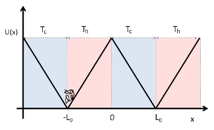
Figure 1: (Color online) Schematic diagram for initially coiled polymer chain in a piecewise linear bistable potential in the absence of an external load. The potential wells and the barrier top are located at $x=\pm L_{0}$ and $x=0$, respectively. Due to the thermal background kicks, the polymer ultimately attains a steady state velocity as long as there is a distinct temperature difference between the hot and cold reservoirs.

II The model

We consider a flexible polymer chain of size $N$ which undergoes a Brownian motion in a one dimensional piecewise linear bistable potential with an external load $U(x)=U_{s}(x)+fx$ where the ratchet potential $U_{s}(x)$ is described by

$$U_{s}(x)=\cases{U_{0}\left({x\over L_{0}}+1\right),&if $-L_{0}\leq x\leq 0$;\cr U_{0}\left({-x\over L_{0}}+1\right),&if $0\leq x\leq L_{0}.$\cr}$$ (1)

Here, $U_{0}$ and $2L_{0}$ denote the barrier height and the width of the ratchet potential, respectively, and where $f$ is the load. The potential has a potential maxima $U_{0}$ at $x=0$ and potential minima at $x=\pm L_{0}$. In this work, the chain contour length is taken to be much less than the characteristic dimension of the ratchet potential $2L_{0}$. The ratchet potential is also coupled with a spatially varying temperature

$$T(x)=\cases{T_{h},&if $-L_{0}\leq x\leq 0$;\cr T_{c},&if $0\leq x\leq L_{0}$\cr}$$ (2)

as shown in Fig. 1. $U_{s}(x)$ and $T(x)$ are assumed to have the same period such that $U_{s}(x+2L_{0})=U_{s}(x)$ and $T(x+2L_{0})=T(x)$.

Considering only nearest-neighbor interaction between the polymer segments (the bead spring model), the Langevin equation that governs the dynamics of the $N$ beads $(n=1,2,3,...,N)$ in a highly viscous medium under the influence of external potential $U(x)$ is given by

$$\gamma{dx_{n}\over dt} = -k(2x_{n}-x_{n-1}-x_{n+1})-{\partial U(x_{n})\over\partial x_{n}}+$$

$$\sqrt{2k_{B}\gamma T(x_{n})}\xi_{n}(t)$$

where the $k$ is the spring (elastic) constant of the chain while $\gamma$ denotes the friction coefficient. $\xi_{n}(t)$ is assumed to be Gaussian white noise and $k_{B}$ denotes the Boltzmann constant. Hereafter, we assume $k_{B}$ to be unity.

To simplify model equations we introduce a dimensionless load ${\bar{f}}=fL_{0}/T_{c}$, rescaled temperature ${\bar{T}}(x)=T(x)/T_{c}$, rescaled barrier height ${\bar{U}_{0}}=U_{0}/T_{c}$ and rescaled length ${\bar{x}}=x/L_{0}$. We also introduced a dimensionless coupling strength ${\bar{k}}=kL_{0}^{2}/T_{c}$, $\tau=T_{h}/T_{c}$ and time ${\bar{t}}=t/\beta$ where $\beta=\gamma L_{0}^{2}/T_{c}$ denotes the relaxation time. From now on, $\beta$ and $\gamma$ are taken to be unity and all the quantities are rescaled (dimensionless) so that the bars will be dropped.

III Flexible polymer chain

Previous studies have shown that a single monomer (a Brownian particle) attains a directional motion when it is exposed to a ratchet potential coupled with a spatially variable temperature or an external load. For such a system, the functional dependence for the steady state current $J$ or the velocity $V$ on the system parameters is well explored m1 ; m2 ; m3 . However, it is not known how these results apply to a chain with several monomers. Here, we will explore the dependence of the unidirectional chain velocity as a function of key system parameters.

Next in order to understand how the velocity of the chain responds to the change to its conformational flexibility and variability that arise due to its internal degree of freedoms, we simulate the Brownian dynamics given by Eq. (3) and compute the steady state current. This result is then averaged over $10^{4}$ independent simulations.

To analyze further how the polymer or in general any linearly coupled system responds to the nonhomogeneous thermal noise while surmounting a double-well potential with load, the dependence of the velocity as a function of the different system parameters is explored. The numerical and analytical analyses reveal that the polymer exhibits a unidirectional current where the strength of the current rectification relies not only on the thermal background kicks and load but it has also a nontrivial dependence on its coupling strength and size. It is found that in the absence load $f=0$, the chain maintains a positive current as long as a distinct temperature difference between the hot and cold reservoirs is retained; i.e, $T_{h}>T_{c}$, $V>0$. For isothermal case, a one dimensional negative current can be achieved providing $f\neq 0$. In general when $T_{h}>T_{c}$ and $f\neq 0$, the polymer exhibits intriguing transport features. Figures 2 plots the velocity $V$ as a function of $k$ for fixed external load $f=0.0$ and $f=4.0$, respectively. The numerical results exhibits that in the limit $k\to\infty$, $V$ goes to the velocity of a rigidly coupled polymer (dashed blue line) that evaluated via Eq. (8); when $k\to 0$, $V$ approaches to the velocity of a single Brownian particle ( dashed blue line) that evaluated using Eq. (8). The same figure depicts that the chain retains a higher velocity at $k=0$ than a globular chain ($k\to\infty$). Another crucial feature such model system is that the chain internal degree of freedoms has the capacity to enhance the chainӳ speed. As a result, the current does manifest a noticeable optimal peak at a certain optimal $k$.

Figure 2: (Color online) The velocity $V$ as a function of $k$ for parameter choice $f=0.0$ (red solid line) and $f=4.0$ ( black solid line). In the figure, other parameters are fixed as $N=2.0$, $U_{0}=6.0$ and $\tau=2.0$. The dashed blue lines are from the exact analytic results (Eq. (8)) both in the limit of $k\to\infty$ and $k\to 0$

Next via numerical simulations, we explore the dependence of the chain stall force $f^{\prime}$ on its internal degree of freedoms. Surprisingly the numerical analysis reveals that for the flexible polymers with finite $k$, the stall force is still independent of $N$ which is in agreement to the exact analytical result for the globular chain (see Eq. (9)). At this point we want to stress that the external load dictates the direction of the particle flow. When $f<f^{\prime}$, the net current is positive and while on the contrary for $f>f^{\prime}$, the current flows from the cold to the hot reservoirs. It worth noting that a larger polymer moves sluggishly than a smaller chain as long as $f\neq f^{\prime}$. At stall force $f=f^{\prime}$, the polymer will have zero velocity regardless its size. In Fig. 3a, we plot $V$ as a function of $f$. In the figure, the green solid lines stand the plot for $V$ in the limit of $k\to 0$ (top) and $k\to\infty$. The dotted lines are analyzed from the simulations for given values of $k=0$, $k=8.0$ and $k=25.0$ (globular chain) from the top to bottom, respectively. As depicted in Fig. 3a, for polymer with finite $k$, current reversal occurs at $f=2.0$ for parameter choice $U_{0}=6.0$ and $\tau=2.0$ regardless of the magnitude of $k$ revealing that the coupling strength is not a relevant control parameter to alter the direction of polymer s current. On the other hand Figure 3b depicts the plot of $V$ as a function of $U_{0}$ for a parameter choice $f=0.3$ and $\tau=2.0$. As shown in the figure, the velocity for the polymer monotonously increases with $U_{0}$ and attains a maximum value at a particular optimum barrier height $U_{0}^{opt}$. Further increasing in $U_{0}$ leads to a smaller $V$. At $U_{0}^{opt}$, the chain retains a maximum speed. The same figure shows that the velocity increases when $k$ decreases. $U_{0}^{opt}$ also strictly relies on $k$; when $k$ decreases, $U_{0}^{opt}$ increases. Furthermore, our analysis exhibits that the transport property of the chain also strictly relies on the temperature difference between the hot and cold baths. When the magnitude of the rescaled temperature $\tau$ steps up, the tendency for the polymer in the hot bath to reach the top of the ratchet potential increases than the chain in the cold reservoir. This leads to an increase in the current or velocity.

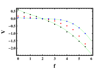
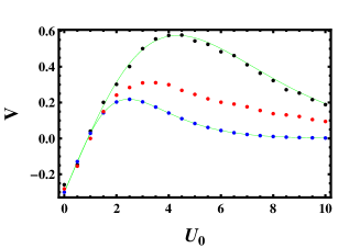
Figure 3: (Color online)(a) The velocity $V$ as a function of $f$ for the parameter values of $U_{0}=6.0$, and $\tau=2.0$. The green solid lines stand the plot for $V$ in the limit of $k\to 0$ (top) and $k\to\infty$. The dotted lines are analyzed from the simulations for given values of $k=0$, $k=8.0$ and $k=25.0$ (globular chain) from the top to bottom, respectively. (b) The velocity $V$ as a function of $U_{0}$ for parameter choice $k=0$, $k=5.0$ and $k=25.0$ ( compact chain), from top to bottom. We also fixed $f=0.3$ and $\tau=2.0$; dotted line stands for the simulation results while green solid lines are form analytic prediction.

Figure 4: (Color online) The velocity $V$ as a function of $N$ for parameter choice $f=0$ and $f=2.0$ from top to bottom. In the figure, other parameters are fixed as $k=20$, $U_{0}=4.0$ and $\tau=2.0$.

The dependence of the velocity on chain s length is also investigated for parameter choice $f=0$ and $f=2.0$ from top to bottom. In the figure, other parameters are fixed as $k=20$, $U_{0}=4.0$ and $\tau=2.0$. (see Fig. 4). The figure depicts that when the load is not strong enough, the polymer attains a positive current while for large load, the system exhibits a current reversal. In both cases, the chain velocity monotonously decreases as the chain length decreases.

IV Globular polymer chain

In order gain a deeper insight into this finding, it is instructive to compute the velocity for globular polymer as well as a single Browinian. In order to rewrite the Langevin equation for compact polymer or rigid polymer ($k\to\infty$) in terms of the center of mass motion, let us add the $N$ Langevin equations (Eq. (3)) to get

$${d\over dt}{(\sum_{i=1}^{N}x_{i})}=-\sum_{i=1}^{N}{\partial U(x_{i})\over\partial x_{i}}+\sum_{i=1}^{N}\sqrt{2\gamma T(x_{i})}\xi_{i}(t).$$ (4)

When a compact polymer of size $N$ hops on the ratchet potential, each monomer experiences the same force along the reaction coordinate. Hence the effective Langevin equation for the center of mass motion $x_{cm}=(x_{1}+x_{2}+...x_{N})/N$ can be written as

$$N{dx_{cm}\over dt}=-N{\partial U(x_{cm})\over\partial x_{cm}}+\sqrt{2\gamma T(x)}(\xi_{1}(t)+...+\xi_{N}(t)).$$ (5)

From fluctuation-dissipation relation

$$\left\langle(\xi_{1}(t)+...+\xi_{N}(t))(\xi_{1}(t)+...+\xi_{N}(t))\right\rangle=N\left\langle\xi(t)^{2}\right\rangle$$ (6)

which implies that we can substitute $(\xi_{1}(t)+...+\xi_{N}(t))$ by $\sqrt{N}\xi(t)$. After some algebra Eq. (5) converges to

$${dx_{cm}\over dt}=-{\partial U(x_{cm})\over\partial x_{cm}}+\sqrt{2\gamma T_{cm}(x)}\xi(t)/\sqrt{N}.$$ (7)

The corresponding steady state current $J$ can be exactly evaluated using the same approach as the work m3 . After some algebra, we find a closed form expression for the steady state current

$$J=-{\varsigma_{1}\over\varsigma_{2}\varsigma_{3}+\varsigma_{4}\varsigma_{1}}$$ (8)

where the expressions for $\varsigma_{1}$, $\varsigma_{2}$, $\varsigma_{3}$ and $\varsigma_{4}$ are given as $\varsigma_{1}=e^{a-b}-1$, $\varsigma_{2}={N\over a\tau}\left(1-e^{-a}\right)+{N\over b}e^{-a}\left(e^{b}-1\right)$, $\varsigma_{3}={1\over a}\left(e^{a}-1\right)+{1\over b}e^{a}\left(1-e^{-b}\right)$. The parameter $\varsigma_{4}$ is given by $\varsigma_{4}=\epsilon_{1}+\epsilon_{2}+\epsilon_{3}$ where $\epsilon_{1}={N\over\tau}\left({1\over a}\right)^{2}\left(a+e^{-a}-1\right)$, $\epsilon_{2}={N\over ab}\left(1-e^{-a}\right)\left(e^{b}-1\right)$, $\epsilon_{3}=N\left({1\over b}\right)^{2}\left(e^{b}-1-b\right)$. Here $a=N\left(U_{0}+f\right)/\tau$ and $b=N\left(U_{0}-f\right)$. The corresponding velocity is given by $V=2J$. In the limit $f\gg U_{0}$ and large $N$ we have $a\approx Nf/\tau$, $b\approx-Nf$, $\varsigma_{1}\approx\exp[Nf/\tau+Nf]$, $\varsigma_{2}\approx 1/f$, $\varsigma_{3}\approx\exp[(Nf/\tau+Nf)]/Nf$, $\epsilon_{1}\approx 1/f$, $\epsilon_{2}\approx 0$ and $\epsilon_{3}\approx 1/f$. Substituting these values, we get $J\approx-f/2.$ Furthmore, the exact analytical result for the globular chain uncovers that the stall force

$$f^{\prime}={U_{0}(\tau-1)\over(\tau+1)}$$ (9)

at which the chain current vanishes, is independent of the chain length $N$.

In the absence of external load $f=0$, the steady state current (Eq.(8)) converges to

$$J={NU_{0}^{2}\over 2(1+\tau)}\left[{1\over e^{NU_{0}\over\tau}-1}-{1\over e^{NU_{0}}-1}\right].$$ (10)

For small $U_{0}$, it is straight forward to show $J\approx{U_{0}\over 2}\left({\tau-1\over\tau+1}\right).$ On the other hand for large $U_{0}$ and $\tau$, one approximates Eq. (10) as $J\approx{NU_{0}^{2}\over 2(1+\tau)}e^{-NU_{0}\over\tau}.$

Closer look at the Fig. 2 once again reveals that the chain retains a higher velocity $V(0)$ at $k=0$ than the velocity $V(\infty)$ of a globular chain ($k\to\infty$). Particularly, as the size of the chain increases, the gap between $V(0)$ and $V(\infty)$ increases. To analyze the chain size dependence further, we have computed the ratio for the velocity of a single particle to globular polymer utilizing Eq. (8). As exhibited in Fig. 5, $V$ is a nontrivial function of $N$; the polymer with small $k$ retains considerably higher velocity than a rigid dimer. This signifies that attenuating the strength of the elastic constant results in a polymer that can be transported fast. This can be notably appreciated by taking the velocity ratio between a single and globular polymer in high barrier limit which is given as

$${V(0)\over V(\infty)}={e^{(-1+N)(fL_{0}+U_{0})\over\tau}\over N}$$ (11)

where in the limit $f\to 0$, ${V(0)\over V(\infty)}={\exp^{(-1+N)(U_{0})\over\tau}\over N}$. This can be retrieved using our previous calcualtions since for large $U_{0}$, $J\approx{NU_{0}^{2}\over 2(1+\tau)}e^{-NU_{0}\over\tau}.$

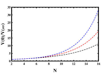
Figure 5: The ratio $V(k\to 0)/V(k\to\infty)$ as a function of $N$ for parameter choice $f=0.0$ (black solid line), $f=0.5$ (red solid line), $f=1.0$ (blue solid line). Other parameters are fixed as $U_{0}=2.0$ and $\tau=8.0$.

The central results of this paper also indicates the occurrence a direct relationship between the flexibility of a macromolecule and its transport properties. Hence, we expect that in general this relationship can be applied to control the transport of molecules by modulating their flexibility. Modifying the flexibility of a macromolecule can be achieved in a variety of ways. Experimentally, the flexibility of the chain can be manipulated in a variety of ways. For instance, the flexibility of proteins can be altered by ligand binding m10 . The elasticity of the DNA molecule can be also strengthen by introducing external charges m11 . Thermal and chemical denaturation also alter the flexibility of biological molecules since hydrogen bond breaking leads to an increase in the rotational degrees of freedom of atoms and thereby increases the macroscopic flexibility of the molecule m12 ; m122 .

V Summary and conclusion

We study the transport and response properties of a single flexible polymer moving in a ratchet potential with an external load where the viscous medium is alternately in contact with inhomogeneous temperature along the reaction coordinate. As long as the system is far from equilibrium, we show that each monomer of the chain exhibits a fast unidirectional current where the strength of the current rectification relies not only on the thermal background kicks and load but it has also a nontrivial dependence on its coupling strength and size.

The numerical and exact analyses indicate that the stall force is independent of the chain length $N$ and coupling strength $k$. It is also shown that a flexible chain retains a higher velocity than a less flexible polymer revealing that a chain with a desired speed can be fabricated by attenuating the strength of the elastic constant. The chain s flexibility can be modified through ligand binding m10 , by introducing external charges m11 and via chemical denaturation m12 ; m122 .

In conclusion, in this work, we present a pragmatic model system which not only serves as a basic guide on how to transport the polymer fast to specific region but also has novel applications for binding kinetics, DNA amplifications and sorting of multicomponent systems based on their dominant parameters

Acknowledgment.— This work was supported in part by the National Heart, Lung, and Blood Institute (Grant No. R01HL101196). I would like to thank Yohannes Shiferaw for the interesting discussion I had. I would like also to thank Mulu Zebene for the constant support.

References

- (1) P. Hänggi, P. Talkner and M. Borkovec, Rev. Mod. Phys. 62, 251 (1990).
- (2) K. L. Sebastian and A. Debnath, J. Phys. Condens. Matter 18, S283 (2006).
- (3) P. J. Park and W. Sung, J. Chem. Phys. 111, 5259 (1999).
- (4) S. Lee and W. Sung, Phys. Rev. E 63, 021115 (2001).
- (5) F. Marchesoni, C. Cattuto and G. Costantini, Phys. Rev. B 57, 7930 (1998).
- (6) K. L. Sebastian and A. K. R. Paul, Phys. Rev. E 62, 927 (2000).
- (7) J. F. Lindner, B. K. Meadows, W. L. Ditto, M. E. Inchiosa, and A. R. Bulsara, Phys. Rev. Lett. 75, 3 (1995); Phys. Rev. E 53, 2081 (1996).
- (8) F. Marchesoni, L. Gammaitoni, and A. R. Bulsara, Phys. Rev. Lett. 76, 2609 (1996).
- (9) I. E. Dikshtein, D. V. Kuznetsov and L. S. Geier, Phys. Rev. E. 65, 061101 (1996).
- (10) M. Asfaw and W. Sung, EPL 90, 3008 (2010).
- (11) M. Asfaw, Phys. Rev. E 82, 021111 (2010).
- (12) M. Asfaw and Y. Shiferaw, J. Chem. Phys. 136, 025101 (2012).
- (13) P. Jung, U. Behn, E. Pantazelou, and F. Moss, Phys. Rev. A 46, R1709 (1992).
- (14) A. Pototsky, F. Marchesoni, and S. E. Savel’ev, Phys. Rev. E 81, 031114 (2010).
- (15) A. Pototsky, N. B. Janson, F. Marchesoni, S. E. Savel’ev, Chem. Phys. 375, 458 (2010).
- (16) E. Heinsalu, M. Patriarca, and F. Marchesoni, Phys. Rev. E 77, 021129 (2008).
- (17) O. M. Braun, R. Ferrando and G. E. Tommei, Phys. Rev. E 68, 051101 (2003).
- (18) C. Fusco, A. Fasolino and T. Janssen, Eur. Phys. J. B 31, 95 (2003).
- (19) P. S. Burada, G. Schmid, D. Reguera, M. H. Vainstein, J. M. Rubi, and P. Hänggi, Phys. Rev. Lett. 101, 130602 (2008).
- (20) R. Benzi, G. Parisi, A. Sutera and A. Vulpiani, Tellus 34, 10 (1982).
- (21) L. Gammaitoni, P. Hänggi, P. Jung and F. Marchesoni, Rev. Mod. Phys. 70, 223 (1998).
- (22) S. Klumpp, A. Mielke and C. Wald, Phys. Rev. E 63, 031914 (2000).
- (23) M. T. Downton, M. J. Zuckermann, E. M. Craig, M. Plischke and H. Linke, Phys. Rev. E 73, 011909 (2006).
- (24) J. M. Polson, B. Bylhouwer, M. J. Zuckermann, A. J. Horton, and W. M. Scott, Phys. Rev. E 82, 051931 (2010).
- (25) J. Rousselet, L. Salome, A. Ajdari and J. Prost, Nature 370, 446 (1994).
- (26) L. P. Faucheux, L. S. Bourdieu, P. D. Kaplan and A. J. Libchaber, Phys. Rev. Lett. 74, 1504 (1995).
- (27) L. Gorre, E. Ioannidis and P. Silberzan, Europhys. Lett. 33, 267 (1996).
- (28) L. G. Talini, J. P. Spatz and P. Silberzan, Chaos 8, 650 (1998).
- (29) G. W Slater, H. L. Guo, and G. I. Nixon, Phys. Rev. Lett. 78, 1170 (1997).
- (30) J. Bader, R. W. Hammond, S. A. Henck, M. W. Deem, G. A. McDermott, J. M. Bustillo, J. W. Simpson, G. T. Mulhern, and J. M. Rothberg, Proc. Natl. Acad. Sci. U.S.A. 96, 13165 (1999).
- (31) M. Büttiker, Z. Phys. B 68, 161 (1987).
- (32) N. G. Van Kampen, IBM J. Res. Dev. 32, 107 (1988).
- (33) M. Asfaw and M. Bekele, Eur. Phys. J. B 38, 457 (2004).
- (34) M. Asfaw, Eur. Phys. J. B 65, 109 (2008).
- (35) R. Landauer, J. Stat. Phys. 53, 233 (1988).
- (36) R. Landauer, Phys. Rev. A 12, 636 (1975).
- (37) R. Landauer, Helv. Phys. Acta 56, 847 (1983).
- (38) M. Matsuo and Shin-ichi Sasa, Physica A 276, 188 (1999).
- (39) F. Jülicher, A. Ajdari and J. Prost, Rev. Mod. Phys. 69, 1269 (1997).
- (40) R. L. Najmanovich, J. Kuttner, V. Sobolev, and M. Edelman, Proteins: Struct., Funct., Genet. 39, 261 (2000).
- (41) A. Podest, M. Indrieri, D. Brogioli, G. S. Manning, P. Milani, R. Guerra, L. Finzi, and D. Dunlap, Biophys. J. 89, 2558 (2005).
- (42) B. Schulze, A. Sljoka, and W. Whiteley, AIP Conf. Proc. 1368, 135 (2011).
- (43) B. M. Hespenheid, A. J. Rader, M. F. Thorpe, and L. A. Kuhn, J. Mol. Graphics Model. 21, 195 (2002).