Distributed Monitoring for Prevention of Cascading Failures in Operational Power Grids

Abstract

Electrical power grids are vulnerable to cascading failures that can lead to large blackouts. Detection and prevention of cascading failures in power grids is important. Currently, grid operators mainly monitor the state (loading level) of individual components in power grids. The complex architecture of power grids, with many interdependencies, makes it difficult to aggregate data provided by local components in a timely manner and meaningful way: monitoring the resilience with respect to cascading failures of an operational power grid is a challenge.

This paper addresses this challenge. The main ideas behind the paper are that (i) a robustness metric based on both the topology and the operative state of the power grid can be used to quantify power grid robustness and (ii) a new proposed a distributed computation method with self-stabilizing properties can be used to achieving near real-time monitoring of the robustness of the power grid. Our contributions thus provide insight into the resilience with respect to cascading failures of a dynamic operational power grid at runtime, in a scalable and robust way. Computations are pushed into the network, making the results available at each node, allowing automated distributed control mechanisms to be implemented on top.

1 Introduction

Power grids represent critical infrastructure: all kind of services (basic services, governmental and private) depend on the continuous and reliable delivery of electricity. Power grid outages have a large effect on society, both in terms of safety and in terms of economic loss. The large-scale introduction of “renewable energy sources” and the current (centralized) architecture of the power grid make it more likely that large power outages will become more common. Encouraged by government subsidies and a trend to become more “green”, consumers are becoming producers of electricity by installing solar panels and wind mills [26]. Part of this produced power will be used locally, but excess power can be sold and fed back into the power grid. This in turn leads to grid instability [40]: it is more difficult to predict, and hence balance, electricity production when there is a large amount of small producers spread over a large geographical region, instead of a couple of large producers. The current power grid architecture does not support the introduction of renewables at this scale [1].

The current organization of the power grid thus makes larger grid failures more likely to occur: initial local disruptions can spread to the rest of a power grid evolving into a system-wide outage. In a power grid, an initial failure can, for example, be caused by an external event such as a storm, and spreads to the rest of the network in different ways including due to causes such as instability of voltage and frequency, hidden failures of protection systems, software or operator errors, and line overloads. For example, in the case of cascades due to line overloads, an overloaded line is "tripped” by a circuit breaker. At this point electricity can no longer flow through the line, and the power contained in the line flows to other lines. This might lead to overloading (part of) these lines causing them to be tripped as well. As this process repeats over and over again, more lines are shut down, leading to a cascading failure of the power grid [12, 33]. Cascading effect due to line overloads, and preventing such cascading failures form the main focus of this paper.

In order to detect (and ultimately prevent) cascading failures it is necessary to monitor (and alter) the current state (power load distribution) of the power grid. The emerging Smart Grid provides exactly this: a power grid with a communication overlay that connects sensors and effectors. In effect, a Smart Grid is a large-scale distributed system that enables the monitoring of line loads and that enables changing the state of the network by tripping and untripping lines. In the remainder of the paper a Smart Grid is assumed.

Given this context of the Smart Grid, this paper addresses two main research questions: What should be monitored?, i.e., is there a metric that can be used for cascading failure prediction? How to monitor?, i.e., how should aggregation be performed and which temporal resolution is required for the monitoring. In addition, it should be possible to extend the proposed (passive) monitoring scheme to an (active) scheme that automatically alters the state of the grid in order to prevent cascading failures.

The main contribution of the paper is a new distributed monitoring approach that can be used to monitor the robustness of the power grid with respect to cascading failures. The monitoring approach is based on the distributed computation of the robustness metric we introduced in [23, 24]. Our contributions in this paper include the extension of a distributed gossiping algorithm [9] with self-stabilization mechanisms to account for network dynamics. The resulting framework allows distributed aggregates to be computed fast and reliable, which forms the core of the proposed monitoring approach.

Our main results show that we are able to compute the complex robustness metric using simple robust distributed primitives with results readily made available at each node in the network. This is an important property as the mechanisms presented in this paper can be seen as a measurement framework to be used in real-time for the design of distributed control mechanisms. Our approach scales very well with network size (logarithmic order) in terms of convergence time. The precision of the computations can be fixed by changing the message sizes and is independent on the network parameters (number of nodes, diameter, etc.).

The remainder of this paper is organized as follows: Section 2 introduces the metric used to assess the robustness of the power grid with respect to cascading failures. Section 3 presents the distributed algorithm for the online computation of the robustness metric. Section 4 discusses the simulation results that show the applicability the proposed approach. Section 5 presents the current state of the art in power grid monitoring and cascading failure detection. Section 6 concludes the paper.

2 Robustness Metric

Different topological metrics have been identified in literature that indicate the vulnerability of a power grid against cascading failures on the basis of which the most critical nodes in a network are identified. Examples of such topological metrics are average shortest path length, betweenness centrality [15] and the gap metric [13]. However, next to a topological aspect, power grids also have a physical aspect. In particular, electrical current in a power grid behaves according to Kirchoff’s laws [5]. A metric that quantifies the robustness of an operational power grid with respect to cascading failures should take both these aspects into account. Our robustness metric from [23, 24] does exactly this, and it therefore forms the starting point for the distributed power grid monitoring algorithm proposed in this paper. The robustness metric $R_{CF}$ (for Robust against Cascading Failures) assess the robustness of a given power grid with respect to cascading failures due to line overloads. The metric relies on two main concepts: electrical nodal robustness and electrical node significance. Higher values of $R_{CF}$ indicate a robuster, i.e., more able to resist cascading failures, power grid. The remainder of this section provides a summary from our earlier work on robustness metrics, we refer to [23, 24] for more details.

2.1 Electrical Nodal Robustness

The electrical nodal robustness quantifies the ability of a bus (i.e. a node in a graph representation of a power grid) to resist the cascade of line overload failures by incorporating both flow dynamics and network topology. In order to calculate this value for a node, three factors are of importance: (i) the homogeneity of the load distribution on out-going branches (i.e. links in a graph representation of a power grid); (ii) the loading level of the out-going links; and (iii) the out-degree of the node.

Entropy is used to capture the first and the last factors described above: the entropy of a load distribution at a node increases as flows over lines are distributed more homogeneously and the node out-degree increases. The entropy of a given load distribution at a node $i$ is computed by Equation (1):

$$H_{i}=\sum_{j=1}^{d}p_{ij}\log p_{ij}$$ (1)

where $d$ refers to the out-degree of the corresponding node, whereas $p_{ij}$ corresponds to normalized flow values on the out-going links $l_{ij}$, given as:

$$p_{ij}=\frac{f_{ij}}{\sum_{j=1}^{d}f_{ij}}$$ (2)

where $f_{ij}$ refers to the flow value in line $l_{ij}$. To model the effect of the loading level of the power grid the tolerance parameter $\alpha$ is used (see [30]). The tolerance level of a line $l_{ij}$, $\alpha_{ij}$, is the ratio between the rated limit and the load of the corresponding line $l_{ij}$.

Combining Equations (1) and (2) with the tolerance parameter $\alpha$ to capture the impact of loading level on the robustness, the electrical nodal robustness of a node $i$ (i.e. $R_{n,i}$), which takes both the flow dynamics and topology effects on network robustness into account, is then defined as:

$$R_{n,i}=-\sum_{j=1}^{d}\alpha_{ij}p_{ij}\log p_{ij}$$ (3)

In Equation (3), the minus sign (-) is used to compensate the negative electrical nodal robustness value that occurs due to taking the logarithm of normalized flow values.

2.2 Electrical Node Significance

Not all nodes in a power grid have the same influence on the occurrence of cascading failures. Some nodes distribute a relatively large amount of the power in the network, while other nodes only distribute a small amount of power. When a node (or line to a node) that distributes a relatively large amount of power fails, the result is more likely to lead to a cascading failure, ultimately resulting in a large grid blackout. In contrast, if a node that only distributes a small amount of power fails, the resulting redistribution of power can usually be accommodated by the other parts of the network. Thus, node failures have a different impact on the context of cascading failure robustness and this impact depends on the amount of power, distributed by the corresponding node. The impact of a particular node is reflected by the electrical node significance $\delta$, which is:

$$\delta_{i}=\frac{P_{i}}{\sum_{j=1}^{N}P_{j}},$$ (4)

where $P_{i}$ stands for total power distributed by node $i$ while, $N$ refers to number of nodes in the network. Electrical node significance is a centrality measure that can be used to rank the relative importance (i.e., criticality) of nodes in a power grid in the context of cascading failures. Failures of nodes with a higher $\delta$ will typically result in larger cascading failures.

2.3 Network Robustness Metric

The network robustness metric $R_{CF}$ ([23, 24]) is obtained by combining the nodal robustness and node significance:

$$R_{CF}=\sum_{i=1}^{N}R_{n,i}\delta_{i}.$$ (5)

The above metric can be used as a robustness indicator for power grids. This is done as follows: for a normally operating power grid the robustness metric is calculated, which results in some value $v$. This value is used as a base case. During normal operation the robustness metric value will change somewhat, because different nodes will demand different electricity quantities over time, leading to different loading levels in the network. However, a larger change in the robustness metric, a drop in particular, indicates that a cascading failure becomes more likely and grid operators may need to take evasive actions (e.g., adding reserve capacity to the grid or demand shifting of power). Note that, in the general case, it is complicated to determine what good safety margins are, or for which values of the robustness metric the exact tipping point is located (i.e., the point where a small failure will lead to a massive blackout). Ultimately this needs to be determined by the grid operators. We have determined this point experimentally, by simulation, for a specific power grid: the IEEE 118 Power system (see Section 4.4 ). We refer to [25] which presents a more general and structured investigation of this topic.

3 Decentralized Aggregation

The computation of the robustness metric introduced in the previous section in a centralized manner raises a number of challenges when applied to large areas (i.e., provinces or even whole countries). Scalability, single-point-of-failure, real-time results dissemination, fault tolerance, maintenance of dedicated hardware are just a few examples that hint towards a decentralized approach as a more convenient solution.

The described problem maps onto a geometric random graph (mesh network), where the nodes can communicate mainly with their direct neighbors. From the perspective of the communication model, we assume that time is discrete. During one time step each node will pick and communicate with a random neighbor. Major updates in the network occur just once in a while (for example, in the described scenario, new measurement data is made available once every 15 minutes). We will make use of the concept of time rounds and ask the nodes to update their local data at the beginning of the rounds. The bootstrap problem and round-based time models received a lot of attention in literature [19, 6, 31] - in our application scenario the constraints being very loose allow for an algorithm like the one presented in [35].

We make no assumptions with respect to nodes stop-failing or new nodes joining the network. The mechanism described below can accommodate these cases and the computation results will adapt themselves to such changes.

3.1 Solution Outline

Our solution for computing the robustness metric uses a primitive for computing sums in a distributed network inspired by the gossip-alike mechanism presented in [28] (see Figure 1). The algorithm presented in [28] computes a sum of values distributed on the nodes of a network by using a property of order statistics applied to a series of exponential random variables. The algorithm resembles gossiping algorithms [19] but differs in a number of important points.

Essentially, it trades communication for convergence speed. By relying on the propagation of an extreme value (the minimum value in this case), locally computable, it achieves the fastest possible convergence in a distributed network - $O(D\log N)$ time steps ($D$ is the diameter of the network and $N$ the number of nodes). This speed is significant compared to the original gossiping algorithms that converged in $O(D^{2}\log N)$ time steps [9]. For example, in Figure 1 a $N=1000$ nodes network with diameter $14$ converges after the first $15$ computation steps. The paid price is the increased messages size $O(\delta^{-2})$, where $\delta$ is a parameter defining the precision of the final result. Assuming $s$ as the ground-truth result, the algorithm offers an estimate in the interval $[(1-\delta)s,(1+\delta)s]$ with an error $\epsilon=O(1/poly(N))$.

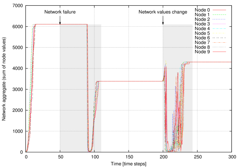
Figure 1: Sum computation during network dynamics (geometric random graph with $1000$ nodes initially, diameter 14, random values, half of the network is disconnected at time 50, nodes change their values at at time 200).

We extend the extreme value propagation mechanisms to account for dynamics in the network. Specifically, we add a time-to-live field to each value - an integer value that decreases with time and marks the age of the current value. This mechanism takes care of nodes leaving the network, stop-crashing or resetting. In the example in Figure 1, after convergence, we removed half of the nodes in the network at time $50$. The effect of expiring time-to-live (set to a maximum of $50$ in this example) can be seen around the time step $100$. Furthermore, we extend the time-to-live expiry mechanism to achieve a $O(D\log N+\log T)$ time steps value removal. In other words, if a certain extreme value propagated through the network, we mark it as “expired” and assure its associated time-to-live value to expire (reach 0) within $O(D\log N+\log T)$ time steps. This is shown in Figure 1 in the interval $200-300$. At time $200$ half of the nodes in the network changed their values randomly triggering the expiration mechanism.

Our distributed approach solves most of the scaling issues and proves to be highly robust against network dynamics (e.g., network nodes becoming unavailable due to failures, reconfiguration, new nodes joining the system, etc.). As we show in the following, our approach is very fast for a typical network, outperforming by far the speed of centralized approaches. As the protocols rely on anonymous data exchanges, privacy issues [27] are alleviated, as the identities of the system participants are not needed in the computations.

The downsides of our approach map onto the known properties of this class of epidemic algorithms. Although anonymity is preserved, an authentication system [20] is needed to prevent malicious data corrupting the computations. Also, a light form of synchronization [35] is needed for coordinating nodes to report major changes in their local values - fortunately, the nature of the problem we address here allows it.

3.2 Self-stabilizing Sum Computation - $ComputeSum()$

The basic mechanism behind the sum computation algorithm presented below relies on minimum value propagation via gossiping. Assume that each node holds a positive value $x_{i}$. At each time step, each node chooses a random neighbor and they exchange their values, both keeping the smallest value. The smallest value propagates fast in the network, in $O(D\log N)$ time steps, via this push-pull gossiping mechanism (see [32] Section 3.2.2.4 page 32).

1

2 /* $v$, $\tau$ - received value and time-to-live */

3

4 /* $v_{local}$, $\tau_{local}$ - local value and time-to-live */

5

6 /* create temporary variables */

7 $(v_{m},v_{M})\leftarrow\left(\min(v,v_{local}),\max(v,v_{local})\right)$

8 $(\tau_{m},\tau_{M})\leftarrow$ corresponding $(\tau,\tau_{local})$ to $(v_{m},v_{M})$

9

10 /* update logic */

11 if $v_{m}==v_{M}$ then

12       if $v_{m}<0$ then /* equal negative values */

13             $\tau_{m}\leftarrow\mathcal{C}\tau_{m}$

14      else  /* equal positive values */

15             $\min(\tau_{m},\tau_{M})\leftarrow\max(\tau_{m},\tau_{M})-1$

16else

17       if $v_{m}<0$ then /* at least one negative value */

18             if $v_{m}==-v_{M}$ then

19                   $(\tau_{m},\tau_{M})\leftarrow(T,T)$

20            else

21                   $(\tau_{m},\tau_{M})\leftarrow(\mathcal{C}\tau_{m},\mathcal{C}\tau_{M})$

22      else  /* two different positive values */

23             $\tau_{M}\leftarrow\tau_{m}-1$

24

25 /* update local variables */

26 $(v,v_{local})\leftarrow$ $(v_{m},v_{m})$

27 $(\tau,\tau_{local})\leftarrow$ corresponding $(\tau_{m},\tau_{M})$

ALGORITHM 1 PropagateMinVal($v,\tau$)

Assume that each node $i$ in the network holds a positive value $x_{i}$. In order to compute the sum of all $n$ values in the network $\left(\sum_{i=1}^{N}x_{i}\right)$, the authors of [28] propose that each node holds a vector $\mathbf{v}$ of $m$ values, initially drawn from a random exponential random distribution with parameter $\lambda_{i}=x_{i}$. After a gossiping step between two nodes $i$ and $j$, the vectors $\mathbf{v}_{i}$ and $\mathbf{v}_{j}$ become equal and hold the minimum value on each position of the initial vectors. Thus, given an index $k\in(1,m)$, the resulting vectors $\mathbf{v}^{\prime}_{i}$, $\mathbf{v}^{\prime}_{j}$ will have the property $\mathbf{v}^{\prime}_{i}[k]=\mathbf{v}^{\prime}_{j}[k]=\min\left(\mathbf{v}_{i}[k],\mathbf{v}_{j}[k]\right)$. The authors show that, after all vectors converge to some value $\mathbf{v}$, the sum of $x_{i}$ values in the network may be approximated by: $\sum_{i=1}^{N}x_{i}=\frac{m}{\sum_{k=1}^{m}\mathbf{v}[k]}$ (see [32] Section 5.2.5.4 page 75).

We extend the algorithm presented in [28] by adding to each node a new vector $\boldsymbol{\tau}_{i}$ holding a time-to-live counter for each value. This new vector is initialized with a default value $T$, larger than the convergence time of the original algorithm (choosing a proper value is explained below). The values in $\boldsymbol{\tau}_{i}$ decrease with $1$ every time slot, with one exception. The node generating the minimum $\mathbf{v}_{i}[k]$ on the position $k\in(1,m)$ sets $\boldsymbol{\tau}_{i}[k]$ to $T$ (see Algorithm 2 line 2). In the absence of any other dynamics, all properties proved in [32] remain unchanged as the output of our approach is identical to the original algorithm.

The main reason for adding the time-to-live field is to account for nodes leaving the network or nodes that fail-stop. We avoid this way complicated mechanisms in which nodes need to keep track of neighbors. Additionally, this mechanism does not make use of node identifiers. The intuition behind this mechanism is that a node generating the network-wide minimum on position $k\in(1,m)$ will always advertise it with the accompanying time-to-live set to the maximum $T$. The rest of the nodes will adopt the value $\mathbf{v}[k]$ and have a value $\boldsymbol{\tau}[k]$ decreasing with the distance from the original node. $T$ is chosen to be larger than the maximum number of gossiping steps it takes the minimum to reach any node in the network. In a gossiping step between two nodes $i$ and $j$, if $\mathbf{v}_{i}[k]=\mathbf{v}_{j}[k]$ then the largest of the $\boldsymbol{\tau}_{i}[k]$ and $\boldsymbol{\tau}_{j}[k]$ will propagate (Algorithm 1 line 1). This means that $\boldsymbol{\tau}[k]$ on all nodes will be strictly positive for as long as the node is online. If the node that generated the minimum value on the position $k$ goes offline, all the associated $\boldsymbol{\tau}[k]$ values in the network will steadily decrease (Algorithm 2 line 2) until they will reach $0$ and the minimum will be replaced by next smallest value in the network (Algorithm 2 lines 2-2). It will take $T$ time steps for the network to “forget” the value on position $k$. The graphical effect of this $O(T)$ mechanism is shown in Figure 1 in the interval $50-150$.

1

2 /* $\mathbf{v^{0}}$ - original random samples vector on this node */

3

4 /* $\mathbf{v},\boldsymbol{\tau}$ - received value and time-to-live vectors */

5

6 /* update all elements in the data vector */

7 for $j=1$ to length$(\mathbf{v})$ do

8       PropagateMinVal$(\mathbf{v}[j],\boldsymbol{\tau}[j])$

9

10 /* time-to-live update - do once every timeslot */

11 for $j=1$ to length$(\mathbf{v})$ do

12       if $\mathbf{v}[j]==\mathbf{v^{0}}[j]$ then /* reinforce a minimum */

13             $\boldsymbol{\tau}[j]\leftarrow T$

14      else

15             $\boldsymbol{\tau}[j]\leftarrow\boldsymbol{\tau}[j]-1$

16              /* decrease time-to-live */

17             if $\boldsymbol{\tau}[j]<=0$ then /* value expired */

18                   $\mathbf{v}[j]\leftarrow\mathbf{v^{0}}[j]$

19                   $\boldsymbol{\tau}[j]\leftarrow T$

20

21 /* estimate the sum of elements */

22 $s\leftarrow 0$

23 for $j=1$ to length$(\mathbf{v})$ do

24       $s\leftarrow s+abs(\mathbf{v}[j])$

return length$(\mathbf{v})/s$

ALGORITHM 2 ComputeSum $(\mathbf{v},\boldsymbol{\tau})$

The second self-stabilizing mechanism targets nodes changing their values at runtime. Assume a node changes its value $x_{i}$ to $x^{\prime}_{i}$ at some time $t$. This change will trigger a regeneration of its original samples from the exponential random variable $\mathbf{v}_{i}$ to $\mathbf{v}^{\prime}_{i}$. Let $k$ be an index with $k\in(1,m)$. Let $\mathbf{u}$ be the vector containing the minimum values in the network if the node $i$ would not exist. In order to understand the change happening when transitioning from $x_{i}$ to $x^{\prime}_{i}$ we need to look at the relationship between the individual values $\mathbf{v}_{i}[k]$, $\mathbf{v}^{\prime}_{i}[k]$ and $\mathbf{u}[k]$. As shown in Table 1, if $\mathbf{u}[k]$ is the smallest of all three values then no change will propagate in the network. If $\mathbf{v}^{\prime}_{i}[k]$ is the smallest value, then this will propagate fast, in $O(D\log N)$ time steps, with the basic extreme propagation mechanism. If $\mathbf{v}^{\prime}_{i}[k]$ is the smallest then this value will remain in the network until its associated time-to-live field will expire. As usually $T\gg D$ we add a mechanism to speed up the removal of this value from the network.

The removal mechanism is triggered by the node owning the value that needs to be removed (in our case node $i$) and works as follows: node $i$ will mark the value $\mathbf{v}_{i}[k]$ as “expired” by propagating a negative value $-\mathbf{v}_{i}[k]$. This change will not affect the extreme value propagation mechanism (see Algorithm 1) nor the estimation of the sum (notice the use of the absolute value function in Algorithm 2 line 2). If node $i$ contacts a node also holding the value $\mathbf{v}_{i}[k]$ then first, it will propagate the negative sign for the value, also maximizing its time-to-live field to a large value $T$. Intuitively, as long as the $\mathbf{v}_{i}[k]$ is present in the network, the $-\mathbf{v}_{i}[k]$ will propagate, over-writing it. Considering the large range of unique float or double numbers versus the number of values in a network at a given time, we can safely assume the values in the network to be unique.

The time-to-live field of any negative value will halve with each gossiping step (for $\mathcal{C}=2$) if it does not meet the $\mathbf{v}_{i}[k]$ value (Algorithm 1 lines 1, 1). Intuitively, if a negative value is surrounded by values other than $\mathbf{v}_{i}[k]$, it will propagate while canceling itself at the same time with an exponential rate. This mechanism resembles somewhat a predator-prey model [2], where prey is represented by the $\mathbf{v}_{i}[k]$ variable and predators by $-\mathbf{v}_{i}[k]$. We designed it such that the populations cancel each-others, targeting the fixed point at the origin as the solution for the accompanying Lotka-Volterra equations.

Propagation	Ordering	Previous	Intermediate	Final
none	$\mathbf{u}[k]<\mathbf{v}_{i}[k]<\mathbf{v}^{\prime}_{i}[k]$	$\mathbf{u}[k]$	$\mathbf{u}[k]$	$\mathbf{u}[k]$
	$\mathbf{u}[k]<\mathbf{v}^{\prime}_{i}[k]<\mathbf{v}_{i}[k]$	$\mathbf{u}[k]$	$\mathbf{u}[k]$	$\mathbf{u}[k]$
slow	$\mathbf{v}_{i}[k]<\mathbf{u}[k]<\mathbf{v}^{\prime}_{i}[k]$	$\mathbf{v}_{i}[k]$	$\mathbf{v}_{i}[k]$	$\mathbf{u}[k]$
	$\mathbf{v}_{i}[k]<\mathbf{v}^{\prime}_{i}[k]<\mathbf{u}[k]$	$\mathbf{v}_{i}[k]$	$\mathbf{v}_{i}[k]$	$\mathbf{v}^{\prime}_{i}[k]$
fast	$\mathbf{v}^{\prime}_{i}[k]<\mathbf{u}[k]<\mathbf{v}_{i}[k]$	$\mathbf{u}[k]$	$\mathbf{v}^{\prime}_{i}[k]$	$\mathbf{v}^{\prime}_{i}[k]$
	$\mathbf{v}^{\prime}_{i}[k]<\mathbf{v}_{i}[k]<\mathbf{u}[k]$	$\mathbf{v}_{i}[k]$	$\mathbf{v}^{\prime}_{i}[k]$	$\mathbf{v}^{\prime}_{i}[k]$

 

Table 1: Value propagation.

Lemma 3.1

Value removal delay

By using the value removal algorithm, the new minimum propagates in the network in $O(D\log N+\log T)$ time steps.

• In the worst case scenario, the whole network contains the minimum value $\mathbf{v}_{i}[k]$ on position $k$, with the time-to-live field setup at maximum $T$.The negative value, being the smallest one in the network, propagates in $O(D\log N)$ in the whole network. Again, in the worst case scenario, we will have a network with each node having the value $-\mathbf{v}_{i}[k]$ on position $k$ with the time-to-live set to the maximum $T$. From this moment on, the time-to-live will halve at each gossip step on each node (for $\mathcal{C}=2$), reaching $0$, in the worst case scenario in $O(\log T)$ time steps. This is the worst case because nodes may be contacted by several neighbors during a time step leading to a much faster cancellation. Overall, the removal mechanism will be active for at most $O(D\log N+\log T)$ time steps. This bound is an upper bound. In reality the spread and cancellation mechanisms will act in parallel, leading to tighter bounds.

This result gives us the basis for choosing the $T$ constant. Ideally, it should be chosen as small as possible, in line with the diameter of the network. The fact that the removal mechanism is affected only by $\log T$ lets us use an overestimate of $T$, which can be a few orders of magnitude larger than the diameter of the network, with little impact on the convergence speed. For example, if the network diameter is between $10-30$ and the values refresh each 10000 time steps, we can safely set $T$ anywhere between $1000-10000$ (see Section 4.3). This will not affect the convergence of the sum computation mechanism but allow for a timely account for a node removal.

All the mechanisms presented in this section lead to the sum computation mechanism $ComputeSum()$ presented in Algorithm 2. It holds the properties of the original algorithm described in [28] and it additionally showcases self-stabilization properties to account for network dynamics in the form of node removal and nodes changing their values in batches.

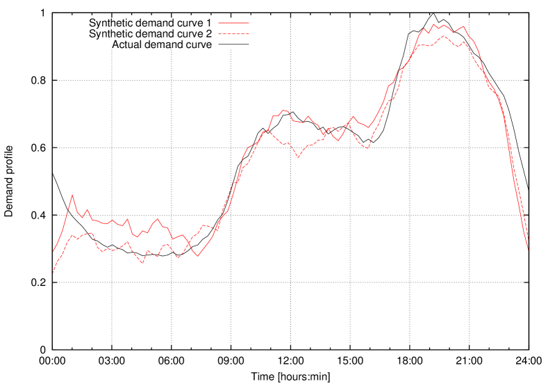
Figure 2: The actual demand profile from a point in Dutch transmission grid and two synthetically generated demand profiles.

3.3 Robustness Metric Computation

The robustness metric (see Section 2) is made up of two terms that can be computed locally ($p_{i}$ in Equation (2) and $R_{n,i}$ in Equation (3)) and two that can be computed in a distributed fashion ($\delta_{i}$ in Equation (4) and $R_{CF}$ in Equation (5)). Equation (5) can be rewritten as:

$$R_{CF} =\frac{\sum_{i=1}^{N}R_{n,i}P_{i}}{\sum_{j=1}^{N}P_{j}},$$ (6)

leading to a solution with two $ComputeSum()$ algorithms in parallel. The first algorithm will compute $\sum_{i=1}^{N}R_{n,i}P_{i}$, while the second one will compute $\sum_{j=1}^{N}P_{j}$.

Characterizing the convergence time of a composition of distributed algorithms is a difficult task in general. Fortunately, in our case, the composition of the two $ComputeSum()$ has the convergence time equal to each of the two mechanisms, leading to the same $O(D\log N+\log T)$ time steps complexity. Assume the network is stabilized - once the power distributions $P_{i}$ change both the values $\sum_{i=1}^{N}R_{n,i}P_{i}$ and $\sum_{j=1}^{N}P_{j}$ will stabilize in $O(D\log N+\log T)$ in parallel, as they do not require intermediate results from each other.

As the type of gossiping algorithms we use are based on minimum value propagation, all the nodes in the network will have the same value once the algorithm converged. Stabilization can be easily detected locally by monitoring the lack of changes in the propagated values for a fixed time threshold.

4 Analysis and Discussion

Our approach of computing the robustness metric is scalable and robust. In this section we will focus on some of quantitative aspects, analyzing results obtained from simulations based on synthetic and real data. The computer code implements the approach described above and was implemented in Matlab and C++. In all simulations, the nodes have been deployed in a square area. Their communication range was varied to obtain the desired value for the diameter of the network. Networks made up of several independent clusters were discarded.

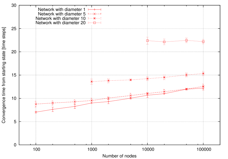
Figure 3: Convergence of network starting from a clean state (geometric random graph, nodes initialized with random values).

4.1 Data Generation

As far as the authors are aware there is no data available in the public domain that describes both the structure and the change in load over some time period for a power grid. To show the effectiveness of our approach we have generated this data ourselves, below we explain how this is done and we show the effectiveness of the proposed distributed algorithm for calculating robustness of an operational grid.

The computation of the system robustness of a power grid requires data describing its topology (i.e., interconnection of nodes with lines), the electrical properties of its components (i.e., admittance values of the transmission lines), information about the nodes (i.e., number and their types), and finally their generation and load values. The IEEE power test systems [18] provide all of these data, the IEEE 118 power system provides a realistic representation of a real world power transmission grid consisting of 118 nodes and 141 transmission lines. We use this as a reference power grid.

The IEEE 118 power system gives information about the topology of the power grid. The loading profile provided with the grid topology [18] gives a representative load for the network, but only for one moment in time. However, in practice, the topology of a power grid remains generally unchanged over time (except for the maintenance, failure and extension of the grid) while the generation/loading profile varies over time. This changing nature of the loading profile (and accordingly the generation profile) results in a varying robustness of the system over time. Therefore simulating the robustness profile of a power grid for a whole day requires a demand profile belonging to the whole day.

To obtain a varying robustness for the IEEE 118 power system, we randomly choose 10% of the power generation nodes of the power system which are then fed with synthetic (generated) demand profiles. The demand values of other power generation nodes remain unchanged. The demand profiles are generated based on an actual load profile for a day of the Dutch grid on January 29, 2006. The demand at the corresponding point in the Dutch grid is sampled per 15 minutes during the whole day. Figure 2 shows the demand profile. Based on this actual demand profile, additional synthetic demand profiles are generated by (i) first introducing random noise to the actual demand profile, and (ii) then by smoothing the curve out with a moving average [21] with a window size of 10. Figure 2 illustrates the actual demand profile and two other synthetically generated demand curves.

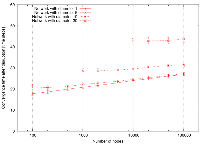
Figure 4: Convergence of network after a disruption (geometric random graph, half of the nodes change their values after initial network convergence).

4.2 Influence of Communication Topology

The underlying communication network for a smart grid can be implemented in a number of ways, mapping to different communication topologies. For example, one might choose to use the internet backbone, allowing any-to-any communication in the network, leading to a fully connected graph. In the first experiment, we have initialized the network with a set of random variables and recorded the time when the aggregated sum converges to the same value on all nodes. As seen in Figure 3, fully connected networks lead to the fastest aggregate computation. In a second experiment, once the network stabilized, we introduced a change in the form of half of the nodes in the network changing their value to a different one. Again, we recorded the time until the network stabilized after this change. As expected, Figure 4 shows that fully connected networks stabilize the fastest after a disruption.

These results assume the internet backbone to work perfectly and able to route the high level of traffic generated. A more realistic scenario is considering that the various data collection points obtain data from the individual consumers via some radio technology (for example GPRS modems) and are themselves connected to the internet backbone. To keep the traffic in the network to a minimum, the data collection points only communicate with their network-wise first order neighbors, leading to a mesh network deployment type. As seen in Figure 3 and Figure 4, the diameter of the network clearly has the major impact factor on the results, confirming the theoretical convergence results. The information needs at least $O(D)$ time steps to propagate through the network. The constant in the $O()$ notation is influenced on one hand by the average connectivity in the network (a node can only contact a single neighbor per time step, slowing information dissemination) and the push-pull communication model on the other (a node may be contacted by several neighbors during a time step, speeding up information dissemination).

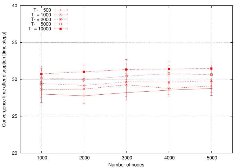
Figure 5: Influence of $T$ parameter (random geometric graph, 10-hop network, half of the nodes change their values randomly after initial network convergence).

4.3 Scalability Aspects

One of the main characteristics of our approach is that the algorithm we propose scales very well with the number of nodes in the network. As seen again Figure 3 and Figure 4, the number of nodes has little influence in the final results (influencing only as $O(\log N)$). The simulation explored a space in which we varied the number of nodes over four orders of magnitude and the results hint that tighter boundaries might exist then the ones we proposed in this paper. We noticed that for a fully connected network, the recovery time varies with $34\%$ between a network with 1000 nodes and one with 100000 nodes, while the variation drops to a mere $2.4\%$ for a 20-hop network varying from 1000 nodes to 100000 nodes.

These results are very important for the smart grid application type. As the network will be linked to a physical space (a country or in general, a region), fully covering it, the diameter of the network is expected to, at most, decrease with the addition of new nodes. Intuitively, when thinking of nodes as devices with a fixed transmission range, adding more devices in the same region may lead to shorter paths between various points. The aggregate computation approach we propose shows on one hand an almost invariance to the increase in the number of nodes in the network and a linear variation with the diameter. These properties are essential for any solution that needs to take into account that the number of participants in the grid will most likely increase over time.

We are also interested in understanding the effects the time-to-live of the negative fields has on the convergence and scalability properties. We have considered a 10-hop network with 1000 to 5000 nodes and varied the time-to-live for negative values between 500 and 10000. Figure 5 confirms Lemma 3.1 with respect to the $\log T$ term. As the data shows, the convergence time was affected very little by the chosen parameters. As expected, the diameter of the network has the larger influence in this mechanism.

4.4 Robustness Metric Computation

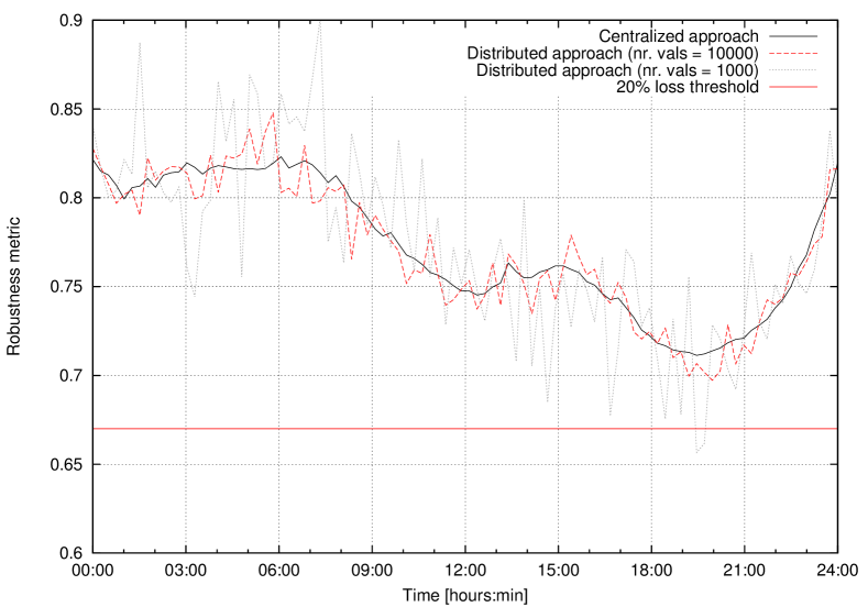
Figure 6: Robustness metric (centrally computed values versus two runs of the distributed algorithm, synthetic data - see Section 4.1, each point represents network data after convergence; the line $R_{CF}=0.67$ illustrates a critical threshold below which line failures can lead to large blackouts in this particular network).

Figure 6 shows the distributed computation method performing with real data sets, obtained through the method described in Section 4.1. We plotted the results of two simulation runs versus the ground truth data, obtained via centralized computation. The length of the value vector was varied from 1000 values to 10000 values, the results confirming that precision can be set to the desired value, independent of the network topology and size. When using a vector of 1000 elements, we obtained a mean relative error of $3\%$ (maximum relative error $11\%$ with a standard deviation of $2.6\%$). Using a larger vector (10000 elements) we were able to obtain a mean relative error of $1\%$ (maximum relative error of $4\%$ with a standard deviation of $0.8\%$). These figures are very good, taking into account that they result from a combination of distributed computations with all the fault tolerant mechanisms enabled.

The figure also includes a line (with robustness value 0.67) that illustrates the critical threshold, set by the grid operator. If the robustness metric drops below this value then a power line failure can lead to a blackout that effects more then 20% of the power grid. This threshold value was obtained by running cascading failure simulations on the IEEE 118 power grid system using targeted attacks (i.e., we considered a worst case scenario). We refer to [25] for a structured methodology for determining such thresholds.

The critical threshold chosen above, that effects more 20% of the power grid, is more or less arbitrary and mainly chosen for illustration purposes. In practice various other factors have to be taken into account by grid operators (line capacities, maintenance cycles) to determine realistic threshold values, but this should illustrate the feasibility of the approach as it clearly shows that the error rate of the distributed algorithm is much smaller then minimal required drop in robustness value that is needed to meet the threshold.

Besides the quantitative values shown in Figure 6 we would like to point that our approach is different from traditional approaches that try to capture the global state of the network and then take decisions centrally (see Section 5). Our approach pushes the computation of the robustness metric in the network, its results being available at each node as soon as the computations converge. This mechanism can be easily used as a measurement phase, leading to the possibility of implementing distributed control loops on top of it.

5 Monitoring and Cascading Failures in Power Grids

Three types of related work on monitoring the state of a power grid can be distinguished: (i) metrics that aim to quantify the vulnerability of the power grid against cascading failures, (ii) simulation models that aim to predict the impact of node/line outages and (iii) sensor networks that aim to capture the operative state of the power grid.

There exists a significant body of work on defining metrics that assess the vulnerability of the power grid against cascading failures. Most studies deploy a purely topological or an extended topological approach mainly relying on graph theoretical measures such as betweenness centrality [34]. However, these studies [22, 10, 7, 8] only focus on the topological properties of power grids and fail to take the operative state of the network into account. In effect this means that such metrics cannot be used to assess the change in vulnerability of operational power grids. In addition to these topological approaches, others [37, 4] propose measures relying on simulation models. Although, these metrics incorporate also the operative state of a power network, it is very challenging to deploy them to quantify the system’s resilience against cascading failures in (near) real-time because their computation requires full knowledge of the power grid state in order to simulate cascades. Our earlier work [24, 23] (also see Section 2) forms a noticeable exception to this, since it defines a metric that considers both the topological and the operative state of a power grid, while not requiring any computationally expensive tasks (e.g., computing the full network state in order to simulate cascades in the network).

Grid operators traditionally assess the network operation by relying on flow based simulation models (i.e., N-x contingency analysis [14]). These models take the operational behavior of the power grid into account. Grid operators can calibrate the model to match the power grid of interest and run various scenarios to assess the impact of one or two lines failing. There are two problems with such tools: they depend on the knowledge of the grid operator who determines which failure scenarios to explore. In addition, due to the complexity of the simulation models it is typically not possible to run scenarios where more than two components fail. The monitoring approach proposed in this paper may complement current grid operator practices.

There are numerous papers that describe distributed architectures that can be used to monitor the state of the power grid. However, these typically focus on the issue of data collection [38, 36, 17, 11, 3, 29, 39, 16] (i.e., loading levels of power lines, phase angles etc.) and do not use any meaningful data aggregation mechanisms to quantify the resilience with respect to cascading failures of the whole power grid. In conclusion, as far as the authors are aware, there are no power grid monitoring approaches that assess the vulnerability, with respect to cascading failures, of an operational power grid in near real-time.

6 Conclusions

In this paper we introduced a novel distributed computation framework for network aggregates and showed how it can be used to assess the resilience with respect to cascading failures of an operational power grid in near real-time. We have enhanced a class of fast gossiping algorithms [9] with self-stabilizing mechanisms to counter run-time network dynamics. To showcase the capabilities of our approach, we exemplified how the robustness metric introduced in [23, 24] can be computed fast and reliable in a distributed network - IEEE 118 power grid.

Our contribution has a number of desirable properties such as scalability and robustness. Simulation results performed with both real and synthetic data show that our approach achieves very fast convergence times, influenced mainly by the diameter of the network and only logarithmically by the number of nodes in the network. This property is very important in the context of smart grids, where the number of nodes deployed over a given area (a region or a country) is expected to increase in the next few decades.

The precision of the computations can be fixed by modifying the size of the messages exchanged in the network. This is a crucial property for scalability, as the size of the messages is not a function of the number of nodes in the network. More importantly, the computation error scales as $O(1/poly(N))$, meaning that the more nodes a network has, the smaller the final error is. Finally, our scheme preserves the anonymity of the participants in the network, as it does not rely on unique identifiers for the nodes of the network.

The main message of this paper can be summarized in that we showed that it is possible to compute complex aggregates of the operational state of the nodes in a network in a fully distributed manner, fast and reliable at runtime. As automatic control systems always include a measurement phase, we see our contribution as the perfect candidate for the measurement block for an automated distributed control scheme. While this paper focused on the measurements of network properties, future work will investigate the actuation part triggered by the availability of results given by different power grid metrics.

References

- [1] R. Albert, I. Albert, and G. L. Nakarado. Structural vulnerability of the North American power grid. Physical Review E, 69:25103, 2004.
- [2] R. Arditi and L. R. Ginzburg. Coupling in predator-prey dynamics: Ratio-dependence. Journal of Theoretical Biology, 139(3):311 – 326, 1989.
- [3] D. E. Bakken, C. H. Hauser, H. Gjermundrød, and A. Bose. Towards more flexible and robust data delivery for monitoring and control of the electric power grid. School Elect. Eng. Comput. Sci., Washington State University, Tech. Rep. EECS-GS-009, 2007.
- [4] Z. J. Bao, Y. J. Cao, G. Z. Wang, and L. J. Ding. Analysis of cascading failure in electric grid based on power flow entropy. Physics Letters A, 373:3032–3040, 2009.
- [5] V. Belevitch. Summary of the history of circuit theory. Proceedings of the IRE, 50(5):848–855, 1962.
- [6] N. Bicocchi, M. Mamei, and F. Zambonelli. Handling dynamics in diffusive aggregation schemes: An evaporative approach. Future Generation Computer Systems, 26(6):877–889, 2010.
- [7] E. Bompard, R. Napoli, and F. Xue. Analysis of structural vulnerabilities in power transmission grids. International Journal of Critical Infrastructure Protection, 2(1-2):5–12, 2009.
- [8] Bompard, Ettore and Napoli, Roberto and Xue, Fei. Extended topological approach for the assessment of structural vulnerability in transmission networks. IET Generation, Transmission and Distribution, 4:716–724, 2010.
- [9] S. Boyd, A. Ghosh, B. Prabhakar, and D. Shah. Gossip algorithms: Design, analysis and applications. In INFOCOM 2005. 24th Annual Joint Conference of the IEEE Computer and Communications Societies. Proceedings IEEE, volume 3, pages 1653–1664. IEEE, 2005.
- [10] X. Chen, Q. Jiang, and Y. Cao. Impact of characteristic path length on cascading failure of power grid. In Power System Technology, 2006. PowerCon 2006. International Conference on, pages 1–5, 2006.
- [11] L. Dan, H. Fukun, G. Ziming, et al. Wide-area real time dynamic security monitoring system of north china power grid. Power System Technology, 28(23):52–56, 2004.
- [12] I. Dobson, J. Chen, J. S. Thorp, B. A. Carreras, and D. E. Newman. Examining criticality of blackouts in power system models with cascading events. In Hawaii International Conference on System Sciences, 2002.
- [13] A. El-Sakkary. The gap metric: Robustness of stabilization of feedback systems. Automatic Control, IEEE Transactions on, 30(3):240–247, 1985.
- [14] R. B. et al. Vulnerability assessment for cascading failures in electric power systems. In Power Systems Conference and Exposition, PSCE, IEEE, 2009.
- [15] L. C. Freeman. A set of measures of centrality based on betweenness. Sociometry, pages 35–41, 1977.
- [16] A. P. Grilo, P. Gao, W. Xu, and M. C. de Almeida. Load monitoring using distributed voltage sensors and current estimation algorithms. Smart Grid, IEEE Transactions on, 5(4):1920–1928, 2014.
- [17] V. C. Gungor, B. Lu, and G. P. Hancke. Opportunities and challenges of wireless sensor networks in smart grid. Industrial Electronics, IEEE Transactions on, 57(10):3557–3564, 2010.
- [18] IEEE test systems data. Available at: http://www.ee.washington.edu/research/pstca/.
- [19] M. Jelasity, A. Montresor, and O. Babaoglu. Gossip-based aggregation in large dynamic networks. ACM Transactions on Computer Systems (TOCS), 23(3):219–252, 2005.
- [20] G. Jesi, D. Hales, and M. van Steen. Identifying malicious peers before it’s too late: A decentralized secure peer sampling service. In Self-Adaptive and Self-Organizing Systems, 2007. SASO ’07. First International Conference on, pages 237–246, July 2007.
- [21] J. Kenney and E. Keeping. Mathematics of Statistics, Pt. 1, chapter 14.2 "Moving Averages", pages 221–223. Princeton, NJ, 1962.
- [22] C. J. Kim and O. B. Obah. Vulnerability assessment of power grid using graph topological indices. International Journal of Emerging Electric Power Systems, 8:1–15, 2007.
- [23] Y. Koç, M. Warnier, F. M. T. Brazier, and R. E. Kooij. A robustness metric for cascading failures by targeted attacks in power networks. In In proceedings of the 10th IEEE International Conference on Networking, Sensing and Control (ICNSC’13), pages 48–53, Piscataway, NJ, USA, 2013.
- [24] Y. Koç, M. Warnier, R. E. Kooij, and F. M. T. Brazier. An entropy-based metric to quantify the robustness of power grids against cascading failures. Safety Science, 59(8):126–134, 2013.
- [25] Y. Koç, M. Warnier, P. Van Mieghem, R. E. Kooij, and F. M. T. Brazier. A topological investigation of phase transitions of cascading failures in power grids. Physica A: Statistical Mechanics and its Applications, 2014 (to appear).
- [26] G. M. Masters. Renewable and efficient electric power systems. John Wiley & Sons, 2013.
- [27] P. McDaniel and S. McLaughlin. Security and Privacy Challenges in the Smart Grid. IEEE Security and Privacy, 7(03):75–77, 2009.
- [28] D. Mosk-Aoyama and D. Shah. Fast distributed algorithms for computing separable functions. Information Theory, IEEE Transactions on, 54(7):2997–3007, 2008.
- [29] K. Moslehi and R. Kumar. A reliability perspective of the smart grid. Smart Grid, IEEE Transactions on, 1(1):57–64, 2010.
- [30] A. E. Motter and Y.-C. Lai. Cascade-based attacks on complex networks. Phys Rev E, page 065102, 2002.
- [31] A. Pruteanu and S. Dulman. Lossestimate: Distributed failure estimation in wireless networks. Journal of Systems and Software, 85(12):2785–2795, 2012.
- [32] D. Shah. Gossip algorithms. Now Publishers Inc, 2009.
- [33] M. Vaiman, K. Bell, Y. Chen, B. Chowdhury, I. Dobson, P. Hines, M. Papic, S. Miller, and P. Zhang. Risk assessment of cascading outages: Part i; overview of methodologies. In Power and Energy Society General Meeting, 2011 IEEE, pages 1 –10, july 2011.
- [34] P. Van Mieghem. Performance analysis of communications networks and systems. Cambridge University Press, 2006.
- [35] G. Werner-Allen, G. Tewari, A. Patel, M. Welsh, and R. Nagpal. Firefly-inspired sensor network synchronicity with realistic radio effects. In Proceedings of the 3rd international conference on Embedded networked sensor systems, pages 142–153. ACM, 2005.
- [36] Y. Yang, D. Divan, R. G. Harley, and T. G. Habetler. Power line sensornet-a new concept for power grid monitoring. In Power Engineering Society General Meeting, 2006. IEEE, pages 8–pp. IEEE, 2006.
- [37] M. Youssef, C. Scoglio, and S. Pahwa. Robustness measure for power grids with respect to cascading failures. In Proceedings of the Cnet 2011, pages 45–49. ITCP, 2011.
- [38] S. Zanikolas and R. Sakellariou. A taxonomy of grid monitoring systems. Future Generation Computer Systems, 21(1):163–188, 2005.
- [39] H.-T. Zhang and L.-L. Lai. Monitoring system for smart grid. In Machine Learning and Cybernetics (ICMLC), 2012 International Conference on, volume 3, pages 1030–1037. IEEE, 2012.
- [40] N. Zhang, T. Zhou, C. Duan, X.-j. TANG, J.-j. HUANG, Z. LU, and C.-q. KANG. Impact of large-scale wind farm connecting with power grid on peak load regulation demand. Power System Technology, 34(1):152–158, 2010.