Order-disorder transitions in a sheared many body system

Abstract

Motivated by experiments on sheared suspensions that show a transition between ordered and disordered phases, we here study the long-time behavior of a sheared and overdamped 2-d system of particles interacting by repulsive forces. As a function of interaction strength and shear rate we find transitions between phases with vanishing and large single-particle diffusion. In the phases with vanishing single-particle diffusion, the system evolves towards regular lattices, usually on very slow time scales. Different lattices can be approached, depending on interaction strength and forcing amplitude. The disordered state appears in parameter regions where the regular lattices are unstable. Correlation functions between the particles reveal the formation of shear bands. In contrast to single particle densities, the spatially resolved two-particle correlation functions vary with time and allow to determine the phase within a period. As in the case of the suspensions, motion in the state with low diffusivity is essentially reversible, whereas in the state with strong diffusion it is not.

I Introduction

The observation of echoes, i.e. a recovery of the initial state, for spins precessing in a magnetic field upon reversal of the field Hahn (1950); Carr and Purcell (1954) and for dye in viscous fluids Homsy (2008) are among the best known experiments that seemingly defy the expected irreversibility in the evolution of many body systems. Several other examples have followed Niggemeier et al. (1993); Chaiken et al. (1986), and in the context of chaotic dynamical systems the absence of echoes and the inability to return to initial conditions has frequently been used as a test for chaotic dynamics Roberts and Quispel (1992); Casati et al. (1986); Pastawski et al. (1995); Eckhardt (2003). While in all these cases the strength of the echoes deteriorates gradually as parameters are varied, the experiments by Pine et al Pine et al. (2005) on sheared suspensions added a new facet to the old problem: they find a phase-transition like change from an essentially reversible state for one set of parameters to an irreversible state for other parameters. Subsequent studies have demonstrated similar transitional behavior in other hydrodynamic experiments Guasto et al. (2010); Metzger and Butler (2012); Jeanneret and Bartolo (2014), particle systems Franceschini et al. (2011); *Franceschini2014; Keim and Arratia (2013); *Keim2013, and complementary simulations Metzger and Butler (2010) and simplified models Düring et al. (2009); Corté et al. (2008, 2009); Menon and Ramaswamy (2009); Keim and Nagel (2011). It has also been put into the context of more general order-disorder transitions in solid materials Mohan et al. (2013); Regev et al. (2013); Fiocco et al. (2013); *Fiocco2014 and granular systems Slotterback et al. (2012); Schreck et al. (2013); Royer and Chaikin (2014). Similar transitions were also reported for superconducting vortices Mangan et al. (2008); Zhang et al. (2010); Okuma et al. (2010); *Motohashi2011; *Okuma2011.

The demonstration of the transition in several other systems suggests that it is a general phenomenon for sheared many body systems. This is also supported by the ability to capture much of the observed behavior and the transition in the discrete time model described in Corté et al. (2008). In order to explore the origin of the phenomenon further and to also establish a connection to reversibility studies in chaotic dynamical systems, we here consider a model for a many-body system that contains some of the features of the suspension experiment but allows for a much more detailed investigation of its long-time properties.

In section II we present the details of the model and demonstrate that it also shows the transition observed in Pine et al. (2005). In section III we characterize the system both before and after the disorder transition. In section IV we investigate the stability properties of the limit cycles described in the previous sections. Finally, in section V we analyze the spatially resolved correlations and their phase dependency. We conclude with a few general remarks and observations in section VI.

II The model and its parameters

For our model we do not aim to calculate the detailed hydrodynamic interaction or exact forces between charged colloids, as done in the simulations of Pine et al. (2005). Rather, we pick an interaction force that captures key features of the fluid-particle system. This is similar in spirit to the model in Corté et al. (2008), but differs in that the model is a continuous one and not an event-driven mapping. We assume that the motion of the many body system is overdamped, so that there is no motion if the external forcing ceases. The forces on the particles are hence balanced by viscous friction, and the equations of motion become

$$\mu\frac{d\mathbf{x}_{i}}{dt}=\mathbf{F}_{i}.$$ (1)

Here, $\mu$ is a friction coefficient, $\mathbf{x}_{i}$ the position of particle $i$, and $\mathbf{F}_{i}$ are the forces acting on the particle. We take the interaction between the particles as repulsive, thereby mimicking the repulsion due to liquid pressure when two particles come close. The particles are confined to a plane, and the domain is taken to be rectangular, and not curved as between the cylinders in the experiments of Pine et al. (2005). The domain is periodically continued in both directions. The main control parameter will be the amplitude of the forcing. A second parameter controls the strength of the interaction between the particles; it is also related to the density of the system, as will be discussed below.

II.1 Forces

The repulsion between the particles is modeled as a potential with power-law decay, $V(r_{ij})\propto r_{ij}^{-\alpha}$, with $r_{ij}$ the distance between particles $i$ and $j$. We here take $\alpha=2$ as a compromise between strong repulsion for short distances (i.e. larger $\alpha$) and a numerically controllable range of the interaction (where hydrodynamics would suggest a decay as slow as $\alpha=1$). With this repulsive interaction, the system is reminiscent of Wigner crystals and clusters of charged particles in plasmas Melzer et al. (1996a); *Melzer1996a; *Schweigert1998. Particle positions are denoted ${\bf x}_{i}=(x_{i},y_{i})$, with $x$ along the direction of shear and $y$ normal to it. The total force acting on the $i$-th particle is the sum of the mutual interactions with all other particles in the system and a periodic shear force in the $x$-direction whose amplitude increases linearly with $y_{i}$,

$$\mathbf{F}_{i}=-\nabla\left(\,\sum\limits_{j\neq i}\frac{A}{\lVert\mathbf{x}_{i}-\mathbf{x}_{j}\rVert^{2}}\,\right)+Sy_{i}\cos(\omega t)\mathbf{e}_{x}.$$ (2)

The parameter $A$ determines the strength of the inter particle potential, $Sy_{i}$ is the amplitude of the shear force and $\omega$ is its frequency. Substituted into equation (1), we obtain the full expression for the time evolution of the position of the $i$-th particle,

$$\frac{d\mathbf{x}_{i}}{dt}=2\frac{A}{\mu}\sum\limits_{j\neq i}\frac{\mathbf{x}_{i}-\mathbf{x}_{j}}{\lVert\mathbf{x}_{i}-\mathbf{x}_{j}\rVert^{4}}+\frac{S}{\mu}y_{i}\cos(\omega t)\mathbf{e}_{x}\,.$$ (3)

II.2 Parameters

In order to expose the independent parameters of the system, we introduce a length scale $\lambda$ and a time scale $T$, and set $\mathbf{x}_{i}=\lambda\mathbf{x}_{i}^{\prime}$ and $t=Tt^{\prime}$. The time $T$ can naturally be identified with the period of the shear, $T=2\pi/\omega\frac{}{}$. The length scale is not related to a quantity explicitly displayed in the equations, but it enters implicitly in the many-body system via the mean distance between particles, and is thus related to the density. Therefore, variations in period and density are absorbed into the two remaining parameters of the system, the dimensionless interaction strength

$$\Gamma_{\mathrm{i}}=2AT/\mu\lambda^{4}$$ (4)

and the dimensionless shear rate

$$\Gamma_{\mathrm{s}}=ST/\mu.$$ (5)

The evolution equations then become

$$\frac{d\mathbf{x}_{i}^{\prime}}{dt}=\Gamma_{\mathrm{i}}\sum\limits_{j\neq i}\frac{\mathbf{x}_{i}^{\prime}-\mathbf{x}_{j}^{\prime}}{\lVert\mathbf{x}_{i}^{\prime}-\mathbf{x}_{j}^{\prime}\rVert^{4}}+\Gamma_{\mathrm{s}}y_{i}^{\prime}\cos(2\pi t)\mathbf{e}_{x}.$$ (6)

We will drop the primes in the subsequent sections and refer to this equation as the evolution equation.

The instantaneous strain $\gamma(t)$ follows from the time evolution of the distance between two particles that initially are displaced by $\Delta y$ perpendicular to the shear. The separation in $x$-direction is then given by $\Delta x(t)=\gamma(t)\Delta y$ with

$$\gamma(t)=\frac{\Delta x(t)}{\Delta y}=\Gamma_{\mathrm{s}}/(2\pi)\sin(2\pi t)=\gamma_{0}\sin(2\pi t)\,;$$ (7)

$\gamma_{0}=\Gamma_{\mathrm{s}}/(2\pi)$ is the amplitude of the affine shear. This also gives a notion of the shear process: At the start of the period, $t=0$, the strain is zero. Over the next half period, the system is tilted to the right, reaching its apex at $t=T/4$. Here, the flow comes to a halt and reverses its direction. After half a period, strain is again zero and the process repeats to the left. The total accumulated strain over one period then becomes

$$\gamma=\int_{0}^{1}\left|\Gamma_{\mathrm{s}}\cos(2\pi t)\right|dt=4\gamma_{0}.$$ (8)

II.3 Numerical implementation

In order to solve equation (6), we introduce Lees-Edwards boundary conditions Lees and Edwards (1972) to account for the sheared images in the $y$-direction. We use a modified minimum image convention, taking several closest images of each particle into account, typically one or two in each direction. The typical number of particles in the main domain is about 100, and in a few examples we went up to 900 particles. Time integration is performed using a 4th order Runge-Kutta-Fehlberg integrator provided by the GNU Scientific Library (GSL). Computation of the right-hand side is parallelized using openMP. The width (in the $x$-direction) of the box is $K$, whereas the height (in the $y$-direction) of the box is $\sin(\pi/3)L$ with $K,L\in\mathbb{N}$ and even and $KL=N$, as suggested by a regular triangular lattice. The simulation was carried out with random initial conditions, and the motion was typically followed over several thousand periods in order to obtain clear evidence for the asymptotic state and to extract reliable statistics in the case of chaotic states.

II.4 Reduced representations and stroboscopic maps

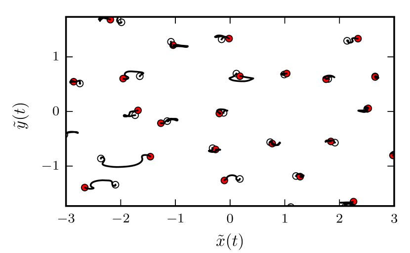
Figure 1: (Color online) Particle trajectories over one period. Initial positions are marked by open circles, final positions by filled red circles. Shown are the reduced positions (9) after subtracting the affine transformation. Non-reversible motions (in particular in the lower left corner) are connected with close encounters and large displacements, see also supplementary movie online Note (1). The parameters are $\Gamma_{\mathrm{i}}=0.1$ and $\Gamma_{\mathrm{s}}=16.0$.

Even for small shear, particles undergo large scale motions along the shear axis, with an amplitude that increases with the displacement in the normal direction. In order to remove this affine deformation, we introduce a reduced representation where the translation by the shear is taken out, i.e. we study

$$\tilde{x}_{i}(t)=x_{i}(t)-\gamma_{0}y(t_{0})\sin(2\pi t)\,.$$ (9)

Figure 1 shows examples of such reduced motions: for the chosen parameters the amplitudes of the motion around the reference positions are small and most particles stay close to their initial positions, but as the group in the lower left corner shows, some of them can experience large displacements as a consequence of close encounters.

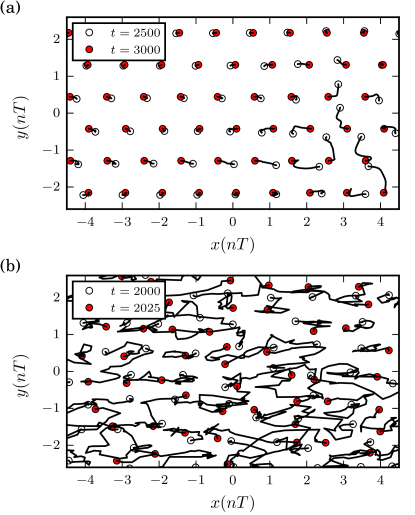
Figure 2: (Color online) Stroboscopic map of particle trajectories for low shear ($\Gamma_{\mathrm{s}}=8$, top) and large shear ($\Gamma_{\mathrm{s}}=16$, bottom). Open circles indicate initial positions, full red circles final positions. In the top diagram for small shear one notes that the particles move very little over the 500 time steps. There is a localized region with larger motions in the lower right corner that is connected with a rare local rearrangement. In the lower diagram for larger shear almost all particles experience large displacements over a much shorter interval of 25 time units. In both cases $\Gamma_{\mathrm{i}}=0.1$.

The long time behavior of the system shows up after a large number of periods only, and is then best studied in the form of stroboscopic maps, with positions taken at multiples of the period, ${\bf x}_{i}(n)={\bf x}_{i}(nT)$. In figure 2 and the accompanying movies we show two examples, one for smaller shear rate and one for larger shear rate. For moderate shear rates, only small displacements are observed and the particles evolve slowly towards regular lattices (section III.1). For larger shear, almost all particles travel larger distances from their initial position. This corresponds to the disordered state of Pine et al. (2005). The random motion of the particles can be captured by diffusion coefficients, which are anisotropic and differ in the longitudinal and transverse directions (section III.2).

III Ordered and disordered states

III.1 Ordered states

In the absence of external forcing, the interactions between the particles push a random initial condition towards a force equilibrium. A regular lattice, such as a hexagon, is an example of such an equilibrium, but it will rarely be reached from a random initial condition since particles will be trapped in a state with a few dislocations or in a state showing several oriented patches, separated by grain boundaries.

As soon as shear is added to the system, the particles will start to rearrange and to self-organize. After sufficiently long times, states like the ones shown in Fig. 3 for $\Gamma_{\mathrm{s}}=2$, $6$, and $8$ are obtained. For very low shear rates the system settles into the hexagonal configuration, with an orientation relative to the shear direction that depends on the initial conditions. Since the regular hexagonal state is a possible force-equilibrium, the external forcing can be seen as a minor perturbation that hardly affects particle interactions. With increasing shear rate, the lattice orientation may change, and the lattice will align parallel or perpendicular to the external force. At a shear rate around $6$, the asymptotic state is given by a rectangular lattice configuration. At $\Gamma_{\mathrm{s}}\approx 8$, we again observe a hexagonal lattice, though this time it is almost always oriented parallel to the shearing motion. Increasing the rate further the system will at some point fail to approach a regular lattice, and a chaotic, disordered state is attained.

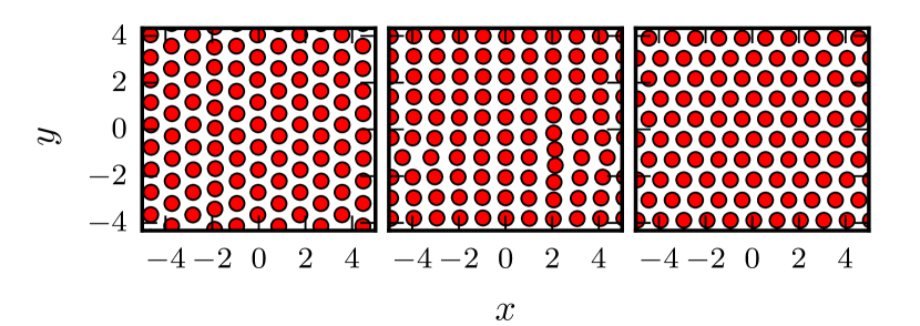
Figure 3: (Color online) Asymptotic states at moderate shear rates, $\Gamma_{\mathrm{s}}=2$, $6$ and $8$, respectively. Except for minor defects they are either a hexagonal or a rectangular lattice configuration. $\Gamma_{\mathrm{i}}=0.1$ in all three cases.

Since the asymptotic reversible states are also lattice configurations, the external forcing only causes affine deformations of the system. This is in contrast to the observations by Keim and Arratia (2014) who found clusters of particles subject to non-affine deformations in the reversible regime. We only observe non-affine deformations in the irreversible regime and in the trajectories approaching the ordered states.

The regular states observed here are a consequence of the homogeneity of the system, the density, and the domain size: Imperfections will most likely trap the system in a glassy or disordered state, as in the experiments of Pine et al. (2005). Another important aspect is the different kind of interactions considered in Pine et al. (2005); Corté et al. (2008). Since there an interaction between particles takes place upon contact only, reversibility is attained as soon as each particle has cleared a sufficiently large space around it. In our case, particles interact over longer distances so that further ordering is required and eventually ordered states are attained. Nevertheless, as Corté et al. (2008) pointed out, very similar absorbing states exist in their systems as well, but are not found by the simulations. Similar to our case, they become unstable as soon as a critical strain is exceeded.

In order to quantify the ordering we investigate the orientation number of an ensemble, defined by

$$\Psi_{k}=\left\langle\frac{1}{k}\sum_{j=1}^{k}\exp\left(\mathrm{i}k\Theta_{ij}\right)\right\rangle.$$ (10)

Here, $k$ is the number of next neighbors taken into account, and $\Theta_{ij}$ is the angle of the vector between particles $i$ and $j$ towards the $x$-axis. Of particular interest are the values of $|\Psi_{6}|$, which becomes unity for a hexagonal lattice, and of $|\Psi_{4}|$, which becomes unity for a rectangular lattice.

We show the results in Fig. 4 for a wide range in parameter space $\Gamma_{\mathrm{i}}\times\Gamma_{\mathrm{s}}$. For low shear rates and independent of the interaction strength, the orientation number reflects the previously mentioned change of the asymptotic states. For very low shear rates up to $\Gamma_{\mathrm{s}}\lesssim 3$ and for shear rates larger than $\Gamma_{\mathrm{s}}\gtrsim 7$, a hexagonal lattice is preferred. For shear rates in between we find $|\Psi_{4}|\approx 1$, and thus a rectangular lattice is attained. With increasing shear rate and low enough interaction strength $\Gamma_{\mathrm{i}}$, order is lost beyond $\Gamma_{\mathrm{s}}\gtrsim 11$. This corresponds to the observation of chaotic states such as in Fig. 2(b). For a larger interaction strength $\Gamma_{\mathrm{i}}$, ordered states are attained even at large shear rates. However, the computational demand increases and integration times become too short, and hence several defects remain in the configurations and reduce the orientation number. However, in contrast to the orderless region, we find an orientation number which is larger than $0.4$ in this region. Additionally, we observe a modulation of the orientation number with $\Gamma_{\mathrm{s}}$, in which both lattice types alternately dominate.

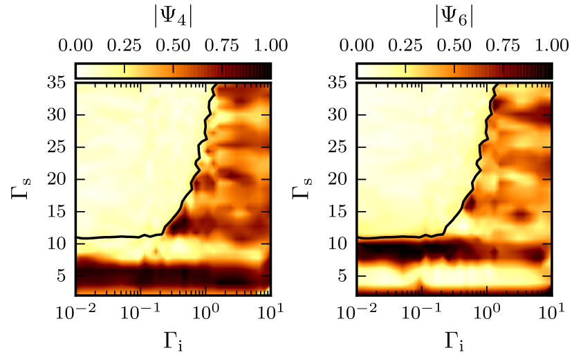
Figure 4: (Color online) Order parameters $|\Psi_{4}|$ and $|\Psi_{6}|$ for different values of $\Gamma_{\mathrm{i}}$ and $\Gamma_{\mathrm{s}}$. For a low shear rate $\Gamma_{\mathrm{s}}$ we clearly observe a change from sixfold orientation to fourfold orientation (at $\Gamma_{\mathrm{s}}\approx 3$) and back to sixfold orientation (at $\Gamma_{\mathrm{s}}\approx 7$). In the light area in the upper left, no ordering of any kind is observable. Its lower boundary is located near $\Gamma_{\mathrm{s}}\approx 11$. For larger $\Gamma_{\mathrm{i}}$, the system attains lattice configurations even at larger shear rates. Although the system then does not reach perfect lattice configurations, a modulation with $\Gamma_{\mathrm{s}}$ is still discernible. The black solid lines indicate the loss of ordering where both $|\Psi_{4}|$ and $|\Psi_{6}|$ drop below $0.4$.

III.2 Diffusion constants

Convenient scalar quantities that can be used to distinguish the different long-time dynamics are related to the diffusive motions of the particles. The local and instantaneous quantity is the mean displacement of particles over one period,

$$\delta s(n)=\frac{1}{N}\sum_{k=1}^{N}{}\left\|{\bf x}_{k}(n)-{\bf x}_{k}\left(n-1\right)\right\|$$ (11)

It provides a convenient measure to quickly distinguish between regular and irregular states, as shown in Fig. 5. For large shear ($\Gamma_{\mathrm{s}}=16$) the displacement is large and varies little in time, indicating a disordered, chaotic state. For low shear ($\Gamma_{\mathrm{s}}=8$) it decreases, eventually reaching machine precision: the system evolves towards a stable state. The intermediate maxima, such as the one near $t=2800$ in Fig. 5, indicate reorganizations to remove lattice defects. The event is related to the rearrangement in the lower right corner in Fig. 2 (top) and clearly visible in the movie Note (1).

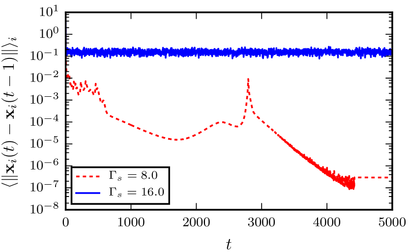
Figure 5: (Color online) Average displacement after one period for different shear rates $\Gamma_{\mathrm{s}}$. For low shear rates, it drops to numerical precision with intermediate bumps indicating reorganizations. For large shear rates, the average displacement approaches a finite value reflecting the random motion. $\Gamma_{\mathrm{i}}=0.1$.

In the diffusive state, we can calculate diffusion constants. In view of the asymmetry in the system in the directions along the shear and perpendicular to it, we consider two separate diffusions constants. The diffusion constants can be obtained either by averaging in time over the displacements over one period,

$$2D_{x}\gamma=\left\langle\frac{1}{N}\sum_{k=1}^{N}{}\lvert x_{k}(n)-x_{k}\left(n-1\right)\rvert^{2}\right\rangle_{n>n_{\mathrm{transient}}}$$ (12)

or by approximating the mean square displacement of the particles by a straight line,

$$\langle\Delta x^{2}(n)\rangle=2D_{x}\gamma n.$$ (13)

The factor $\gamma$ is adopted from the definitions in Pine et al. (2005). Expressions for the diffusion constant in the $y$-direction are obtained by replacing $x_{k}$ by $y_{k}$. Due to the slightly different definitions, we call eqn. (12) short term diffusivity, and eqn. (13) the long term diffusivity. The averages are taken after initial transients have decayed. The number of periods one has to wait depends on the system size and the asymptotic behavior: While in the disordered regime, the system approaches its final state quickly, this time may be several thousand periods when the system approaches an ordered configuration. This shows up in $\delta s$, which can be used to distinguish ordered from disordered states. For disordered states, the diffusion constant is obtained by averaging over $10^{3}$ to $10^{4}$ periods. In the ordered states, the diffusion constant calculated from averages over shorter time intervals shows a drop towards zero.

Since the simulation of large ensembles is computationally expensive, we concentrate on a system size of $N=100$ from here on. To verify that the results are not affected by the system size, we occasionally investigate systems of sizes $N=400$ and $900$ for a few parameter values. While the results for the diffusion constants seem to be independent of the system size as shown below, the time for transients to decay increases rapidly with system size and adds to the numerical challenges.

III.3 Transitions for fixed $\Gamma_{\mathrm{i}}$

We begin the exploration of the parameter space of the system with a fixed interaction parameter $\Gamma_{\mathrm{i}}=0.1$ and different shear rates $\Gamma_{\mathrm{s}}$. We compare both short term and long term diffusivities in Fig. 6. As anticipated from the results in the previous section, we notice two qualitatively different states that can be distinguished by their diffusion constants. In one case, the system approaches a state with zero diffusivity and reversible motion. In the other case, the diffusivity does not vanish and the motion is irreversible. For this specific set of parameters, we computed the diffusivities both for a 100 and a 900 particle system. Up to a shear rate of $\Gamma_{\mathrm{s}}$ just above 30.0, the results are in very good agreement. Beyond this value, the system with 100 particles gives slightly higher values. This is most likely caused by finite size effects: At $\Gamma_{\mathrm{s}}=36$, which corresponds to a strain amplitude $\gamma_{0}=5.73$, particles separated by $\Delta y=\sqrt{3}/2$ in the normal direction are advected by one box length relative to each other. Therefore, at the left and right turning points of the shearing motion, particles experience the same neighborhood.

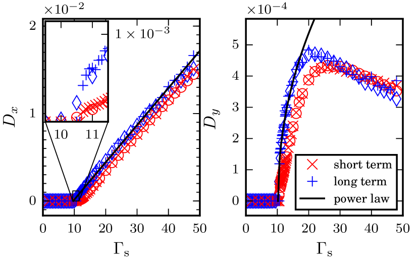
Figure 6: (Color online) Diffusivities along the $x$- and $y$-direction, left and right panel respectively, for $\Gamma_{\mathrm{i}}=0.1$. Additional data of a 900-particle systems is marked by open symbols (short term: $\circ$; long term: $\diamond$). For low shear rates, no diffusion is observed, corresponding to a reversible state. At a critical point $9.5<\Gamma_{2,\mathrm{c}}<10.5$ diffusions start to grow, both parallel and perpendicular to the shear, corresponding to an irreversible state. The inset in the left panel shows a magnification of the critical region. The short term diffusivity is slightly smaller than the long term diffusivity. Moreover, diffusion parallel to the shear is strongly enhanced and shows a different behavior: It grows linearly with increasing shear whereas diffusion in the perpendicular direction saturates. Boundary effects due to the system size seem to be negligible up to $\Gamma_{\mathrm{s}}\approx 30.0$ since data points for $100$ and $900$ particles coincide well.

The transition between reversible and irreversible motion as the shear rate is varied shows up rather clearly. For $\Gamma_{\mathrm{i}}=0.1$, this transition takes place near $\Gamma_{\mathrm{s}}\approx 10.5$. Fitting a power law of the form $D=\delta\left(\Gamma_{\mathrm{s}}-\Gamma_{2,\mathrm{c}}\right)^{\beta}$ returns an exponent $\beta_{x}=1.00$, a critical value $\Gamma_{2,\mathrm{c}}^{x}=9.6$ for the diffusivity in the shear direction, and $\beta_{y}=0.47$ and $\Gamma_{2,\mathrm{c}}^{y}=10.2$ for the diffusivity in the normal direction. The values for the critical shear rate are lower than the point where a non-zero diffusivity is first observed. The inset in Fig. 6 shows this critical region in more detail. A closer inspection of the diffusivities near the critical point reveals that they drop to zero abruptly. This suggests a small region where ordered and disordered motions coexist, so that the transition could be subcritical and hysteresis effects might be observed. Unexpected are the differences in the exponents: Parallel to the shear direction, the diffusivity grows linearly with the shear, but perpendicular to it, the diffusivity varies with a square root. Overall, the sharp transition is in qualitative agreement with the results both from experiments and simulations, e.g. Pine et al. (2005); Metzger and Butler (2010); Guasto et al. (2010).

We find that the short term diffusivity eqn. (12) is slightly lower than its long term counterpart. Parallel to the shear direction, the difference approaches a constant value, whereas in the perpendicular direction, it diminishes for larger shear rates. Our interpretation is that on short time scales, each particle is captured in a matrix of surrounding particles. Their presence introduces memory and correlations into the process, thereby reducing the diffusion coefficient. This effect is most pronounced in the parameter range close to the transition and becomes weaker with increasing shear.

III.4 Anisotropy in diffusion

We also notice that horizontal diffusivities are much stronger than vertical ones. This is due to the shear acting only along the $x$-direction and was also observed in other investigations on similar systems Pine et al. (2005); Metzger and Butler (2010). Moreover, for larger shear rates, the vertical diffusivity seems to approach a fixed value whereas the horizontal diffusivity grows linearly over the investigated parameter range. This phenomenon of enhanced diffusion is known as advection-diffusion coupling and has been studied for the case of Brownian motion in a shear flow by Young et al. (1982). They showed that the diffusion constants are related to each other by

$$D_{x}=D_{x,0}+\frac{1}{2}\gamma_{0}^{2}D_{y},$$ (14)

where $\gamma_{0}$ is the strain amplitude. Thus, parallel diffusion is enhanced by a coupling between normal diffusion and shearing. The bare longitudinal diffusivity without this effect is denoted $D_{x,0}$. The mechanism can be illustrated in a three step process by decoupling diffusion and advection: In the first step, we observe diffusion perpendicular to the shear so that particles are found in the layer above. In the next step, this layer is advected by the shear over some distance. In the last step, particles in the upper layer diffuse back to the original layer. Since they have been transported by the flow, they have traveled further than by horizontal diffusion alone. Equation (14) shows that for an isotropic system the bare longitudinal and transversal diffusivities coincide.

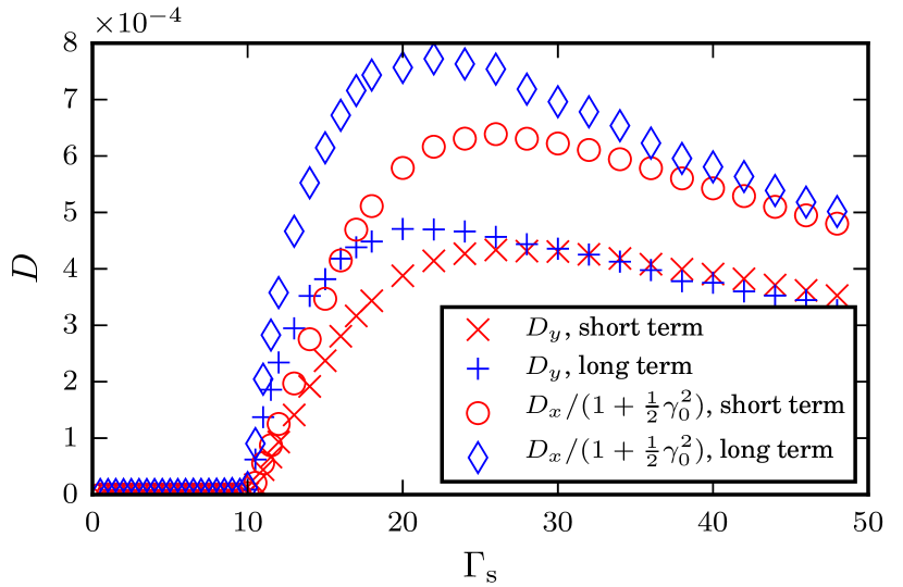
Figure 7: (Color online) Relation of the corrected parallel diffusivity (eqn. (14)) to the perpendicular diffusivity. The rescaled parallel diffusivity is still stronger, indicating a true anisotropy. Data was taken from the 900-particle system.

In Fig. 7, we show the corrected parallel in relation to the perpendicular diffusivity. Data was taken with the 900-particle system. We consider $D_{x}/(1+\frac{1}{2}\gamma_{0}^{2})$, which in the limit of large $\gamma_{0}$ should approach $D_{y}$. We observe that the bare parallel diffusivity is noticeably larger than the perpendicular diffusivity, contrary to the expectations for an isotropic system. Moreover, we can extract a factor between the two of approximately $1.5$ over the whole range, even in the limit $\Gamma_{\mathrm{s}}\approx 50$, i.e. $\frac{1}{2}\gamma_{0}^{2}\approx 32$. This suggests that the bare horizontal diffusivity $D_{x,0}$ grows with shear rate. We confirmed that this behavior is not affected by boundary conditions by repeating the simulations in a quadratic box where we found the same increase.

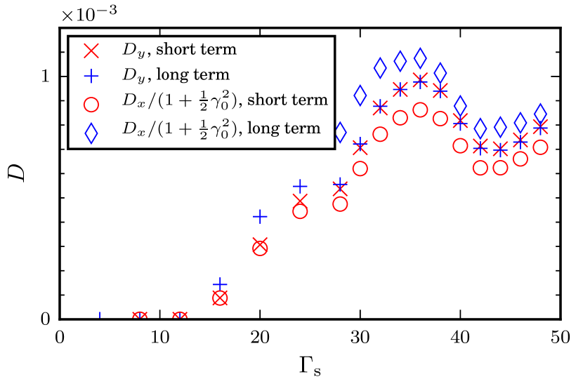
Figure 8: (Color online) (Rescaled) diffusivities at $\Gamma_{\mathrm{i}}=1.0$. Below $\Gamma_{\mathrm{s}}=28$, the simulation has not converged towards the asymptotic ordered state: While most particles are arranged in a lattice structure, multiple defects exist which slowly grow out. Therefore, the long term diffusivity strongly deviates from the short term diffusivity and is neglected. At larger shear rates, we observe good agreement with eqn. (14), i.e. the anisotropy is caused by advection-diffusion coupling.

The differences between bare longitudinal and transverse diffusion disappear for stronger interactions $\Gamma_{\mathrm{i}}$. The diffusivities for $\Gamma_{\mathrm{i}}=1.0$ in an ensemble of 900 particles are presented in Fig. 8. On the numerical side, we note that due to the strong interaction and the resulting steeper gradients, integration times increase considerably. Below $\Gamma_{\mathrm{s}}=28$ the system has not yet converged towards an ordered state: While most particles are arranged in a lattice configuration, unordered regions exist which relax only very slowly. This is also reflected in the squared displacements: Instead of approaching a linear growth for larger $\gamma t$, they obey a power law, $\langle\Delta y^{2}\rangle=2D_{y}(\gamma t)^{\alpha}$ with $\alpha>1$. For larger shear rates, the simulation has converged and both the short term and long term diffusivity perpendicular to the strain coincide. Virtually the same applies to the longitudinal diffusivity, though we do not observe perfect agreement. The cause for the deviation is the same as for $\Gamma_{\mathrm{s}}=0.1$, the particles being correlated for a few periods before showing diffusive behavior. The more important observation is that the rescaled diffusivities $D_{x,0}$ in Fig. 8 nicely bracket the perpendicular diffusivity. Thus, for larger $\Gamma_{\mathrm{i}}$ the anisotropy can be completely explained by advection-diffusion coupling.

III.5 Exploration of the $\Gamma_{\mathrm{i}}$-$\Gamma_{\mathrm{s}}$-parameter plane

Next, we turn to the dependence on the shear rate and the interaction strength. In Fig. 9, both parallel and perpendicular diffusivities are shown in a large domain of the parameter space $\Gamma_{\mathrm{i}}\times\Gamma_{\mathrm{s}}$.

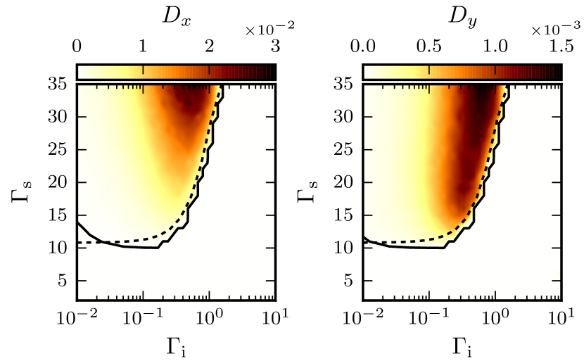
Figure 9: (Color online) The long term diffusion constants $D_{x}$ (left panel) and $D_{y}$ (right panel) for different values of $\Gamma_{\mathrm{i}}$ and $\Gamma_{\mathrm{s}}$. The diffusivity is obtained by fitting data with eqn. (13). The black solid lines indicate $D_{x}=1\times 10^{-5}$ and $D_{y}=1\times 10^{-6}$, respectively. The dashed lines are the smoothed curves taken from Fig. 4, indicating the loss of structural ordering. Results for $\Gamma_{\mathrm{s}}>5\cdot 2\pi$ have to be treated with care due to the limited box-width of $L_{x}=10$: At this point, during one period each particle slips beyond five particles in each direction. This leads to a stabilizing effect for $\Gamma_{\mathrm{i}}>0.5$: Although the shear force is strong, at the turning points of the oscillation the particle interaction still dominates and promotes ordering into a lattice configuration. This behavior is not observed for larger box-sizes.

We observe a distinct boundary where diffusivities become finite as the shear rate $\Gamma_{\mathrm{s}}$ is increased. It nicely corresponds to the boundary determined by the loss of ordering in the system, observed in Fig. 4. For a better comparability, a smoothed representation of the curve where the ordering number $|\Psi_{k}|$ drops below $0.4$ is shown in Fig. 9 as well.

In general, the diffusivity increases with the interaction parameter $\Gamma_{\mathrm{i}}$ up to a critical value where it drops to zero. A small diffusivity $D$ for small values of the interaction parameter $\Gamma_{\mathrm{i}}$ is plausible, since a relatively higher shear rate $\Gamma_{\mathrm{s}}$ is needed to bring particles closer together and to allow the system to display large spatial fluctuations. The dominant force is the external forcing, and after one period the particles are very close to where they were one period before. This leads to a small diffusion constant. In fact, the relaxation time becomes so long that we cannot measure a proper diffusion constant. However, there are qualitative differences depending on the shear rate $\Gamma_{\mathrm{s}}$: For small shear rates, the particles are evenly distributed, but unordered, whereas for larger shear rates the particles are uniformly distributed. This is also supported by two-particle correlation functions. However, the transition between the two regimes is not as sharp as for stronger particle interactions. For large interaction parameters we see a similar behavior, but for a different reason. Since the interaction is comparatively strong, we need a high shear rate to keep the particles away from their equilibrium positions. On the other hand, for large $\Gamma_{\mathrm{i}}$, the settling time scale is shorter, and since the period of the external forcing is fixed to $1$, we expect to find a critical region where particles settle into an ordered state before they can start moving in a random fashion. This is reflected in a relatively sharper transition in Fig. 9 for $\Gamma_{\mathrm{i}}\approx 1$. As would be anticipated, stronger shear rates are required as the particle interaction is increased.

For a dilute solution of particles, Pine et al. (2005) found that the diffusivity is independent of the period of the forcing. In order to check whether our results are independent of the driving period, we have to vary the period while keeping the strain $\gamma$ fixed. With our dimensionless parameters, this corresponds to a variation of $\Gamma_{\mathrm{i}}$, while $\Gamma_{\mathrm{s}}$ is kept fixed. From Fig. 9, we see that for small $\Gamma_{\mathrm{i}}\leq 0.2$, i.e. short enough periods and weak interactions, the onset of a finite diffusivity and the loss of ordering is independent of the driving period. For longer periods and stronger forces though, the interaction between particles has more time to drive the system to the ordered, reversible state.

However, the relation to the experiments of Pine et al. (2005) is more complicated. In the experiments, the shear rate was fixed and the shear amplitude was changed by varying the period. This implies a change in $\Gamma_{\mathrm{i}}$ as well, because the particles have more time to interact. In the fluids context, the interaction comes from the hydrodynamic forces, and they become smaller if the shear rate (and thus the speed) is reduced. The parameter regime where both systems show similar phenomenology then is the range of small $\Gamma_{\mathrm{i}}$, where the transition is determined by $\Gamma_{\mathrm{s}}$ alone.

IV Linear stability analysis

Investigation of the long term trajectories of simulations in the reversible regime show that they approach regular lattices. That regular lattices are force equilibria, even under periodic shear, follows from the fact that to each particle pair there is a corresponding one with opposite forces. More formally, consider a lattice configuration with a point symmetry in particle spacings, i.e. a situation where for every pair $i$, $j$ one can find another pair $i$, $k$, such that $\mathbf{x}_{ij}=-\mathbf{x}_{ik}$. Then it is easy to see that the inter-particle forces in eqn. (6) vanish. Since the shear force only introduces an affine transformation, the force balance stays unaffected during the shear process. Therefore, the regular lattices under shear correspond to a periodic cycle of system (6),

$$\mathbf{x}_{i}^{o}(t)=\mathbf{x}_{i}^{\mathrm{lattice}}+\frac{\Gamma_{\mathrm{s}}}{2\pi}y_{i}^{\mathrm{lattice}}\sin(2\pi t)\mathbf{e}_{x},$$ (15)

for all parameter values $\Gamma_{\mathrm{i}}$ and $\Gamma_{\mathrm{s}}$. The initial regular lattice points are denoted $\mathbf{x}_{i}^{\mathrm{lattice}}$, and their time-dependent cousins are $\mathbf{x}_{i}^{o}(t)$. The regular lattices we consider are the ones obtained under small shear (Fig. 10): the equilateral triangular lattice with particles aligned along the shear direction, the same lattice rotated by $90^{\circ}$, and the rectangular lattice aligned with the shear. In order to determine their stability against small perturbations, we have to perform a Floquet analysis, on account of the periodic variation of the sheared lattices.

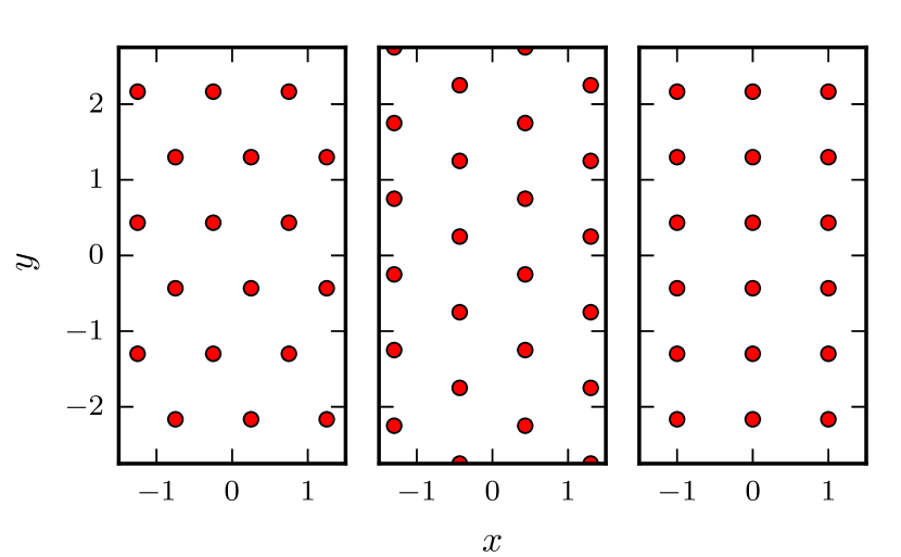
Figure 10: (Color online) The three particle configurations considered in the linear stability analysis, from left to right: equilateral triangular lattice aligned along the $x$- and $y$-axis and rectangular lattice. These are also the asymptotic states found in the dynamical system.

IV.1 Floquet analysis

We linearize the evolution equation (6) around the periodic cycle (15)

$$\mathbf{x}_{i}(t)=\mathbf{x}_{i}^{o}(t)+\mbox{\boldmath$\delta$}_{i}(t).$$ (16)

This yields a system of linear ordinary differential equations for the perturbation vector $\mbox{\boldmath$\delta$}(t)$,

$$\frac{d\mbox{\boldmath$\delta$}}{dt}=\Gamma_{\mathrm{i}}\left(\mathcal{D}(t)-\mathcal{M}(t)\right)\mbox{\boldmath$\delta$}+\Gamma_{\mathrm{s}}\mathcal{S}(t)\mbox{\boldmath$\delta$}=\mathcal{W}(t)\mbox{\boldmath$\delta$}.$$ (17)

The right-hand side of this system consists of a time-periodic coefficient matrix $\mathcal{W}(t)$ composed of $2N\times 2N$ matrices

$$\mathcal{D}(t)=\begin{pmatrix}G_{1}&&0\\ &\ddots&\\ 0&&G_{n}\end{pmatrix},$$ (18)

and

$$\mathcal{M}(t)=\begin{pmatrix}0&B_{1,2}&\dotsb&B_{1,N}\\ B_{1,2}&0&\dotsb&B_{2,N}\\ \vdots&\vdots&\ddots&\vdots\\ B_{1,N}&B_{2,N}&\dotsb&0\end{pmatrix},$$ (19)

where $G_{i}(t)=\sum_{j\neq i}B_{i,j}(t)$ with the $2\times 2$ Jacobi matrices $B_{i,j}(t)$ of the pairwise particle interactions,

$$B_{i,j}(t)=\frac{\openone_{2}}{{\|\mathbf{x}_{i}^{o}-\mathbf{x}_{j}^{o}\|}^{4}}-\frac{4\left(\mathbf{x}_{i}^{o}-\mathbf{x}_{j}^{o}\right)\otimes\left(\mathbf{x}_{i}^{o}-\mathbf{x}_{j}^{o}\right)}{{\|\mathbf{x}_{i}^{o}-\mathbf{x}_{j}^{o}\|}^{6}}.$$ (20)

Here, $\otimes$ denotes the dyadic product and $\openone_{2}$ is the identity-matrix in two dimensions. Finally, we have the Jacobi matrix of the external forcing,

$$\mathcal{S}(t)=\begin{pmatrix}S_{2}(t)&&0\\ &\ddots&\\ 0&&S_{2}(t)\end{pmatrix},\quad S_{2}(t)=\begin{pmatrix}0&\cos(2\pi t)\\ 0&0\end{pmatrix}.$$ (21)

Since the coefficient matrix has a periodic time-dependence, the linear stability analysis requires an integration of the equations over a full period Chicone (2006). To this end, we compute the principal fundamental matrix $\Phi(t)$ of system (17) with initial condition $\Phi(0)=\openone_{2N}$. The matrix after a full period, $\Phi(1)\equiv\Phi$, is the Floquet matrix and is not necessarily a symmetric matrix. The stability properties of system (17) then depend on the eigenvalues of $\Phi$ only. The eigenvalues $\sigma$ of $\Phi$ are called Floquet multipliers. For stability, we require $\lvert\sigma\rvert$ for all possible eigenvalues $\sigma$ of $\Phi$ to be less than one. There are two neutral modes ($\sigma=1$), connected with the invariance of perturbations along the orbit and translational invariance in the $x$-direction.

As an important technical detail we mention that the boundary conditions have to be implemented such that they are compatible with the symmetries of the system so that the symmetries of the matrices are preserved. To this end, we introduce an interaction radius around each particle, and take all interactions with particles inside the circle into account. The radius is chosen to be at least of the order of the box dimensions.

IV.2 Stable and unstable configurations

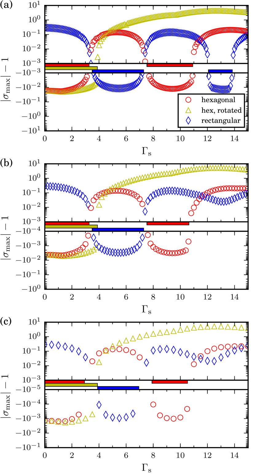
Figure 11: (Color online) The largest eigenvalues $\sigma_{\max}$ of $\Phi$ in dependence on $\Gamma_{\mathrm{s}}$ for the three investigated configurations with $N=100$, $400$, and $900$ particles from top to bottom. Neutral modes are omitted. In each upper panel, markers indicate eigenvalues $|\sigma_{\max}|>1$ and thus unstable configurations, and stable modes ($|\sigma_{\max}|<1$) in the lower panels accordingly. In between, the regions of stability are represented by colored bars. We find that for values of $\Gamma_{\mathrm{s}}\lesssim 11$, linearly stable states exist. Beyond, linear stability is lost. This is in good agreement with the diffusion constant calculated earlier. With increased number of particles, the stable modes become less stable, the qualitative difference between $400$ and $900$ particles being rather marginal. The stable patch at $\Gamma_{\mathrm{s}}>12$ in the 100-particle system can clearly be identified as a finite size effect due to the limited box-width. The value of $\Gamma_{\mathrm{i}}$ is set to $0.1$ in all calculations.

We studied the stability of configurations with $N=100,400$ and $900$ particles. We find that results are qualitatively the same, with the stable modes being closer to unity for more particles. We investigated three different configurations as described above, and for the rotated hexagonal configuration we swapped $L_{x}$ and $L_{y}$.

It turns out that for $\Gamma_{\mathrm{i}}=0.1$, at least one configuration is stable for values of $\Gamma_{\mathrm{s}}\lesssim 10.5$. This value corresponds to a shear rate where each particle is shifted by $1.5$ particle distances in relation to the neighboring rows. For larger values, the periodic cycles remain unstable. The largest multipliers are shown in Fig. 11 for a wide range of the shear rate. We find three regions with different stable configurations. For $\Gamma_{\mathrm{s}}\lesssim 3.5$, both the hexagonal state and its rotated counterpart are stable. Thereafter, the rectangular state is stable up to a shear rate of $\Gamma_{\mathrm{s}}\lesssim 7.5$ until finally the hexagonal configuration is stable again. The changes occur at shear rates corresponding to relative displacements of neighboring rows of approximately $0.5$, $1$ and $1.5$ particle distances. They nicely correspond to the modulations of the orientation number shown in Fig. 4. Only in a small interval at $\Gamma_{\mathrm{s}}\approx 7.5$, all considered lattices appear to be unstable. The inspection of long term trajectories shows, that the system relaxes towards a mixture of both the hexagonal and rectangular lattice and still is in the reversible regime.

The different behavior of the rotated hexagonal configuration can be understood from a geometrical point of view: In the hexagonal lattice with particles aligned along the shear direction, the initial configuration is reproduced after a shear displacement by one particle distance. In the rotated lattice a shift by four particle distances is needed before the lattice returns, corresponding to a shear rate of $\Gamma_{\mathrm{s}}\approx 20$. An analysis of the Jacobian indicates that it picks up strongly unstable modes during this process.

We do not find any qualitative differences between the $400$ and $900$ particle ensemble. Quantitatively, the stable modes become less stable with increasing number of particles. Additionally, the points where the configurations change stability are slightly shifted. The magnitudes of the unstable modes, however, are almost identical. The 100 particle system, on the other hand, clearly shows signs of boundary effects. In the range $12\lesssim\Gamma_{\mathrm{s}}\lesssim 14$, the rectangular lattice becomes stable again. This is neither observed in the larger systems, nor in the simulations. The source might be the limited box width in conjunction with the long range potential. Except for this detail, the 100 particle system qualitatively agrees with the larger ensembles as well.

A variation of the interaction strength $\Gamma_{\mathrm{i}}$ reveals that the location of stable regions is independent thereof for $\Gamma_{\mathrm{i}}\lesssim 0.2$. For a larger interaction strength, more stable regions emerge, in general accordance with Fig. 9. However, the computational demand considerably increases as $\Gamma_{\mathrm{i}}$ is increased, so that a systematic investigation with an adequately large number of particles is unfeasible.

V Particle distributions

V.1 Radial distribution functions

Additional information about the structure of the system that goes beyond the value of the diffusion constants and reversibility can be obtained through correlation functions that contain information about the arrangements of particles. The radially averaged two-particle correlation function counts the number of particles within a ring bounded by the radii $r-\delta r$ and $r+\delta r$, normalized by the mean number of particles in such a ring,

$$g(r)=\frac{1}{N}\frac{\int_{r-\delta r/2}^{r+\delta r/2}\sum_{ij}\delta(r_{ij}-\tilde{r})d\tilde{r}}{\int_{r-\delta r/2}^{r+\delta r/2}2\pi\tilde{r}\rho d\tilde{r}},$$ (22)

where $\rho=N/(L_{x}L_{y})$ is the average particle density of the system. For a crystalline structure, one expects sharp peaks corresponding to the underlying lattice, the first one at the next neighbor distance, and so on. In a liquid state no long range ordering is found so that the correlation approaches one at larger distances. As neighboring particles repel each other, one expects a gap close to the particle and a strong peak at the position of the nearest neighbors. Fig. 12 shows the correlation functions of the system for different shear rates $\Gamma_{\mathrm{s}}$ (and $\Gamma=0.1$). To obtain better statistics all simulations in this section are done for systems of 900 particles. Inspection of the final states and the displacements per particle show that they behave exactly as the smaller systems of 100 particles. Each ensemble is taken at a full period after a total simulation time of 11000 periods, i.e. we assume the system has reached its asymptotic state, which is certainly the case for the systems at larger shear rates.

Figure 12: (Color online) Radial correlation functions of ensembles at different shear rates. For clearer distinction, graphs are shifted by a constant. At low shear rates ($\Gamma_{\mathrm{s}}=6.0$ and $8.0$, respectively), the crystalline structure is reflected by isolated peaks at the next neighbor distances: At $\Gamma_{\mathrm{s}}=6.0$ the rectangular lattice with $a=1.0$ and $b=\sqrt{3}/2$, and the hexagonal lattice with $a=1.0$ at $\Gamma_{\mathrm{s}}=8.0$. At higher shear rates, in the irreversible regime, the correlation function shows features of a liquid: Beyond a minimum distance, the function quickly approaches $1.0$ and displays only small fluctuations. Simulation of 900 particles, $\Gamma_{\mathrm{i}}=0.1$.

As expected, at low shear rates the ordered structure of the state is reflected in the correlation function. At $\Gamma_{\mathrm{s}}=6.0$, we find two superimposed peaks at $r=\sqrt{3}/2$ and $1.0$, corresponding to the rectangular lattice. At a slightly increased shear rate of $\Gamma_{\mathrm{s}}=8.0$ the asymptotic state changes, as can be seen in the correlation function which exhibits isolated peaks at $r=1.0$ and $\sqrt{3}$, corresponding to the next neighbor distances in a hexagonal lattice. At higher shear rates after the motion became irreversible, the correlation function shows features of a liquid: Beyond a minimum distance owing to the repelling potential, the function quickly approaches 1.0 and shows only small modulations. For even larger shear rates, the correlation function becomes featureless except for the next neighbor repulsion: the system is in a gas-like state. However, no spatial information can be extracted in the latter cases. The next neighbor distance is identified as $0.8$ at $\Gamma_{\mathrm{s}}=16.0$, and it decreases to $0.7$ at $\Gamma_{\mathrm{s}}=30.0$. This points to an improvement of the mixing process with increasing shear rate, which leaves the particles less time to relax and to return to larger separations.

V.2 2-d correlation functions

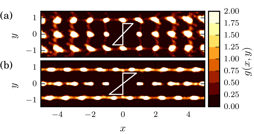
Figure 13: (Color online) The 2-dimensional correlation function $g(x,y)$ at low shear rates. Colors indicate the neighbor density. At the white patches, $g(x,y)$ exceeds $2.0$. Just as the radial correlation function $g(r)$, $g(x,y)$ reflects the crystalline structure: At $\Gamma_{\mathrm{s}}=6.0$, (a), we observe the rectangular lattice structure, whereas at $\Gamma_{\mathrm{s}}=8.0$, (b), the hexagonal lattice is recovered. In both cases, the blur is caused by minor lattice defects whereby in the latter case almost perfect vertical alignment is observed. The white triangles indicate how far the populated rows have been sheared against each other over the past quarter period. They are set at arbitrary height such that features of the correlation function are not occluded. Simulation of 900 particles, $\Gamma_{\mathrm{i}}=0.1$

In order to obtain more spatial information, we now turn to the spatially resolved two-particle correlation function

$$g(x,y)=\frac{1}{n}\iint_{\begin{subarray}{c}x-\delta x/2\\ y-\delta y/2\end{subarray}}^{\begin{subarray}{c}y+\delta y/2\\ x+\delta x/2\end{subarray}}\sum_{ij}\delta(x_{ij}-\tilde{x})\delta(y_{ij}-\tilde{y})d\tilde{x}d\tilde{y},$$ (23)

where $n=N\rho\delta x\delta y$. Just as its radial counterpart, the 2d correlation function relates the number of particles in a rectangular box of size $\delta x\times\delta y$ around the distance $x$ and $y$ to the mean number of particles expected in such a region.

Figure 13 shows the 2d correlations for the ordered configurations at low shear rates. Data was acquired in the same manner as for the radial correlation function. In the plot, the correlation function is color coded from dark brown to white with increasing density and centered around the neutral density of unity. As expected from the radial correlation, for $\Gamma_{\mathrm{s}}=6.0$ we find a rectangular lattice with most particles scattered closely to the lattice points and a few particles found on the grid lines. This is due to some minor lattice defects. Accordingly, at $\Gamma=8.0$ we recover the hexagonal lattice. Again, particles gather closely to the lattice sites, at which vertical alignment is almost perfect. The horizontal scatter is due to over- or under-population in rows which locally lead to rectangular arrangements of particles. Note that both ensembles show mirror symmetries along the $x$- and $y$-axis, i.e., there is no memory in the system if it has been sheared to the left or to the right over the last half period.

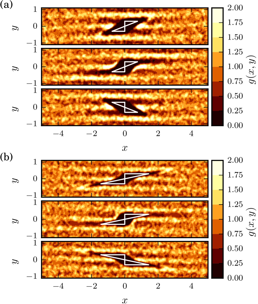
Figure 14: (Color online) The 2-dimensional correlation function $g(x,y)$ at high shear rates over half a period at (a) $\Gamma_{\mathrm{s}}=16.0$ and (b) $\Gamma_{\mathrm{s}}=30.0$. Colors indicate the particle density. At the white patches, $g(x,y)$ exceeds $2.0$. Each sub-figure shows, from top to bottom, snapshots at $t=0$, $t=T/4$, and $T=T/2$. We observe a break-down of the mirror symmetry found at lower shear rates. While the free space is tilted to the right at the beginning of a period, half a period later it is tilted to the opposite direction. Moreover, we find remnants of the hexagonal lattice in the form of stripes of increased density spaced by roughly the layer distance of the crystal. The white triangles indicate how far the populated rows have been sheared against each other over the past quarter period. They are set at arbitrary height such that features of the correlation function are not occluded. Simulation of 900 particles, $\Gamma_{\mathrm{i}}=0.1$

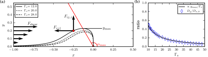
Figure 15: Formation of a shear rate dependent depletion zone (a) and ratio of the bare diffusivities and length scales in dependence on the shear rate (b). In (a), we consider two particles ($\bullet$$\circ$), one being fixed at the origin, and the other one being subject to the forces (arrows) due to particle interaction $\mathbf{F}_{ij}$ at $\Gamma_{\mathrm{i}}=0.1$ and the shear $\mathbf{F}_{\mathrm{shear}}$, which linearly increases with the separation in the $y$-direction. Black lines represent the points where horizontal forces are balanced. Below, the free particle moves to the left, i.e. particles outside the area cannot enter it. With increasing shear rate, the maximum value $y_{\max}$ decreases. The red line marks the position of largest thickness of the depletion zone, changing with $\Gamma_{\mathrm{s}}$. In (b), the ratio of the bare diffusivities $D_{y}/D_{x,0}$ shows the same behavior as the quotient $y_{\max{}}/\Gamma_{\mathrm{s}}$.

The picture changes upon advancing to higher shear rates. In Fig. 14 are shown the 2d correlations $g(x,y)$ across half a period at $\Gamma_{\mathrm{s}}=16.0$ and $30.0$, respectively. In figure (a) are shown snapshots of $\Gamma_{\mathrm{s}}=16.0$ at the beginning of a period, at the turning point of $t=T/4$ when the flow has stopped and strain is maximal, and after half a period at $t=T/2$, when the flow has reversed its direction and strain is zero again. The most prominent feature is the break-down of the symmetry. At the start of the period, $t=0$, we observe a dark brown rhombic region around the origin where no other particles are found. It is oriented to the right. As would be expected from the symmetry of the flow, half a period later we observe a similar rhombus, but this time oriented to the left. In between, at the turning point of the flow, its outer boundary at $y\approx\pm 0.5$ is stretched along the strain even more, while at the centerline $y=0$ it keeps its boundaries. In effect, this leads to less populated protrusions above and below the centerline, concurrent with the relative strain. They closely resemble the gaps found in models describing the emergence of moonlet propellers in Saturn’s A ring Spahn and Sremcevic (2000); *Sremcevic2002; *Sremcevic2007. A ‘propeller-shaped’ region was also described by Keim et al. (2013) in their study of the model in Corté et al. (2008). Due to a different definition of the shear protocol, our snapshot at $t=T/4$ corresponds to $t=T/2$ in their system, and by symmetry relates to $t=T$. A remarkable difference to their observation is that they describe the correlations for the reversible state, whereas we here find it in the irreversible state. Therefore, also the irregular state maintains a phase memory of the shear process, at least for the interactions studied here.

We can understand this phenomenon when starting at $t=-T/4$. At this time, the flow is at its left turning point. We now look at the line $x=0$. At short distances, particles on the left of this line are repelled to the left, and over the next quarter period, the flow is not fast (i.e. strong) enough to pull them beyond $x=0$. Thus, at $t=0$ we observe the rhombus: it simply corresponds to the line $x=0$, advected over the last quarter period. This suppression of transport continues up to $t=T/4$. Since this does not apply to the centerline, the rhombic shape gets distorted and we observe the aforementioned protrusions. As soon as the low density area leaves the core area, particles from the other sides are pushed into the void. This is reflected by a slight increase in $g(x,y)$ towards the tips of the protrusions. However, at $t=T/2$, the remnants are still visible (brown (gray) areas in the upper right and lower left).

The maxima of the correlation function are found at $x\approx\pm 1.0$ and $y=0$ at every time step. This corresponds to a strong localization of next neighbors parallel to the shear. Additionally, in the perpendicular direction we find a modulation in particle density, with maxima at $y\approx 0$ and $\pm 0.6\dots 0.8$, and multiples thereof. The modulations extent over several particle distances parallel to the shear before they become weaker and decay. This has two implications. First, although the system is far from its equilibrium of a hexagonal lattice configuration, it still shows the vertical density modulation corresponding to the layers in the lattice. With increasing shear rate, this becomes less pronounced, but is still detectable. Second, those maxima in the correlation function hint at a general anisotropy: The next neighbor distance parallel to the shear is conspicuously larger than the next neighbor distance in the perpendicular direction, as reflected in the location of the layers.

At the higher shear rate $\Gamma_{\mathrm{s}}=30.0$, shown in Fig. 14(b), the picture qualitatively stays the same. We still observe the density modulations and the flow dependent variation of the next neighbor distances. What changes is the shape of the particle-free space. At the beginning of the period, it gets stretched even more, but does not resemble a rhombus any more. This is due to the fixed neighbor relations along the centerline at $x\approx\pm 0.8\dots 1.2$. At the turning point, $t=T/4$, the free space is a slightly tilted oval instead of a rounded rhombus. As expected, the density modulations in the perpendicular direction have a smaller wavelength than at $\Gamma_{\mathrm{s}}=16.0$, and the first maxima are found at $y\approx\pm 0.5\dots 0.6$.

The reduction of the vertical spacing with shear rate can be explained within a simple model. To this end, we consider two particles, a fixed one placed at the origin and a free one, as sketched in Fig. 15(a). For now, we replace the periodic shear by a constant one which linearly increases with the separation $y$. Thus, the free particle is subject to two different forces, the inter-particle force $\mathbf{F}_{ij}$ and the shear force $\mathbf{F}_{\mathrm{shear}}$ acting along the $x$-direction. Taking only forces parallel to the shear into account, we can compute the particle position where horizontal forces balance,

$$F_{\mathrm{shear}} =-F_{ij,\parallel}.$$ (24)

If the mobile particle is close to the $x$-axis, forces are balanced at large distances. For larger separations in $y$, the shear force dominates and the force from the stationary particle is too weak to balance them. The curves of horizontal force equilibrium are shown in Fig. 15(a) for various shear rates. Particles in the area below the curves move to the left and are deflected upwards until they are finally far enough away to pass the stationary particle. This deflection can also be observed in the correlation function in Fig. 14 at $t=T/4$, where the maximum at $x=\pm 1$ is bent away from the centerline. Due to the periodic repetition and the many-particle interactions, this eventually leads to the formation of a somewhat larger depletion zone where $g(x,y)$ is very low. When increasing the shear rate, forces are balanced closer to the origin and so the area of the depletion zone decreases. The maximum separation $y_{\max}$ varies along a straight line with $\alpha_{\max}=2\pi/3$ the angle towards the $x$-axis, and approaches the origin in the limit of very large shear rates. By contrast, the hard-core interactions used by Keim et al. (2013) do not lead to a shear rate dependent separation: They report a constant separation in the perpendicular direction with boundaries at $y=\pm 1$.

Advection-diffusion coupling (14) is based upon the assumption that a single particle performs diffusive motion. However, in the system studied in this paper we have a multi-particle interaction and thus the effects of the surrounding particles have to be taken into account. These interactions determine the anisotropies of the diffusivities in Fig. 7. To see this, note that the free path of a particle is determined by the regions of low particle density, i.e. low $g(x,y)$. From the previous observations and the simple model, we can derive two assumptions: First, the free path perpendicular to the shear is governed by the maximum separation $y_{\max}$. Obviously, they do not correspond directly to each other since $y_{\max}$ is smaller than the separation in Fig. 14. Yet, $y_{\max}$ should determine the general dependency on the shear rate. Second, the free path parallel to the shear is set by the low-density protrusions, which roughly increase along with the shear rate $\Gamma_{\mathrm{s}}$.

These assumptions then suggest that the ratio of the bare diffusivities $D_{y}/D_{x,0}$ should be proportional to $y_{\max{}}/\Gamma_{\mathrm{s}}$. Fig. 15(b) shows that this is indeed the case for $\Gamma_{\mathrm{s}}>15$. This shows that the unexpected anisotropy of the system is connected with the emergence of two different length scales which change with the shear rate.

VI Summary

We have seen that even a model as simple as (6) displays features usually associated with much more complex systems. We found chaotic and ordered behavior which can occur in different regions of the parameter space $(\Gamma_{\mathrm{i}},\Gamma_{\mathrm{s}})$: The transition is similar for each value of the interaction strength: For small shear strains, after some transient time the system becomes reversible, the shear can be considered as a small perturbation. Beyond an interaction-dependent critical shear rate, this feature is lost and we observe chaotic motion. For stronger interactions, the critical point is delayed to higher shear rates.

We identified the diffusivity as an indicator of chaotic motion. As would be expected for a diffusive system subject to shear, we observe advection-diffusion coupling: The parallel diffusivity is strongly enhanced as compared to perpendicular diffusivity. For large interaction strengths, we can explain this anisotropy using eqn. (14). For low interactions though we observe additional anisotropic effects, which we can attribute to the 2d-correlations of particles: Whereas the free space parallel to the shear increases with the shear rate, the next neighbor distance perpendicular to the shear decreases with increasing shear rate. Both effects combined allow us to explain the relative anisotropy of the bare diffusivities. Additionally, we were able to identify a phase dependency of the particle distributions, which is concealed when looking upon e.g. stroboscopic maps.

Finally, we could relate the critical shear rate associated with the loss of reversibility to the stability properties of sheared regular lattices. So at least for the present system the onset of irreversibility is connected with an instability of the asymptotic, regular state.

References

- Hahn (1950) E. L. Hahn, Phys. Rev. 80, 580 (1950).
- Carr and Purcell (1954) H. Y. Carr and E. M. Purcell, Phys. Rev. 94, 630 (1954).
- Homsy (2008) G. M. Homsy, ed., Multimedia Fluid Dynamics, 2nd ed. (Cambridge University Press, 2008).
- Niggemeier et al. (1993) W. Niggemeier, G. von Plessen, S. Sauter, and P. Thomas, Phys. Rev. Lett. 71, 770 (1993).
- Chaiken et al. (1986) J. Chaiken, R. Chevray, M. Tabor, and Q. M. Tan, Proc. R. Soc. A 408, 165 (1986).
- Roberts and Quispel (1992) J. A. G. Roberts and G. R. W. Quispel, Phys. Rep. 216, 63 (1992).
- Casati et al. (1986) G. Casati, B. V. Chirikov, I. Guarneri, and D. L. Shepelyansky, Phys. Rev. Lett. 56, 2437 (1986).
- Pastawski et al. (1995) H. M. Pastawski, P. R. Levstein, and G. Usaj, Phys. Rev. Lett. 75, 4310 (1995).
- Eckhardt (2003) B. Eckhardt, J. Phys. A 36, 371 (2003).
- Pine et al. (2005) D. J. Pine, J. P. Gollub, J. F. Brady, and A. M. Leshansky, Nature 438, 997 (2005).
- Guasto et al. (2010) J. S. Guasto, A. S. Ross, and J. P. Gollub, Phys. Rev. E 81, 061401 (2010).
- Metzger and Butler (2012) B. Metzger and J. E. Butler, Phys. Fluids 24, 021703 (2012).
- Jeanneret and Bartolo (2014) R. Jeanneret and D. Bartolo, Nat. Commun. 5, 3474 (2014).
- Franceschini et al. (2011) A. Franceschini, E. Filippidi, E. Guazzelli, and D. J. Pine, Phys. Rev. Lett. 107, 250603 (2011).
- Franceschini et al. (2014) A. Franceschini, E. Filippidi, E. Guazzelli, and D. J. Pine, Soft Matter 10, 6722 (2014).
- Keim and Arratia (2013) N. C. Keim and P. E. Arratia, Soft Matter 9, 6222 (2013).
- Keim and Arratia (2014) N. C. Keim and P. E. Arratia, Phys. Rev. Lett. 112, 028302 (2014).
- Metzger and Butler (2010) B. Metzger and J. E. Butler, Phys. Rev. E 82, 051406 (2010).
- Düring et al. (2009) G. Düring, D. Bartolo, and J. Kurchan, Phys. Rev. E 79, 030101 (2009).
- Corté et al. (2008) L. Corté, P. M. Chaikin, J. P. Gollub, and D. J. Pine, Nat. Phys. 4, 420 (2008).
- Corté et al. (2009) L. Corté, S. J. Gerbode, W. Man, and D. J. Pine, Phys. Rev. Lett. 103, 248301 (2009).
- Menon and Ramaswamy (2009) G. I. Menon and S. Ramaswamy, Phys. Rev. E 79, 061108 (2009).
- Keim and Nagel (2011) N. C. Keim and S. R. Nagel, Phys. Rev. Lett. 107, 010603 (2011).
- Mohan et al. (2013) L. Mohan, C. Pellet, M. Cloitre, and R. Bonnecaze, J. Rheol. 57, 1023 (2013).
- Regev et al. (2013) I. Regev, T. Lookman, and C. Reichhardt, Phys. Rev. E 88, 062401 (2013).
- Fiocco et al. (2013) D. Fiocco, G. Foffi, and S. Sastry, Phys. Rev. E 88, 020301 (2013).
- Fiocco et al. (2014) D. Fiocco, G. Foffi, and S. Sastry, Phys. Rev. Lett. 112, 025702 (2014).
- Slotterback et al. (2012) S. Slotterback, M. Mailman, K. Ronaszegi, M. van Hecke, M. Girvan, and W. Losert, Phys. Rev. E 85, 021309 (2012).
- Schreck et al. (2013) C. F. Schreck, R. S. Hoy, M. D. Shattuck, and C. S. O’Hern, Phys. Rev. E 88, 052205 (2013).
- Royer and Chaikin (2014) J. R. Royer and P. M. Chaikin, Proc. Natl. Acad. Sci. 112, 49 (2014).
- Mangan et al. (2008) N. Mangan, C. Reichhardt, and C. J. Olson Reichhardt, Phys. Rev. Lett. 100, 187002 (2008).
- Zhang et al. (2010) W. Zhang, W. Zhou, and M. Luo, Phys. Lett. A 374, 3666 (2010).
- Okuma et al. (2010) S. Okuma, Y. Suzuki, and Y. Tsugawa, Phys. C 470, S842 (2010).
- Motohashi and Okuma (2011) A. Motohashi and S. Okuma, J. Phys. Conf. Ser. 302, 012029 (2011).
- Okuma et al. (2011) S. Okuma, Y. Tsugawa, and A. Motohashi, Phys. Rev. B 83, 012503 (2011).
- Melzer et al. (1996a) A. Melzer, A. Homann, and A. Piel, Phys. Rev. E 53, 2757 (1996a).
- Melzer et al. (1996b) A. Melzer, V. A. Schweigert, I. V. Schweigert, A. Homann, S. Peters, and A. Piel, Phys. Rev. E 54, R46 (1996b).
- Schweigert et al. (1998) V. A. Schweigert, I. V. Schweigert, A. Melzer, A. Homann, and A. Piel, Phys. Rev. Lett. 80, 5345 (1998).
- Lees and Edwards (1972) A. W. Lees and S. F. Edwards, J. Phys. C: Solid State Phys. 5, 1921 (1972).
- Note (1) See Supplemental Material at URL for movies.
- Young et al. (1982) W. R. Young, P. B. Rhines, and C. J. R. Garrett, J. Phys. Oceanogr. 12, 515 (1982).
- Chicone (2006) C. Chicone, Ordinary Differential Equations with Applications, Texts in Applied Mathematics, Vol. 34 (Springer New York, 2006).
- Spahn and Sremcevic (2000) F. Spahn and M. Sremcevic, Astron. Astrophys. 358, 368 (2000).
- Sremcevic et al. (2002) M. Sremcevic, F. Spahn, and W. J. Duschl, Mon. Not. R. Astron. Soc. 337, 1139 (2002).
- Sremcević et al. (2007) M. Sremcević, J. Schmidt, H. Salo, M. Seiss, F. Spahn, and N. Albers, Nature 449, 1019 (2007).
- Keim et al. (2013) N. C. Keim, J. D. Paulsen, and S. R. Nagel, Phys. Rev. E 88, 032306 (2013).