$c$-function and central charge of the sine-Gordon model from the non-perturbative renormalization group flow

Abstract

In this paper we study the $c$-function of the sine-Gordon model taking explicitly into account the periodicity of the interaction potential. The integration of the $c$-function along trajectories of the non-perturbative renormalization group flow gives access to the central charges of the model in the fixed points. The results at vanishing frequency $\beta^{2}$, where the periodicity does not play a role, are retrieved and the independence on the cutoff regulator for small frequencies is discussed. Our findings show that the central charge obtained integrating the trajectories starting from the repulsive low-frequencies fixed points ($\beta^{2}<8\pi$) to the infrared limit is in good quantitative agreement with the expected $\Delta c=1$ result. The behavior of the $c$-function in the other parts of the flow diagram is also discussed. Finally, we point out that also including higher harmonics in the renormalization group treatment at the level of local potential approximation is not sufficient to give reasonable results, even if the periodicity is taken into account. Rather, incorporating the wave-function renormalization (i. e. going beyond local potential approximation) is crucial to get sensible results even when a single frequency is used.

I Introduction

Statistical field theory has known an outpouring development in the last decades, with the systematic improvement of powerful theoretical tools for the study of critical phenomena and phase transitions giuseppe . A key role among these methods is played by the renormalization group (RG) approach: RG allowed to treat statistical physics models studying the behavior of the transformations bringing the microscopic variables into macroscopic ones Goldenfeld ; Cardy . Using RG one can have not only a qualitative picture of the phase diagram and fixed points, but also accurate quantitative estimates of critical properties as critical exponents and universal quantities - even though very few cases are known where RG procedure can be carried out exactly and the method itself offers few possibility to obtain exact results.

On the other hand, the scale invariance exhibited by systems at criticality may give rise to invariance under the larger group of conformal transformations polyakov_1970 locally acting as scale transformations di_francesco_1997 . The conformal group in $d$ spatial dimensions (for $d\neq 2$) has a number of independent generators equal to $\frac{1}{2}(d+1)(d+2)$, while for $d=2$ the conformal group is infinitely dimensional di_francesco_1997 . The occurrence and consequences of conformal invariance for $2$-dimensional field theories have been deeply investigated and exploited to obtain a variety of exact results di_francesco_1997 ; giuseppe and a systematic understanding of phase transitions in two dimensions.

A bridge between conformal field theory (CFT) techniques and the RG description of field theories is provided in two dimensions by the $c$-theorem. Far from fixed points, Zamolodchikov’s $c$-theorem c_theorem can be used to get information on the scale-dependence of the model. In particular the theorem states that it is always possible to construct a function of the couplings, the so-called $c$-function, which monotonically decreases when evaluated along the trajectory of the RG flow. Furthermore, at the fixed points this function assumes the same value as the central charge of the corresponding CFT giuseppe .

Although the $c$-theorem is by now a classical result, the determination of the $c$-function is not straightforward and its computation far from fixed points is non-trivial even for very well known models, so that methods as form factor perturbation theory, truncated conformal space approach and conformal perturbation theory has been developed giuseppe . In $d=2$ an expression of the $c$-function has been obtained in the framework of form factor perturbation theory cardy_prl for theories away from criticality and it has been applied to the sinh-Gordon model fring . The sinh-Gordon model is a massive integrable scalar theory, with no phase transitions. In fring one finds $\Delta c=1$ for the sinh-Gordon theory. In a recent result dorey , the analytical continuation of the sinh-Gordon $S$-matrix produces a roaming phenomenon exhibiting $\Delta c=1$ and multiple plateaus of the $c$-function. The analytic continuation $\beta\to i\beta$ of the sinh-Gordon model leads to the well-known sine-Gordon (SG) model with a periodic self interaction of the form $\cos{(\beta\phi)}$.

The SG model presents the unique feature to have a whole line of interacting fixed points with coupling (temperature) dependent critical exponents. It is in the same universality of the $2$-dimensional Coulomb gas minnaghen and of the $2$-dimensional $XY$ kadanoff , thus being one of the most relevant and studied $2$-dimensional model, with applications ranging from the study of the Kosterlitz-Thouless transition kadanoff to quantum integrability korepin and bosonization tsvelik . In particular, for the SG model an ubiquitous issue is how to deal with the issue of the periodicity of the field coleman , which unveils and plays a crucial role for $\beta\neq 0$. Given the importance of the SG as a paradigmatic $2$-dimensional model, the determination of the $c$-function from the non-perturbative RG flow is a challenging goal, in particular to clarify the role played by the periodicity of the field for $\beta\neq 0$.

From the RG point of view, the determination of the behavior of the $c$-function is a challenging task requiring a general non-perturbative knowledge of the RG flow. Recently c_func , an expression for the Zamolodchikov’s $c$-function has been derived for $2$-dimensional models in the Functional RG (FRG) framework Berges02 ; Polony04 ; Delamotte12 : resorting to an approximation well established and studied in the FRG, the Local Potential Approximation (LPA), an approximated and concretely computable RG flow equation for the $c$-function was also written down c_func . By using this expression known results were recovered for scalar models on some special trajectories of the Ising and SG models. For the SG model, having a Lagrangian proportional to $\cos{(\beta\phi)}$, the determination and the integration of the $c$-function was carried out for $\beta=0$ as a massive deformation of the Gaussian fixed point c_func . Motivated by these results, both for the Ising and SG models and for general $2$-dimensional models, it would be highly desirable to have a complete description of the $c$-function on general RG trajectories.

In the present paper we present the first numerical calculation of the $c$-function on the whole RG flow phase diagram of the SG model. The goal is to determine the behavior of the $c$-function, and the presence of known results (namely, $\Delta c=1$) helps to assess the validity of our approach along the different flows. We also complete the description initiated in c_func moving to more complex trajectories and showing that these cases are not a straightforward generalization of the known results. We finally discuss the dependence of these results on the approximation scheme used to compute FRG equations.

II Functional Renormalization Group Method

In this section, we briefly summarize the FRG approach Berges02 ; Polony04 ; Delamotte12 . Starting from the usual concepts of Wilson’s renormalization group (RG) it is possible to derive an exact flow equation for the effective action of any quantum field theory. T his flow equation is commonly written in the form

$$k\partial_{k}\Gamma_{k}[\varphi]=\frac{1}{2}\mathrm{Tr}\left[\frac{k\partial_{k}R_{k}}{\Gamma^{(2)}_{k}[\varphi]+R_{k}}\right],$$ (1)

where $\Gamma_{k}[\varphi]$ is the effective action and $\Gamma^{(2)}_{k}[\varphi]$ denotes the second functional derivative of the effective action. The trace Tr stands for an integration over all the degrees of freedom of the field $\phi$, while $R_{k}$ is a regulator function depending on the mode of the field and on the running scale $k$. When the running scale goes to zero $k\to 0$ the scale-dependent effective action $\Gamma_{k=0}[\phi]$ is the exact effective action of the considered quantum field theory.

Usually equation (1) is treated in momentum space, thus the trace stands for a momentum integration and the regulator $R_{k}$ is a smooth function which freezes all the modes with momentum smaller than the scale $k$.

The exact FRG equation (1) stands for functionals, thus it is handled by truncations. Truncated RG flows depend on the choice of the regulator function $R_{k}$, i.e. on the renormalization scheme. Regulator functions have already been discussed in the literature by introducing their dimensionless form

$$R_{k}(p)=p^{2}r(y),\hskip 14.22636pty=p^{2}/k^{2},$$ (2)

where $r(y)$ is dimensionless. Various types of regulator functions can be chosen (an archetype of regulator functions css has been shown to take the forms of the regulators used so far by setting its parameters). In this work we are going to consider the following regulators

$$r_{{\mathrm{pow}}}(y)=\frac{1}{y^{b}},$$ (3a)

$$r_{{\mathrm{opt}}}(y)=\left(\frac{1}{y}-1\right)\theta(1-y),$$ (3b)

where the first is known as the power-law type Mo1994 and the second one is the Litim (or optimized) opt_rg type regulator. Let us note that the so called mass cutoff regulator, which is used in c_func , is identical to $r_{{\mathrm{pow}}}(y)$ with $b=1$.

One of the commonly used systematic approximations is the truncated derivative expansion, where the action is expanded in powers of the derivative of the field Berges02 :

$$\Gamma_{k}[\varphi]=\int_{x}\left[V_{k}(\varphi)+Z_{k}(\varphi)\frac{1}{2}(\partial_{\mu}\varphi)^{2}+\cdots\right].$$

In LPA higher derivative terms are neglected and the wave-function renormalization is set equal to constant, i.e. $Z_{k}\equiv 1$. In this case (1) reduces to the partial differential equation for the dimensionless blocked potential ($\tilde{V}_{k}=k^{-2}V_{k}$) which has the following form in 2 dimensions

$$(2+k\partial_{k}){\tilde{V}}_{k}(\varphi)=-\frac{1}{4\pi}\int_{0}^{\infty}dy\frac{y^{2}\frac{dr}{dy}}{(1+r)y+{\tilde{V}^{\prime\prime}}_{k}(\varphi)}.$$ (4)

III The $c$-function in the Framework of Functional Renormalization Group

An expression for the $c$-function in FRG was recently developed in c_func . In this section we are going to give the guidelines of this derivation, reviewing the main results used in the next sections.

Let us start considering an effective action $\Gamma[\phi,g]$ for a single field $\phi$ in curved space, with metric $g_{\mu\nu}$. We can study the behavior of this effective action under transformation of the field and the metric:

$$\phi\rightarrow e^{d_{\phi}\tau}\phi$$ (5)

$$g_{\mu\nu}\rightarrow e^{2\tau}g_{\mu\nu}$$ (6)

where $d_{\phi}$ is the conformal weight of the field ($d_{\phi}=-\frac{d-2+\eta}{2}$ for a scalar field) while the background metric $g_{\mu\nu}$ has always conformal weight $2$. From the requirement that the effective action must be invariant under the Weyl transformation (5)-(6), we obtain the following expression for a conformal field theory (CFT) in curved space c_func ,

$$\Gamma[\phi,g]=S_{CFT}[\phi,g]+cS_{P}[g].$$ (7)

$S_{CFT}[\phi,g]$ is the curved space generalization of the standard CFT action, which is recovered in the flat space case $g_{\mu\nu}=\delta_{\mu\nu}$, $c$ is the central charge of our theory and $S_{P}[g]$ is the Polyakov action term which is necessary to maintain the Weyl invariance of the effective average action in curved space.

To obtain FRG equations one has to add an infra-red (IR) cutoff term $\Delta S_{k}[\phi,g]$ to the ultra-violet (UV) action of the theory. This is a mass term which depends both on the momentum of the excitations and on a cutoff scale $k$.

$$\Delta S_{k}[\phi,g]=\frac{1}{2}\int{d^{2}x\sqrt{g}\phi(x)R_{k}(\Delta)\phi(x)},$$ (8)

where $\Delta$ is the spatial Laplacian operator. The effect is to freeze the excitation of momentum $q\ll k$, but leaving the excitation at $q>k$ almost untouched. The result of this modification of the UV action is to generate, after integrating over the field variable, a scale-dependent effective action $\Gamma_{k}[\phi,g]$ which describes our theory at scale $k$. When the scale $k$ is sent to zero the cutoff term in the UV action vanishes and the $\Gamma_{k}[\phi,g]$ is the exact effective average action of the theory.

The generalization of (7) in presence of the cutoff terms is

$$\Gamma_{k}[\phi,g]=S_{k}[\phi,g]+c_{k}S_{P}[g]+\cdots,$$ (9)

where $c_{k}$ is now the scale-dependent $c$-function and the dots stands from some geometrical terms which do not depend on the field. We should now consider the case of a flat metric with a dilaton background $g_{\mu\nu}=e^{2\tau}\delta_{\mu\nu}$. Using the standard path integral formalism for the effective action we can write

$$\begin{split}&e^{-\Gamma_{k}[\phi,e^{2\tau}\delta]}=e^{-S_{k}[\phi,e^{2\tau}\delta]-c_{k}S_{P}[e^{2\tau}\delta]}=\\ &\int{\mathcal{D}\chi_{d.b.}e^{-S_{UV}[\phi+\chi,e^{2\tau}\delta]-c_{UV}S_{P}[e^{2\tau}\delta]-\Delta S_{k}[\chi,e^{2\tau}\delta]}}\end{split}$$ (10)

where $S_{UV}[\phi,g]$ is some UV action, $c_{UV}$ is the value of the $c$-function in the UV (which can be equal to the central charge of some CFT if we are starting the flow from a conformal invariant theory) and $\chi$ is the fluctuation field. The notation $\mathcal{D}\chi_{d.b.}$ stands for an integration over the fluctuation field $\chi$ in the curved space of the dilaton background c_func . We can further manipulate latter expression moving $c_{UV}$ on the l.h.s

$$\begin{split}&e^{-S_{k}[\phi,e^{2\tau}\delta]+(c_{UV}-c_{k})S_{P}[e^{2\tau}\delta]}=\\ &\int{\mathcal{D}\chi_{d.b.}e^{-S_{UV}[\phi+\chi,e^{2\tau}\delta]-\Delta S_{k}[\chi,e^{2\tau}\delta]}}.\end{split}$$ (11)

The Polyakov action in the dilaton background case assumes the form

$$S_{P}[g]=-\frac{1}{24}\int{\tau\Delta\tau},$$ (12)

where $\tau$ is the dilaton field, $\Delta$ is the laplacian operator and the integral is over an implicit spatial variable. Substituting latter expression into (11) we obtain

$$\begin{split}&e^{-S_{k}[\phi,e^{2\tau}\delta]-\frac{(c_{UV}-c_{k})}{24}\int\tau\Delta\tau}=\\ &\int{\mathcal{D}\chi_{d.b.}e^{-S_{UV}[\phi+\chi,e^{2\tau}\delta]-\Delta S_{k}[\chi,e^{2\tau}\delta]}}.\end{split}$$ (13)

In order to recover the usual flat metric integration we have to pursue a Weyl transformation (5) for the fields $\phi$ and $\chi$

$$\begin{split}&e^{-S_{k}[e^{d_{\phi}\tau}\phi,e^{2\tau}\delta]-\frac{(c_{UV}-c_{k})}{24}\int\tau\Delta\tau}=\\ &\int{\mathcal{D}\chi e^{-S_{UV}[e^{d_{\phi}\tau}(\phi+\chi),e^{2\tau}\delta]-\Delta S_{k}[e^{d_{\phi}\tau}\chi,e^{2\tau}\delta]}},\end{split}$$ (14)

and now the integration measure is in flat space.

Finally deriving previous expression with respect to the logarithm of the FRG scale we obtain that the flow of the $c$-function $\partial_{t}c_{k}$ can be extracted from the flow of the cutoff action (8) by taking the coefficient of the $\int\tau\Delta\tau$ term,

$$k\partial_{k}c_{k}=24\pi\langle k\tilde{\partial}_{k}\Delta S_{k}[e^{d_{\phi}\tau}\chi,e^{2\tau}\delta]\rangle\Bigl{|}_{\int{\tau\Delta\tau}},$$ (15)

which after some manipulation becomes c_func

$$k\partial_{k}c_{k}=-12\pi k\tilde{\partial}_{k}G_{k}[\tau]\Bigl{|}_{\int{\tau\Delta\tau}}.$$ (16)

Eq. (16) shows that the $c$-function flow is proportional to the coefficient of the $\int{\tau\Delta\tau}$ term in the expansion of the propagator flow $k\tilde{\partial}_{k}G_{k}[\tau]$, also this flow has to be computed taking into account only the $k$ dependence of the regulator function, i.e.

$$k\tilde{\partial}_{k}=k\partial_{k}R_{k}\frac{\partial}{\partial R_{k}}.$$ (17)

This equation describes the exact flow of the $c$-function into the FRG framework.

Since it is not in general possible to solve exactly equation (1) and also equation (16) needs to be projected into a simplified theory space to be computed numerically. In Ref. c_func an explicit expression for the flow equation of the $c$-function in the LPA scheme has been derived with the mass cutoff

$$k\partial_{k}c_{k}=\frac{[k\partial_{k}\tilde{V}^{\prime\prime}_{k}(\varphi_{0,k})]^{2}}{[1+\tilde{V}^{\prime\prime}_{k}(\varphi_{0,k})]^{3}},$$ (18)

with the dimensionless blocked potential $\tilde{V}_{k}(\varphi)$ which is evaluated at its running minimum $\varphi=\varphi_{0,k}$ (i.e. the solution of $\tilde{V}^{\prime}_{k}(\varphi)=0$). We observe that an explicit expression for the $c$-function beyond LPA is not available in literature.

It should be noticed that, while (4) is valid for any regulator (cutoff) function, the expression for the $c$-function (18) has been obtained by using the mass cutoff, i.e. (3a) with $b=1$. Other cutoff choices proved to be apparently very difficult to investigate. In the following, we will argue that while the expression (18) is sufficient to obtain a qualitative (and almost quantitative) picture of the $c$-function phase diagram the usage of other regulator functions is necessary to achieve full consistency. Where it is possible we will check the cutoff dependence of our numerical results.

IV RG study of the sine-Gordon model

The SG scalar field theory is defined by the Euclidean action for $d=2$

$$\Gamma_{k}[\phi]=\int d^{2}x\left[\frac{1}{2}(\partial_{\mu}\varphi_{x})^{2}-u\cos(\beta\varphi_{x})\right],$$ (19)

where $\beta$ and $u$ are the dimensional couplings. Since we are interested in the FRG study of the SG model which is periodic in the field variable, the symmetry of the action under the transformation nandori_sg

$$\varphi(x)\to\varphi(x)+{\cal A}$$ (20)

is to be preserved by the blocking and the potential $\tilde{V}_{k}(\varphi)$ must be periodic with period length ${\cal A}$. It is actually obvious that the blocking, i.e. the transformation given by replacing the derivative with respect to the scale $k$ by a finite difference in (4) preserves the periodicity of the potential nandori_sg ; schemes .

IV.1 The FRG equation for the SG model for scale-independent frequency.

In LPA one should look for the solution of (4) among the periodic function which requires the use of a Fourier expansion. When considering a single Fourier mode, the scale-dependent blocked potential reads

$$\tilde{V}_{k}(\varphi)=-\tilde{u}_{k}\cos(\beta\varphi),$$ (21)

where $\beta$ is scale-independent.

In the mass cutoff case, i.e. the power law regulator (3a) with $b=1$, one can derive nandori_msg the flow equation for the Fourier amplitude of (21) from Eq. (4):

$$(2+k\partial_{k})\tilde{u}_{k}=\frac{1}{2\pi\beta^{2}\tilde{u}_{k}}\left[1-\sqrt{1-\beta^{4}\tilde{u}^{2}_{k}}\right]$$ (22)

(see Eq. (21) of nandori_msg for vanishing mass). Similarly, using the optimized regulator (3b) gives

$$(2+k\partial_{k})\tilde{u}_{k}=\frac{1}{2\pi\beta^{2}\tilde{u}_{k}}\left[\frac{1}{\sqrt{1-\beta^{4}\tilde{u}^{2}_{k}}}-1\right].$$ (23)

IV.2 The FRG equation for the SG model for scale-dependent frequency.

A very simple, but still sensible, modification to ansatz (19) is the inclusion of a scale dependent frequency, which, in order to explicitly preserve periodicity, should be rather considered as a running wave-function renormalization. The ansatz then becomes

$$\Gamma_{k}=\int d^{2}x\left[\frac{1}{2}z_{k}(\partial_{\mu}\varphi_{x})^{2}+V_{k}(\varphi_{x})\right],$$ (24)

where the local potential contains a single Fourier mode

$$V_{k}(\varphi)=-u_{k}\cos(\varphi),$$ (25)

and the following notation has been introduced

$$z_{k}\equiv 1/\beta_{k}^{2}$$ (26)

via the rescaling of the field $\varphi\to\varphi/\beta_{k}$ in (19), where $z_{k}$ plays the role of a field-independent wave-function renormalization. Then Eq. (1) leads to the evolution equations

$$k\partial_{k}V_{k}=\frac{1}{2}\int_{p}{\cal D}_{k}k\partial_{k}R_{k},$$ (27)

$$k\partial_{k}z_{k}={\cal P}_{0}V^{\prime\prime\prime 2}_{k}\int_{p}{\cal D}_{k}^{2}k\partial_{k}R_{k}\left(\frac{\partial^{2}{\cal D}_{k}}{\partial p^{2}\partial p^{2}}p^{2}+\frac{\partial{\cal D}_{k}}{\partial p^{2}}\right)$$ (28)

with ${\cal D}_{k}=1/(z_{k}p^{2}+R_{k}+V^{\prime\prime}_{k})$ and ${\cal P}_{0}=(2\pi)^{-1}\int_{0}^{2\pi}d\varphi$ is the projection onto the field-independent subspace. The scale $k$ covers the momentum interval from the UV cutoff $\Lambda$ to zero. It is important to stress that Eqs. (27)-(28) are directly obtained using power-law cutoff functions. One may expect that these equations continue to be valid for a general cutoff provided that $R_{k}\to z_{k}R_{k}$ Berges02 . This substitution has been tested for $O(N)$ models, but its validity has been not yet discussed in the literature for the SG model.

Inserting the ansatz (25) into Eqs. (27) and (28) the RG flow equations for the coupling constants can be written as SG_Trun

$$k\partial_{k}u_{k} = \frac{1}{2\pi}\int_{p}~{}\frac{k\partial_{k}R_{k}}{u_{k}}\left(\frac{P_{k}}{\sqrt{P_{k}^{2}-u_{k}^{2}}}-1\right),$$ (29)

$$k\partial_{k}z_{k} = \frac{1}{2\pi}\int_{p}k\partial_{k}R_{k}\biggl{(}\frac{u_{k}^{2}p^{2}(\partial_{p^{2}}P_{k})^{2}(4P_{k}^{2}+u_{k}^{2})}{4(P_{k}^{2}-u_{k}^{2})^{7/2}}$$ (30)

$$-\frac{u_{k}^{2}P_{k}(\partial_{p^{2}}P_{k}+p^{2}\partial_{p^{2}}^{2}P_{k})}{2(P_{k}^{2}-u_{k}^{2})^{5/2}}\biggr{)}$$

with $P_{k}=z_{k}p^{2}+R_{k}$. In general, the momentum integrals have to be performed numerically, however in some cases analytical results are available. Indeed, by using the power-law regulator (3a) with $b=1$, the momentum integrals can be performed nandori_msg and the RG flow equations read as

$$(2+k\partial_{k}){\tilde{u}}_{k} = \frac{1}{2\pi z_{k}{\tilde{u}}_{k}}\left[1-\sqrt{1-{\tilde{u}}_{k}^{2}}\right]$$

$$k\partial_{k}z_{k} = -\frac{1}{24\pi}\frac{{\tilde{u}}_{k}^{2}}{[1-{\tilde{u}}_{k}^{2}]^{\frac{3}{2}}}$$ (31)

with the dimensionless coupling ${\tilde{u}}=k^{-2}u$. By using the replacements

$$z_{k}\to 1/\beta_{k}^{2},$$ (32a)

$$\tilde{u}_{k}\to\beta_{k}^{2}\tilde{u}_{k},$$ (32b)

and keeping the frequency scale-independent ($\partial_{k}z_{k}=0$ i.e. $\partial_{k}\beta^{2}_{k}=0$) one recovers the corresponding LPA Eq. (22).

V $c$-function of the sine-Gordon model for $\beta=0$

In this section we discuss the case $\beta=0$. We start by summarizing the results obtained for the $c$-function of the SG model in c_func . The ansatz considered in c_func is

$$\tilde{V}_{k}(\varphi)=-\frac{\tilde{m}_{k}^{2}}{\beta_{k}^{2}}\left(\cos(\beta_{k}\varphi)-1\right),$$ (33)

where the frequency $\beta_{k}$ is assumed to be scale-dependent. If one directly substitutes (33) into the RG Eq. (4), then the l.h.s. of (4) generates non-periodic terms due to the scale-dependence of $\beta_{k}$. Thus, the periodicity of the model is not preserved and one can use the Taylor expansion of the original periodic model

$$\tilde{V}_{k}(\varphi)\approx\frac{1}{2}\tilde{m}_{k}^{2}\varphi^{2}-\frac{1}{4!}(\tilde{m}_{k}^{2}\beta_{k}^{2})\varphi^{4}.$$ (34)

In this case, (33) is treated as a truncated Ising model and the RG equations for the coupling constants read as

$$k\partial_{k}\tilde{m}_{k}^{2} = \frac{\tilde{m}_{k}^{2}[\beta_{k}^{2}-8\pi(1+\tilde{m}_{k}^{2})]}{4\pi(1+\tilde{m}_{k}^{2})}$$ (35)

$$k\partial_{k}\beta_{k}^{2} = -\frac{1}{4\pi}\frac{(1+4\tilde{m}_{k}^{2})\beta_{k}^{4}}{(1+\tilde{m}_{k}^{2})^{2}}.$$ (36)

The disadvantage of the scale-dependent frequency is that the periodicity of the model is violated changing the known phase structure of the SG model. However, the authors of c_func were interested in the massive deformation of the Gaussian fixed point which is at $\beta=0$ and $\tilde{u}=0$, so one has to take the limit $\beta\to 0$ where the Taylor expansion represents a good approximation for the original SG model. Indeed, in the limit $\beta\to 0$, the RG Eqs. (35), (36) reduce to

$$k\partial_{k}\tilde{m}_{k}^{2} \approx \frac{\tilde{m}_{k}^{2}[\beta_{k}^{2}-8\pi(1+\tilde{m}_{k}^{2})]}{4\pi(1+\tilde{m}_{k}^{2})}\approx-2\tilde{m}_{k}^{2}$$ (37)

$$k\partial_{k}\beta_{k}^{2} \approx 0.$$ (38)

Similar flow equations for the couplings $\tilde{m}_{k}^{2}$ and $\beta_{k}$ were given in c_func . The solution for the $c$-function based on (33) is in agreement with the known exact result, i.e. at the Gaussian UV fixed point $c_{{\mathrm{UV}}}=1$ and in the IR limit $c_{{\mathrm{IR}}}=0$, thus the exact result in case of the massive deformation of the Gaussian fixed point is $\Delta c=1$ ($\Delta c=c_{UV}-c_{IR}$). The numerical solution c_func gives $\Delta c=0.998$ in almost perfect agreement with the exact result.

Although the numerical result obtained for the $c$-function in c_func is more than satisfactory, due to the Taylor expansion, the SG theory is considered as an Ising-type model. Thus, the RG study of the $c$-function starting from the Gaussian fixed point in the Taylor expanded SG model is essentially the same as that of the deformation of the Ising Gaussian fixed point. So, it does not represent an independent check of (18). Indeed, inserting (37) into (18) using the ansatz (33) one finds

$$k\partial_{k}c_{k}=\frac{4\tilde{m}_{k}^{4}}{[1+\tilde{m}_{k}^{2}]^{3}}$$ (39)

which is identical to Eq. (5.3) of c_func (with $a=1$) obtained for the massive deformation of the Gaussian fixed point in the Ising model and it can be also derived from Eq. (5.19) of c_func in the limit of $\beta^{2}\to 0$.

Therefore, it is a relevant question whether one can reproduce the numerical results obtained for the $c$-function (with the same accuracy) if the SG model is treated with scale-independent frequency (21), or beyond LPA, by the rescaling of the field (25). Also ref. c_func treats only massive deformations of non interacting UV fixed points, then on such trajectories only the mass coupling is running. Nevertheless the c-theorem should hold on all trajectories, even when more couplings are present. Our aim is to demonstrate that the derivation of c_func is valid even in these more general cases, but, due to truncation approach, the approximated FRG phase diagram does not fulfill the requirements of the c-theorem exactly and, therefore, only approximated results are possible.

VI $c$-function of the sine-Gordon model on the whole flow diagram

In this section we study the $c$-function of the SG model on the whole phase diagram, studying both the scale independent wave-function renormalization and the treatment with the running frequency.

VI.1 Scale-independent frequency case

The definition for the SG model used in this work, i.e. (19), differs from (33) because the frequency parameter is assumed to be scale-independent in LPA. The running of $\beta$ can only be achieved beyond LPA by incorporating a wave-function renormalization and using a rescaling of the field variable which gives $z_{k}=1/\beta_{k}^{2}$.

Let us first discuss the results of LPA. Equations (22) and (23) have the same qualitative solution. In Fig. 1 we show the phase structure obtained by solving (23).

Figure 1: The figure shows the phase structure of the SG model obtained by the FRG equation using Litim’s regulator in the scale-independent frequency case. The two phases are separated by $\beta_{c}^{2}=8\pi$. The dashed line shows the line of IR fixed points of the broken phase.

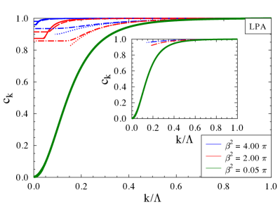
Figure 2: Running of the $c$-function obtained in the scale-independent frequency case by solving (22) (dotted lines - mass cutoff) and (23) (dot-dashed lines - Litim cutoff) combined with (18) for the SG model is plotted for various values of the frequency $\beta^{2}$. From top to bottom it is $\beta^{2}/\pi=4,2,0.005$. Due to the poor convergence properties of (22), where the mass cutoff was used, the RG flow stops at some finite momentum scale and the deep IR value of the $c$-function cannot be reached (dotted lines). The use of the Litim cutoff (23) (dot-dashed lines) can produce us the IR constant for the $c$-function. However, for very small value of $\beta^{2}$ the low-frequency approximation is the best choice, i.e. one has to solve (41) (green line): results from different cutoff functions are indistinguishable. The solid lines represent the results obtained with power law cutoff ($b=2$), while the dashed lines are the results with the exponential cutoff. The inset shows the results for an enlarged theory space where higher harmonics are included in (25) (dot-dashed lines - Litim cutoff).

The RG trajectories are straight lines because in LPA the frequency parameter of (19) is scale independent. Above (below) the critical frequency $\beta^{2}_{c}=8\pi$, the line of IR fixed points is at $\tilde{u}_{{\mathrm{IR}}}=0$ ($\tilde{u}_{{\mathrm{IR}}}\neq 0$). For $\beta^{2}<8\pi$ the IR value for the Fourier amplitude depends on the particular value of $\beta^{2}$ thus, one finds different IR effective theories, i.e. the corresponding CFT depends on the frequency too.

The scaling for the $c$-function is the one expected from the c-theorem. It is a decreasing function of the scale $k$ which is constant in the UV and IR limits, see Fig. 1. Due to the approximation of scale independent frequency $\beta$, here, the IR value of the $c$-function depends on the particular initial condition for $\beta^{2}$. Then when we start at the Gaussian fixed points line ($c=1$), in the symmetric phase, the flow evolves towards an IR fixed point, but at this approximation level, we have different IR fixed points which are all at different $\tilde{u}$ values and consequently the $\Delta c$ values differ from the exact one. The exact result $\Delta c\simeq 1$ is obtained only in the $\beta\to 0$ limit.

We notice that Eq. (22), where the mass cutoff was used, has very poor convergence properties and the flow, obtained from them, stops at some finite scale, thus the deep IR values of the $c$-function cannot be reached (dashed lines in Fig. 2).

The use of the Litim cutoff RG Eq. (23) improves the convergence of the RG flow but the IR results for the $c$-function are very far from the expected $\Delta c=1$, which can be recovered only in the vanishing frequency limit. Also the inclusion of higher harmonics in (25) ( inset in Fig.2) does not improve this result.

It should be noted that Eq. (18) is strictly valid only in the mass cutoff case, however in Fig. 2 we used Eq. (18) even in the optimized cutoff case. This inconsistence cannot be regarded as the cause for the unsatisfactory results obtained in the large $\beta$ cases, indeed we expect very small dependence of the flow trajectories upon the cutoff choice.

This small dependence on the regulator is evident from the comparison of the mass and Litim regulator results of trajectories for the $c$-function in Fig. 2, which are very similar, at least in the region where no convergence problems are found. This similarity justifies the use of the mass cutoff result (18) with RG flow Eqs. (23) obtained by the optimized (Litim) regulator.

We also computed the $c$-function flow for other cutoff functions, namely the power-law $b=2$ (solid lines in Fig. 2) and the exponential one (dashed lines). Apart from the mass cutoff, all the others converge to the IR fixed point. The conclusion is that there is not a pronounced dependence of the findings on the cutoff schemes and that the constant frequency case in not sufficient to recover the correct behavior for the $c$-function.

We observe that the lack of convergence observed in mass cutoff case is not present in the small frequency limit analyzed in c_func . Indeed, expanding flow equations (22) and (23) we get

$$k\partial_{k}\tilde{u}_{k}\approx-2\tilde{u}_{k}+\frac{\tilde{u}_{k}\beta^{2}}{4\pi}\approx-2\tilde{u}_{k},$$ (40)

which is valid for vanishing frequency and it is independent of the particular choice of the regulator function, i.e. it is the same for the mass and Litim cutoffs. Substituting (40) into (18) using (21) the following equation is obtained for the $c$-function of the SG model:

$$k\partial_{k}c_{k}=\frac{\left(k\partial_{k}\tilde{u}_{k}\beta^{2}\right)^{2}}{\left(1+\tilde{u}_{k}\beta^{2}\right)^{3}}\approx\frac{\left(-2\tilde{u}_{k}\beta^{2}\right)^{2}}{\left(1+\tilde{u}_{k}\beta^{2}\right)^{3}}\equiv\frac{4\tilde{m}_{k}^{4}}{[1+\tilde{m}_{k}^{2}]^{3}}$$ (41)

where the identification $\tilde{m}_{k}^{2}=\tilde{u}_{k}\beta^{2}$ is used. The scale dependence of the $c$-function in that case is identical to the massive deformation of the Gaussian fixed point and the corresponding RG trajectory is indicated by the green line in Fig. 3.

It is important to note that for finite frequencies $\beta^{2}\neq 0$ the Taylor expanded potential (34) cannot be used to determine the $c$-function since it violates the periodicity of the model. In this case only Eqs. (22) or (23) can produce reliable results.

In order to improve the LPA result for the $c$-function of the SG model without violating the periodicity of the model one has to incorporate a scale-dependent frequency, i.e. a wave-function renormalization (we refer to this approximation as $z+$LPA), as it is discussed in the next subsection.

VI.2 The scale-dependent wave function renormalization

The inclusion of the running wave-function renormalization changes the whole picture of the SG phase diagram, with all the $\tilde{u}\neq 0$ fixed points collapsing into a single ($\beta_{k}=0,{\tilde{u}}=1$) fixed point, as it is expected from the exact CFT solution.

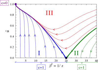
Figure 3: The flow diagram of the SG model in the scale-dependent frequency approximation. The phase space is divided into three regions. In region $I$ we have a line of UV repulsive Gaussian fixed points ($\bar{u}=0,\beta^{2}<8\pi$). Every trajectory starting in the vicinity of this line ends in an IR attractive fixed point (purple full circle, $\bar{u}=1,\beta^{2}=0$). The $\Delta c$ observed along the trajectories of this region should be equal to $1$. Region $II$ contains a line of IR attractive Gaussian fixed points ($\bar{u}=0,\beta^{2}>8\pi,$) which are the end points of trajectories starting at $\beta^{2}\approx\infty$ below the thick green line, i.e. the separatrix. Region $III$ contains those trajectories starting at $\beta^{2}\approx\infty$ which end in the IR attractive fixed point (purple full circle).

The phase diagram obtained at this approximation level is sketched in Fig.3, where we evidence three different regions. The $\Delta c$ is strictly well defined only in region $I$, where we start from a Gaussian fixed point $c_{UV}=1$ and we end up on a massive IR fixed point $c_{IR}=0$. The massive IR fixed point related to the degeneracy of the blocked action is an important feature of the exact RG flow IR1 ; IR2 ; IR3 ; IR4 and it was considered in SG type models SG_Trun ; IR_SG1 ; IR_SG2 .

In region $II$ the trajectories end in the Gaussian fixed points $c=1$ but they are coming from infinity where actually no fixed point is present. This is due to the fact that we are not considering in our ansatz (24) any operator which can generate a fixed point at $c>1$ and then the trajectories ending at $c=1$ are forced to start at infinity. Thus, $\Delta c$ is not defined in this region.

Region $III$ contains those trajectories which start at $\beta=\infty$ but end in the IR massive fixed point at $c=0$. Even in this case the $\Delta c$ is not well defined.

In the following we are going to discuss in details the results of region $I$ where all the trajectories should give $\Delta c=1$. We shall ignore region $II$ where the $\Delta c$ is not defined, briefly discussing region $III$.

The presence of wave-function renormalization is necessary to obtain the qualitative correct flow diagram for the SG. Note that Eq. (18) has been derived only in the case of scale-independent kinetic term and the derivation of an equivalent expression in the case of running wave function renormalization appears far more demanding than the calculation sketched in this paper. However, it is still possible to get a sensible result using the mapping between the running wave-function renormalization and the running frequency $\beta_{k}$ cases (as shown in Eqs. (32a) and (32b)), finally obtaining Eq. (44) In other words the equation (18) is valid only at LPA level, but it is still possible to apply it to the $z+$LPA scheme, since, thanks to the mapping described in Eqs. (32a) and (32b) the $z+$LPA ansatz can be mapped into an LPA one.

We will then use directly the ansatz,

$$\tilde{V}_{k}=\tilde{u}_{k}\cos(\beta_{k}\phi)$$ (42)

with no wave function renormalization present in the kinetic term. This ansatz is equivalent to ansatz (24) if we rescale the field and use the relations (32a) and (32b), with the running frequency playing the role of a wave-function renormalization.

Ansatz (42) is not suited to study the SG model when full periodicity has to be preserved, indeed when we substitute it into equation (27) symmetry breaking terms appear. The same happens when we substitute it into Eq.(18). However in the latter case symmetry breaking terms are not dangerous, since we have to evaluate the expression at the potential minimum where all the symmetry breaking terms vanish.

Proceeding in this way we obtain

$$k\partial_{k}c_{k}=\frac{(\beta_{k}^{2}k\partial_{k}\tilde{u}_{k}+2\tilde{u}_{k}\beta_{k}k\partial_{k}\beta_{k})^{2}}{(1+\tilde{u}_{k}\beta_{k}^{2})^{3}}$$ (43)

where no inconsistency is present.

We still cannot use expression (43), since we cannot write a flow for $\beta_{k}$ due to the non-periodic terms. To avoid these difficulties we rewrite expression (43) using the inverse transformation of (32a) and (32b),

$$k\partial_{k}c_{k}=\frac{(k\partial_{k}\tilde{u}_{k})^{2}}{(1+\tilde{u}_{k})^{3}}.$$ (44)

The last expression is fully coherent and represents the flow of the $c$-function in presence of a running wave-function renormalization into the SG model; it is worth noting that the use of transformations (32a) and (32b) gave us the possibility to derive the expression (43) from Eq (18), which was derived in c_func in the case of no-wave-function renormalization.

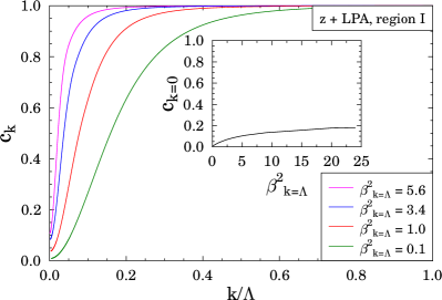
Figure 4: Running of the $c$-function obtained in the case of scale-dependent wave-function renormalization for the single-frequency SG model, as expected the case of small frequency ($\beta_{k=\Lambda}<0.1$) was already very well described by the scale-independent frequency case Fig. 1. The inset shows the results obtained for $c_{IR}$ as a function of $\beta_{k=\Lambda}$, these results show lower accuracy in the large frequency limit, while they become practically exact in the limit $\beta_{k=\Lambda}\to 0$, accordingly with c_func .

In the limit $\beta^{2}_{k=\Lambda}\to 0$, the IR result of the $c$-function (see the inset of Fig. 4) tends to zero. This implies that in the limit $\beta^{2}_{k=\Lambda}\to 0$ the difference $\Delta c\to 1$. The numerical result found in this case reaches the accuracy $1\geq\Delta c\geq 0.99$ of the scale-independent frequency solution (33) but now the periodicity of the SG model is fully preserved (which was not the case in c_func ). It should be also noted that the accurate results of Fig.4 could not be obtained in the mass cutoff framework (3a) with $b=1$, which does not allow the flow to converge, but our findings were obtained with the smoother $b=2$ cutoff.

Fig 4 reports the running of the $c$-function for various values of the initial condition $\beta_{\Lambda}$. The final $\Delta c$ value depends on the trajectory even if it should not be at exact level. This discrepancy shows that the flow obtained by approximated FRG procedure cannot satisfy the exact CFT requirements for the $c$-function.

The discrepancy between the exact $\Delta c=1$ value and the actual results obtained by the FRG approach can be used to quantify the error committed by the truncation ansatz in the description of the exact RG trajectories.

We observe that the results of Fig. 4 main and inset are obtained by using power-law regulator with $b=2$. The same computation appears to be considerably more difficult using general cutoff functions, including the exponential one.

Let us note that for vanishing frequency the RG flow equations become regulator-independent and that the $c$-function value tends to the exact result $\Delta c=1$. This justifies the accuracy obtained in c_func even though the mass cutoff was used and the periodicity violated.

Finally we go on showing the results in region $III$. As discussed in the description of Fig. 3, trajectories in region $III$ of the SG flow diagram should not have a well defined value for the $c$-function, due to the fact that those trajectories start at $\beta_{k=\Lambda}=\infty$ where no real fixed point is present.

However the numerical results obtained for those trajectories Fig. 5 are not so far from $\Delta c=1$, due to the fact that they get most of the contribution in the region where they approach the ”master trajectory” separatrix of region $I$ i.e. the blue thick line in Fig.3, which we know to have a value $\Delta c\approx 1$, while the portion of the trajectories close to region $II$ get almost zero contribute.

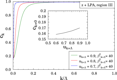
Figure 5: The flow of the $c$-function in Region $III$ of the SG flow diagram Fig. 3, the result is approximately $\Delta c=1$ due to the fact that in region $III$ most of the contribution to the $c$-function comes from the part of the trajectories very close to ”master trajectory” separatrix of region $I$ (the blue thick line in Fig. 3).

The results of region $III$ are also in agreement with the findings of region $II$ (not shown) where $\Delta c\approx 0$ for all the initial conditions.

VII Conclusions

In this paper we provided an estimation of the $c$-function over the RG trajectories of the sine-Gordon (SG) model in the whole parameter space. Using this result we showed that the numerical functional RG study of the SG model with scale-dependent frequency recovers for $\beta^{2}<8\pi$ (region I of Fig. 3) the exact result $\Delta c=1$ with a good quantitative agreement while preserving the periodicity, which is the peculiar symmetry of the model. We also pointed out the dependence of this $c$-function calculation on the approximation level considered. For $\beta=0$ one retrieves directly $\Delta c=1$, also in the scale-independent frequency case, while for $\beta\neq 0$, again using scale independent frequency, we recover this result in the $\beta^{2}\to 0$ limit, while increasing $\beta^{2}$ up to $8\pi$ in region $I$ as a result of the used approximation the agreement becomes worst, remaining anyway reasonably good, as shown in Fig. 1.

Retrieving $\Delta c=1$ is the SG counterpart of the computation of $\Delta c$ for the sinh-Gordon model fring ; dorey . This result can be understood by noticing that the analytical continuation $\beta\to i\beta$ doreybook may be expected not to alter the $\Delta c$ defined in the Zamolodchikov theorem, and that functional RG even in its crudest approximation does not spoil such correspondence for $\Delta c$, provided that the periodicity of the SG field is correctly taken into account.

We developed a fully coherent expression for the $c$-function in the case of running frequency, which gives better results in the whole region $I$ (defined in Fig. 3). These results are compatible with the exact scenario up to an accuracy of $80\%$ in the whole region $I$. Such accuracy grows to $99\%$ in the small beta region in agreement with c_func , as we discussed in Fig. 4.

We also noticed that for $\beta^{2}>0$ the use of the mass cutoff, as necessary to be consistent with expression (18), is not possible due to bad convergence properties, and the use of different $b$ values or of different cutoff types is needed.

It should be noted that while the numerical results are quite accurate the exact property that all trajectories of region $I$ should have the same value for $\Delta c$ is not preserved by truncations schemes (24) (results in Fig. 1) nor (19) (results in Fig. 4). Actually the $\beta^{2}\to 0$ limit always gives the correct result even when treated with the most rough truncation, this result being independent from the cutoff function. At variance one needs to go to the running frequency case to obtain reliable results for $\beta^{2}>>0$.

Even when full periodicity in the field is maintained, the $z+LPA$ truncation scheme is not sufficient to recover exact results for the $c$-function. Indeed the quantity computed using expression (18) satisfies two requirements of Zamalodchikov’s $c$-theorem,

1. $\partial_{t}c_{t}\geq 0$ along the flow lines,

2. $\partial_{t}c_{t}=0$ at the fixed points,

but it fails to reproduce the exact central charge of SG theory.

The final result of our calculation also depends on the chosen cutoff function and, as already mentioned, it was not possible to use the same cutoff scheme for both the couplings flow equations and the $c$-function flow (18). We do not expect these issues to be responsible for the error in the fixed point value of the $c$-function. Modifications of the cutoff scheme in LPA calculations have small influence on the results (around 5%) and we may expect this property to be maintained at $z+$LPA level, where calculations with different cutoff functions were not possible.

The main source of deviation from the exact result $\Delta c=1$ is then probably due to $z+$LPA truncation in itself. We are not able to identify whether this deviation is only due to the approximation in the $c$-function flow or rather to the description of the fixed point given in $z+$LPA, which does not reproduce the exact central charge.

Certainly the $c$-function flow at $z+$LPA level not merely violates the exact fixed point value of the $c$-function, but it is also not able to produce trajectory independent results, as shown in Fig. 4. This scenario is not consistent with an unique central charge value at the SG fixed point and it is then impossible to dig out any information about this quantity from this approach. In this perspective it would be interesting to have an independent method to calculate the fixed point central charge at a given truncation level.

Obviously the reproduction of the Zamalodchikov’s $c$-theorem should be better satisfied increasing the truncation level considered. However it has been shown that, at LPA level, the addition of further harmonics in the potential does not improve the results presented, while the introduction of running frequency is crucial to achieve consistency of the phase diagram.

This situation is peculiar of the LPA truncation level. Beyond $z+$LPA we expect the most relevant corrections from higher harmonics in the potential and only small variations are expected from the introduction of higher fields derivatives in (24)

Finally we remark that the trajectories of the other two regions do not have a definite $\Delta c$ value, however while region $II$ gives results $\Delta c\approx 0$, region $III$ has the $\Delta c$ values close to the ones obtained in region $I$ Fig. 5, due to the fact that all the trajectories in this region merge with the ”master trajectory” separatrix of region $I$ in the $k\to 0$ limit.

We conclude by observing that in our opinion a relevant future extension of this work could be the study of the $c$-function for the Ising model and for minimal conformal models in general. Our work also points out to the possible investigation with RG techniques of the analytical continuation relating the sine- and the sinh-Gordon models. From this respect we think it could be worthwhile to systematically study models interpolating between these two celebrated cases, both to highlight the roaming phenomenon for integrable interpolations and to put forward critical properties of non-integrable interpolations.

References

- (1) G. Mussardo, Statistical field theory: an introduction to exactly solved models in statistical physics (Oxford, Oxford University Press, 2010).
- (2) N. Goldenfeld, Lectures on phase transitions and the renormalization group (Reading, Addison Wesley, 1992).
- (3) J. Cardy, Scaling and renormalization in statistical physics (Cambridge, Cambridge University Press, 1996).
- (4) A. M. Polyakov, JETP Lett. 12, 381 (1970).
- (5) P. Di Francesco, P. Mathieu, and D. Sénéchal, Conformal Field Theory (New York, Springer, 1997).
- (6) A. B. Zamolodchikov, JETP Lett. 43, 730 (1986).
- (7) J. L. Cardy, Phys. Rev. Lett. 60, 2709 (1988).
- (8) A. Fring, G. Mussardo, and P. Simonetti, Nucl. Phys. B 393, 413 (1993).
- (9) P. Dorey, G. Siviour, and G. Takács, JHEP 1503, 54 (2015).
- (10) P. Minnhagen, Rev. Mod. Phys. 59, 1001 (1987).
- (11) L. P. Kadanoff, Statistical physics: statics, dynamics and renormalization (Singapore, World Scientific, 2000).
- (12) V. E. Korepin, N. M. Bogoliubov, and A. G. Izergin, Quantum Inverse Scattering Method and Correlation Functions (Cambridge, Cambridge University Press, 1997).
- (13) A. O. Gogolin, A. A. Nersesyan, and A. M. Tsvelik, Bosonization and strongly correlated systems (Cambridge, Cambridge University Press, 1998).
- (14) S. Coleman, Phys. Rev. D 11, 2088 (1975).
- (15) A. Codello, G. D’Odorico, and C. Pagani, JHEP 1407, 040 (2014).
- (16) J. Berges, N. Tetradis, and C. Wetterich, Phys. Rep. 363, 223 (2002).
- (17) J. Polonyi, Central Eur. J. Phys. 1, 1 (2004).
-
(18)
B. Delamotte, in Order, disorder and criticality:
advanced problems of phase transition theory,
Yu. Holovatch ed. (Singapore, World Scientific, 2007)
[
arXiv:cond-mat/0702365]. - (19) I. Nándori, JHEP 1304, 150 (2013).
- (20) T. R. Morris, Int. J. Mod. Phys. A 9, 2411 (1994).
- (21) D. F. Litim, Phys. Lett. B 486, 92 (2000).
- (22) I. Nándori, J. Polonyi, and K. Sailer, Phys. Rev. D 63, 045022 (2001).
- (23) I. Nándori, S. Nagy, K. Sailer, and A. Trombettoni, Phys. Rev. D 80, 025008 (2009).
- (24) I. Nándori, Phys. Rev. D 84, 065024 (2011).
- (25) S. Nagy, I. Nándori, J. Polonyi, and K. Sailer, Phys. Rev. Lett. 102, 241603 (2009).
- (26) N. Tetradis and C. Wetterich, Nucl. Phys. B 383, 197 (1992).
- (27) J. Braun, H. Gies, and D. D. Scherer, Phys. Rev. D 83, 085012 (2011).
- (28) S. Nagy, Phys. Rev. D 86, 085020 (2012).
- (29) S. Nagy, J. Krizsan, and K. Sailer, JHEP 1207, 102 (2012).
- (30) S. Nagy and K. Sailer, Int. J. Mod. Phys. A 28, 1350130 (2013).
- (31) S. Nagy, Nucl. Phys. B 864, 226 (2012); Annals Phys. 350, 310 (2014).
- (32) P. Dorey, in Conformal Field Theories and Integrable Models, Z. Horváth and L. Palla eds., Lecture Notes in Physics Volume 498, pg. 85 (Berlin, Springer-Verlag, 1997).