Election algorithms with random delays in trees

Abstract

The election is a classical problem in distributed algorithmic. It aims to design and to analyze a distributed algorithm choosing a node in a graph, here, in a tree. In this paper, a class of randomized algorithms for the election is studied. The election amounts to removing leaves one by one until the tree is reduced to a unique node which is then elected. The algorithm assigns to each leaf a probability distribution (that may depends on the information transmitted by the eliminated nodes) used by the leaf to generate its remaining random lifetime. In the general case, the probability of each node to be elected is given. For two categories of algorithms, close formulas are provided.

Key words: Distributed Algorithm, Election Algorithm, Probabilistic Analysis, Random Process.

1 Introduction

1.1 The problem

Starting from a configuration where all processors are in the same state, the goal of an election algorithm is to obtain a configuration where exactly one processor is in the state leader, the other ones being in the state lost. The (leader) election problem is often the first problem to solve in a distributed environment. A leader permits to centralize some information, to make some decisions, to coordinate the processors for subsequent tasks. Hence, the election problem – first posed by Le Lann in [6] – is one of the most studied problems in distributed algorithmic, and this under many different assumptions [9]. The graph encoding the relations between the processors can be a ring, a tree, a complete or a general connected graph. The system can be synchronous or asynchronous and processors may have access to a total or partial information of the geometry of the underlying graph, or of the current state of the system, etc.

In this paper we consider the case of election in trees, when the nodes have at time $t=0$ a very partial information on the geometry of the tree: each node only knows its number of neighbors. A possible method for electing in a tree, introduced by Angluin ([1] Theorem 4.4), amounts to eliminating successively the leaves till only one node remains, the leader. In this paper, we investigate this method in the general case: assume that a node $u$ being a leaf (was a leaf at time $t=0$, or that becomes a leaf at time $t$) decides to live a random remaining time $D_{u}$ before being eliminated; in other words, it is eliminated at time $t+D_{u}$ except if it is elected before this date. Starting with a given tree $T_{0}$ at time 0, denote by $T_{t}$ the tree constituted with the non-eliminated nodes at time $t$. The family $(T_{t})_{t\geq 0}$ is a random process taking its values in the set of trees. Given $T_{0}$, the distribution of $(T_{t})_{t\geq 0}$ – and then, also the probability that a given node is elected – depends on the way the nodes choose the distribution according to which they will compute their random remaining lifetime.
– In [7] the authors consider two elementary approaches. The first one is based on the assumption that all sequences of leaves elimination have the same probability (no distributed algorithm seems to have this property). Their second approach assumes that at each step all leaves have the same probability of being removed. This corresponds to the case where the $D_{u}^{\prime}s$ are all exponentially distributed with parameter 1. The authors study thoroughly both approaches and prove many properties of resulting random processes.
– In [8], the authors show that if the nodes suitably choose their remaining random lifetime then a totally fair election process is possible, the nodes being elected equally likely (in Section 3.2 this example is revisited). In [4] and [3], the authors extend the result from [8] to a more general class of graphs: the polyominoid graphs. They also prove a conjecture: the expected value of the election duration is equal to $\log n$.

In this paper, we investigate the general case, namely, we consider the case where a leaf $u$ generates its remaining lifetime $D_{u}$ according to a distribution ${\cal D}_{u}$, where ${\cal D}_{u}$ may depend on all the information that $u$ has at its disposal (see Remark 2 below). We warm the reader to distinguish the notation ${\cal D}_{u}$ and $D_{u}$.

Remark 1

– In order to avoid that two nodes may disappear exactly at the same time, the distributions ${\cal D}_{u}$ need to avoid atoms (points with a positive mass). Even if not recalled in the statements, we assume that the distributions ${\cal D}_{u}$ have no atom. (In Section 3.3 a case where ${\cal D}_{u}$ maybe 0 with a positive probability arises and leads to problems).

– It is assumed throughout the paper, that the nodes own independent random generators. This assumption is needed each time that the independence argument is used in the paper.

1.2 The general scheme

Throughout this paper $T=(V,E)$ is a tree in the graph theoretic sense: $V$ is its set of nodes, $E$ the set of edges. The graph $T$ is acyclic and connected, and undirected. The size of $T$, denoted by $|T|$, is the number of nodes.

In the class of algorithms we study, a node $u$ becoming a leaf at time $t$ (or which was a leaf at time $t=0$) disappears at time $t+D_{u}$ (except if it is elected before!); the quantity $D_{u}$, called the remaining lifetime of $u$, is computed locally by the leaf $u$. The description of the way $u$ chooses the distribution ${\cal D}_{u}$ is crucial: this description is in fact equivalent to the description of an algorithm using the general method of elimination of leaves. We then enter into details here.

When a leaf is eliminated, it may transmit to its unique neighbor some information (this notion will be formalized below). During the execution of the algorithm, as a result of the successive eliminations of the leaves, each internal node $u$ eventually becomes a leaf, say at time $t_{u}$. At this time, it may use the information received to compute the distribution ${\cal D}_{u}$: then, it generates a random variable $D_{u}$ following ${\cal D}_{u}$ using a random generator. After this delay (at time $t_{u}+D_{u}$), $u$ is eliminated: it may transmit some information to its (unique) neighbor, and disappears from the tree. The election goes on till eventually only one single node remains; this node is then elected.

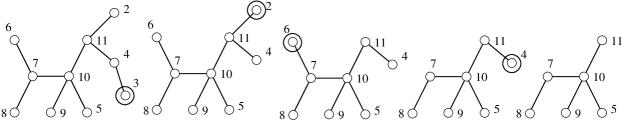
Figure 1: On this example, are circled at each step the next leaf to disappear. On this example, the remaining lifetime of the leaf 11, according to an algorithm $\Delta$ is allowed to depend on the information given by the nodes 2 and 4; the information provided by 4 may include the information it received from the node 3. The total information received by 11 has a forest structure (a forest having 2,4 as roots, and having as set of nodes $2,3,4$, and possibly containing all the lifetimes, prescribed weights, and computed values of these nodes).

As said above, the key point here is to understand that an algorithm (from the class we study) is parametrized by the way a node $u$ chooses – according to the information it has – the distribution ${\cal D}_{u}$.

We here formalize more precisely what we understand by information received and information transmitted, this needed to be coherent with the distributed model we consider. This will straightforwardly leads to the formal definition of our class of algorithms.

• The only information a node $u$ has at time 0 is its degree $\deg_{u}$ and a prescribed weight $w_{u}$, which is an element of $\mathbb{R}$, $\mathbb{R}^{d}$ or any set (this may be viewed as a personal parameter),

• at its time of disappearance a leaf $u$ transmits to its unique neighbor $v$ all the information it has:
  – the information it has received from its neighbors eliminated nodes,
  – the 4-tuple $L_{u}=(\deg_{u},D_{u},w_{u},\Gamma_{u})$ which is the local value of $u$; the quantity $\Gamma_{u}$ is computed by $u$ using the information it has received and possibly the pair $(\deg_{u},w_{u})$. In the application we have, $\Gamma_{u}$ is used to compute ${\cal D}_{u}$, and then we assume that $\Gamma_{u}$ is not a function of $D_{u}$. We call $\Gamma_{u}$ the computed value of $u$, it may belong to any set. See the remark below.

Assume that a node $u$ becomes a leaf at time $t$ when $k$ of its $k+1$ neighbors $v_{1},\dots,v_{k}$, have been eliminated. Denote by $I_{1},\dots,I_{k}$ the information these nodes have transmitted to $u$. The node $u$ has at its disposal the multiset $\{I_{1},\dots,I_{k}\}$. Recursively, one sees that the structure of the information received by $u$ is a forest with $k$ rooted trees (a forest being here a multiset of trees) rooted at the $v_{i}$’s and constituted with eliminated nodes; this forest has the geometry of the tree $T$ fringed at the $v_{i}$’s. The node $u$ formally knows the local value of each of the nodes of this forest.

Remark 2

$\bullet$ $w_{u}$ and $\Gamma_{u}$ are not used by each algorithm: when not used, they may be supposed to be 0.

$\bullet$ The notion of computed values aims to simplify the description of some algorithms, summing the needed information. Formally the transmission of this value is not necessary since it can be computed by a node having in hand all the other information.

$\bullet$ Let $\mu$ be a distribution on $\mathbb{R}$ with cumulative distribution function $F$. If $U$ is uniform on $[0,1]$ then the law of $F^{-1}(U)$ is $\mu$, where $F^{-1}(u)=\inf\{x\mid F(x)\geq u\}$ is the right continuous inverse of $F$; hence to simulate any distribution $\mu$, a uniform random variable on $[0,1]$ is sufficient. We assume that the nodes have at their disposal some independent random generators providing uniform random values on $[0,1]$.

Hence clearly, the information a node has received can be encoded without loss of information by a labelled forest $f$, where each node $v$ is labelled by the 4-tuple $L_{v}$. The set of received information will then be identified with ${\cal F}$ the set of forests labelled by 4-tuple corresponding to the $L_{u}$’s.

The other information at the disposal of a given node $u$ that may be used to compute ${\cal D}_{u}$ is its own local information $L^{\star}_{u}=(\deg(u),w_{u},\Gamma_{u})$, where as said above $\Gamma_{u}$ has been computed using $(\deg(u),w_{u})$ and the received information. We denote by ${\cal L}^{\star}$ the set of local information.

An algorithm is then just parametrized by a function $\Delta$

$$\begin{array}[]{rccl}\Delta:&{\cal F}\times{\cal L}^{\star}&\longrightarrow&\cal M\\ &(f,l^{\star})&\longmapsto&\Delta(f,l^{\star})\end{array}$$

where ${\cal M}$ is the set of probability measures having their support included in $[0,+\infty)$. The function $\Delta$ associates with a pair $(f,l^{\star})$ a probability distribution $\Delta(f,l^{\star})$. Any map $\Delta$ encodes an algorithm $\textrm{ALGO}(\Delta)$: when $\textrm{ALGO}(\Delta)$ is used, a node $u$ becoming a leaf and having received the information $f$ and having as local information $l_{u}^{\star}$, computes ${\cal D}_{u}=\Delta(f,l^{\star})$ and generates $D_{u}$ according to ${\cal D}_{u}$. The maps $\Delta$ exemplified below depend only on a part of the information received. The algorithms $\textrm{ALGO}(\Delta)$ are in the class of algorithms using the method of Angluin, and satisfy the constraints to be distributed.

Example 1

We translate into the form $\textrm{ALGO}(\Delta)$ the algorithm defined in Métivier & al. [8]. For each node $u$, $w_{u}=1$. A node which is a leaf at time 0 computes $\Gamma_{u}=1$. Let $u$ be an internal node and $\Gamma_{v_{1}},\dots,\Gamma_{v_{k}}$ be the computed values of the eliminated neighbors of $u$. Then $u$ computes:

$$\Gamma_{u}=1+\Gamma_{v_{1}}+\dots+\Gamma_{v_{k}}.$$ (1)

Now the application $\Delta$ depends only on the computed values: suppose that $u$ has received $(f,l^{\star})$ and has computed $\Gamma_{u}$, then ${\cal D}_{u}=\Delta(f,l^{\star})$ is simply ${\bf Expo}(\Gamma_{u})$, the exponential distribution with parameter $\Gamma_{u}$. Hence, ${\cal D}_{u}={\bf Expo}(1)$ if $u$ is a leaf at time $0$, and if $u$ becomes a leaf later, then ${\cal D}_{u}={\bf Expo}(\Gamma_{u})$, where $\Gamma_{u}$ equals one plus the size of the forest of eliminated nodes leading to it (see Fig. 1). It turns out that in this case, each node is elected equally likely (for all tree $T$). We provide in Section 3.2 a new proof of this fact. Métivier et al. [8], [4] and [5] introduced election algorithms on trees, $k$-trees and polyominoids having also this property.

We address the question to compute according a general $\textrm{ALGO}(\Delta)$, the probability $q_{u}$ that a given node $u$ is eventually elected. In Section 2 we answer in the general case to this question, and express the result in terms of properties of some variables arising in a related problem of directed elimination.

In the sequel, we introduce and study two categories of algorithms in the class of algorithms $\textrm{ALGO}(\Delta)$. Before discussing their properties, we have to say that in order to get close formulas for $(q_{u})_{u\in V}$, some stabilities in the computations are necessary, and this is not possible for general functions $\Delta$. The two categories we propose raise on two different kinds of stability: the $(\max,+)$ algebra in distribution, and the stable distributions for the convolutions.

– The first one is built using the properties of the exponential distribution, and generalizes the computation of Métivier & al: the application $\Delta$ takes its values in the set of exponential distributions union the set of convolutions of such distributions. This category contains an algorithm $\textrm{ALGO}(\Delta)$ such that $(q_{u})_{u\in V}$ is proportional to the prescribed weights $(w_{u})_{u\in V}$. For technical reasons the prescribed weights $(w_{u})_{u\in V}$ are to be integer valued. When the $(w_{u})_{u\in V}$ are allowed to be real numbers, we propose an algorithm which elects proportionally to these weights in case of success, but which fails with a low probability,

– the second category may be less interesting from an algorithmic point of view, since the algorithms are more time consuming than the algorithms of the first category; it has however two main advantages: it clarify in some sense the properties needed to make the computation for a given function $\Delta$, and it leads to a surprising proof of some mathematical identities involving the function $\arctan$.

2 General case: probability of a given node to be elected

In this section, we give a general formula giving $(q_{u})_{u\in V}$ for $\textrm{ALGO}(\Delta)$. The proposition below is a generalization of a proposition of Métivier &. al [8] (the coupling argument we use is new).

The idea of the proof is to decompose the event $\{u\textrm{ is not elected }\}$ into disjoint events: if $u$ is not elected, this means that $u$ has become a leaf (or was a leaf at $t=0$) and then has been eliminated. Let $t$ be the time when $u$ has become a leaf. At this time $u$ had only one neighbor $v$, and since afterward $u$ was not elected, this means that $u$ has disappeared before $v$. If at time 0, $u$ has $k$ neighbors $v_{1},\dots,v_{k}$ in the tree $T$, all of these nodes are possibly the last surviving node $v$ evoked above: the family of events

$$E_{i}=\{u\textrm{ is not elected and the last neighbor of $u$ was }v_{i}\}.$$ (2)

are the “disjoint events” mentioned above. We just have to compute $\mathbb{P}(E_{i})$.

Our idea to compute the probability of this event is to change of point of view, and to introduce a notion of directed elimination: if $u$ is eliminated before $v$, this means that the sub-tree $T[u,\cancel{v}]$ – which is defined to be the tree rooted in $u$ maximal for the inclusion in $T$ which does not contain $v$ (see Fig. 2)) – disappears entirely before $T[v,\cancel{u}]$; in the tree $T[u,\cancel{v}]$ the elimination is done from the leaves to the root $u$.

2.1 Directed elimination in rooted trees

\psfrag{u}{$u$}\psfrag{v}{$v$}\includegraphics[height=51.21504pt]{arbre.eps}

Figure 2: A tree $T$, and the two rooted trees $T[v,\cancel{u}]$ and $T[u,\cancel{v}]$

We define an algorithm $\textrm{ALGO}^{\star}(\Delta)$ (very similar to $\textrm{ALGO}(\Delta)$) which aims to eliminate all the nodes of a rooted tree, from the leaves to the root. We do not investigate the election since the last living node will be the root, but we are interested in the duration of the directed elimination of the whole tree.

We define $\textrm{ALGO}^{\star}(\Delta)$ recursively on a rooted tree $\tau$. The only difference between $\textrm{ALGO}(\Delta)$ and $\textrm{ALGO}^{\star}(\Delta)$ is that with $\textrm{ALGO}^{\star}(\Delta)$ the root of $\tau$ is never considered as a leaf: using $\textrm{ALGO}^{\star}(\Delta)$
– the leaves of $\tau$ are eliminated as with $\textrm{ALGO}(\Delta)$, transmit and receive the same information, and compute their remaining lifetimes distribution with the same function $\Delta$, but the root of $\tau$ is not considered as a leaf, even if it has only one child,
– when the root $v$ of $\tau$ becomes alone, it has received some information from its neighbors (or none if it was yet alone at time 0), then it computes using $\Delta$ the distribution ${\cal D}_{v}^{\star}$, and generate $D^{\star}_{v}$ accordingly; in other words, the root once alone behaves as a leaf in $\textrm{ALGO}(\Delta)$. After the delay $D^{\star}_{v}$, $v$ disappears.

We define the duration $D^{\star}(\tau)$ of the whole tree $\tau$ rooted in $v$ according to $\textrm{ALGO}^{\star}(\Delta)$ as the date of disappearance of $v$. If $\tau$ is a rooted tree with root $u$, and such that the subtree of $\tau$ rooted at the children of $u$ are $\tau_{1},\dots,\tau_{k}$: one has

$$D^{\star}(\tau)=D^{\star}_{u}+\max_{i}D^{\star}(\tau_{i});$$ (3)

$D^{\star}_{u}$ has a distribution given by $\Delta$ with the same rules as in $\textrm{ALGO}(\Delta)$.

We come back in the election problem in a (unrooted) tree $T$ according to $\textrm{ALGO}(\Delta)$. Let $u$ and $v$ be two neighbors in a tree $T$; consider in one hand the event

$$E_{u,v}=\{u\textrm{ is not elected and the last neighbor of $u$ is }v\}$$

corresponding to a generic event $E_{i}$ in (2). In the other hand, the two trees $T[u,\cancel{v}]$ and $T[v,\cancel{u}]$ are rooted trees, respectively in $u$ and $v$; consider two independent directed eliminations on these trees as explained above, and denote by $D^{\star}(T[u,\cancel{v}])$ and $D^{\star}(T[v,\cancel{u}])$ their independent durations. It turns out that

Proposition 1

The following identity holds true:

$$\mathbb{P}(E_{u,v})=\mathbb{P}\big{(}D^{\star}(T[u,\cancel{v}])<D^{\star}(T[v,\cancel{u}])\big{)}.$$ (4)

Proof 2.1.

We propose a proof via a coupling argument. The idea is to compare the election process which takes place in $T$ with the directed eliminations in $T[v,\cancel{u}]$ and $T[u,\cancel{v}]$, that are directed. The comparison is not immediate since these algorithms are not defined on the same probability space.

The algorithms $\textrm{ALGO}(\Delta)$ and $\textrm{ALGO}^{\star}(\Delta)$ allow each node $u$ to choose a distribution ${\cal D}_{u}$ or ${\cal D}^{\star}_{u}$ depending on the information received, from which the nodes generate their lifetimes $D_{u}$ or $D^{\star}_{u}$. According to Remark 2, a variable $U$ uniform is sufficient to generate $D_{u}$ or $D^{\star}_{u}$. Hence, we suppose that at time 0 each node $w$ in the tree $T$ has at its disposal a real number $U_{w}$ obtained by a uniform random generator on $[0,1]$. This is the key-point: a node $w$ in $T$ maybe considered also as a node in $T[v,\cancel{u}]$ or in $T[u,\cancel{v}]$, depending on which of these trees it belongs. If one now executes $\textrm{ALGO}(\Delta)$ on $T$ and $\textrm{ALGO}^{\star}(\Delta)$ on $T[u,\cancel{v}]$ and $T[v,\cancel{u}]$ using the variable $U_{w}$ for the generation of the $D_{w}$’s and the $D^{\star}_{w}$’s, one can compare the events $\{E_{u,v}\}$ and $\{D^{\star}(T[u,\cancel{v}])<D^{\star}(T[v,\cancel{u}])\}$, since they are now on the same probability space.

It turns out that for each assignment of the $U_{w}$’s, we have $\{E_{u,v}\}=\{D^{\star}(T[u,\cancel{v}])<D^{\star}(T[v,\cancel{u}])\}$. Indeed, since both algorithms use the $U_{w}$’s, since the algorithms have the same constructions and the same rules concerning $\Delta$, we see that the disappearance of leaves coincide in the two models till the disappearance of $u$ or of $v$: after this time, the information transmitted are different, and then the two processes evolve in a non comparable manner. Now, in the election process $\textrm{ALGO}(\Delta)$ in $T$, if $u$ is eliminated before $v$, then the tree $T[u,\cancel{v}]$ has lived a directed election, and thus $D^{\star}(T[u,\cancel{v}])$ coincides with the disappearance time of $u$ (for $\textrm{ALGO}(\Delta)$). At this time, since $v$ is still alive, this means that the directed elimination in $T[v,\cancel{u}]$ is not finished, thus $D^{\star}(T[u,\cancel{v}])<D^{\star}(T[v,\cancel{u}])$. Conversely, if $D^{\star}(T[u,\cancel{v}])<D^{\star}(T[v,\cancel{u}])$, then $u$ disappears before $v$ according to $\textrm{ALGO}(\Delta)$, since till the time $\min(D^{\star}(T[u,\cancel{v}]),D^{\star}(T[v,\cancel{u}]))$ the two elimination processes coincide.

We then have construct a probability space (the one where are defined the $U_{w}$’s) on which the two events $\{E_{u,v}\}$ and $\{D^{\star}(T[u,\cancel{v}])<D^{\star}(T[v,\cancel{u}])\}$ coincide; thus, they have the same probability.

As a corollary we have

Corollary 2.2.

Let $u$ be a node of a tree $T$ and $u_{1}$,…, $u_{k}$ its neighbors. Using $\textrm{ALGO}(\Delta)$

$$q_{u}=1-\sum_{1\leq i\leq k}\mathbb{P}\big{(}D^{\star}(T[u,\cancel{u}_{i}])<D^{\star}(T[u_{i},\cancel{u}])\big{)}.$$ (5)

3 First category: around the $(\max,+)$ algebra

In this category, the distribution ${\cal D}_{u}$ are either the exponential distribution or a convolution of such distributions. We will see that this category contains the algorithm of Métivier &. al. allowing to elect uniformly in the tree, an algorithm electing proportionally to positive integer valued prescribed weights, some algorithms allowing to elect proportionally to some structural features of the tree.

Before doing this, we recall some classical facts. In the sequel ${\mathcal{E}}^{[a]}$ denote a r.v. having the ${\bf Expo}(a)$ distribution, and $M_{n}=\max_{1\leq i\leq n}{\mathcal{E}}_{i}^{[1]}$ is the maximum of $n$ i.i.d. r.v. ${\bf Expo}(1)$ distributed. The distribution of $M_{n}$ is denoted from now on by ${\cal M}_{n}$ (we have $\mathbb{P}(M_{n}\leq x)=(1-\exp(-x))^{n}$, for any $x\geq 0$).

Lemma 3.3.

Let ${\mathcal{E}}^{[1]},...,{\mathcal{E}}^{[n]}$ be $n$ independent exponential random variables with parameters $1,\dots,n$. The random variables ${\mathcal{E}}^{[1]}+...+{\mathcal{E}}^{[n]}$ has distribution ${\cal M}_{n}$.

Proof 3.4.

Consider $(\hat{{\mathcal{E}}_{i}},\ 1\leq i\leq n),$ the order statistics of $n$ i.i.d. ${\bf Expo}(1)$ random variables ${\mathcal{E}}^{[1]}_{1},\dots,{\mathcal{E}}^{[1]}_{n}$, that is the sequence $({\mathcal{E}}_{i}^{[1]},\ 1\leq i\leq n),$ sorted in the increasing order. The variable $M_{n}=\max{\mathcal{E}}_{i}^{[1]}$ is also the sum of the random variables $\hat{\mathcal{E}}_{i}-\hat{\mathcal{E}}_{i-1}$, for $i=1,\dots,n$ with the convention $\hat{\mathcal{E}}_{0}=0$. Using the memoryless property of the exponential distribution, one has $\hat{{\mathcal{E}}_{i}}-\hat{{\mathcal{E}}}_{i-1}\stackrel{{\scriptstyle d}}{{=}}{\mathcal{E}}^{[n+1-i]}$ for all $i\in\{1,\dots,n\}$, and the variables $(\hat{{\mathcal{E}}_{i}}-\hat{{\mathcal{E}}}_{i-1})$ are independent (for more details, see Proposition p.19 in Feller [2]).

From the lemma we easily derive:

Corollary 3.5.

$i)$ Consider $k\geq 1$ positive integers $a_{1},\dots,a_{k}$ summing to $n$. If the r.v. $M_{a_{i}}$’s are independent, and independent of ${\mathcal{E}}^{[n+1]}$ then $M_{n+1}\stackrel{{\scriptstyle d}}{{=}}{\mathcal{E}}^{[n+1]}+\max_{1\leq i\leq k}M_{a_{i}}.$
$ii)$ For any $k\geq 1$ and $n\geq 1$, set

$$Y_{n,k}\stackrel{{\scriptstyle d}}{{=}}{\mathcal{E}}^{[n+1]}+{\mathcal{E}}^{[n+2]}+...+{\mathcal{E}}^{[n+k]},$$ (6)

where the variables ${\mathcal{E}}^{[n+i]}$ are independent. We have $M_{n+k}\stackrel{{\scriptstyle d}}{{=}}M_{n}+Y_{n,k}.$

3.1 The algorithms of the first category

The first category of algorithms we design is based on Corollary 3.5. It may be more easily understood via the directed elimination $\textrm{ALGO}^{\star}(\Delta)$, where the duration of a rooted tree $\tau$ according to $\textrm{ALGO}^{\star}(\Delta)$ will have distribution ${\cal M}_{n}$, for some $n$. The application $\Delta$ will take its values in the set of distributions $\{{\cal Y}[n,k],n\geq 1,k\geq 1\}$, where ${\cal Y}[n,k]$ is the distribution of $Y_{n,k}$ (given in (6)).

The only difference between the algorithms of the first category is the computed values $\Gamma_{u}$’s : the class of algorithm considered is then simply parametrized by the possible computed values $\Gamma$ satisfying the constraint below. It is convenient to consider bi-dimensional computed values $\Gamma_{u}=(C_{u},g_{u})$ where $C_{u}$ will be use to add some quantities coming from the received information, and $g_{u}$ is used to make some local computations.

Here are in two points the description of all the algorithms of the first category:
– At time $0$, the computed value $\Gamma_{u}$ of any leaf $u$ is $\Gamma_{u}=(0,g_{u})$ where $g_{u}$ is a positive integer. Then set

$${\cal D}_{u}={\cal Y}[0,g_{u}]\stackrel{{\scriptstyle d}}{{=}}M_{C_{u}+g_{u}}.$$ (7)

– Let $u$ be an internal node in $T$ becoming a leaf; let $f$ be the received information, and in particular let $\Gamma_{1}=(C_{1},g_{1}),\dots,\Gamma_{k}=(C_{k},g_{k})$ be the computed values of its eliminated neighbors. Then the node $u$ compute an integer value $g_{u}$ according to its information ($f$ and $L^{\star}_{u}$), and let $C_{u}=\sum_{i=1}^{k}C_{i}+g_{i}.$ Then set ${\cal D}_{u}={\cal Y}\left[C_{u},g_{u}\right].$

Let us think in terms of directed elimination. Recall that the notion of computed values are defined similarly in $\textrm{ALGO}^{\star}(\Delta)$ and in $\textrm{ALGO}(\Delta)$, but in the directed case, it is convenient to make appear the tree notation in the computed values instead of the node notation.

If a rooted tree $\tau$ is reduced to a leaf $u$, set $C(\tau)=0,g(\tau)=g_{u}$. If $\tau$ has root $u$, and if the sub-trees rooted at the children of $u$ are $\tau_{1},\dots,\tau_{k}$, then set $C(\tau)=\sum_{i=1}^{k}C(\tau_{i})+g(\tau_{i}).$ The lifetime of the root of $\tau$ is then distributed as the maximum of the $D^{\star}(\tau_{i})^{\prime}s$ plus a random variable distributed as ${\cal Y}(C(\tau),g(\tau))$.

To simplify a bit the formula, for any rooted tree $\tau$, let

$$\Theta(\tau)=g(\tau)+C(\tau).$$ (8)

Proposition 3.6.

For any algorithm $\textrm{ALGO}^{\star}(\Delta)$ of the first category the duration of a rooted tree $\tau$ satisfies

$$D^{\star}(\tau)\stackrel{{\scriptstyle d}}{{=}}M_{\Theta(\tau)}.$$

Proof 3.7.

The lifetime of a tree $\tau$ reduced to a leaf is ${\cal Y}(0,g(\tau))=M_{C(\tau)+g(\tau)}=M_{\Theta(\tau)}$. Assume by induction that the proposition is true for any rooted tree having less than $n$ nodes. Consider now $\tau$ a rooted tree with $n$ nodes and the $\tau_{i}$ defined as above. By recurrence $D^{\star}(\tau_{i})\stackrel{{\scriptstyle d}}{{=}}M_{\Theta(\tau_{i})}$, and thus, by independence of the $M_{\Theta(\tau_{i})}$’s, $D^{\star}(\tau)={\cal Y}\left[\sum_{i}\Theta(\tau_{i}),g(\tau)\right]+\max_{i}M_{\Theta(\tau_{i})}$ is in distribution equal to $M_{(\sum_{i}\Theta(\tau_{i}))+g(\tau)}\stackrel{{\scriptstyle d}}{{=}}M_{\Theta(\tau)}$ by Corollary 3.5.

As a corollary we have

Theorem 3.8.

For any algorithm $\textrm{ALGO}(\Delta)$ of the first category, any tree $T$,

$$q_{u}=1-\sum_{1\leq i\leq k}\frac{\Theta(T[u_{i},\cancel{u}])}{\Theta(T[u,\cancel{u}_{i}])+\Theta(T[u_{i},\cancel{u}])}$$ (9)

Proof 3.9.

This is a consequence of Propositions 2.2 and 3.6 and of the following identity: if $M_{a}$ and $M_{b}$ are independent, then $\mathbb{P}(M_{a}<M_{b})=a/(a+b)$.

This theorem has a direct consequence quite surprising, since it deals with very general function $\Gamma$. It is obtained by summing Equality (9) over all nodes:

Corollary 3.10.

For any tree $T$, any choice of positive integer values function $\Gamma_{u}=(C_{u},g_{u})$

$$\sum_{u}\left[1-\sum_{i}\frac{\Theta(T[u_{i},\cancel{u}])}{\Theta(T[u_{i},\cancel{u}])+\Theta(T[u,\cancel{u_{i}}])}\right]=1.$$

Remark 1 ensures that almost surely the election eventually succeeds. Indeed, each leaf eventually dies out with probability one, and then the election stops after a finite time. All the disappearance dates are different, since the lifetimes distributions have no atom: at the end it eventually remains only one leaving node which is elected.

Remark 3.11.

In general the denominator in the RHS of (9) depends on the node $u$ and, thus, apart from the two first examples below where this denominator is constant, the formula (9) cannot be “simplified”.

3.2 Examples

1. The uniform electing algorithm (treated in Example 1) is a particular case of this model by letting $g_{u}=1$ and, therefore, $\Theta(t)=|t|$, the total number of nodes in $t$. Since each node is either in $T[u,\cancel{u}_{i}]$ or in $T[u_{i},\cancel{u}]$, by (9)

   $$q_{u} = 1-\sum_{1\leq i\leq k}\frac{|T[u_{i},\cancel{u}]|}{|T[u,\cancel{u}_{i}]|+|T[u_{i},\cancel{u}]|}=1-\frac{|T\setminus\{u\}|}{|T|}=\frac{1}{|T|};$$

   this is the uniform distribution on $T$, as found by Métivier & al.

2. Assume that all prescribed weights are positive integers. If $g_{u}=w_{u}$ for every nodes then $\Theta(t)=\sum_{u\in t}w_{u}$ the total weight of the rooted tree $t$. In this case $q_{u}=\frac{w_{u}}{w(T)}$ where $w(T)=\sum_{u\in T}w(u)$ is the total weight in $T$. Indeed, in the RHS of (9) the denominator is equal to $w(T)$ whatever is the value of $i$, and summing the numerators gives $w(T)-w_{u}$.

3. For $g_{u}=\deg(u)$, $q_{u}$ becomes proportional to $\deg(u)$ (take $w_{u}=\deg(u)$ in the previous point 2).

4. In the case where $g_{u}=1$ for the leaves and $g_{u}=|t|$ more generally for all the nodes, then $\Theta(t)=PLS(t)+|t|$ becomes the path length of (the rooted tree) $t$ plus its size. Then Formula (9) gives the value of $q_{u}$.

3.3 Real-valued weights

In Example 3.2.2, we gave an algorithm of the first category such that $q_{u}$ is proportional to $w_{u}$ provided that the $w_{u}^{\prime}s$ are integers. The computations relying on Corollary 3.5, the weights have to be integer valued, or say have a known common divisor. A natural question arises: is there an algorithm such that $q_{u}$ is proportional to general real-valued weights $w_{u}$’s? We were not able to answer to this question, but using a randomized version of the algorithms of the first category, we provide an algorithm that may fail with a small probability, but such that conditionally on success, the $q_{u}$’s are indeed proportional to the $w_{u}$’s.

The difference with the algorithm described above is as follows. Instead of using its weight $w_{u}$ as a parameter in a distribution ${\cal Y}(n,k)$, a node $u$ becoming a leaf, uses its weight $w_{u}$ as a parameter of a Poisson distribution: it generates $W_{u}$ a r.v. following the Poisson($w_{u}$) distribution and then uses this integer as its weight in the description of algorithms of the first category we gave. In other words, the computed value $g_{u}$ instead of being simply $w_{u}$ will take the value $k$ with probability $\exp(-w_{u})w_{u}^{k}/k!$.
Let us discuss some points linked to the failure of the algorithm.

Remark 3.12.

– If the random generated $W_{u}$ is zero for some $u$, then conditionally to $W_{u}$ the remaining lifetime is ${\bf Expo}(0)$ distributed, that is zero almost surely: $u$ is eliminated immediately.
– If all nodes generate zero, then the algorithm fails: it terminates without choosing any node. The probability of failure for the algorithm is $e^{-w(T)}$ where $w(T)=\sum_{u\in V}w_{u}$ is the total weight. It becomes insignificant whenever $w(T)$ grows. To guarantee the success with a high probability, it suffices to multiply $w$ by a great number $c$ known by all nodes.

The following lemma, which is easily proved, simplifies the proof of the main proposition of this section.

Lemma 3.13.

Let $X_{1},...,X_{n}$ be $n$ independent r.v. of Poisson distributions with parameters ${\lambda}_{1},...,{\lambda}_{n}$ respectively. For any $k>0$, the distribution of $X_{1}$ conditionally on $X_{1}+\dots+X_{n}=k$ is binomial $B(k,\lambda_{1}/(\lambda_{1}+\dots+\lambda_{n}))$.

Proposition 3.14.

Let $T$ be any tree. The probability that the algorithm chooses a node $u$ conditioned by the event that not all nodes generate 0 is proportional to $w_{u}$ : ${\mathbb{P}}\left(u\mbox{ elected }\ \Big{|}\ \sum_{v\in V}W_{v}>0\right)={w_{u}}/{w(T)}.$

Proof 3.15.

Consider some integers $(k_{v})_{v\in V}$ , with at least one $k_{v}>0$. Given the values $W_{v}=k_{v}$ according to Section 3.2, second example, we have:

$${\mathbb{P}}\left(u\mbox{ elected }|~{}W_{v}=k_{v}\mbox{ for any }v\mbox{ in }T\right) = {k_{u}}/({\sum_{v\in V}k_{v}}).$$

Therefore the probability that the algorithm chooses $u$ conditioned by $\sum_{v}W_{v}>0$, is nothing but:

$${\mathbb{P}}(u\mbox{ elected }\Big{|}\ \sum_{v}W_{v}>0) = {\mathbb{E}}\left(\frac{W_{u}}{\sum_{v}W_{v}}\ \Big{|}\ \sum_{v}W_{v}>0\right),$$

where ${\mathbb{E}}$ denotes the expected value. But then, according to the previous lemma, for a fixed $k>0$,

$${\mathbb{E}}\left(\frac{W_{u}}{\sum_{v}W_{v}}\ |\sum_{v}W_{v}=k\right)=\frac{w_{u}}{\sum_{v}w_{v}}.$$

This implies that if the sum of generated numbers is positive, whatever the values it takes, the probability of $u$ to be elected is $\frac{w_{u}}{\sum_{v}w_{v}}$. The proposition follows.

4 Second category: around the stable distributions

The second category relies on Formula (3). One sees that choosing a suitable $D^{\star}$ may let the $\max$ operator acting on the RHS disappears: the idea is to choose $D_{u}^{\star}$ under the form

$$D_{u}=X^{u}-\max_{i}D(\tau_{i})+\sum_{i}D(\tau_{i})$$ (10)

for some $X^{u}$ whose distribution depends of the information received by $u$. In this case Formula (3) concerning the directed elimination becomes simply

$$D^{\star}(\tau)=X^{u}+\sum_{i}D^{\star}(\tau_{i}).$$

And the duration of a rooted tree satisfies:

$$D^{\star}(\tau) = X^{u}+\sum_{i}D^{\star}(\tau_{i})=\sum_{v\textrm{ nodes in }\tau}X^{v}.$$ (11)

Once again, the involved variables $X^{v}$ have a distribution that may depend on the history of the elimination of the sub-tree of $\tau$ rooted in $v$. The algorithms of the second category are parametrized by all the possible distribution for $X^{u}$ (the variables $X^{u}$ appearing in (10) and (11)).

In the case where the $X^{v}$ are i.i.d, the distribution of $D^{\star}(\tau)$ is simple: it is a sum of $|\tau|$ i.i.d. random variables, and then it is indexed by the unique integer $|\tau|$. Denoting by $S_{n}$ a sum of $n$ i.i.d. copies of $X^{v}$, according to Corollary 2.2 we have for a node $u$ having $u_{1},\dots,u_{k}$ as neighbors,

$$q_{u}=1-\sum_{1\leq i\leq k}\mathbb{P}\big{(}S_{|T[u,\cancel{u}_{i}]|}<S_{|T[u_{i},\cancel{u}]|}\big{)}.$$ (12)

There is an interesting case where the computation in (12) can be made explicitly, and leads to close formulas: the case of the stable distribution with index $1/2$. The stable distributions are the families of distribution that are stable for the convolution (see Feller [2] for more information). We say that $X$ has the stable distribution with index $1/2$ if the density of $X$ is $f(t)={\bf 1}_{t\geq 0}\frac{e^{-1/(2t)}}{\sqrt{2\pi t^{3}}}.$ If $X_{1},\dots,X_{k}$ are independent copies of $X$ then $S_{k}=X_{1}+\dots+X_{k}\stackrel{{\scriptstyle d}}{{=}}k^{2}X$. Consider now $S_{m}$ and $S^{\prime}_{n}$ two independent sums of $m$ and $n$ independent copies of $X$. One has

$$\mathbb{P}(S_{m}<S^{\prime}_{n})=\mathbb{P}(m^{2}X\leq n^{2}X^{\prime})$$ (13)

for two copies $X$ and $X^{\prime}$ of $X$. Using the density of $X$ and $X^{\prime}$, one gets $\mathbb{P}(S_{m}<S^{\prime}_{n})=\frac{2}{\pi}\arctan(n/m).$ Hence

Lemma 4.16.

For any tree $T$, for any node $u$ having $u_{1},\dots,u_{k}$ as neighbors, under the algorithm presented above

$$q_{u}=1-\sum_{1\leq i\leq k}\frac{2}{\pi}\arctan\left(\frac{|T[u_{i},\cancel{u}]|}{|T[u,\cancel{u}_{i}]|}\right).$$

In particular, since $\sum q_{u}=1$ this gives for each tree a formula related to the arctan function. We review below some examples and derive formulas.

4.1 Applications: some identities involving the $\arctan$ function

Consider the star tree with $n$ nodes: it is the tree where a node $v$ has $n-1$ neighbors, say $v_{1},\dots,v_{n-1}$. By symmetry $q_{v_{i}}$ does not depend on $i$; since $v_{i}$ has for only neighbor $v$, by Lemma 4.16

$$q_{v_{1}}=1-({2}/{\pi})\arctan(n-1).$$

Using again Lemma 4.16, one has for the center of the star tree

$$q_{v}=1-\frac{2(n-1)}{\pi}\arctan\left(\frac{1}{n-1}\right).$$

Since $q_{v}+\sum_{i=1}^{n-1}q_{v_{i}}=1$ (since a node is eventually elected with probability 1), we get for any $n\geq 2$,

$$\arctan(n-1)+\arctan(1/(n-1))=\pi/2.$$ (14)

Consider now a sequence of trees $T_{n}$ such that $T_{n}$ is formed by two stars having $\alpha_{n}+1$ and $\beta_{n}+1$ nodes with center $u$ and $v$, linked by an edge between $u$ and $v$. The election probability of any leaf is $q_{v_{i}}=1-({2}/{\pi})\arctan\left(\alpha_{n}+\beta_{n+1}\right),$ when

$$q_{u} = 1-\frac{2\alpha_{n}}{\pi}\arctan\left(\frac{1}{\alpha_{n}+\beta_{n+1}}\right)-\frac{2}{\pi}\arctan\left(\frac{\beta_{n}+1}{\alpha_{n}+1}\right)$$

$$q_{v} = 1-\frac{2\beta_{n}}{\pi}\arctan\left(\frac{1}{\alpha_{n}+\beta_{n+1}}\right)-\frac{2}{\pi}\arctan\left(\frac{\alpha_{n}+1}{\beta_{n}+1}\right).$$

Using $(\alpha_{n}+\beta_{n})q_{v_{1}}+q_{u}+q_{v}=1$ and (14), we get

$$\frac{2}{\pi}\left(\arctan\left(\frac{\alpha_{n}+1}{\beta_{n}+1}\right)+\arctan\left(\frac{\beta_{n}+1}{\alpha_{n}+1}\right)\right)=1.$$

If $\alpha_{n}/\beta_{n}\to x>0$, by continuity of $\arctan$ one obtains the famous formula

$$\arctan(x)+\arctan(1/x)={\pi}/{2}.$$

Going further, let $T_{n}$ be the sequence of trees having a path of size $k$ ($k$ nodes $u_{1},\dots,u_{k}$ such that there is an edge between $u_{i}$ and $u_{i+1}$ and such that $u_{i}$ has $\alpha_{n,i}$ other neighbors that are leaves). The probability of election of any of the $\sum\alpha_{n,i}$ leaves is $q_{l}=1-\frac{2}{\pi}\arctan(\sum\alpha_{n_{i}}+k-1)$, that of $u_{i}$ is

$$1-\frac{2}{\pi}\left[\alpha_{n,i}\arctan\left(\frac{1}{\sum\alpha_{n,i}+k-1}\right)+\arctan\left(\frac{\sum_{j>i}(\alpha_{n,j}+1)}{\sum_{j\leq i}(\alpha_{n,j}+1)}\right)+\arctan\left(\frac{\sum_{j<i}(\alpha_{n,j}+1)}{\sum_{j\geq i}(\alpha_{n,j}+1)}\right)\right].$$

Finally, assuming that for any $i$, $\alpha_{n,i}\to\alpha_{i}$ for some positive real number $\alpha_{i}$, we get by continuity, and using that the sum of all events must be 1, that for any positive real number $\alpha_{1},\dots,\alpha_{k}$,

$$\sum_{i}\left[\arctan\left(\frac{\sum_{j>i}\alpha_{j}}{\sum_{j\leq i}\alpha_{j}}\right)+\arctan\left(\frac{\sum_{j<i}\alpha_{j}}{\sum_{j\geq i}\alpha_{j}}\right)\right]=\frac{\pi}{2}(k-1).$$ (15)

Each simple finite tree used as a skeleton on which are grafted some packets of leaves (with size $\alpha_{n,k}$, $k$ corresponding to a labeling of the nodes of the skeleton) will provide a formula similar to (15).

References

- [1] D. Angluin. Local and global properties in networks of processors. In Proceedings of the 12th Symposium on theory of computing, pages 82–93, 1980.
- [2] W. Feller. An introduction to probability theory and its applications. Vol. II. Second edition. John Wiley & Sons Inc., New York, 1971.
- [3] A. El Hibaoui, J.M. Robson, N. Saheb-Djahromi, and A. Zemmari. Uniform election in polyominoids and trees. soumis à Discrete Applied Mathematics.
- [4] A. El Hibaoui, N. Saheb-Djahromi, and A. Zemmari. Polyominoids and uniform election. In 17th Formal Power Series and Algebraic Combinatorics (FPSAC), 2005.
- [5] A. El Hibaoui, N. Saheb-Djahromi, and A. Zemmari. A uniform probabilistic election algorithm in k-trees. In 17th IMACS World Congress : Scientific Computation, Applied Mathematics and Simulation (IMACS), 2005.
- [6] G. Le Lann. Distributed systems - towards a formal approach. In IFIP Congress, pages 155–160, 1977.
- [7] Y. Métivier and N. Saheb. Probabilistic analysis of an election algorithm in a tree. In Sophie Tison, editor, CAAP, volume 787 of Lecture Notes in Computer Science, pages 234–245. Springer, 1994.
- [8] Y. Métivier, N. Saheb-Djahromi, and A. Zemmari. Locally guided randomized elections in trees: The totally fair case. Inf. Comput., 198(1):40–55, 2005.
- [9] G. Tel. Introduction to distributed algorithms. Cambridge University Press, 2000.