woptic: optical conductivity with Wannier functions and adaptive k-mesh refinement

Abstract

We present an algorithm for the adaptive tetrahedral integration over the Brillouin zone of crystalline materials, and apply it to compute the optical conductivity, dc conductivity, and thermopower. For these quantities, whose contributions are often localized in small portions of the Brillouin zone, adaptive integration is especially relevant. Our implementation, the woptic package, is tied into the wien2wannier framework and allows including a many-body self energy, e.g. from dynamical mean-field theory (DMFT). Wannier functions and dipole matrix elements are computed with the DFT package Wien2k and Wannier90. For illustration, we show DFT results for fcc-Al and DMFT results for the correlated metal SrVO3.

inline,color=green!30, caption=referees]Must submit the names and institutional e-mail addresses at least 3 potential referees.

1 Introduction

The theoretical description of crystalline solids is greatly simplified by their periodicity. The Bloch theorem for non-interacting electrons allows one to replace a sum over infinitely many discrete lattice vectors by an integral over a continuous k-vector restricted to the Brillouin zone (BZ). A similar simplification is possible in interacting systems where the crystal momentum $\boldsymbol{k}$ is a conserved quantity for a variety of excitations. This makes BZ-integration an indispensable part of any numerical technique for periodic solids. To evaluate the integral numerically, we must discretize the BZ in some way. The usual methods used in band-structure calculations rely on an a priori choice of the k-mesh which covers the BZ uniformly; e.g. using a straightforward summation [1, 2, 3], or the more sophisticated tetrahedron method [4]. This is a natural choice for the calculation of quantities such as the charge density, to which all k-points contribute. On the other hand, the transport or low-energy spectral properties are usually dominated by certain regions of the BZ, e.g. the vicinity of the Fermi surface. To compute such quantities, an inhomogeneous k-mesh adapted to a particular material may be a better choice.

In the present article, we describe a technique to recursively generate an inhomogeneous k-mesh for periodic solids in three dimensions. Our implementation, the woptic package, is designed to calculate the optical conductivity, dc conductivity, and thermopower of interacting electrons. However, the adaptive k-mesh management is encapsulated in a subprogram (refine_tetra) which may easily be adapted to other quantities.

Woptic operates in the context of dynamical mean-field theory (DMFT) [5, 6] for real materials. This “DFT+DMFT” approach [7, 8] uses the band structure from density-functional theory (DFT) in the local-density or generalized gradient approximations (GGA) to construct an effective multiband Hubbard model, which is analyzed using the DMFT technique. Calculation of the optical conductivity represents a post-processing step in this scheme. In the present implementation, we use inputs generated by the Wien2k [10], wien2wannier [11], and Wannier90 [12] codes and a self energy (on the real-$\omega$ axis) from any DMFT solver. So far, only local self energies $\Sigma(\omega)$ are implemented, but the approach allows including any self energy on top of Wien2k. In particular, extension to a non-local $\Sigma({\boldsymbol{k}},\omega)$ (e.g. from $GW$ [13, 14], or from extensions of DMFT [15, 16, 17]) is simple as long as $\Sigma({\boldsymbol{k}},\omega)$ may be obtained at any ${\boldsymbol{k}}$.

When vertex corrections are neglected (they are strongly suppressed in DMFT, see Sec. 2), the optical conductivity involves a BZ sum of contributions obtained from the k-resolved one-particle spectral functions and dipole matrix elements between the corresponding wave functions. We start by evaluating the optical conductivity on a uniform tetrahedral k-mesh. Next, we offer a refinement, test the sensitivity of the studied quantity and decide, for each tetrahedron, whether the refinement should be accepted. Accepting a refinement leads to the recursive generation of additional k-points in a way that ensures the numerical stability of the algorithm.

While the band structure part of the calculation uses augmented plane waves, the Hubbard model is naturally formulated in terms of localized orbitals. The transformation between the two bases is accomplished by the Wannier construction [18, 11, 19].

An overview of the work flow of the adaptive refinement program called woptic can be found in Fig. 1. The work flow can be summarized as

1. Choose an initial k-mesh and set iteration $\ell=0$ (see Sec. 3.1 for the formal definition of the mesh).

2. Compute the dipole matrix elements $v^{(\ell)}({\boldsymbol{k}})$ of Eq. (2) (see Sec. 4 for details).

3. Compute the optical conductivity $\sigma^{(\ell)}$ for a given k-mesh (see Sec. 2 for the formula used to obtain $\sigma^{(\ell)}$). Extract the information which regions of k-space have a large contribution to the integration error (see Sec. 3.2 for details on the numerical quadrature and how the error is estimated).

4. Stop if the change of the optical conductivity with respect to the previous iteration $\sigma^{(\ell-1)}$ is below a given tolerance, otherwise refine the k-mesh where necessary, thus obtaining a new k-mesh, and return to step 1 with $\ell\leftarrow\ell+1$ (see Sec. 3.1 for information on the refinement process).

A more detailed version of the work flow, with a description of available modes, can be found in Sec. 4.2.

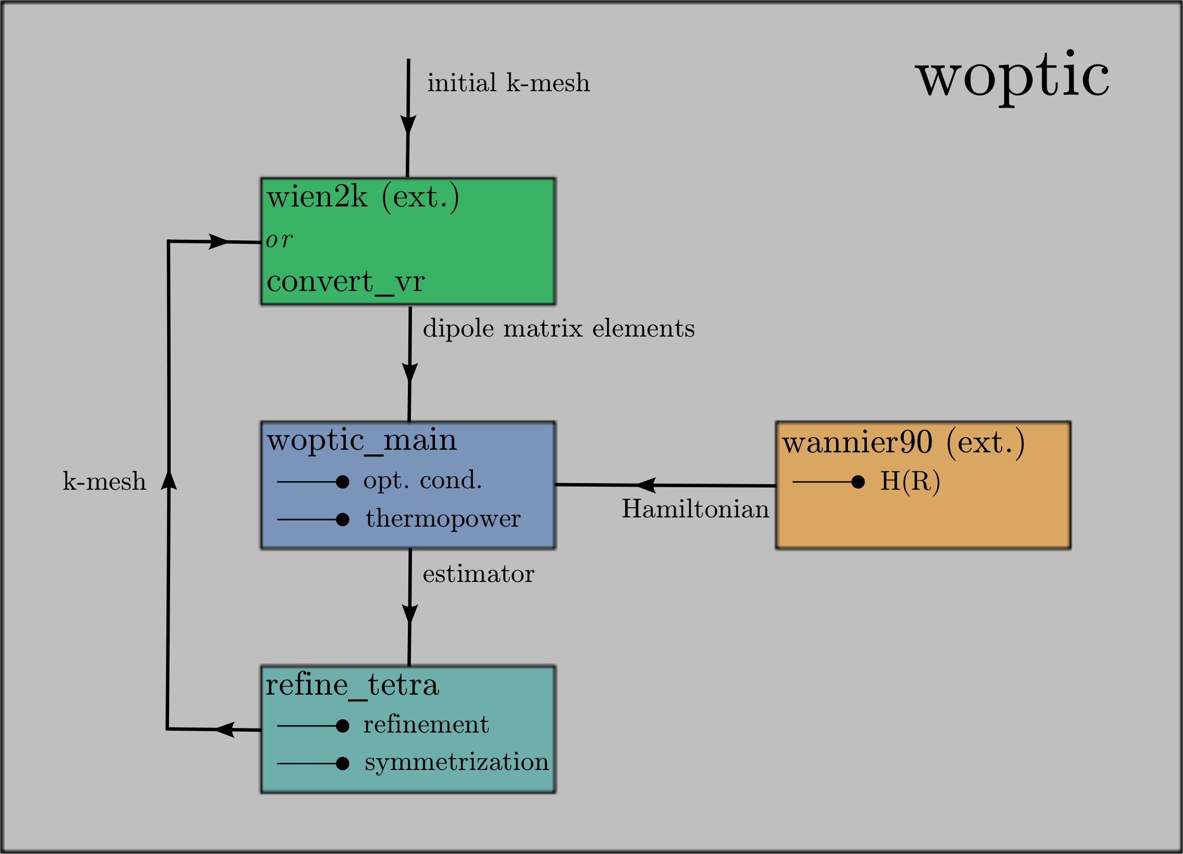
Figure 1: Schematic work flow of the woptic algorithm with an adaptive tetrahedral mesh for the Brillouin zone integration. The algorithm is implemented in two main programs woptic_main (evaluates the optical conductivity for a given k-mesh) and refine_tetra (adaptively refines the k-mesh) which are called by the driver script woptic, together with several support programs. Wannier90 provides the real space hopping matrix $H({\boldsymbol{R}})$, whereas the dipole matrix elements are computed either by the Wien2k programs lapw1 and optic, or by the woptic program convert_vr. See woptic user’s guide for more detailed work flow diagrams.

This paper is structured as follows: First, in Sec. 2, we give a description of the specific numerical problem to compute the optical conductivity. In Sec. 3, we specify the tetrahedral mesh and the refinement strategy. Furthermore, we survey the estimation of the integration error necessary to mark tetrahedra for refinement in Sec. 3.2 and depict methods to increase the numerical performance in Sec. 3.3. In Sec. 4, we focus on practical considerations such as the available modes in the program and more details of the work flow and show numerical tests. Finally, in Sec. 5 we present two applications, elementary aluminum and the vanadate SrVO3.

2 Problem statement

The Kohn-Sham Hamiltonian $H$ of DFT is diagonal in the Bloch-wave basis. Hence, the corresponding optical conductivity $\sigma$ can be written in terms of the dipole matrix elements and $\delta$-functions [20], setting $\hbar=1$,

$$\sigma_{\alpha\beta}(\Omega)=-\frac{e^{2}}{(2\pi)^{2}}\mathop{\int\limits_{\text{{BZ}}}\!d{\boldsymbol{k}}}\sum_{c,v}\frac{\delta(\varepsilon_{c}({\boldsymbol{k}})-\varepsilon_{v}({\boldsymbol{k}})-\Omega)}{\Omega}\\ \cdot v_{v,c}^{\alpha}({\boldsymbol{k}})v_{v,c}^{\beta}({\boldsymbol{k}}).$$ (1)

Here, $\Omega$ is the external frequency, $e$ is the electronic charge, the sum is over conduction ($c$) and valence ($v$) electrons with energy $\varepsilon_{c/v\,{\boldsymbol{k}}}$, while

$$v^{\alpha}_{nm}({\boldsymbol{k}})=-\frac{\text{i}}{m_{\text{e}}}\braket{\psi_{n{\boldsymbol{k}}}}{\partial_{\alpha}}{\psi_{m{\boldsymbol{k}}}}$$ (2)

are the dipole matrix elements with the Bloch states $\psi_{n{\boldsymbol{k}}}$, and $m_{\text{e}}$ denotes the electron mass. In general, the resulting value for $\sigma$ depends on the number of k-points used in the integration as well as the applied quadrature rule. However, the evaluation of the integrand in Eq. (1) is numerically cheap and one usually proceeds to uniformly refine a given k-mesh until convergence.

In the following we assume that we have constructed a mapping $U({\boldsymbol{k}})$ from $N$ Bloch states computed by Wien2k [21] to $N$ maximally localized Wannier functions (WFs) with Wannier90 [12]; thus we have the Hamiltonian in Wannier space

$$H({\boldsymbol{k}})=U^{+}({\boldsymbol{k}})E({\boldsymbol{k}})U({\boldsymbol{k}})\qquad\text{with}\qquad E_{nm}({\boldsymbol{k}})=\delta_{nm}\varepsilon_{n{\boldsymbol{k}}}.$$ (3)

This means that the electronic structure is not described in terms of bands $\varepsilon_{n{\boldsymbol{k}}}$, $1\leq n\leq N$, but by a Hamiltonian matrix $H({\boldsymbol{k}})\in{\mathbb{C}}^{N\times N}$. This is appropriate, for example, when a set of WFs is required as an input for many-body calculations such as DFT+DMFT. Also in light of possible DFT+DMFT applications of the algorithm, we will not consider the effects of vertex corrections. In fact, while they can significantly affect the DMFT results for other response functions like the spin/charge susceptibilities [22, 23], their contribution to the DMFT optical conductivity is strongly suppressed (and vanishes exactly in the single-band case) due to the k-structure of the electronic current operator [24, 25]. On the basis of these considerations, the following general expression for the optical conductivity [25, 26] can be written

$$\sigma_{\alpha\beta}(\Omega)=-\frac{e^{2}}{(2\pi)^{2}}\mathop{\int\limits_{\text{{BZ}}}\!d{\boldsymbol{k}}\!\int_{-\infty}^{+\infty}\!\!d\omega}\frac{f(\omega+\Omega)-f(\omega)}{\Omega}\cdot\\ \operatorname{Tr}\left[v^{\text{w}\alpha}({\boldsymbol{k}})A({\boldsymbol{k}},\omega+\Omega)v^{\text{w}\beta}({\boldsymbol{k}})A({\boldsymbol{k}},\omega)\right].$$ (4)

Here, $f$ is the Fermi function at a given temperature,

$$v^{\text{w}\alpha}_{rs}({\boldsymbol{k}})=U^{+}_{rn}({\boldsymbol{k}})\,v^{\alpha}_{nm}({\boldsymbol{k}})\,U_{ms}({\boldsymbol{k}})=-\frac{\text{i}}{m_{\text{e}}}\braket{w_{r{\boldsymbol{k}}}}{\partial_{\alpha}}{w_{s{\boldsymbol{k}}}}$$ (5)

the dipole matrix rotated to the basis of k-space WFs $w_{r{\boldsymbol{k}}}(\boldsymbol{r})$, and $A$ the matrix spectral function

$$A_{mn}({\boldsymbol{k}},\omega)=\frac{\text{i}}{2\pi}\left[G_{mn}^{ret}({\boldsymbol{k}},\omega)-G_{nm}^{ret,*}({\boldsymbol{k}},\omega)\right]$$ (6)

defined via the Green’s function

$$G({\boldsymbol{k}},\omega)=\big{[}\omega-H({\boldsymbol{k}})-\Sigma({\boldsymbol{k}},\omega)\big{]}^{-1}$$ (7)

and the corresponding electronic self energy $\Sigma({\boldsymbol{k}},\omega)$, all of which are also taken to be in the Wannier basis. Whereas in DFT, Eq. (1) scales linearly with the number of included bands, the general version, i.e., Eq. (4), scales quadratically with the number of orbitals. Thus, for a basis set in which $H({\boldsymbol{k}})$ is not diagonal, such as WFs, it is useful to reduce the number of k-space evaluations, while keeping the level of accuracy as close to the DFT formalism as possible.

In the specific case of DFT+DMFT calculations, the $({\boldsymbol{k}},\omega)$-resolution required to resolve all features of the integrand of Eq. (4) depends in particular on the imaginary part of the self energy $\Sigma({\boldsymbol{k}},\omega)=\Sigma(\omega)$ contained in the DMFT Green’s function $G({\boldsymbol{k}},\omega)$. For small $\Im\Sigma(\omega)$, a fine $({\boldsymbol{k}},\omega)$-mesh is needed, since

$$\operatorname{Tr}\left[v^{\text{w}}({\boldsymbol{k}})\,A({\boldsymbol{k}},\omega+\Omega)\,v^{\text{w}}({\boldsymbol{k}})\,A({\boldsymbol{k}},\omega)\right]$$ (8)

becomes sharply peaked. In many systems, the values of $\Im\Sigma(\omega)$ vary significantly between the different orbital manifolds, in particular when considering transitions between localized orbitals (which have been treated, e.g., with DMFT) and itinerant orbitals (whose description usually remains at the DFT or at the Hartree approximation level). Hence, a useful approach is to adapt the k-mesh to the problem under consideration and use a finer resolution only where it provides a substantial increase of accuracy. Though the present implementation assumes local self energies $\Sigma(\omega)$, generalization to a k-dependent $\Sigma({\boldsymbol{k}},\omega)$ is straightforward as long as $\Sigma({\boldsymbol{k}},\omega)$ can be obtained for any k-point in reciprocal space.

3 Algorithmic details

3.1 Tetrahedral mesh

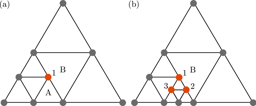
Figure 2: An example of a 2D triangulation with a hanging node (a) shown in red and marked $1$ (in this example we only discuss the nodes interior to the picture). Upon refinement of element $A$ shown in (a), one arrives at the triangulation (b) with two additional hanging nodes $2$, $3$. This triangulation violates the regularity condition, since there are two hanging nodes $1$, $2$ on the same edge. To make (b) regular we must also refine element $B$; this is the mesh closure for this triangulation.

The non-uniform triangulation of a three-dimensional domain represents a formidable numerical task. The concepts surveyed in this section are not new but combine various well-known methods, and below, we will concentrate on the definitions necessary for the rest of this paper. For a more formal and complete introduction to tetrahedral triangulation see for example Ref. [27].

We denote the set of k-points of a certain tetrahedral triangulation by $\mathcal{K}$ and the corresponding set of tetrahedra by $\mathcal{T}$. Then, $N_{\boldsymbol{k}}=|\mathcal{K}|$ is the total number of k-points, and $\mathcal{K}$ contains as elements or nodes the 3D coordinates

$$n_{m}=\left[k_{x}\quad k_{y}\quad k_{z}\right],\qquad 1\leq m\leq N_{\boldsymbol{k}}.$$ (9)

Furthermore, $\mathcal{T}$ stores a list of vertices

$$T_{m}=\left[v_{1}\quad v_{2}\quad v_{3}\quad v_{4}\right],\qquad 1\leq m\leq N_{T}$$ (10)

where $v_{1},\ldots,v_{4}\in\mathcal{K}$ and $N_{T}=|\mathcal{T}|$ is the total number of tetrahedra (in practice, we store more information for each tetrahedron than just the vertices, see Sec. 3.2). Thus, the four vertices $v_{1},\ldots,v_{4}$ are nodes that define a tetrahedron $T_{m}\in\mathcal{T}$ and are themselves elements of $\mathcal{K}$. We will use the term vertex only in connection to a specific tetrahedron, while a node is a general element of the set of k-points. A special type of node is a so-called

hanging node:

$n_{h}\in\mathcal{K}$ is a hanging node if it lies on an edge of an element $T\in\mathcal{T}$ without being a vertex of $T$.

In the 2D visualization Fig. 2(a), node 1 is not a vertex of the central triangle B and hence a hanging node. Of course, a hanging node is a vertex of other triangles (here, A).

We require $\mathcal{T}$ to fulfill the following two conditions:

regularity:

No element $T\in\mathcal{T}$ has an edge with more than one hanging node (see Fig. 2; otherwise, perform mesh closure, see below).

shape stability:

For all tetrahedra $T\in\mathcal{T}$, there is a predefined constant $c_{S}$ such that the radius of the circumscribed sphere $r_{T}$ satisfies $r_{T}^{3}/|T|\leq c_{S}$ where $|T|$ is the volume of $T$.

A large amount of the algorithmic effort in woptic is focused on keeping $\mathcal{T}$ shape stable and regular on refinement. If the ratio $r_{T}^{3}/|T|$ becomes large this indicates a highly distorted tetrahedron (also called a degenerate element) and the numerical error of the integration rules may become large. A highly non-regular mesh, on the other hand, means that nearby regions of k-space are resolved very differently, see e.g. Fig. 2(b). This often leads to unstable convergence rates since some features of the integrand may not be fully resolved.

In contrast to the 2D case of triangles, the refinement of a tetrahedron into $8$ sub-tetrahedra of equal size is not unique and, in general, the resulting elements cannot all be similar to the original tetrahedron. In the following, we will depict Ong’s idea [28] for a refinement strategy where the shape of the element is at least confined to two classes, and shape stability is thus guaranteed. This strategy is based on the triangulation of the parallelepiped defined by the three reciprocal unit vectors of the BZ into six tetrahedra of equal volume [Kuhn triangulation, Fig. 3(a)]. The resulting tetrahedra fall into two classes, in the following denoted by class $1$ and $2$. Specifically, it can be proven [28, 29] that for the refinements shown in Fig. 3, the resulting $8$ new elements of a tetrahedron will again belong to one of the two classes. Of the $8$ new elements, $4$ will share a vertex with the original tetrahedron and the other $4$ will form a central octahedron. The difference between the two refinement methods shown in Fig. 3 is how the central octahedron is split into tetrahedra. Since the triangulation of the central octahedron is not unique there are other strategies to ensure shape stability, e.g. based on the numbering of the vertices [27]. In practice, ensuring shape stability of the mesh $\mathcal{T}$ amounts to book-keeping of the classes of the tetrahedra upon refinement.

In order to satisfy the regularity of the mesh $\mathcal{T}$ upon refinement, we add an additional step after the standard refinement of elements: mesh closure [30]. This procedure refines the elements with edges where regularity is violated (see Fig. 2(b) for a 2D example of a case where mesh closure is required). This leads to neighboring tetrahedra that will only differ by one level of refinement, since any tetrahedron which is refined twice while all of its neighbors remain in the initial state will automatically produce two hanging nodes on an edge. In this case the second refinement would trigger a refinement of the neighboring tetrahedra as well. Thus, when moving through k-space, the refinement level changes “smoothly”, i.e., regions with very fine resolution will not adjoin regions with very coarse resolution. These additional refinements lead to a higher number of total tetrahedra with respect to runs without mesh closure. Experience shows however that the price paid in performance is acceptable, since mesh closure helps avoid unstable runs of the algorithm.

Summarizing, we obtain the following refinement strategy, assuming we have a regular mesh $\mathcal{T}^{(\ell)}$ from the $\ell$-th iteration of woptic (see Fig. 1) and a list of tetrahedra marked for refinement (see next section).

1. Refine all marked elements of $\mathcal{T}^{(\ell)}$ according to Fig. 3(c) and (e) for class $1$ tetrahedra, and according to Fig. 3(b) and (d) for class $2$ tetrahedra to obtain a refined mesh $\mathcal{T}^{(\ell)}_{\text{ref}}$.

2. Scan $\mathcal{T}^{(\ell)}_{\text{ref}}$ for hanging nodes.

3. Mark all elements of $\mathcal{T}^{(\ell)}_{\text{ref}}$ for refinement whose edges violate the regularity condition, i.e., have multiple hanging nodes.

4. If there are marked elements return to 1 with $\mathcal{T}^{(\ell)}_{\text{ref}}\rightarrow\mathcal{T}^{(\ell)}$, otherwise continue with $\mathcal{T}^{(\ell+1)}=\mathcal{T}^{(\ell)}_{\text{ref}}$.

This procedure gives a tree-like nested algorithm of refinement steps, which allows us to store the hanging nodes of $\mathcal{T}^{(\ell)}_{\text{ref}}$ and pass them on to the next iteration of woptic. In woptic, the refinement strategy described above is implemented by the program refine_tetra (see Fig. 1).

3.2 Integration error estimation and refinement

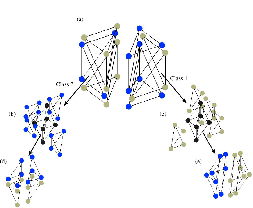
Figure 3: (a) Kuhn’s refinement of a parallelepiped into eight tetrahedra as used by the woptic program. Class $1$ tetrahedra are marked by beige vertices while class $2$ tetrahedra are marked in blue. Note that every element of class $1$ is mapped onto an element of class $2$ and vice versa if mirrored along the main diagonal plane of the cube. The tetrahedra are first refined in $4$ tetrahedra similar to the original one (having therefore the same class) and in a central octahedron denoted with black vertices, see panel (b) and (c). Depending on the class, the central octahedron is further split into $4$ tetrahedra where $2$ elements fall into the same class as the original tetrahedron and $2$ in the respective other class, see panel (d) and (e).

Having outlined the salient points of mesh management, let us now discuss how elements of a mesh $\mathcal{T}$ are chosen for refinement in the first place. Since we aim at minimizing the numerical integration error, we have to estimate the error $\epsilon_{T}$ which an element $T\in\mathcal{T}$ contributes to the overall error

$$\epsilon_{tot}=\left|\mathop{\int\limits_{\text{{BZ}}}\!d{\boldsymbol{k}}}g({\boldsymbol{k}})-\sum_{T\in\mathcal{T}}g_{T}\right|,$$ (11)

where $g({\boldsymbol{k}})$ denotes the integrand of the optical conductivity

$$\sigma_{\alpha\beta}(\Omega)=\mathop{\int\limits_{\text{{BZ}}}\!d{\boldsymbol{k}}}\left(-\frac{e^{2}}{(2\pi)^{2}}\right)\mathop{\int_{-\infty}^{+\infty}\!\!d\omega}\frac{f(\omega+\Omega)-f(\omega)}{\Omega}\cdot\\ \operatorname{Tr}\left[v^{\text{w}}({\boldsymbol{k}})A({\boldsymbol{k}},\omega+\Omega)v^{\text{w}}({\boldsymbol{k}})A({\boldsymbol{k}},\omega)\right]\\ \mathbin{=:}\mathop{\int\limits_{\text{{BZ}}}\!d{\boldsymbol{k}}}g({\boldsymbol{k}})$$ (12)

and $g_{T}$ denotes an adequate tetrahedral quadrature rule (in $g({\boldsymbol{k}})$ we omitted the dependence on the external frequency $\Omega$ for the moment, see below). For the integration over the internal frequency $\omega$, we use a straightforward summation, exploiting only the weight factor $f(\omega+\Omega)-f(\omega)$ to limit the range of integration. For the k-integration we use two different rules: First, a linear $4$-point rule

$$g_{T}^{\text{4p}}=\frac{1}{4}\sum_{i=1}^{4}g(v_{i})$$ (13)

with $v_{1},\ldots,v_{4}$ being the vertices of $T$. Second, rule (13) can also be applied to the refined elements as

$$g_{T}^{\text{4pr}}=\frac{1}{32}\sum_{j=1}^{8}\sum_{i=1}^{4}g(v_{ji}),$$ (14)

where $v_{ji}$ is the $i$-th vertex of the tetrahedron $T_{j}$ ($j=1,\ldots,8$) obtained from a refinement of $T$ as introduced in the previous section. In the implementation, we evaluate the function $g({\boldsymbol{k}})$ on the $10$ points required to apply both rules Eq. (13) and (14). The $4$ vertices of $T$ required for the rule 4p are also included in $T_{1},\ldots,T_{8}$. The latter additionally have $6$ midpoints on the edges of $T$. Thus, $T_{m}\in\mathcal{T}$ is represented by the $10$ nodes plus the class of the tetrahedron (which is required for the refinement strategy, see previous section),

$$T_{m}=\left[v_{1}\ v_{2}\ v_{3}\ v_{4};\ n_{12}\ n_{13}\ n_{23}\ n_{14}\ n_{23}\ n_{34};\ 1\text{ or }2\right],$$ (15)

where $n_{ij}$ is the midpoint between the vertices $v_{i}$ and $v_{j}$. Note that the nested nature of our quadrature rules allows us to re-use values of $g({\boldsymbol{k}})$ in following iterations of the algorithm.

To estimate the contribution which $T$ adds to the total error $\epsilon_{tot}$, we compare the results of Eqs. (13) and (14), which means that the same rule is compared for two different levels of refinement [31]. Thus, our error estimator is

$$\epsilon_{T}=\left|\int\limits_{T}\!d{\boldsymbol{k}}\ g({\boldsymbol{k}})-g^{\text{4pr}}_{T}\right|\sim\left|g_{T}^{\text{4p}}-g_{T}^{\text{4pr}}\right|.$$ (16)

Since the rule (14) is obtained by applying the rule (13) to the sub-elements $T_{1},\ldots,T_{8}$ which would be new elements if $T$ was refined, the error estimate $\epsilon_{T}$ provides a measure of how much a refinement of $T$ would improve the numerical integration.

The dependence of the optical conductivity $\sigma_{\alpha\beta}(\Omega)$ on the external frequency $\Omega$ and the directional dependence ($\alpha\beta$) have been neglected so far. To take these dependencies into account, all error estimates of an element are averaged,

$$\bar{\epsilon}_{T}=\frac{1}{6}\frac{1}{N_{\Omega}}\sum_{\Omega\alpha\beta}\epsilon^{\alpha\beta}_{T}(\Omega),\qquad\alpha\beta\in\{xx,xy,xz,yy,yz,zz\}.$$ (17)

To mark certain elements for refinement, we apply a standard procedure for adaptive mesh algorithms [30]: an element $T$ is marked if

$$\bar{\epsilon}_{T}\geq\Theta\ \max_{T^{\prime}\in\mathcal{T}}\bar{\epsilon}_{T^{\prime}},$$ (18)

where $\Theta\in[0,1]$ is a parameter determining the harshness of the refinement. A value of $\Theta=0$ means that all elements satisfy (18), i.e. uniform refinement, whereas large values of $\Theta$ lead to highly adaptive meshes. In woptic, the error estimation is partly performed by woptic_main and partly by refine_tetra (see Fig. 1). The former computes the integrand, the latter calculates the error estimators $\bar{\epsilon}_{T}$ and marks the elements for refinement according to Eq. (18).

In metallic cases, the optical conductivity $\sigma(\Omega)$ for $\Omega\rightarrow 0$ has a Drude contribution corresponding to a Lorentzian at $\Omega=0$ which is broadened by $\Im\Sigma(0)$. Thus, if $\Im\Sigma(0)$ is small, the error estimator (17) is often dominated by the values around the Fermi level $\Omega=0$ and the algorithm mainly resolves the Fermi surface. This behavior may be adequate when one is interested in the dc-conductivity or the thermopower, but for the optical inter-orbital transitions at higher energies one might favor a better description in that region. In this case, another error estimator instead of Eq. (17) is more appropriate:

$$\bar{\epsilon}^{\prime}_{T}=\frac{1}{6N_{\Omega}}\sum_{\Omega\alpha\beta}\Omega\,\epsilon^{\alpha\beta}_{T}(\Omega)\qquad\alpha\beta\in\{xx,xy,xz,yy,yz,zz\},$$ (19)

where the additional factor $\Omega$ attributes a larger weight to the error at higher frequencies.

3.3 Performance and symmetry considerations

Given that one evaluation of the function $g({\boldsymbol{k}})$ from Eq. (12) is numerically expensive, the number of total evaluations should be kept as small as possible. For this reason, we use two techniques: ($i$) re-using the data from previous iterations and ($ii$) taking into account the symmetries of the crystal. The first point is the main reason for choosing the two nested quadrature rules Eqs. (13) and (14), since, as mentioned above, a refinement of an element $T\in\mathcal{T}$ yields at most $6$ new nodes. Moreover, neighboring elements with similar refinement level share nodes with $T$. Thus, though our integration rules are of low order, they represent an efficient choice in terms of the number of total evaluation points.

To understand ($ii$), i.e. how to increase the performance by symmetry, let us define matrices $\mathcal{S}\subset{\mathbb{R}}^{3\times 3}$ describing the symmetry operations of the crystal in a Cartesian coordinate system. Furthermore, $\mathcal{K}_{s}\subseteq\mathcal{K}$ denotes the symmetrized k-mesh, i.e. the reduced mesh when the symmetry operations of $\mathcal{S}$ are exploited, with the corresponding mapping $m_{s}:n\mapsto n_{s}$ such that $n\in\mathcal{K}$ and $n_{s}\in\mathcal{K}_{s}$. If one replaces each vertex $v$ of each element of $\mathcal{T}$ by its reduced vertex $m_{s}(v)$, one formally obtains a new tetrahedral mesh $\mathcal{T}_{s}$. Note that $\mathcal{T}_{s}$ might include elements that do not correspond to real tetrahedra but have e.g. equal nodes when multiple vertices of an element of $\mathcal{T}$ have been mapped onto the same k-point in the reduced set $\mathcal{K}_{s}$. After the mapping $\mathcal{T}\rightarrow\mathcal{T}_{s}$ there are in general multiple occurrences of an element $T_{s}$. For simplicity, $\mathcal{T}_{s}$ in the following denotes the reduced symmetrized mesh, i.e. all elements $T_{s}\in\mathcal{T}_{s}$ are only considered once and carry a weight $w_{T_{s}}$, which accounts for the volume and multiplicity of $T_{s}$.

The numerical quadrature to yield the optical conductivity according to Eq. (11) is given by

$$\sigma=\sum_{T\in\mathcal{T}}g_{T}.$$ (20)

It is important to stress here that one cannot simply replace $n\in\mathcal{K}$ within the rule $g_{T}$ by $m_{s}(n)\in\mathcal{K}_{s}$, since $\sigma$ and $g_{T}$ are tensors. Hence, rotated quantities have to be used:

$$\sigma=\frac{1}{|\mathcal{S}|}\sum_{W_{s}\in\mathcal{S}}\sum_{T_{s}\in\mathcal{T}_{s}}w_{T_{s}}W_{s}^{+}g_{T_{s}}W_{s}.$$ (21)

In this approach it is sufficient to compute $g(n_{s})$ for $n_{s}\in\mathcal{K}_{s}$ and this, depending on the symmetry of the problem, may yield a considerable speed-up.

4 Practical usage

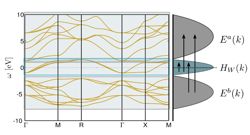
Figure 4: Possible optical transitions and corresponding Hamiltonians according to Eq. (26) for various manifolds in a low energy model for SrVO3. In the schematic visualization of the spectrum, the $\text{t}_{2g}$ manifold where the Wannier projection is performed is marked $H_{W}(k)$ and other parts of the spectrum $E^{a/b}({\boldsymbol{k}})$.

After the general description of the algorithm in the previous section, let us now turn to the connections of woptic to the program packages Wien2k and Wannier90, the available modes of operation and a more detailed work flow. As a prerequisite to start a woptic calculation, two other packages are needed: Wien2k [21] (including wien2wannier [11]) and Wannier90 [12]. This set of programs allows constructing maximally localized WFs from Wien2k (see Refs. [11, 32] for a detailed description).

To employ the adaptive integration described in the previous section, we have to be able to generate the dipole matrix $v^{\text{w}}({\boldsymbol{k}})$ and the Hamiltonian $H({\boldsymbol{k}})$ at arbitrary, a priori unknown, k-points. Two approaches are implemented in woptic: (1) matrix elements between WFs can be obtained by Fourier transformation from direct space — this is called called interp mode in the program; or (2) these matrix elements can be recomputed by Wien2k every iteration — optic mode.

Two issues are central in the following:

Gauge invariance

of the optical conductivity (4) and other observables, i.e. the independence of the random gauge of the Bloch states. While the trace in Eq. (4) is gauge invariant, its building blocks $v^{\text{w}}({\boldsymbol{k}})$ and $A({\boldsymbol{k}},\omega)$ are not. It is therefore essential that they be expressed in the same gauge.

Mixed transitions,

dipole transitions between Wannier states on the one hand, and Bloch states that are not included in the initial Wannier projection on the other.

Gauge invariance is easily ensured if approach 1 (interp mode) is available. The Wannier construction consists in finding a k-smooth gauge on the initial k-mesh $\mathcal{K}_{\text{w}}$. This amounts to finding a set of unitary matrices $U({\boldsymbol{k}})$ which represent the transformation from the initial, “random” gauge to the new gauge [19]. One then expresses the Kohn-Sham Hamiltonian and the dipole matrix elements in the new gauge using Eqs. (3) and (5), to repeat:

$$H({\boldsymbol{k}})=U^{+}({\boldsymbol{k}})\,E({\boldsymbol{k}})\,U({\boldsymbol{k}})\qquad\text{with }E_{nm}({\boldsymbol{k}})=\delta_{nm}\varepsilon_{n{\boldsymbol{k}}},$$

$$v^{\text{w}}({\boldsymbol{k}})=U^{+}({\boldsymbol{k}})\,v({\boldsymbol{k}})\,U({\boldsymbol{k}}).$$

The smoothness of the the Wannier gauge guarantees that the corresponding basis functions (i.e. the WFs) are exponentially localized, and hence that the Fourier transforms of the Hamiltonian

$$H_{rs}({\boldsymbol{R}}) =\frac{1}{N_{\boldsymbol{k}}}\sum_{{\boldsymbol{k}}\in\mathcal{K}_{\text{w}}}H({\boldsymbol{k}})\,\text{e}^{-\text{i}{\boldsymbol{k}}\cdot{\boldsymbol{R}}}=\braket{w_{r{\boldsymbol{0}}}}{\hat{H}}{w_{s{\boldsymbol{R}}}}$$ (22)

and dipole matrix elements

$$v_{rs}^{\text{w}}({\boldsymbol{R}}) =\frac{1}{N_{\boldsymbol{k}}}\sum_{{\boldsymbol{k}}\in\mathcal{K}_{\text{w}}}v^{\text{w}}({\boldsymbol{k}})\,\text{e}^{-\text{i}{\boldsymbol{k}}\cdot{\boldsymbol{R}}}=-\frac{\text{i}}{m_{\text{e}}}\braket{w_{r{\boldsymbol{0}}}}{\partial_{\alpha}}{w_{s{\boldsymbol{R}}}}$$ (23)

converge rapidly with the mesh spacing of $\mathcal{K}_{\text{w}}$. (Here and below, $w_{r{\boldsymbol{R}}}(\boldsymbol{r})$ is a direct-space WF.)

Thus we obtain direct space hopping and dipole parameters for all the significant neighbor shells (exponentially small contributions of the tails of the WFs are neglected). Having the direct space representation allows us to compute the matrix elements at an arbitrary k-point $\boldsymbol{q}$ outside $\mathcal{K}_{\text{w}}$ via

$$H(\boldsymbol{q})= \sum_{{\boldsymbol{R}}\in\mathcal{R}_{\text{w}}}H({\boldsymbol{R}})\,\text{e}^{\text{i}\boldsymbol{q}\cdot{\boldsymbol{R}}},$$ (24)

$$v^{\text{w}}(\boldsymbol{q})= \sum_{{\boldsymbol{R}}\in\mathcal{R}_{\text{w}}}v^{\text{w}}({\boldsymbol{R}})\,\text{e}^{\text{i}\boldsymbol{q}\cdot{\boldsymbol{R}}}.$$ (25)

To emphasize, the ${\boldsymbol{R}}$-sums run over $\mathcal{R}_{\text{w}}$, the set of lattice vectors dual to $\mathcal{K}_{\text{w}}$, but the localization of the WFs allows us to apply the reverse Fourier transform for $\boldsymbol{q}\notin\mathcal{K}_{\text{w}}$ with excellent accuracy. This procedure is known as Wannier interpolation [33, 34].

Mixed transitions arise when we want to extend the optical conductivity, which we have written in Eq. (4) in terms of a trace over the WFs (inner or Wannier window), to include states not covered by the Wannier projection (outer or Bloch window). The motivation for the outer window is normally to compute the optical conductivity over a larger frequency range (see Fig. 4 for a visualization of the model and the possible transitions).

For a DFT+DMFT calculation, the self energy $\Sigma(\omega)$, describing correlation effects beyond GGA, has to be provided on the real axis. In the following, this situation is referred to as interacting. Woptic also provides the option to set the self energy to a small imaginary constant $\Sigma(\omega)\equiv-\text{i}\delta$ to mimic broadening, e.g. from impurity scattering. We will refer to bands treated in this way as non-interacting. By supposition, the Bloch states in the outer window are adequately described in DFT and thus non-interacting in this sense.

When an outer window is included, we split the Hamiltonian, Wannier transformation, and dipole matrices into Wannier, Bloch, and mixed parts. Likewise, the trace in the optical conductivity (4) splits into Wannier–Wannier, Wannier–Bloch, and Bloch–Bloch terms. Denoting the diagonal energy matrix connected to the states above (below) the WFs in energy by $E^{a\,(b)}({\boldsymbol{k}})$, we can write the “large” Hamiltonian, which is block-diagonal,

$$\mathcal{H}({\boldsymbol{k}}) =\begin{pmatrix}E^{b}({\boldsymbol{k}})&&\\ &H({\boldsymbol{k}})&\\ &&E^{a}({\boldsymbol{k}})\\ \end{pmatrix}.$$ (26)

Analogously, the large Wannier transformation matrix is

$$\mathcal{U}({\boldsymbol{k}}) =\begin{pmatrix}\mathbbm{1}&&\\ &U({\boldsymbol{k}})&\\ &&\mathbbm{1}\\ \end{pmatrix}.$$ (27)

It affects only the inner window and leaves the outer window unchanged. Additionally, we have the large dipole matrix $$\mathcal{V}^{\alpha}_{mn}({\boldsymbol{k}})=-\frac{\text{i}}{m_{\text{e}}}\braket{\psi_{m{\boldsymbol{k}}}}{\partial_{\alpha}}{\psi_{n{\boldsymbol{k}}}} n,m \mathcal{H}({\boldsymbol{k}}) \mathcal{A}({\boldsymbol{k}},\omega)$$ with the indices running now over all bands in the outer window instead of only the inner window. Inserting into Eqs. (7) and (6) yields the block-diagonal matrix spectral function of the large system. Together with the large dipole matrix in the Wannier basis

$$\mathcal{V}^{\text{w}}({\boldsymbol{k}}) =\mathcal{U}^{+}({\boldsymbol{k}})\,\mathcal{V}({\boldsymbol{k}})\,\mathcal{U}({\boldsymbol{k}})$$

$$=\begin{pmatrix}(v_{ij}^{\alpha})&(v_{rj}^{\text{u}})&(v_{kj}^{\alpha})\\[3.0pt] (v_{is}^{\text{u}})&(v_{rs}^{\text{w}})&(v_{ks}^{\text{u}})\\[3.0pt] (v_{il}^{\alpha})&(v_{rl}^{\text{u}})&(v_{kl}^{\alpha})\\[3.0pt] \end{pmatrix},$$ (28)

this spectral function can be used in Eq. (4) to give a more complete description of optical transitions in the system.

Approach 1 (interp) is straightforward for the Wannier–Wannier transitions, but not directly applicable to the mixed dipole matrix elements

$$v^{\text{u}}_{ri}({\boldsymbol{k}})=\sum_{n}U^{+}_{rn}({\boldsymbol{k}})\,v^{\alpha}_{ni}({\boldsymbol{k}})=-\frac{\text{i}}{m_{\text{e}}}\braket{w_{r{\boldsymbol{k}}}}{\partial_{\alpha}}{\psi_{i{\boldsymbol{k}}}}$$ (29)

because their Fourier transform $v^{\text{u}}_{ri}({\boldsymbol{R}})$ does not decay with $|{\boldsymbol{R}}|$. To salvage Wannier interpolation in the presence of an outer window, we define the quantity

$$w^{\alpha\beta}_{rs}({\boldsymbol{k}},\omega)=\sum_{i}v^{\text{u}\alpha}_{ri}A^{a,b}_{ii}({\boldsymbol{k}},\omega)v^{\text{u}\beta}_{is}$$ (30)

where the index $i$ runs over all non-Wannier states (which are non-interacting, hence their matrix spectral function $A^{a,b}$ is diagonal). Its Fourier transform $w^{\alpha\beta}({\boldsymbol{R}},\omega)$ decays with $|{\boldsymbol{R}}|$, albeit more slowly than $v^{\text{w}}({\boldsymbol{R}})$ [35].

With these two interpolated quantities, and using the Wien2k programs lapw1 and optic [20] to compute the Bloch energies $E^{a,b}(\boldsymbol{q})$ and Bloch–Bloch dipole matrix elements $v^{\alpha}_{ij}(\boldsymbol{q})$, we can evaluate the trace (8) at any new k-point. On the other hand, the interpolation errors from $w^{\alpha\beta}(\boldsymbol{q},\omega)$ may get large, see next section and Ref. [35] for tests. (Interpolation errors from $v^{\text{w}}(\boldsymbol{q})$ are insignificant so long as properly localized WFs are found.)

As an alternative in the mixed case, we turn to approach 2 (optic mode): computing $\mathcal{V}(\boldsymbol{q})$ and $E^{a,b}(\boldsymbol{q})$ at new k-points using lapw1 and optic. (The Hamiltonian $H(\boldsymbol{q})$ is still computed using Eq. (24).) Because the (inner-window) spectral function $A(\boldsymbol{q},\omega)$ is computed in the Wannier basis, but optic yields the dipole matrix elements in the Bloch basis, we need the Wannier transformation $U(\boldsymbol{q})$ on the new k-points to mediate between them. Since the Bloch basis is the one in which the Hamiltonian is diagonal, we can obtain $U(\boldsymbol{q})$ by diagonalizing $H({\boldsymbol{k}})$ (inverting Eq. (3)).

The problem with approach 2 (optic) lies in the arbitrariness of the Bloch gauge. Since the $U(\boldsymbol{q})$ obtained via Wannier interpolation are computed by diagonalization, they are determined only up to the phases of the respective eigenvectors. In the non-interacting case, where the matrix spectral functions are diagonal, these phases evidently cancel in the trace (8); in fact, this reasoning can be extended to the interacting case as long as the Wannier self energy is a scalar (diagonal in and independent of the orbital index), e.g., because of crystal symmetry.

From a different point of view, the Bloch states $\psi_{n{\boldsymbol{k}}}$, obtained as solutions of independent eigenproblems at each k-point, carry “random” phases. The original $U({\boldsymbol{k}})$ from Wannier90 take these phases into account in constructing smooth functions $w_{r{\boldsymbol{k}}}(\boldsymbol{r})=\sum_{n}U_{nr}({\boldsymbol{k}})\,\psi_{n{\boldsymbol{k}}}(\boldsymbol{r})$ of ${\boldsymbol{k}}$. These phases are included both in $U({\boldsymbol{k}})$ and $v^{\alpha}({\boldsymbol{k}})$ and hence cancel when calculating the dipole matrix elements in Wannier space using Eq. (28).

However, if the adaptive k-mesh algorithm now selects a new point $\boldsymbol{q}$, the phase of $\psi_{n\boldsymbol{q}}$ is included in the recalculated $v^{\alpha}(\boldsymbol{q})$ but not in $U(\boldsymbol{q})$ obtained as explained above. Hence, the “random” phase may enter into the trace (8) both through the Wannier–Wannier and the mixed transitions (for the Bloch–Bloch transitions it cancels). The resulting random-gauge problem leads to errors in the results whose magnitude is a priori unknown.

So far we have assumed that the transformation between the Bloch and Wannier states at each k-point is accomplished by a unitary matrix $U({\boldsymbol{k}})$. This excludes the disentanglement procedure [36] implemented in Wannier90, where additionally a rectangular matrix $V({\boldsymbol{k}})$ intervenes. In fact, woptic supports disentanglement only in interp mode without an outer window (Wannier–Wannier transitions only). It is not clear how the method may be extended to the general disentangled case [35].

4.1 Benchmarks of interpolation and random-gauge errors

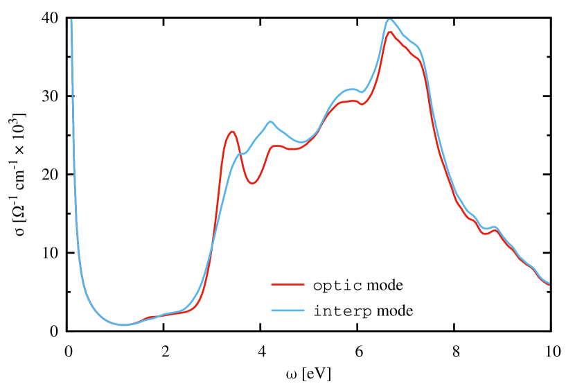
Figure 5: Optical conductivity of SrVO3 computed in the optic (red curve) and interp (blue curve) modes. For this model, whose self energy is orbital-independent due to the cubic symmetry, optic mode can be considered exact. Thus the difference between the curves reflects the interpolation errors afflicting the mixed (Wannier–Bloch) transitions in interp mode. Note that the outer window of included bands is smaller here than in Fig. 9, which is why the optical conductivity starts to drop off above $\omega\approx$7\text{\,}\mathrm{eV}$$. Here, the Wannier projection comprises the 3 V-$\text{t}_{2g}$ bands and 14 bands are included in the outer window, corresponding to O-p and V-d states.

In Fig. 5, we compare the optical conductivity of SrVO3 from the optic and interp modes, including a self energy from DMFT on the V-$\text{t}_{2g}$ states (see Sec. 5.2 for details on the DMFT calculation). Since in this material the self energy is orbital independent by symmetry, there is no random-gauge problem, and this case can be regarded as a test for the Wannier interpolation of $v^{\text{w}}$ and $w^{\alpha\beta}$.

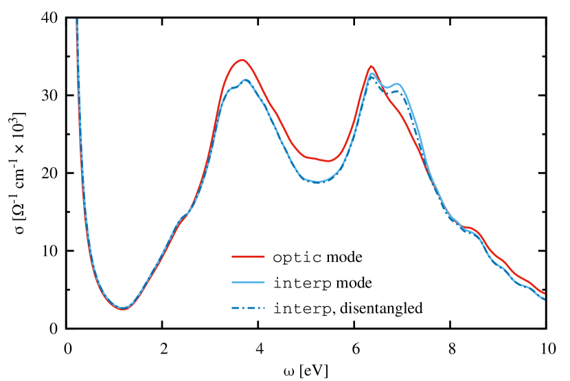
Figure 6: Optical conductivity of a model derived from SrVO3 by imposing the self energy from the 3-band model on the $\text{t}_{2g}$-like orbitals in a 14-band Wannier projection, which includes the same bands as in Fig. 5: O-p, V-$\text{t}_{2g}$, and V-$\text{e}_{g}$. For this model without mixed transitions, interp mode can be considered exact, thus the difference reflects the random-gauge errors in optic mode. The dashed blue curve is from interp mode using a Wannier projection with disentanglement of the Sr-s bands crossing the V-$\text{e}_{g}$ bands at the $R$ point of the Brillouin zone [35]. Since this corresponds to a somewhat different model, complete agreement with the solid blue curve cannot be expected.

In order to quantify the random-gauge errors, we require a test case which is complementary to the one of Fig. 5, i.e., where interpolation is reliable, but the gauge problem is in effect. To this end, we construct a Wannier projection covering exactly those bands of SrVO3 included in Fig. 5, and apply the V-$\text{t}_{2g}$ self-energy from Fig. 5 to the $\text{t}_{2g}$-derived orbitals of this larger projection. Since all included transitions are now between WFs, we need to interpolate only $v^{\text{w}}$, and can rely on interp mode as a reference; but since we apply a non-trivial self energy only to the $\text{t}_{2g}$ orbitals, $\Sigma_{i}(\omega)$ is now strongly orbital-dependent and optic mode suffers from the gauge problem. The results are shown in Fig. 6.

Comparing Figs. 5 and 6, we find that the errors from $w^{\alpha\beta}$ interpolation and from the random-gauge problem are similar in magnitude. In both cases, the qualitative features are preserved. The quantitative differences must be viewed in relation to other sources of uncertainty in these calculations. Most importantly, in DMFT the self energy on the real-$\omega$ axis is typically obtained through analytic continuation from the imaginary-$\omega$ axis. This leads to uncertainties which can easily be comparable to the errors observed in Figs. 5 and 6. It also bears mentioning that the orbital symmetry which protects optic mode from the random-gauge problem is broken especially sharply in the 14-band model used above (nontrivial $\Sigma(\omega)$ on the $\text{t}_{2g}$ orbitals, $\Sigma_{i}=-\text{i}\delta$ on the others).

Fig. 6 contains a third curve, which corresponds to interp mode on a model constructed with disentanglement. At the $R$ point of the BZ, the V-$\text{e}_{g}$ bands are entangled with Sr-s bands, as seen in the band structure of Fig. 4. These unwanted bands can be removed using disentanglement [36]. The corresponding curve in Fig. 6 is practically identical to the one without disentanglement, except for the region around $7\text{\,}\mathrm{eV}$, where transitions involving the entangled states are relevant.

For details on the issues discussed in the preceding paragraphs (to wit: the random-gauge problem in optic mode, interpolation of $v^{\text{w}}$ and $w^{\alpha\beta}$, and disentanglement in relation to woptic), we refer to Ref. [35].

4.2 Program details

To summarize, woptic offers two main choices for the matrix element mode (corresponding to the program parameter matelmode). This choice determines the method to compute the dipole matrix elements $v({\boldsymbol{k}})$. The modes and corresponding keywords in the woptic input file are:

Wannier interpolated dipole matrix elements (interp):

Apply Wannier interpolation (25) to the dipole matrix elements $v^{\text{w}\alpha}_{rs}({\boldsymbol{k}})$ in the Wannier gauge (5), as well as to the Hamiltonian (3). In the presence of an outer window, the mixed transitions are calculated from the quantity $w_{rs}({\boldsymbol{k}},\omega)$ (30), which is likewise interpolated [35].

Ab initio dipole matrix elements (optic):

Obtain the dipole matrix elements $v^{\alpha}_{ij}(\boldsymbol{q})$ in the Bloch gauge (2) from the Wien2k programs lapw1 and optic; the Hamiltonian $H(\boldsymbol{q})$ from Wannier interpolation; and the transformation $U(\boldsymbol{q})$ to the Wannier gauge by diagonalization of $H(\boldsymbol{q})$.

Interp mode is reliable for the Wannier–Wannier and Bloch–Bloch transitions, but the Wannier–Bloch terms acquire interpolation errors. Optic mode is reliable whenever the self-energy in the Wannier gauge is diagonal and orbital independent (by symmetry, or in the non-interacting case), but the Wannier–Wannier and Wannier–Bloch terms acquire errors due to the random-gauge problem when it is not. In our tests, the errors from these two issues are comparable.

We conclude this section with a summary of the detailed work flow of woptic.

1. A preliminary run of refine_tetra prepares the initial k-mesh $\mathcal{K}^{(0)}$ and the initial set of tetrahedra $\mathcal{T}^{(0)}$. In interp mode, obtain $v^{\text{w}}({\boldsymbol{R}})$ and $w^{\alpha\beta}({\boldsymbol{R}},\omega)$ (if mixed transitions are requested) from Eqs. (5) & (30). Set $\ell=0$.

2. Determine which k-points of $\mathcal{K}^{(\ell)}$ were not in $\mathcal{K}^{(\ell-1)}$, i.e., find $\mathcal{K}^{(\ell)}\setminus\mathcal{K}^{(\ell-1)}$.

3. Obtain the Hamiltonian $H({\boldsymbol{k}})$ for all k-points in $\mathcal{K}^{(\ell)}\setminus\mathcal{K}^{(\ell-1)}$ via Eq. (24).

4. Obtain the dipole matrix $v_{mn}({\boldsymbol{k}})$ for all k-points in $\mathcal{K}^{(\ell)}\setminus\mathcal{K}^{(\ell-1)}$, from the Wien2k programs lapw1 and optic in optic mode, or from Eq. (25) in interp mode.

5. Call woptic_main

   1. Rotate $v({\boldsymbol{k}})$ to the Wannier basis (Eq. (5)).

   2. Load the self energy $\Sigma(\omega)$ and determine the Green’s function $G({\boldsymbol{k}},\omega)$ according to Eq. (7) for all k-points in $\mathcal{K}^{(\ell)}\setminus\mathcal{K}^{(\ell-1)}$.

   3. Evaluate the contributions to the optical conductivity $g({\boldsymbol{k}})$ from Eq. (12) for all k-points in $\mathcal{K}^{(\ell)}\setminus\mathcal{K}^{(\ell-1)}$ and load the old data $g({\boldsymbol{k}})$ for $\mathcal{K}^{(\ell-1)}$.

   4. Perform tetrahedral integration for $\mathcal{T}^{(\ell)}$ using Eq. (21) and obtain the optical conductivity $\sigma^{(\ell)}(\omega)$

6. Call refine_tetra

   1. Determine the error estimators $\bar{\epsilon}_{T}$ for $T\in\mathcal{T}^{(\ell)}$ via Eqs. (13 & 14) and (16 & 17), respectively.

   2. Mark the elements of $\mathcal{T}^{(\ell)}$ for refinement if they satisfy the criterion (18), obtaining $\mathcal{T}^{(\ell)}_{m}\subseteq\mathcal{T}^{(\ell)}$.

   3. If $\mathcal{T}^{(\ell)}_{m}$ is empty, i.e. no elements have been marked, set $\mathcal{T}^{(\ell+1)}=\mathcal{T}^{(\ell)}$ (and $\mathcal{K}^{(\ell+1)}=\mathcal{K}^{(\ell)}$) and exit from refine_tetra.

   4. Refine the marked tetrahedra $\mathcal{T}^{(\ell)}_{m}$ according to their class and the rules shown in Fig. 3, leading to the refined mesh $\mathcal{T}^{(\ell)}_{\text{ref}}$ of $\mathcal{T}^{(\ell)}$ and a new set of k-points $\mathcal{K}^{(\ell)}_{\text{ref}}$.

   5. Perform mesh closure: Mark the non-refined tetrahedra of $\mathcal{T}^{(\ell)}_{\text{ref}}$ for refinement if they violate the regularity condition, i.e. if they have more than one hanging node on an edge, and obtain $\widetilde{\mathcal{T}}^{(\ell)}_{m}$. If $\widetilde{\mathcal{T}}^{(\ell)}_{m}$ is empty, the mesh is regular: set $\mathcal{T}^{(\ell+1)}=\mathcal{T}^{(\ell)}_{\text{ref}}$, $\mathcal{K}^{(\ell+1)}=\mathcal{K}^{(\ell)}_{\text{ref}}$ and exit. Otherwise set $\mathcal{T}^{(\ell)}_{m}=\widetilde{\mathcal{T}}^{(\ell)}_{m}$, $\mathcal{T}^{(\ell)}=\mathcal{T}^{(\ell)}_{\text{ref}}$, $\mathcal{K}^{(\ell)}=\mathcal{K}^{(\ell)}_{\text{ref}}$ and return to step 5d.

7. If $\ell<\ell_{\text{max}}$ return to step 1; otherwise, exit.

The key difference between the modes is in step 3, where the matrix elements for the new k-points are computed.

5 Applications

5.1 Aluminum

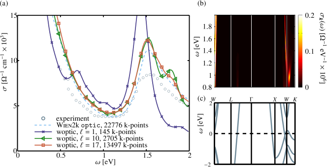
Figure 7: The non-interacting optical conductivity of Al computed by woptic compared to corresponding results from the Wien2k optic package and experimental data [37] in panel (a). For convergence of the uniform Wien2k calculation a large number of (symmetrized) k-points is required, while due to the adaptivity, woptic converges for a much smaller number of k-points. After convergence both programs yield similar results, in particular the experimental peak position is reproduced. (An arbitrary scaling has been applied to the experimental results.) The contributions to the optical conductivity $\sigma$ resolved in $({\boldsymbol{k}},\omega)$-space (b). Only a small part of k-space around $W$ contributes to $\sigma$ and the contributions can be understood by identifying possible transitions in the band structure (c).

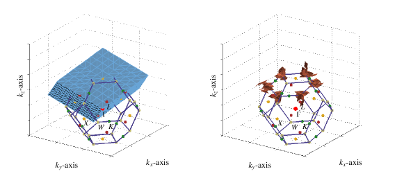
Figure 8: The unsymmetrized initial tetrahedral mesh $\mathcal{T}^{(0)}$ used in the calculations for elementary Al with $3072$ tetrahedra and $4913$ k-points (left). The highly adaptive mesh after $6$ iterations $\mathcal{T}^{(6)}$ with $13152$ tetrahedra and $24667$ k-points (right). For the sake of visualization only the smallest tetrahedra are shown. The region yielding the largest contribution to the estimator (17) is located close to the $W$-point around $[0.7500\quad 0.5000\quad 0.2812]$ in terms of the primitive vectors of the reciprocal unit cell.

As a simple example to show that our adaptive procedure can reproduce standard Wien2k results at much lower computational cost we have chosen fcc-Al. As shown before [20, 38], there is a strong dependency of the optical properties on the quality of the BZ integration. Using a regular grid and the tetrahedron method as implemented in Wien2k’s optic module, up to $20\,000$ k-points in the irreducible wedge of the BZ are necessary to obtain converged results for the optical conductivity. With our adaptive mesh the number of k-points can be greatly reduced. Note that $\sigma(\omega)$ also depends crucially on the applied broadening scheme, and small differences may appear between the two methods, because they are somewhat different in the way the broadening is introduced. The optic module in Wien2k first calculates the imaginary part of the unbroadened dielectric function, $\epsilon_{2}(\omega)$, due to interband transitions and the plasma frequency due to intraband transitions, and adds smearing later (using Lorentzian broadening). On the other hand, the Green’s function method uses a related broadening constant $\delta$ for the self energy $\Sigma(\omega)\equiv-\text{i}\delta$ which enters into the Green’s function (7).

The reason for the slow convergence of $\sigma$ with the number of k-points is quite obvious when one inspects the band structure. Consider the first interband peak at $\omega\approx$1.5\text{\,}\mathrm{eV}$$ (Fig. 7(a)). In the relevant energy range, only a narrow region of the BZ around $W$ contributes, as seen in the k-resolved contributions to $\sigma(\omega)$ (Fig. 7(b)). Comparison with the bandstructure (Fig. 7(c)) shows that these contributions stem from four bands near the Fermi level at $W$ (two particle and two hole bands). A regular mesh must be quite dense to properly sample these small portions of the BZ, while our adaptive scheme is much more efficient. This is illustrated in Fig. 8, where one can see that the regions around the $W$-point are refined most and have the smallest tetrahedra.

5.2 Strontium vanadate

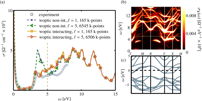
Figure 9: The interacting and non-interacting optical conductivity of SrVO3 computed by the adaptive algorithm woptic (optic mode) compared to experiment [39] in panel (a). While the interacting result is much closer to experiment, the convergence of the algorithm requires far fewer iterations than for Al both in the interacting and in the non-interacting case. This indicates that larger regions of k-space contribute to the optical conductivity, as also suggested by the contributions to $\sigma$ resolved in $({\boldsymbol{k}},\omega)$-space (b). (Note also the different scales of the contributions here and in Fig. 10.) A significant part of the optical conductivity in the energy window under investigation stems from O-$p\rightarrow$V-d transitions, which can be understood by inspection of the band structure (c). In panels (a) and (b), the dashed line indicates the restricted frequency window ($0$ to $5\text{\,}\mathrm{eV}$), which has been considered for the illustration of the evolution of the tetrahedral mesh in Fig. 10. In the non-interacting case, the broadening, in particular the finite width of the Drude peak, arises solely from the small imaginary self energy $\Sigma=-\text{i}\delta$ which is added for this purpose. By contrast, in the interacting case, it is a direct result of DMFT.

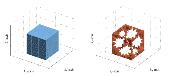
Figure 10: The unsymmetrized initial tetrahedral mesh $\mathcal{T}^{(0)}$ used in the non-interacting calculations for SrVO3 with $3072$ tetrahedra and $4913$ k-points (left). After $5$ iterations, in the highly adaptive mesh regime ($\theta=0.9$), the mesh $\mathcal{T}^{(5)}$ has $4920$ elements and $9533$ k-points (right); for the sake of visualization only the smallest tetrahedra are shown)

As a second application of the method, we present in this section calculations for SrVO3. Its low-energy electronic structure is dominated by the degenerate $3$d-$\text{t}_{2g}$ orbitals of vanadium and it constitutes a textbook example of a strongly correlated metal, perfectly suited for illustrating the intermediate steps and the final results of the woptic package. Specific details about the crystal and electronic structures of SrVO3 can be found, e.g., in Refs. [26, 32]. In fact, SrVO3 is a good example of a situation where DFT cannot accurately describe the low-energy optical response of the system, necessitating the inclusion of local correlation effects, e.g. by means of DMFT. In this work, we focus on the workings of the adaptive algorithm rather than physical implications of our results; see Ref. [26] for a discussion about the latter.

In Fig. 9, the intermediate ($\ell=1$) and final ($\ell=5$) results for the optical conductivity of SrVO3 are reported, in each case for an interacting and a non-interacting calculation. Experimental results from Ref. [39] are reproduced for comparison. Here, the DMFT calculations have been performed using a Kanamori interaction [42] with parameters $U=$5.05\text{\,}\mathrm{eV}$$, $U^{\prime}=$3.55\text{\,}\mathrm{eV}$$ and $J=$0.75\text{\,}\mathrm{eV}$$, consistent with the setup used in Ref. [26]. Since the random-gauge problem is absent in this case due to the cubic symmetry (see Sec. 4), we use optic mode for the interacting optical conductivity. One immediately notes the role of the electronic correlations, as evidenced by a significant shift of optical spectral weight from the Drude peak and the frequency window between $3$ and $5\text{\,}\mathrm{eV}$ to higher energies as compared to the non-interacting calculations. Such many-body effects are expected due to the correlated nature of the $3$d-$\text{t}_{2g}$ orbitals of SrVO3, and they significantly improve the match between theory and experiment.

A more detailed analysis of the woptic results in Fig. 9 shows that the convergence of the adaptive algorithm is much faster than for the Al case of the previous section. This can be understood by plotting the k-resolved contributions to $\sigma(\omega)$ (i.e., the integrand of the k-summation of Eq. 4), as shown in Fig. 9(b): In the wide energy range considered (i.e., up to $15\text{\,}\mathrm{eV}$), the contributions to the optical conductivity are spread over all of k-space. As a consequence, the adaptivity of the woptic algorithm becomes less important and the final adaptive mesh (not shown) essentially coincides with one obtained in a uniform calculation. This would be different when focusing on the low-energy region (e.g., up to $5\text{\,}\mathrm{eV}$ as marked by the dashed lines in Fig. 9) – as is usual when comparing with optical spectroscopic experiments. In that case, the predominant contribution to $\sigma(\omega)$ below $5\text{\,}\mathrm{eV}$ (apart from the Drude peak) is from around the $\Gamma$ point, and between $\Gamma$ and $X$. This corresponds to the peak in $\sigma(\omega)$ located at about $4\text{\,}\mathrm{eV}$ in the non-interacting spectrum, which originates not from optical transitions within the V-$\text{t}_{2g}$ orbitals, but rather from transitions between the O-$2p$ and the V-$\text{e}_{g}$ bands.

This situation is well reflected in the evolution of the tetrahedral mesh, reported in Fig. 10 for a calculation in the window up to $5\text{\,}\mathrm{eV}$, and performed with a highly adaptive mesh ($\theta=0.9$) for the sake of illustration. In the right panel of Fig. 10 the resulting tetrahedral mesh after $5$ iterations is visualized, showing refinements essentially from $\Gamma\rightarrow X$, which is exactly the region we identified in Fig. 9(b) and (c). Moreover, especially along this k-path, the p and the $\text{e}_{g}$ orbitals mainly responsible for the optical transitions are relatively flat and hence difficult to resolve in $({\boldsymbol{k}},\omega)$-space, which explains woptic’s behavior in this case.

6 Summary

We have developed a flexible and efficient adaptive BZ integration algorithm based on a recursively generated tetrahedral k-mesh. In regions where the numerical error would otherwise be large, the k-mesh becomes fine, whereas it remains coarser elsewhere. We apply this approach to the optical conductivity in a Wannier basis, with the possibility to include a many-body self energy $\Sigma(\omega)$ on top of the DFT band structure. The peakedness of the contributions in k-space is determined mainly by the band structure and by the imaginary part of the self energy, which broadens the peaks. Thus, weakly interacting materials, where $\Im\Sigma$ is small, tend to have more sharply peaked contributions.

Results for Al and SrVO3 illustrate the algorithm and its performance. These calculations would require much more computational effort using uniform k-grids.

The woptic package, our implementation of the adaptive k-mesh algorithm in the framework of Wien2k, Wannier90, and DMFT, is available at http://woptic.github.io. In addition to the ready-made computation of the optical conductivity, dc conductivity, and thermopower, the k-mesh management code may easily be adapted to other quantities, in particular where a conventional tetrahedron integration is impossible or impractical.

In order to include transitions involving bands beyond the Wannier projection, an outer band window may be defined, although this leads to certain numerical problems in some cases (see Sec. 4). The outer bands will be described at the DFT level, i.e. without a self energy. Apart from the physical, k-integrated quantities, woptic also provides tools to examine the k-dependent contributions (as in Figs. 7 and 9 (b)), which often provide valuable physical insight.

References

-
[1]
H. J. Monkhorst, J. D. Pack,
Special points for
Brillouin-zone integrations, Phys. Rev. B 13 (12) (1976) 5188–5192.
doi:10.1103/PhysRevB.13.5188.
URL http://link.aps.org/doi/10.1103/PhysRevB.13.5188 -
[2]
D. J. Chadi, M. L. Cohen,
Special Points in
the Brillouin Zone, Phys. Rev. B 8 (12) (1973) 5747–5753.
doi:10.1103/PhysRevB.8.5747.
URL http://link.aps.org/doi/10.1103/PhysRevB.8.5747 -
[3]
D. J. Chadi, Special
points for Brillouin-zone integrations, Phys. Rev. B 16 (4) (1977)
1746–1747.
doi:10.1103/PhysRevB.16.1746.
URL http://link.aps.org/doi/10.1103/PhysRevB.16.1746 -
[4]
P. E. Blöchl, O. Jepsen, O. K. Andersen,
Improved tetrahedron
method for Brillouin-zone integrations, Phys. Rev. B 49 (23) (1994)
16223–16233.
doi:10.1103/PhysRevB.49.16223.
URL http://link.aps.org/doi/10.1103/PhysRevB.49.16223 -
[5]
W. Metzner, D. Vollhardt,
Correlated
Lattice Fermions in Dimensions, Phys. Rev. Lett. 62 (3)
(1989) 324–327.
doi:10.1103/PhysRevLett.62.324.
URL http://link.aps.org/doi/10.1103/PhysRevLett.62.324 -
[6]
A. Georges, G. Kotliar,
Hubbard model in
infinite dimensions, Phys. Rev. B 45 (12) (1992) 6479–6483.
doi:10.1103/PhysRevB.45.6479.
URL http://link.aps.org/doi/10.1103/PhysRevB.45.6479 -
[7]
G. Kotliar, S. Y. Savrasov, K. Haule, V. S. Oudovenko, O. Parcollet, C. A.
Marianetti,
Electronic structure
calculations with dynamical mean-field theory, Rev. Mod. Phys. 78 (3) (2006)
865–951.
doi:10.1103/RevModPhys.78.865.
URL http://link.aps.org/doi/10.1103/RevModPhys.78.865 -
[8]
K. Held, Electronic structure
calculations using dynamical mean field theory, Adv. Phys. 56 (6) (2007)
829–926.
URL http://arxiv.org/abs/cond-mat/0511293 -
[9]
J. P. Perdew, K. Burke, M. Ernzerhof,
Generalized
Gradient Approximation Made Simple, Phys. Rev. Lett. 77 (18) (1996)
3865–3868.
doi:10.1103/PhysRevLett.77.3865.
URL http://link.aps.org/doi/10.1103/PhysRevLett.77.3865 -
[10]
P. Blaha, K. Schwarz, P. Sorantin, S. Trickey,
Full-potential,
linearized augmented plane wave programs for crystalline systems, Computer
Physics Communications 59 (2) (1990) 399–415.
doi:10.1016/0010-4655(90)90187-6.
URL http://www.sciencedirect.com/science/article/pii/0010465590901876 -
[11]
J. Kuneš, R. Arita, P. Wissgott, A. Toschi, H. Ikeda, K. Held,
Wien2wannier:
From linearized augmented plane waves to maximally localized Wannier
functions, Computer Physics Communications 181 (11) (2010) 1888–1895.
doi:10.1016/j.cpc.2010.08.005.
URL http://www.sciencedirect.com/science/article/pii/S0010465510002948 -
[12]
A. A. Mostofi, J. R. Yates, Y.-S. Lee, I. Souza, D. Vanderbilt, N. Marzari,
wannier90:
A tool for obtaining maximally-localised Wannier functions, Computer
Physics Communications 178 (9) (2008) 685–699.
doi:10.1016/j.cpc.2007.11.016.
URL http://www.sciencedirect.com/science/article/pii/S0010465507004936 -
[13]
L. Hedin, New Method
for Calculating the One-Particle Green’s Function with
Application to the Electron-Gas Problem, Phys. Rev. 139 (3A) (1965)
A796–A823.
doi:10.1103/PhysRev.139.A796.
URL http://link.aps.org/doi/10.1103/PhysRev.139.A796 -
[14]
J. M. Tomczak, M. Casula, T. Miyake, F. Aryasetiawan, S. Biermann,
Combined
GW and dynamical mean-field theory: Dynamical screening effects in
transition metal oxides, EPL (Europhysics Letters) 100 (6) (2012) 67001.
doi:10.1209/0295-5075/100/67001.
URL http://stacks.iop.org/0295-5075/100/i=6/a=67001?key=crossref.6924fb4a403bf2fbd800c92cb62524db -
[15]
A. Toschi, A. A. Katanin, K. Held,
Dynamical vertex
approximation: A step beyond dynamical mean-field theory, Phys. Rev. B
75 (4) (2007) 045118.
doi:10.1103/PhysRevB.75.045118.
URL http://link.aps.org/doi/10.1103/PhysRevB.75.045118 -
[16]
A. N. Rubtsov, M. I. Katsnelson, A. I. Lichtenstein,
Dual fermion
approach to nonlocal correlations in the Hubbard model, Phys. Rev. B
77 (3) (2008) 033101.
doi:10.1103/PhysRevB.77.033101.
URL http://link.aps.org/doi/10.1103/PhysRevB.77.033101 -
[17]
T. Maier, M. Jarrell, T. Pruschke, M. H. Hettler,
Quantum cluster
theories, Rev. Mod. Phys. 77 (3) (2005) 1027–1080.
doi:10.1103/RevModPhys.77.1027.
URL http://link.aps.org/doi/10.1103/RevModPhys.77.1027 -
[18]
G. H. Wannier, The
Structure of Electronic Excitation Levels in Insulating
Crystals, Phys. Rev. 52 (3) (1937) 191–197.
doi:10.1103/PhysRev.52.191.
URL http://link.aps.org/doi/10.1103/PhysRev.52.191 -
[19]
N. Marzari, D. Vanderbilt,
Maximally localized
generalized Wannier functions for composite energy bands, Phys. Rev. B
56 (20) (1997) 12847–12865.
doi:10.1103/PhysRevB.56.12847.
URL http://link.aps.org/doi/10.1103/PhysRevB.56.12847 -
[20]
C. Ambrosch-Draxl, J. O. Sofo,
Linear
optical properties of solids within the full-potential linearized augmented
planewave method, Computer Physics Communications 175 (1) (2006) 1–14.
doi:10.1016/j.cpc.2006.03.005.
URL http://www.sciencedirect.com/science/article/pii/S0010465506001299 -
[21]
G. K. H. Madsen, P. Blaha, K. Schwarz, E. Sjöstedt, L. Nordström,
Efficient
linearization of the augmented plane-wave method, Phys. Rev. B 64 (19)
(2001) 195134.
doi:10.1103/PhysRevB.64.195134.
URL http://link.aps.org/doi/10.1103/PhysRevB.64.195134 -
[22]
G. Rohringer, A. Valli, A. Toschi,
Local electronic
correlation at the two-particle level, Phys. Rev. B 86 (12) (2012) 125114.
doi:10.1103/PhysRevB.86.125114.
URL http://link.aps.org/doi/10.1103/PhysRevB.86.125114 -
[23]
A. Toschi, R. Arita, P. Hansmann, G. Sangiovanni, K. Held,
Quantum dynamical
screening of the local magnetic moment in Fe-based superconductors, Phys.
Rev. B 86 (6) (2012) 064411.
doi:10.1103/PhysRevB.86.064411.
URL http://link.aps.org/doi/10.1103/PhysRevB.86.064411 -
[24]
A. Georges, G. Kotliar, W. Krauth, M. J. Rozenberg,
Dynamical mean-field
theory of strongly correlated fermion systems and the limit of infinite
dimensions, Rev. Mod. Phys. 68 (1) (1996) 13.
doi:10.1103/RevModPhys.68.13.
URL http://link.aps.org/doi/10.1103/RevModPhys.68.13 -
[25]
J. M. Tomczak, S. Biermann,
Optical properties
of correlated materials: Generalized Peierls approach and its application
to , Phys. Rev. B 80 (8) (2009) 085117.
doi:10.1103/PhysRevB.80.085117.
URL http://link.aps.org/doi/10.1103/PhysRevB.80.085117 -
[26]
P. Wissgott, J. Kuneš, A. Toschi, K. Held,
Dipole matrix
element approach versus Peierls approximation for optical conductivity,
Phys. Rev. B 85 (20) (2012) 205133.
doi:10.1103/PhysRevB.85.205133.
URL http://link.aps.org/doi/10.1103/PhysRevB.85.205133 -
[27]
J. Bey, Tetrahedral
grid refinement, Computing 55 (4) (1995) 355–378.
doi:10.1007/BF02238487.
URL http://link.springer.com/article/10.1007/BF02238487 -
[28]
M. Ong, Uniform
Refinement of a Tetrahedron, SIAM J. Sci. Comput. 15 (5) (1994)
1134–1144.
doi:10.1137/0915070.
URL http://epubs.siam.org/doi/abs/10.1137/0915070 -
[29]
L. Endres, P. Krysl,
Octasection-based
refinement of finite element approximations of tetrahedral meshes that
guarantees shape quality, Int. J. Numer. Meth. Engng. 59 (1) (2004) 69–82.
doi:10.1002/nme.863.
URL http://onlinelibrary.wiley.com/doi/10.1002/nme.863/abstract - [30] P. Wissgott, A space-time adaptive algorithm for linear parabolic problems, Master’s Thesis, Technische Universität Wien, Vienna, Austria (2007).
-
[31]
P. Deuflhard, A. Hohmann,
Numerical
Analysis in Modern Scientific Computing, Vol. 43 of Texts in
Applied Mathematics, Springer New York, New York, NY, 2003.
URL http://link.springer.com/10.1007/978-0-387-21584-6 - [32] P. Wissgott, Transport Properties of Correlated Materials from First Principles, PhD thesis, Technische Universität Wien, Vienna, Austria (2012).
-
[33]
J. R. Yates, X. Wang, D. Vanderbilt, I. Souza,
Spectral and
Fermi surface properties from Wannier interpolation, Phys. Rev. B
75 (19) (2007) 195121.
doi:10.1103/PhysRevB.75.195121.
URL http://link.aps.org/doi/10.1103/PhysRevB.75.195121 -
[34]
X. Wang, J. R. Yates, I. Souza, D. Vanderbilt,
Ab
initio calculation of the anomalous Hall conductivity by Wannier
interpolation, Phys. Rev. B 74 (19) (2006) 195118.
doi:10.1103/PhysRevB.74.195118.
URL http://link.aps.org/doi/10.1103/PhysRevB.74.195118 - [35] E. Assmann, Spectral properties of strongly correlated materials, PhD thesis, Technische Universität Wien, Vienna, Austria (2015), the chapter relevant for woptic is available at http://www.ifp.tuwien.ac.at/forschung/arbeitsgruppen/cms/software-download/woptic.
-
[36]
I. Souza, N. Marzari, D. Vanderbilt,
Maximally localized
Wannier functions for entangled energy bands, Phys. Rev. B 65 (3) (2001)
035109.
doi:10.1103/PhysRevB.65.035109.
URL http://link.aps.org/doi/10.1103/PhysRevB.65.035109 -
[37]
H. Ehrenreich, H. R. Philipp, B. Segall,
Optical Properties
of Aluminum, Phys. Rev. 132 (5) (1963) 1918–1928.
doi:10.1103/PhysRev.132.1918.
URL http://link.aps.org/doi/10.1103/PhysRev.132.1918 -
[38]
K.-H. Lee, K. J. Chang,
First-principles
study of the optical properties and the dielectric response of Al, Phys.
Rev. B 49 (4) (1994) 2362–2367.
doi:10.1103/PhysRevB.49.2362.
URL http://link.aps.org/doi/10.1103/PhysRevB.49.2362 -
[39]
H. Makino, I. H. Inoue, M. J. Rozenberg, I. Hase, Y. Aiura, S. Onari,
Bandwidth control in
a perovskite-type -correlated metal
II.
Optical spectroscopy, Phys. Rev. B 58 (8) (1998) 4384–4393.
doi:10.1103/PhysRevB.58.4384.
URL http://link.aps.org/doi/10.1103/PhysRevB.58.4384 -
[40]
S. Lupi, L. Baldassarre, B. Mansart, A. Perucchi, A. Barinov, P. Dudin,
E. Papalazarou, F. Rodolakis, J.-P. Rueff, J.-P. Itié, S. Ravy,
D. Nicoletti, P. Postorino, P. Hansmann, N. Parragh, A. Toschi,
T. Saha-Dasgupta, O. K. Andersen, G. Sangiovanni, K. Held, M. Marsi,
A
microscopic view on the Mott transition in chromium-doped V2o3, Nat
Commun 1 (2010) 105.
doi:10.1038/ncomms1109.
URL http://www.nature.com/ncomms/journal/v1/n8/full/ncomms1109.html -
[41]
L. Baldassarre, A. Perucchi, D. Nicoletti, A. Toschi, G. Sangiovanni, K. Held,
M. Capone, M. Ortolani, L. Malavasi, M. Marsi, P. Metcalf, P. Postorino,
S. Lupi,
Quasiparticle
evolution and pseudogap formation in
: An infrared spectroscopy study,
Phys. Rev. B 77 (11) (2008) 113107.
doi:10.1103/PhysRevB.77.113107.
URL http://link.aps.org/doi/10.1103/PhysRevB.77.113107 -
[42]
J. Kanamori, Electron
Correlation and Ferromagnetism of Transition Metals, Prog. Theor.
Phys. 30 (3) (1963) 275–289.
doi:10.1143/PTP.30.275.
URL http://ptp.oxfordjournals.org/content/30/3/275