Hybrid synchronization in coupled ultracold atomic gases

Abstract

We study the time evolution of two coupled many-body quantum systems one of which is assumed to be Bose condensed. Specifically, we consider two ultracold atomic clouds each populating two localized single-particle states, i.e. a two-component bosonic Josephson junction. The cold atom cloud can retain its coherence when coupled to the condensate and displays synchronization with the latter, differing from usual entrainment. We term this effect among the ultracold and the condensed clouds as hybrid synchronization. The onset of synchronization, which we observe in the evolution of average properties of both gases when increasing their coupling, is found to be related to the many-body properties of the quantum gas, e.g., condensed fraction, quantum fluctuations of the particle number differences. We discuss the effects of different initial preparations, and the influence of unequal particle numbers for the two clouds, and we explore the dependence on the initial quantum state, e.g. coherent state, squeezed state, and Fock state, finding essentially the same phenomenology in all cases.

I Introduction

Synchronization has been described in physics, chemistry, biology and social behavior Review ; Review2 ; Review4 . It has been extensively studied in classical non-linear dynamical systems Review3 , and chaotic ones Chaos . The same phenomena have been explored recently in quantum systems, e.g. opto-mechanical devices OptMec , damped harmonic oscillators Syn6 ; Zam2 , driven Syn3 and purely dissipative spins Syn4 , and non-linear optical cavities Syn5 . Synchronization can refer to the mutual effect between detuned but otherwise equivalent components adjusting their rhythms (spontaneous synchronization) as, for instance in Refs. Syn6 ; Zam2 ; Syn4 . Otherwise, a slave system can be driven to follow the dynamics of an external source leading to entrainment or driven synchronization, as for instance in Refs. OptMec ; Syn3 . In quantum many-body physics connections between quantum entanglement and mutual synchronization have been discussed in continuous variable systems  Syn6 ; Zam2 ; Syn7 .

Ultracold atomic gases are particularly relevant quantum many-body systems. Since the first experimental production of Bose-Einstein condensates (BEC’s), they have evolved from being a theoretical curiosity to versatile systems potentially useful in a large number of fields lewenstein-book . Identifying the onset of synchronization in these systems and proposing ways in which such phenomena can be characterized both experimentally and theoretically is a significant step forward in our understanding of the dynamical evolution of coupled quantum many-body systems.

Among the most promising applications are those that stem from the macroscopic sizes of the condensates. BECs are fantastic candidates for high accuracy interferometric devices cronin09 ; schaff15 . These devices rely on the high degree of coherence maintained by BECs.

In recent years, experiments with bi-modal ultracold atomic gases have managed to produce entangled ensembles in which the interferometric capabilities can be largely enhanced giova04 ; esteve08 ; gross10 ; riedel10 ; bohnet14 . These improved interferometric properties are directly related to the pseudo-spin squeezing which can be produced using several techniques kita93 ; Bo97 ; julhei12 . One of the main sources of decoherence in BECs are atom-atom interactions which induce dephasing of the different Fock components Lew96 . Several possibilities, notably the generation of squeezed states Bo97 , have been proposed to increase the coherence times and improve the interferometric capabilities, e.g. of the recent Mach-Zehnder proposal berrada13 .

In this paper we describe how decoherence effects due to the atom-atom interaction can be largely suppressed if a quantum many-body system is coupled to a Bose-Einstein condensate. To be more specific, we consider two bosonic Josephson junctions, $a$ and $b$. Subsystem $b$ is taken to be a BEC at all times during the evolution Smerzi97 , while subsystem $a$ is a standard bosonic Josephson junction, i.e. it may fragment during the evolution Milburn97 ; jame05 ; bruno10 . The coupling between $a$ and $b$ is provided by the contact inter-species interaction. Directly related to this improvement in the coherence times of subsystem $a$, is the onset of a hybrid synchronization between $a$ and $b$.

This synchronization is called hybrid because the two coupled atomic samples are in different regimes, one being a BEC described within a classical approximation and the other being a cloud of cold atoms described with a fully quantum formalism. We notice that in the literature the term hybrid synchronization has also been used in other contexts to describe, for instance, synchronization between (classical) chaotic systems persisting despite the difference in some variables hybrid1 or to the co-existence of different kinds of synchronization in composed (classical) systems like cascade-coupled lasers Ref. hybrid2 .

The paper is organized as follows: In Sect. II we introduce the model system, a two species two-site Bose-Hubbard model. Assuming that one of the species is condensed, we construct our mixed quantum-classical description. In Sec. III the coupled dynamics is studied, particularly the onset of hybrid synchronization and its relation to the condensed fraction of subsystem $a$. Finally, in Sec. IV we present our conclusions.

II Model

Let us consider two different kinds of bosons, $a$ and $b$, populating two single-particle states, $L$ and $R$. The main results described in this paper are essentially independent of the nature of the single-particle states. A way to produce them is by trapping ultracold atoms in a spatial double-well potential GO07 ; esteve08 . A different possibility would be to populate two hyperfine states of the atom and couple them linearly as in Ref. zib10 . A solid-state alternative could be provided by extending the experiments in Ref. amo13 to two different kinds of exciton-polaritons.

The interaction between the bosons is assumed to be described by a contact term with strength proportional to the $s-$wave scattering length. For simplicity the bosons are taken to be two different hyperfine states of the same atom, so that the masses of both species $a$ and $b$, is the same. With these simplifications, the many-body, Bose-Hubbard, Hamiltonian for the system reads,

$$\hat{\cal H}=\hat{\cal H}_{a}+\hat{\cal H}_{b}+\hat{\cal H}_{ab}$$ (1)

where

$$\hat{\cal H}_{a} = -J_{a}(\hat{a}^{\dagger}_{L}\hat{a}_{R}+\hat{a}_{L}\hat{a}^{\dagger}_{R})$$

$$+ {U_{a}\over 2}(\hat{n}_{a,L}(\hat{n}_{a,L}-1)+\hat{n}_{a,R}(\hat{n}_{a,R}-1)),$$

$$\hat{\cal H}_{b} = -J_{b}(\hat{b}^{\dagger}_{L}\hat{b}_{R}+\hat{b}_{L}\hat{b}^{\dagger}_{R})$$

$$+ {U_{b}\over 2}\left(\hat{n}_{b,L}(\hat{n}_{b,L}-1)+\hat{n}_{b,R}(\hat{n}_{b,R}-1)\right),$$

$$\hat{\cal H}_{ab} = {U_{ab}\over 2}\left(\hat{n}_{a,L}-\hat{n}_{a,R})(\hat{n}_{b,L}-\hat{n}_{b,R}\right)\,.$$ (2)

$\hat{a}_{L(R)}^{{\dagger}}$$(\hat{a}_{L(R)})$ and $\hat{b}_{L(R)}^{{\dagger}}$$(\hat{b}_{L(R)})$ are creation (annihilation) operators for the $L$ or $R$ modes of $a$ and $b$. The Hamiltonian includes tunneling terms, proportional to $J_{a(b)}$, which the in absence of any interaction induce periodic Rabi oscillations of the populations between the states. The contact interaction translates into terms with strength proportional to $U_{a}$, $U_{b}$, and $U_{ab}$ which gauge the $aa$, $bb$ and $ab$ contact interactions. The coupling between the two gases is solely due to the term proportional to $U_{ab}$, which is an on site interaction between the atoms of the two species. As customary, we introduce the definition of the population imbalance of each species as, $\hat{z}_{a}=(\hat{n}_{a,L}-\hat{n}_{a,R})/N_{a}$ and $\hat{z}_{b}=(\hat{n}_{b,L}-\hat{n}_{b,R})/N_{b}$.

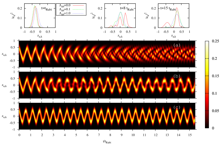
Figure 1: (Color online) Evolution of the distribution of Fock coefficients, $|c_{k}|^{2}$ in Eq. (6) for the quantum gas $a$ as a function of time. We show three different values of the coupling $\Lambda_{ab}=0$ (a), $\Lambda_{ab}=0.1$ (b), and $\Lambda_{ab}=1.0$ (c). The insets depict the distribution $|c_{k}|^{2}$ (linked by a line) for three specific times $t=t_{\rm Rabi}$, $8\,t_{\rm Rabi}$, and $15\,t_{\rm Rabi}$ and the three different couplings. In all cases $N_{a}=N_{b}=30$, $J_{a}=J_{b}=1$ and $\Lambda_{a}=\Lambda_{b}=1$. The initial states are described in the text, $\langle z_{a}\rangle=z_{b}=0.4$ and $\phi_{a}=\phi_{b}=0$. The value of $|c_{k}|^{2}$ (color) is plotted as a function of the imbalance of each Fock state, $z_{a,k}=(2k/N_{a}-1)$, $k=0,\dots,N_{a}$.

The quantum  vardi14 and classical (fully condensed) dynamics Ashhab02 ; diaz09 ; satija09 ; mazzarella10 ; naddeo10 , of this model have been previously studied comparing different dimensional reductions of the three-dimensional equations  mele11 . Also, measure synchronization MS99 has been studied in the classical Tian14 and full quantum case Qiu14 .

II.1 Hybrid, quantum and classical, description of the system

Our main interest is to study the combined evolution of $a$ and $b$. In particular, one of our aims is to discern whether the coupling to a condensed system, $b$, will enhance the degree of condensation of the ultracold gas, $a$. To answer this question, $b$ is assumed to be condensed at all times. Physically, this situation could be attained if the $b$ component has a large enough number of atoms. We thus neglect the quantum fluctuations of the $b$ cloud. In practice this is done by replacing the operators by $c-$numbers, $b_{L}=\sqrt{n_{b,L}}e^{\phi_{b,L}}$, $b_{R}=\sqrt{n_{b,R}}e^{\phi_{b,R}}$. We define the phase difference as $\phi_{b}=\phi_{b,R}-\phi_{b,L}$.

The Hamiltonian is thus written as, $\hat{H}=\hat{\cal H}_{a}+{H}_{b}+\hat{H}_{ab}$, with

$$H_{b} = -2J_{b}\sqrt{n_{b,L}n_{b,R}}\cos\phi_{b}$$

$$+ {U_{b}\over 2}\left(n_{b,L}(n_{b,L}-1)+n_{b,R}(n_{b,R}-1)\right),$$

$$\hat{H}_{ab} = {U_{ab}\over 2}(\hat{n}_{a,L}-\hat{n}_{a,R})(N_{b}z_{b})\,.$$ (3)

where $H_{b}$ is the $c-$number version of $\hat{\cal H}_{b}$. To study the time evolution we solve the following coupled set of equations,

$$i\partial_{t}|\Psi_{a}\rangle = \hat{H}(t)|\Psi_{a}\rangle,$$ (4)

$$\dot{z}_{b} = -2J_{b}\sqrt{1-z_{b}^{2}}\sin\phi_{b},$$

$$\dot{\phi}_{b} = 2J_{b}{\Lambda_{b}}z_{b}+2J_{b}{z_{b}\over\sqrt{1-z_{b}^{2}}}\cos\phi_{b}+2J_{b}\Lambda_{ab}\langle\hat{z}_{a}\rangle(t)\,.$$

where we have introduced the dimensionless ratios, $\Lambda_{a}\equiv N_{a}U_{a}/(2J_{a})$, $\Lambda_{b}\equiv N_{b}U_{b}/(2J_{b})$, and $\Lambda_{ab}\equiv N_{a}U_{ab}/(2J_{b})$.

The time dependence of $\hat{H}$ stems from the time dependence of $z_{b}$ and $\phi_{b}$. This set of equations is obtained considering the $b$ subsystem as a classical parametric driving for the $a$ subsystem and including the feedback effect of $a$ on $b$. Neglecting quantum fluctuations in one field (then classical), still retaining feedback effects due to the interaction with the other (fully quantum), is reminiscent of the ‘time-dependent parametric approximation’ TDPA1 , used to describe large quantum fluctuations in a convectively unstable signal of an optical parametric oscillator, when the pump field is approximated by a classical field while the signal is quantum TDPA2 . Furthermore, here we are neglecting the effect of the quantum fluctuations of $\hat{z}_{a}$ in evaluating the dynamical evolution of $\phi_{b}$, as we approximate $\hat{z}_{a}$ by its expectation value.

The coupled system of Eqs. (4) is solved in the following way. We use a fourth-order Runge-Kutta routine to integrate the differential equation for $z_{b}$ and $\phi_{b}$ coupled to a unitary truncation of the Schrödinger equation for $|\Psi_{a}\rangle$ of the form,

$$|\Psi_{a}(t+\Delta t)\rangle=\left(1+i{\Delta t\over 2\hbar}\hat{H}(t)\right)^{-1}\;\left(1-i{\Delta t\over 2\hbar}\hat{H}(t)\right)\,|\Psi_{a}(t)\rangle\,,$$ (5)

with $\Delta t\approx 0.0002\,t_{\rm Rabi}$.

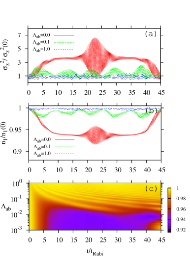
Figure 2: (Color online) Evolution of two relevant many-body properties for different values of the interspecies coupling, $\Lambda_{ab}$. Panels (a) and (b) depict the dispersion of the population imbalance of the $a$ cloud, $\sigma_{z}^{2}$, and the condensed fraction of the $a$ system, $n_{1}$, respectively, for the values considered in Fig. 1, $\Lambda_{ab}=0$, $\Lambda_{ab}=0.1$, and $\Lambda_{ab}=1.0$. Panel (c) scrutinizes the evolution of the condensed fraction for a broader range of values of $0<\Lambda_{ab}<1$. All other parameters are the same as in Fig. 1. Note that the initial condensed fraction, $n_{1}(0)=1$, so that the plotted values are $n_{1}$.

The solutions of Eq. (4) are numerically found to conserve the average energy, $\langle\Psi_{a}|\hat{H}(t)|\Psi_{a}\rangle\simeq\langle\Psi_{a}|\hat{H}(0)|\Psi_{a}\rangle$ in all the calculations reported in this paper. It is worth emphasizing that the coupling between $a$ and $b$ cannot simply be regarded as a driving term for $a$. Conservation of the total average energy implies on average a transfer of energy between the $a$ and $b$ subsystems. The dynamics is thus radically different from the case of a driven single component Josephson junction Driven13 ; Driven10 , which for instance would occur if $z_{b}(t)$ in our description was replaced by a periodic function. In such case, energy would not be conserved and subsystem $a$ would gradually increase its energy. In our formulation the exchange of energy allows for the $mutual$ synchronization of both species and differs from entrainment as will be described in the following section.

Using the Fock basis of the $N_{a}+1$ dimensional space, $|n_{a,L},n_{a,R}\rangle=\{|N_{a},0\rangle,\dots,|0,N_{a}\rangle\}$, the most general $a$ state is written as,

$$|\Psi_{a}\rangle=\sum_{k=0}^{N_{a}}c_{k}\ |k,N_{a}-k\rangle\,.$$ (6)

All many-body properties of the state are computed from the $c_{k}$s, e.g. the average population imbalance of the $a$ cloud reads,

$$\langle\hat{z}_{a}\rangle=\sum_{k=0}^{N_{a}}|c_{k}|^{2}z_{a,k}$$ (7)

with $z_{a,k}=(2k/N_{a}-1)$. The degree of condensation of the cloud is given by its condensed fraction, i.e. the largest eigenvalue, $n_{1}$, of the single-particle density matrix $\rho^{a}(t)$, $\rho_{ij}^{a}(t)={1\over N_{a}}\langle\Psi_{a}(t)|\hat{a}^{\dagger}_{i}\hat{a}_{j}|\Psi_{a}(t)\rangle$, $i,j=L,R$. The condensed fraction is also referred to as single-particle coherence. With this normalization, a fully condensed cloud of $a$ would correspond to $n_{1}=1$ and $n_{2}=0$. In the following sections we discuss the time evolution of $n_{1}$ for different initial conditions and couplings.

III Coupled quantum and condensed dynamics

In this section we will describe how the appearance of synchronization in the combined evolution is found to be directly related to a coherent, in the sense of not dephased, evolution for the $a$ subsystem.

III.1 From dephasing to coherent evolution

Let us first exemplify our discussion with one specific configuration. We will choose as initial state a condensed quantum state for $a$, i.e. all $a$ atoms populate the same single particle state $1/\sqrt{2}(\cos(\theta_{a}/2)a^{\dagger}_{L}+e^{i\phi_{a}}\sin(\theta_{a}/2)a^{\dagger}_{R})|{\rm vac}\rangle$. The many-body state reads,

$$\left|\Psi_{a}(\theta_{a},\phi_{a})\right> = \sum_{k=0}^{N_{a}}\genfrac{(}{)}{0.0pt}{}{N_{a}}{k}^{1/2}[\cos(\theta_{a}/2)]^{k}[\sin(\theta_{a}/2)]^{N_{a}-k}$$ (8)

$$\times e^{i(N_{a}-k)\phi_{a}}|k,N_{a}-k\rangle\;.$$

In particular we will take $\cos(\theta_{a})=\langle\hat{z}_{a}\rangle(t=0)=0.4$ and $\phi_{a}=0$. To emphasize the effect of the coupling term we choose similar conditions for $b$, $z_{b}=0.4$, $\phi_{b}=0$, $N_{a}=N_{b}=30$, $J\equiv J_{a}=J_{b}=1$ and $\Lambda_{a}=\Lambda_{b}=1$. The Rabi time is $t_{\rm Rabi}=\pi/J$, and the Rabi frequency is $\omega_{\rm Rabi}=2\pi/t_{\rm Rabi}=2J$

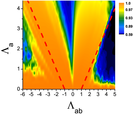
Figure 3: (Color online) Time averaged condensed fraction $\overline{n_{1}}=\int_{0}^{T}n_{1}(t)dt$ with $T=15\,t_{\rm Rabi}$ as a function of $\Lambda_{ab}$ and $\Lambda_{a}=\Lambda_{b}$. The initial condition is again fully condensed for the $a$ component with $\langle z_{a}\rangle(0)=z_{b}(0)=0.4$. All other parameters are as in Fig. 1. The dashed red lines correspond to $1+\Lambda_{a}-\Lambda_{ab}=0$ and $1+\Lambda_{a}+\Lambda_{ab}=0$, see text for details. Notice that the scale in the color bar is nonlinear, and it spans all the values of the data.

In absence of coupling between $a$ and $b$, $\Lambda_{ab}=0$, the quantum system $a$ with a non-zero initial population imbalance evolves with time in a well studied fashion Milburn97 ; jame05 ; bruno10 . Due to the atom-atom interactions which dephase the different Fock components, the initial distribution of $c_{k}$ evolves in time deforming its initial shape (see Fig. 1(a)). For the first oscillations, up to $t\simeq 5\,t_{\rm Rabi}$ the wave packet remains mostly unchanged, which in turn is also reflected in the fact that the $a$ component remains essentially condensed $n_{1}\gtrsim 0.98$ (see Fig. 2(b)). For larger times, $t\gtrsim 10\,t_{\rm Rabi}$, the original shape is lost, the $a$ component is no-longer in a coherent quantum state, and thus the condensed fraction drops below $0.95$. Interaction among atoms $a$ is thus seen to decrease the degree of condensation of the subsystem fairly early. Directly related is the increase in the uncertainty on the particle number difference, $\sigma_{z}^{2}=\langle\hat{z}_{a}^{2}\rangle-\langle\hat{z}_{a}\rangle^{2}$, shown in Fig. 2(a), also appreciable in Fig. 1(a).

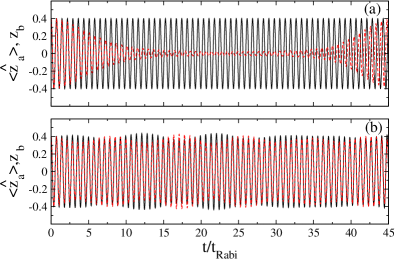
Figure 4: (Color online) Evolution of $\langle\hat{z}_{a}\rangle(t)$ (dashed-red), and $z_{b}(t)$ (solid-black) for two different values of the coupling (a) $\Lambda_{ab}=0$ and (b) $\Lambda_{ab}=0.1$. All other parameters are as in Fig. 1.

When coupling the quantum system $a$ to the condensed one, $b$, a distinctive dynamics is found. The dephasing due to the atom-atom interaction disappears and the quantum system remains condensed for longer times. As seen in Fig. 1(b) for $\Lambda_{ab}=0.1$ the distribution of $|c_{k}|^{2}$ remains closer to a displaced binomial one, which again reflects in a much larger condensed fraction (see Fig. 2 and smaller insets in Fig. 1). Already with this fairly small value of $\Lambda_{ab}$ we find a substantial increase in the condensed fraction, which is now at all times larger than 0.97. Further increasing $\Lambda_{ab}$, the effects are enhanced: The quantum system remains close to condensed for long times, see Fig. 1(c), and the distribution of $|c_{k}|^{2}$ thus evolves, keeping its original shape. The latter is also reflected in $\sigma_{z}^{2}$, see Fig. 2(a), which is found to remain almost constant in the coupled case. Effectively, the coupling to the condensed gas removes the dephasing effects due to the atom-atom interaction, obtaining an almost interaction-free evolution of the quantum system.

This phenomenon is persistent in a broad range of parameters. For $\Lambda_{ab}\gtrsim 0.01$ and maintaining similar initial conditions, the quantum evolution is essentially coherent, as shown in Fig. 2 (b) and  2(c).

Varying the values of $\Lambda_{a}=\Lambda_{b}$ and $\Lambda_{ab}$ one finds the following picture. One can easily prove that within our formalism for $\Lambda_{a}=0$, irrespective of the value of $\Lambda_{ab}$ the condensed fraction of $a$ remains 1. This behavior survives for small values of $\Lambda_{a}\lesssim 0.5$, for which a high degree of condensation for $a$ is also found (see Fig. 3). For $\Lambda_{a}\gtrsim 0.5$, increasing $\Lambda_{ab}$ the condensed fraction of the system is found to remain essentially constant in time (see Fig. 3). Thus, the coupling between $a$ and $b$ increases the coherence of the $a$ system. However, for larger values of $\Lambda_{ab}$, in particular for $\Lambda_{ab}\geq\Lambda_{a}+1$ we observe a decrease of the condensation of $a$ (see Fig. 3). This can be understood from the linear stability analysis of the classical equations around $z_{a},z_{b}\ll 1$. In this case, one of the two natural modes mele11 $\omega_{2}=\omega_{\rm Rabi}\sqrt{1+\Lambda_{a}-\Lambda_{ab}}$ becomes unstable if $\Lambda_{ab}>\Lambda_{a}+1$, which induces decoherence of the $a$ system.

A similar picture is obtained in the attractive interspecies interaction case, $\Lambda_{ab}<0$ (see Fig. 3). In particular, for values of $\Lambda_{a}<4$ we see that increasing the value of $|\Lambda_{ab}|$ the condensation of the $a$ cloud is increased. Further increasing $|\Lambda_{ab}|$, as observed for $\Lambda_{a}\simeq 1.5$, the degree of condensation decreases. The boundary of the classical stability region obtained for small values of the imbalance is found by imposing $\omega_{1}=\omega_{\rm Rabi}\sqrt{1+\Lambda_{a}+\Lambda_{ab}}$ to be real, $\Lambda_{ab}>-\Lambda_{a}-1$.

III.2 Hybrid synchronization

We have described how the coupling between the subsystems prevents the $a$ subsystem from fragmenting during the time evolution for certain coupling values. Now we show how this effect is directly connected to the appearance of synchronization between properties of both subsystems. This synchronization, to which we refer as hybrid, stemming from the hybrid nature of our coupled system, manifests itself in average properties.

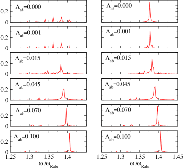
Figure 5: (Color online) Absolute value of the frequency spectrum $z(\omega)$ (Fourier Transform of the average population imbalances), for different values of the coupling $\Lambda_{ab}$. The frequency spectrum of the quantum result, $\langle\hat{z}_{a}\rangle(\omega)$ is given in the left panels. $z_{b}(\omega)$ is depicted in the right panels. The frequency spectra are obtained from time series up to $T_{\rm Max}=585\;t_{\rm Rabi}$.

In the non-coupled case, Fig. 4 (a), the population imbalance of the condensed subsystem, $z_{b}$, is fully periodic Smerzi97 . The frequency seen in the figure, $\omega\simeq 1.38\,\omega_{\rm Rabi}$ is close to the one obtained linearizing around the $z_{b}=0$ fixed point, $\omega=\omega_{\rm Rabi}\,\sqrt{1+\Lambda_{b}}\simeq\omega_{\rm Rabi}\,\sqrt{2}$. The population imbalance of subsystem $a$, $\langle\hat{z}_{a}\rangle$, features characteristic collapses and revivals, which are also present in the condensed fraction and population imbalance dispersion shown in Fig. 2 Milburn97 .

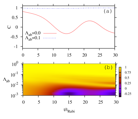
Figure 6: (Color online) Time correlation coefficient $C_{\langle z_{a}\rangle,z_{b}}$ defined in Eq. (9) versus the coupling strength $\Lambda_{ab}$. Panel (a) corresponds to two specific values of $\Lambda_{ab}=0$, $\Lambda_{ab}=0.1$, while (b) contains the time evolution of $C_{<z_{a}>,z_{b}}$ for a broader set of $\Lambda_{ab}$. $\Delta t=14\,t_{Rabi}$. All other parameters are as in Fig. 1.

Coupling both subsystems, Fig. 4 (b), both signals are found to be much more correlated. To quantify this we compare in Fig. 5 the frequency spectra of these signals for different values of $\Lambda_{ab}$. In the uncoupled case the quantum signal is found to have several peaks around the same frequency $\omega\simeq 1.38\,\omega_{\rm Rabi}$. The different equispaced peaks reflect the long evolvent seen in Fig. 4 (upper panel). They arise from the atom-atom interaction which makes the spectrum of the many-body Hamiltonian depart from the equispaced/harmonic case in the uncoupled case producing quantum revivals Milburn97 ; Don04 .

As $\Lambda_{ab}$ is increased, the spread of the peaks in the quantum case is reduced. For $\Lambda_{ab}=0.1$ the Fourier decompositions of both signals are very similar, showing a large peak at $\omega t_{\rm Rabi}\simeq 1.405$. For this value of $\Lambda_{ab}$, $a$ is mostly condensed and the classical description of the full system should approximately hold Ashhab02 ; diaz09 . Indeed, the found frequency is reproduced by the classical equations diaz09 . For this particular case of similar initial conditions of $a$ and $b$, the classical description of the binary mixture predicts, linearizing around $z\ll 1$, just one frequency, $\omega_{1}=\omega_{\rm Rabi}\sqrt{1+\Lambda_{a}+\Lambda_{ab}}=\sqrt{2.1}\,\omega_{\rm Rabi}$ diaz09 . The deviation observed is due to the departure from $z\ll 1$ of our initial conditions $\langle z_{a}\rangle(0)=z_{b}(0)=0.4$.

The synchronization phenomenon, as seen in the Fourier analysis of Fig. 5 goes from several different frequencies for both subsystems in the uncoupled case, to a single major frequency in the coupled case. Thus the two subsystems get frequency-locked as the interaction is increased. It is also worth noting again that in our description subsystem $a$ can also remain condensed, but $b$ is not allowed to fragment. The resulting scenario is that the coupling induces condensation in subsystem $a$.

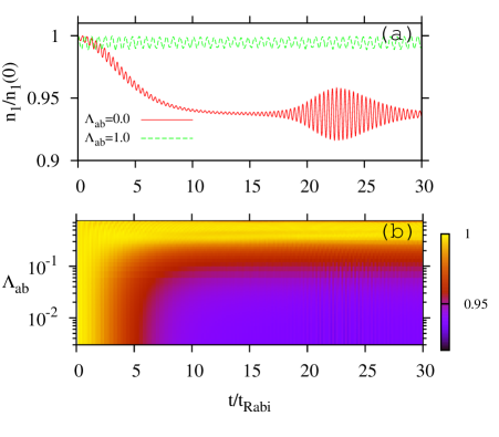
Figure 7: (Color online) Evolution of single particle coherence $n_{1}$ for different values of $\Lambda_{ab}$. With unequal population $\frac{N_{b}}{N_{a}}=10$. In all cases we fixed $\Lambda_{a}=1$, $\Lambda_{b}=10\Lambda_{a}$, and $N_{b}=300$, $N_{a}=30$. The initial state and other parameters are as Fig. 1. (a) corresponds to the two values of $\Lambda_{ab}$. (b) scrutinizes the same function for a more detailed range of values of $0<\Lambda_{ab}<1$.

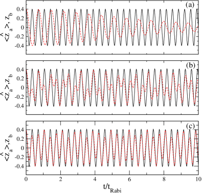
Figure 8: (Color online) Evolution of $\langle\hat{z}_{a}\rangle(t)$ (dashed-red), and $z_{b}(t)$ (solid-black) with $\Lambda_{b}=10\Lambda_{a}$, $\Lambda_{a}=1$, and unequal populations $N_{a}=30$, $N_{b}=300$. Three different values of the coupling are chosen, with (a) $\Lambda_{ab}=0$, (b) $\Lambda_{ab}=0.1$, and (c) $\Lambda_{ab}=0.6$. All other parameters are as in Fig. 7.

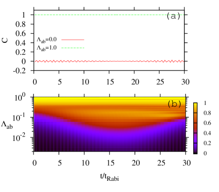
Figure 9: (Color online) Evolution of $C_{\langle z_{a}\rangle,z_{b}}$ for different values of $\Lambda_{ab}$. With unequal population $\frac{N_{b}}{N_{a}}=10$. In all cases we fixed $\Lambda_{a}=1$, $\Lambda_{b}=10\Lambda_{a}$, and $N_{b}=300$, $N_{a}=30$. The initial state and other parameters are as Fig. 1. (a) corresponds to the two values of $\Lambda_{ab}$. (b) scrutinizes the same function for a more detailed range of values of $0<\Lambda_{ab}<1$.

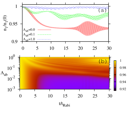
Figure 10: (Color online) Evolution of the condensed fraction of subsystem $a$, $n_{1}$, as a function of time for different values of the coupling $\Lambda_{ab}$. The upper panel corresponds to the three values, $\Lambda_{ab}=0$, $0.1$, and $1.0$. The lower panel scrutinizes the same function for a more detailed range of values of $0<\Lambda_{ab}<1$. Here we consider different initial conditions, $\langle\hat{z}_{a}\rangle(0)=0.4$, and $z_{b}(0)=0.2$.

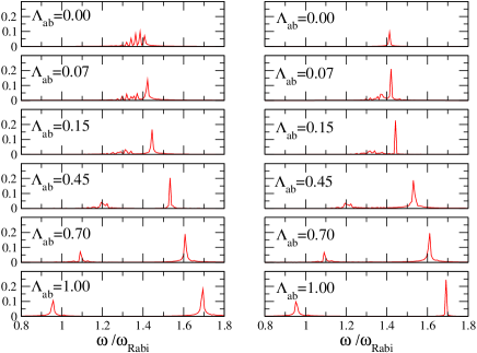
Figure 11: (Color online) Absolute value of the frequency spectrum $z(\omega)$ (Fourier transform of the average population imbalances), for different values of the coupling $\Lambda_{ab}$. Here we consider different initial imbalance in the two subsystems, $\langle\hat{z}_{a}\rangle(0)=0.4$, and $z_{b}(0)=0.1$. The frequency spectrum of the quantum result, $\langle\hat{z}_{a}\rangle(\omega)$ is given in the left panels. $z_{b}(\omega)$ is depicted in right panels. The frequency spectra are obtained from time series up to $T_{\rm Max}=140\,t_{\rm Rabi}$.

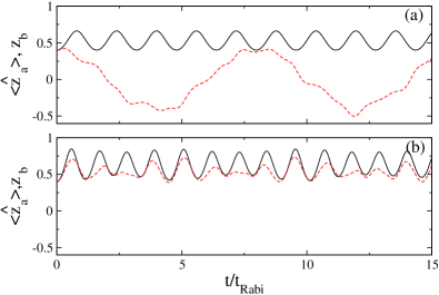
Figure 12: (Color online) Evolution of $\langle\hat{z}_{a}\rangle(t)$ (dashed red), and $z_{b}(t)$ (solid black) for two different values of the coupling (a) $\Lambda_{ab}=0$ and (b) $\Lambda_{ab}=0.2$. The initial conditions are $\langle z_{a}\rangle(0)=z_{b}(0)=0.4$ and $\phi_{a}=\phi_{b}=\pi$ for the $\pi$-phase mode, with $\Lambda_{a}=\Lambda_{b}=1.2$, and $N_{a}=N_{b}=30$.

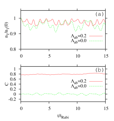
Figure 13: (Color online) Evolution of the condensed fraction of the $a$ system, $n_{1}$ (a), and time correlation coefficient $C_{\langle z_{a}\rangle,z_{b}}$ (b), for the values considered in Fig. 12. The initial condensed fraction, $n_{1}(0)=1$.

In order to have a quantitative characterization of the synchronization, we calculate the time correlation coefficient $C$, which can be used to judge whether two time series are synchronized Syn6 ; Zam2 . For two time signals, $f(t)$ and $g(t)$, it is defined as,

$$C_{f,g}(t,\Delta t)={\overline{\delta f(t)\delta g(t)}\over\sqrt{\overline{\delta f^{2}(t)}\ \overline{\delta g^{2}(t)}}}$$ (9)

where the bar stands for a time average $\overline{f}(t)=\frac{1}{\Delta t}\int_{t}^{t+\Delta t}dt^{\prime}f(t^{\prime})$ with time window $\Delta t$ and $\delta f(t)=f(t)-\overline{f}(t)$. We choose a time window $\Delta t=14\,t_{\rm Rabi}$. For in phase (anti-phase) synchronization $C\sim 1$ ($-1$), while it equals zero for fully non-synchronized cases.

In Fig. 6, we show $C$ as a function of time for different values of the coupling strength $\Lambda_{ab}$. The figure has a similar structure as that found when computing the condensed fraction of the same subsystem in Fig. 2. The subsystem is seen to remain condensed for the same values of $\Lambda_{ab}$ for which the two signals are synchronized.

For $\Lambda_{ab}<0$, we have shown that the results were similar to the $\Lambda_{ab}>0$ case, that is the condensation for the $a$ cloud is enhanced with enough coupling (see Fig. 3). As occurred in the $\Lambda_{ab}>0$ case, the increase in condensation for $\Lambda_{ab}<0$ is also accompanied by an increase in the time correlation function between the average populations of both species, e.g. for $\Lambda_{ab}=-1.0$ with the same parameters and initial conditions as in Fig. 4, $C\sim 1$ is reached.

III.2.1 Effect of unequal populations

The hybrid system we are considering, with $b$ remaining fully coherent during the time evolution, is justified if the number of $b$ atoms is large enough. Up to now we have discussed the case in which $N_{a}=N_{b}$, in order to isolate the effect of the inter-species coupling.

Now, we consider a system with unequal population $N_{b}/N_{a}=10$. With $N_{b}=300$, $N_{a}=30$, and $\Lambda_{b}=10\Lambda_{a}$, $\Lambda_{a}=1$, so that we have $U_{a}=U_{b}$. We keep the initial state and other parameters the same as in Fig. 1. The results show a picture very similar to that of the case with equal populations. In Fig. 7, we show the evolution of single-particle coherence, $n_{1}$, for different values of $\Lambda_{ab}$. We observe an increase of the condensed fraction as $\Lambda_{ab}$ is increased. This is similar to what has been shown in Fig. 2. However, to make a more quantitative comparison of Fig. 2(c) and Fig. 7 (b), we will notice that for the case with unequal populations, in order to reach the same level of single particle coherence as for the case with $N_{a}=N_{b}$, a relatively larger $\Lambda_{ab}$ is needed now.

Fig. 8 shows the hybrid synchronization for this case ($N_{b}\neq N_{a}$). In the non-coupled case, Fig. 8 (a), the population imbalance of the condensed subsystem, $z_{b}$, is fully periodic. Compared with the equal population case, we notice that the frequencies of the two signals are very different. However, by coupling both subsystems with $\Lambda_{ab}=0.1$, as seen in Fig. 8 (b), the signals are found to be more correlated. Further increasing $\Lambda_{ab}$, the two signals show synchronous dynamics due to this coupling effect[Fig. 8 (c)].

To quantify the hybrid synchronization, in Fig. 9 we show the evolution of $C_{\langle z_{a}\rangle,z_{b}}$, for different values of $\Lambda_{ab}$. With $\Lambda_{ab}=0$, Fig. 9(a), the time correlation function is close to zero as expected. With $\Lambda_{ab}=1$, Fig. 9(a), the time correlation function is close to $1$ as hybrid synchronization occurs. By comparing Fig. 9(b) with Fig. 6(b), one sees that in order to reach hybrid synchronization in the case with unequal populations, a larger coupling strength $\Lambda_{ab}$ is needed. This is a general feature of synchronization arising when the coupling between systems is large enough to overcome their detuning. Indeed here the detuning between the two clouds increases with the difference between the populations and needs to be compensated by a larger reciprocal contact interaction.

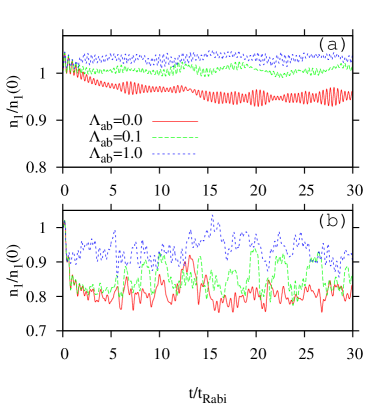
Figure 14: (Color online) Evolution of the condensed fraction of the subsystem as a function of time for three different values of $\Lambda_{ab}$. In the upper panel the initial state is a squeezed state, with an initial condensed fraction $n_{1}(0)=0.9216$. In the lower panel, the initial state is the Fock state, $|21,9\rangle$, which has an average population imbalance of 0.4 and an initial condensed fraction of $21/30=0.7$. All other parameters are the same as in Fig. 1.

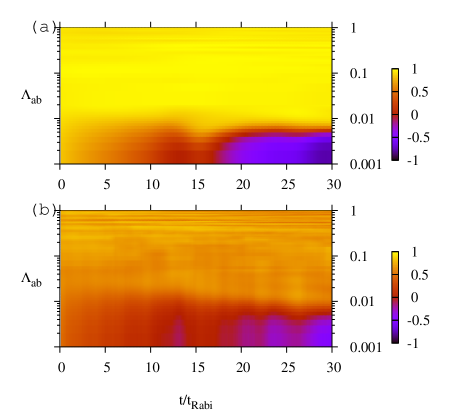
Figure 15: (Color online) Time correlation coefficient $C_{\langle z_{a}\rangle,z_{b}}$ defined in Eq. (9) versus the coupling strength $\Lambda_{ab}$ for the squeezed (upper panel) and Fock (lower panel) cases considered in Fig. 14.

III.2.2 Effects of different initial preparation

Up to now we have considered the same initial population imbalance for $a$ and $b$. Now we consider a more general case, in which the initial average population imbalance is not the same for both subsystems. In particular we will consider $\langle z_{a}\rangle=0.4$ and $z_{b}=0.2$, while all other conditions are as in Fig. 1. The main finding described earlier is again found: Coupling $a$ and $b$ increases the coherence time of subsystem $a$. As described above, the fragmentation of subsystem $a$ which takes place during the uncoupled evolution, see Fig. 10, decreases as the coupling between $a$ and $b$ is increased. For values of $\Lambda_{ab}\simeq\Lambda_{a}=\Lambda_{b}$, $a$ remains almost fully condensed during the evolution.

Let us analyze the Fourier decomposition of the evolution of the population imbalance. Following our previous discussion in the case of decoupled clouds, we find that $z_{b}$ has only one frequency, which now is closer to the one expected in the linear regime, $\omega\simeq\omega_{\rm Rabi}\sqrt{1+\Lambda_{b}}=\sqrt{2}\,\omega_{\rm Rabi}$. The $a$ subsystem, as before has a number of peaks, whose spread is related to the deviation from the equispaced spectrum (which in this case is smaller). As we couple the two subsystems, the spread in the $a$ subsystem disappears and two prominent frequencies appear both for $a$ and $b$. Already for $\Lambda_{ab}=0.45$, we have the same Fourier structure in both cases, signaling the appearance of hybrid synchronization.

The net effect is that for a strong enough coupling both signals oscillate with the same frequency, which is different from the free frequencies. As found in the case of equal initial preparations, the fact that $a$ remains mostly condensed makes a fully classical description of the complete system plausible. Indeed, the two frequencies remaining in the coupled case are reproduced by the classical equations diaz09 . In summary, for different preparation of initial imbalance, it is found that the frequency locking with a single prominent peak appearing as shown in Fig. 5 is replaced by frequency locking of more complex dynamics featuring several spectral components displayed in Fig. 11. This result reminds us of what happens for two coupled classical systems, in which the coupling will induce measure synchronization (MS) Tian14 . In classical MS, the coupled dynamics will exhibit quasi-periodic motions, such that the Fourier analysis of $z_{a}$ and $z_{b}$ shows many peaks rather than one. And in this very special case, the hybrid synchronization is accompanied by MS in the combined dynamics. We emphasize that in general these two phenomena do not need to arise together.

The overall picture as $\Lambda_{ab}$ is varied, see Fig. 10, is similar to the case of equal initial average population imbalance (see Fig. 2). The effect is slightly degraded, finding a lower condensed fraction for similar values of $\Lambda_{ab}$ in the case of different initial average population imbalances. We have also considered different choices of the nonlinearity, i.e., $\Lambda_{a}=2$, $\Lambda_{b}=1$. This has a similar effect as the different preparation of initial imbalances.

Up to now we have only considered hybrid synchronization around stable phase-space points with $\phi=0$. In this case, the classical description of the Josephson junction Smerzi97 shows a single stable minimum for $z=0$ with repulsive interactions. A similar single solution, non-bifurcated, is found for initial preparations $\phi_{a}=\phi_{b}=\pi$ if ($\Lambda_{a}<1,\Lambda_{b}<1$). In this case, we find similar results as those reported above. A more involved situation is found if we consider a bifurcated region of the phase space of each individual Josephson junction, for instance, $\phi=\pi$ and $\Lambda>1$. In this case, the classical description of the junction predicts a self-trapped regime Raghavan . To illustrate this dynamical regime, we have considered the initial condition $\langle z_{a}\rangle(0)=z_{b}(0)=0.4$ and $\phi_{a}=\phi_{b}=\pi$, with $\Lambda_{a}=\Lambda_{b}=1.2$, such that the classical description of each junction (uncoupled) would predict a self-trapped regime. In the non-coupled case, see Fig. 12 (a), the population imbalance of the condensed subsystem, $z_{b}$, is fully periodic and self-trapped. The population imbalance of subsystem $a$, $\langle\hat{z}_{a}\rangle$, features a much more complicated dynamics with no self-trapping. Coupling both subsystems with $\Lambda_{ab}=0.2$, Fig. 12 (b), both signals are found to be much more correlated. The time correlation coefficient $C_{\langle z_{a}\rangle,z_{b}}$ goes from $\simeq 0$ for the uncoupled case, see Fig. 13(b), to a value close to $0.8$ for the coupled case ($\Lambda_{ab}=0.2$). Simultaneously, the degree of condensation, similarly to the case of the $0$-phase mode discussed above, is found to increase with the coupling between the two systems, although the increase is less notable than in the zero phase case. Furthermore, we have tried different initial conditions for the $\pi$-phase mode in the bifurcated region of the classical phase space, and find out that due to the instability associated with the bifurcation zib10 , the parameter space is much smaller compared with $0$-phase mode in achieving hybrid synchronization.

III.2.3 Initially squeezed and Fock states

In all previous results the initial state considered was a condensed many-body state, i.e. condensed fraction $n_{1}=1$. Thus, the effect we have described up to now is how by coupling the quantum to a condensed system the condensed fraction of the quantum state was found to get closer to 1. For that case, the coupling to the condensed state was thus helping the quantum system to remain coherent during the time evolution.

In this section we broaden the set of initial states to consider squeezed and Fock states. Squeezed states are particularly useful as they can be used to improve the efficiency of interferometers made with ultracold atomic systems kita93 ; gross10 ; riedel10 . In brief what we find is that coupling the quantum system to the condensed one has a similar effect as what was described before, i.e. the coupling mostly prevents the dephasing and thus makes the condensed fraction of the quantum system remain approximately constant with time.

In Fig. 14 we consider similar conditions as in Fig. 1, but with squeezed and Fock initial states. The squeezed initial state is built as, $c_{k}=e^{-\frac{{(k-k_{0})^{2}}}{{2\sigma^{2}}}}/\sqrt{\sigma\sqrt{\pi}},$ where $k_{0}$ sets the value of the population imbalance and $\sigma$ sets the squeezing of the state. The coherent state considered above has $\sigma=\sqrt{N_{a}/2}$. A smaller value of $\sigma$ provides a squeezed initial state. In the figure we have taken $\sigma=1$. The picture is very similar to the case of an initial coherent state. Increasing the coupling between the condensed and quantum subsystems the condensed fraction is seen to remain closer to its initial value (not $1$ in this case).

For an initial Fock state, the behavior is similar and the condensed fraction remains closer to its initial value for large enough couplings (Fig. 14, lower panel). The initial state is in this case the Fock state $|21,9\rangle$($c_{k}=\delta_{k,21}$), with $\langle z_{a}\rangle(0)=0.4$.

Finally, in Fig. 15 we present the time correlation for both the squeezed and Fock states used in Fig. 14. For the squeezed case, the picture is similar to the case of an initial coherent preparation. The two subsystems get correlated for $\Lambda_{ab}\geq 0.01$. In the Fock regime, the picture clearly degrades, and although a certain synchronization is found, it does not abide in time.

IV Conclusion

We have considered the coupled dynamics of two ultracold atomic clouds, one of which is assumed to be Bose-Einstein condensed during the evolution. Our main finding is that by increasing the coupling between the two subsystems two net effects take place: (1) the dephasing produced by atom-atom interactions in the non condensed subsystem is found to decrease as the coupling is increased, and (2) the coherent oscillations of both subsystems are found to synchronize. This phase-locking phenomenon is characterized by studying the evolution of the average population imbalance of each subsystem under different conditions. When synchronization appears, the $a$ state is prevented to fragment and remains Bose-Einstein condensed: this allows a comparison of the reported phase-locking with MS within a classical description. Even if the role of the condensate is dominant, preventing the ultracold cloud from losing coherence, the reported synchronization differs from entrainment. The ultracold cloud is indeed $driven$ by the condensate but the latter is also influenced by the feedback of the cloud and both systems evolve towards a different oscillatory dynamics. Synchronization is therefore $hybrid$ (between a condensate driving the ultracold cloud to remain coherent) but $mutual$, being the dynamics of both clouds determined by the reciprocal coupling and in spite of their different regime.

Our results are of relevance for future applications of bimodal quantum many-body systems. In particular, since the dephasing arising from the atom-atom interactions is found to disappear for large enough coupling, we have a way to prevent quantum many-body systems from dephasing. Thus, the relevant properties stored in the system, such as a large squeezing parameter or a large degree of condensation, are preserved during the time evolution if the system is coupled to a condensed one. The hybrid synchronization described, which appears together with the coherent evolution, can be used as an observable control parameter for the phase coherent evolution.

- (1) Y. Kuramoto, Chemical Oscillations, Waves and Turbulence (Springer, Berlin) (1984).
- (2) Z. Néda, E. Ravasz, Y. Brechet, T. Vicsek, and A.-L. Barabási, Nature 403, 849 (2000); D. J. Watts and S.H. Strogatz, Nature 393 440 (1998).
- (3) A. Arenas, A. Díaz-Guilera, J. Kurths, Y. Moreno, and C. Zhou, Phys. Rep. 469 (3), 93 (2008).
- (4) A. Pikovsky, H. Rosenblum, and J. Kurths, Synchronization. A Universal Concept in Nonlinear Sciences (Cambridge University Press, Cambridge, England) (2001).
- (5) L. M. Pecora and T. L. Carroll, Phys. Rev. Lett. 64, 821 (1990). S. C. Manrubia, A. S. Mikhailov, and D. H. Zanette, Emergence of Dynamical Order. Synchronization Phenomena in Complex Systems Lecture Notes in Complex Systems (World Scientic Publishing Co., Singapore) (2004).
- (6) G. L. Giorgi, F. Galve, G. Manzano, P. Colet, and R. Zambrini, Phys. Rev. A 85, 052101 (2012).
- (7) G. Heinrich, M. Ludwig, J. Qian, B. Kubala, and F. Marquardt, Phys. Rev. Lett. 107, 043603 (2011); M. J. Moeckel, D. R. Southworth, E. M. Weig, and F. Marquardt, New J. Phys. 16, 043009 (2014).
- (8) I. Goychuk, J. Casado-Pascual, M. Morillo, J. Lehmann, and P. Hänggi, Phys. Rev. Lett. 97, 210601 (2006); O. V. Zhirov and D. L. Shepelyansky, Phys. Rev. Lett. 100, 014101 (2008); O. Astafiev, K. Inomata, A. O. Niskanen, T. Yamamoto, Yu. A. Pashkin, Y. Nakamura, and J. S. Tsai, Nature (London) 449, 588 (2007).
- (9) P. P. Orth, D. Roosen, W. Hofstetter, and K. LeHur, Phys. Rev. B 82, 144423 (2010); G. L. Giorgi, F. Plastina, G. Francica, and R. Zambrini, Phys. Rev. A 88, 042115 (2013); M. R. Hush, W. B. Li, S. Genway, I. Lesanovsky, and A. D. Armour, Phys. Rev. A 91, 061401(R) (2015).
- (10) T. E. Lee and M. C. Cross, Phys. Rev. A 88, 013834 (2013).
- (11) G. Manzano, F. Galve, G. L. Giorgi, E. Hernández-García, and R. Zambrini, Sci. Rep. 3, 1439 (2013).
- (12) A. Mari, A. Farace, N. Didier, V. Giovannetti, and R. Fazio, Phys. Rev. Lett. 111, 103605 (2013); V. Ameri, M. Eghbali-Arani, A. Mari, A. Farace, F. Kheirandish, V. Giovannetti, and R. Fazio, Phys. Rev. A 91, 012301 (2015).
- (13) M. Lewenstein, A. Sanpera, and V. Ahufinger, Ultracold Atoms in Optical Lattices: Simulating quantum many-body systems, Oxford University Press (2013).
- (14) A. D. Cronin, J. Schmiedmayer, and D. E. Pritchard, Rev. Mod. Phys. 81, 1051 (2009).
- (15) J.-F. Schaff, T. Langen, and J. Schmiedmayer, Riv. Nuovo Cimmento 37, 509 (2014).
- (16) V. Giovnnetti, S. Lloyd, and L. Maccone, Science 306, 1330 (2004).
- (17) J. Esteve, C. Gross, A. Weller, S. Giovanazzi, and M. K. Oberthaler, Nature 455, 1216 (2008).
- (18) C. Gross, T. Zibold, E. Nicklas, J. Estève, and M. K. Oberthaler, Nature 464, 1165 (2010).
- (19) M. F. Riedel, P. Bohi, Y. Li, T. W. Hansch, A. Sinatra, and P. Treutlein, Nature 464, 1170 (2010).
- (20) J. G. Bohnet, K. C. Cox, M. A. Norcia, J. M. Weiner, Z. Chen, and J. K. Thompson, Nat. Photonics 8, 731 (2014).
- (21) M. Kitagawa and M. Ueda, Phys. Rev. A 47, 5138 (1993).
- (22) B. Juliá-Díaz, T. Zibold, M. K. Oberthaler, M. Melé-Messeguer, J. Martorell, and A. Polls, Phys. Rev. A 86, 023615 (2012).
- (23) P. Bouyer and M. A. Kasevich, Phys. Rev. A 56, R1083 (1997); C. Orzel, A. K. Tuchman, M. L. Fenselau, M. Yasuda, and M. A. Kasevich, Science 291, 2386 (2001); W. Li, A. K. Tuchman, H. C. Chien, and M. A. Kasevich, Phys. Rev. Lett. 98, 040402 (2007).
- (24) M. Lewenstein and L. You, Phys. Rev. Lett. 77, 3489 (1996); E. M. Wright, D. F. Walls, and J. C. Garrison, ibid 77, 2158 (1996); A. Imamoglu, M. Lewenstein and L. You, ibid 78, 2511 (1997); J. Javanainen and M. Wilkens, ibid 78, 4675 (1997); Y. Castin and J. Dalibard, Phys. Rev. A 55, 4330 (1997); C. K. Law, H. Pu, N. P. Bigelow and J. H. Eberly, ibid 58, 531 (1998).
- (25) T. Berrada, S. van Frank, R. Bücker, T. Schumm, J.-F. Schaff, J Schmiedmayer, Nat. Commun. 4, 2077 (2013).
- (26) A. Smerzi, S. Fantoni, S. Giovanazzi, and S. R. Shenoy, Phys. Rev. Lett. 79, 4950 (1997).
- (27) S. Raghavan, A. Smerzi, S. Fantoni, and S. R. Shenoy, Phys. Rev. A 59, 620 (1999).
- (28) B. Juliá-Díaz, D. Dagnino, M. Lewenstein, J. Martorell, and A. Polls, Phys. Rev. A 81, 023615 (2010).
- (29) E. Padmanaban, S. Boccaletti, and S. K. Dana, Phys. Rev. E 91, 022920 (2015).
- (30) X. F. Li, W. Pan, B. Luo, and D. Ma, J. Lightwave Tech. 24, 4936 (2006).
- (31) R. Gati and M. K. Oberthaler, J. Phys. B.: At. Mol. Opt. Phys. 40, R61 (2007).
- (32) T. Zibold, E. Nicklas, C. Gross, and M. K. Oberthaler, Phys. Rev. Lett. 105, 204101 (2010).
- (33) M. Abbarchi, A. Amo, V. G. Sala, D. D. Solnyshkov, H. Flayac, L. Ferrier, I. Sagnes, E. Galopin, A. Lemaître, G. Malpuech, and J. Bloch, Nature Physics 9, 275 (2013).
- (34) S. Kumar and C. L. Mehta, Phys. Rev. A 21, 1573 (1980); S. M. Barnett and P. L. Knight, J. Opt. Soc. Am. B 2, 467 (1985).
- (35) R. Zambrini, S. M. Barnett, P. Colet, and M. San Miguel, Phys. Rev. A 65, 023813 (2002).
- (36) M. Heimsoth, D. Hochstuhl, C. E. Creffield, L. D. Carr, and F. Sols, New J. Phys. 15, 103006 (2013).
- (37) E. Boukobza, M. G. Moore, D. Cohen, and A. Vardi, Phys. Rev. Lett. 104, 240402 (2010).
- (38) G. J. Milburn, J. Corney, E. M. Wright, and D. F. Walls, Phys. Rev. A 55, 4318 (1997).
- (39) M. Jääskeläinen, and P. Meystre, Phys. Rev. A 71, 043603 (2005); Phys. Rev. A 73, 013602 (2006).
- (40) R. W. Robinett, Phys. Rep. 392, 1 (2004).
- (41) C. Khripkov and A. Vardi, Phys. Rev. A 89, 053629 (2014).
- (42) S. Ashhab and C. Lobo, Phys. Rev. A. 66, 013609 (2002).
- (43) B. Juliá-Díaz, M. Guilleumas, M. Lewenstein, A. Polls, and A. Sanpera, Phys. Rev. A 80, 023616 (2009).
- (44) I. I. Satija, R. Balakrishnan, P. Naudus, J. Heward, M. Edwards, and C. W. Clark, Phys. Rev. A 79, 033616 (2009).
- (45) G. Mazzarella, M. Moratti, L. Salasnich, and F. Toigo, J. Phys. B: At. Mol. Opt. 43, 065303 (2010).
- (46) A. Naddeo and R. Citro, J. Phys. B: At. Mol. Opt. Phys. 43, 135302 (2010).
- (47) M. Melé-Messeguer, B. Juliá-Díaz, M. Guilleumas, A. Polls, and A. Sanpera, New J. Phys. 13, 033012 (2011).
- (48) A. Hampton and D. H. Zanette, Phys. Rev. Lett. 83, 2179 (1999).
- (49) J. Tian, H. B. Qiu, G. F. Wang, Y Chen, and L. B. Fu, Phys. Rev. E 88, 032906 (2013).
- (50) H. B. Qiu, B. Juliá-Díaz, M. A. García-March, and A. Polls, Phys. Rev. A 90, 033603 (2014).