Study of Calibration of Solar Radio Spectrometers and the quiet-Sun Radio Emission

Abstract

This work presents a systematic investigation of the influence of weather conditions on the calibration errors by using Gaussian fitness, least chi-square linear fitness and wavelet transform to analyze the calibration coefficients from observations of the Chinese Solar Broadband Radio Spectrometers (at frequency bands of 1.0-2.0 GHz, 2.6-3.8 GHz, and 5.2-7.6 GHz) during 1997-2007. We found that calibration coefficients are influenced by the local air temperature. Considering the temperature correction, the calibration error will reduce by about $10\%-20\%$ at 2800 MHz. Based on the above investigation and the calibration corrections, we further study the radio emission of the quiet-Sun by using an appropriate hybrid model of the quiet-Sun atmosphere. The results indicate that the numerical flux of the hybrid model is much closer to the observation flux than that of other ones.

1 Introduction

Broadband radio spectrometers play an important role in observing and revealing the physical processes of the solar atmosphere, solar flares, coronal mass ejections, and other solar activities. When we utilize the data observed by spectrometers to study solar problems, calibration is a key procedure that dominates the reliability of the observational results. At present, there are several solar broadband radio spectrometers running in the world, such as Phoenix at ETH Zurich (100-4000 MHz; Benz et al. (1991)), Ondrejov Radiospectrograph in the Czech Republic (800-5000 MHz; Jiricka et al. (1993)), Brazil Broadband Spectrometer (200-2500 MHz; Sawant et al. (2001)) and the Chinese Solar Broadband Radio Spectrometers (SBRS, 1.10-2.06, 2.60-3.80, and 5.20-7.60 GHz; Fu et al. (1995), Ji et al. (2005)) at the Huairou Solar Observing Station. All the above spectrometers are single-dish telescopes that receive the radio emission of the full solar disk without spatial resolutions. So far, calibration techniques of single-dish radio telescopes can be classified as follows:

(1) Absolute calibration. Skillful practices are needed to determine the absolute calibration values by using an approximate gain of the antenna based on radar and communication techniques, together with an approximate sensitivity derived from experiments with limited accuracy. It is still a difficult problem and usually only applied to polarimeters (Broten & Medd (1960); Findlay (1966); Tanaka et al. (1973); etc).

(2) Relative calibration. This method needs reference emission sources to calculate the emission flux (or brightness temperature). It is usually applied to spectrometers since the absolute calibration of spectrometers would be a huge and very complex mission at broadband frequencies (Messmer et al., 1999).

(3) Nonlinear calibration. When the gain factor of the receiver exceeds its normal range during strong solar radio burst, it is necessary to consider nonlinear calibration (Yan et al., 2002).

Recently, we found that the calibration data has a strong correlation with the local air temperature at frequency of 2.6 - 3.8 GHz of SBRS (Tan et al., 2009). The local air temperature is an important factor that needs to be taken into account in the calibration procedure. We also analyze the impact of the Sun elevation and other weather conditions on the calibration.

Moreover, the calibration of solar radio spectrometers is very important when we compare the observations with theoretical work in the study of the quiet-Sun radio emission. It supplies an accurate flux spectrum, which help us to study the basic nature of the quiet-Sun emission and provide a fundamental knowledge of the solar atmosphere. The radio quiet-Sun has been studied for about 70 yr. Martyn (1946) considered the quiet-Sun as a black body radiation and studied its radio spectrum. He showed the variation of radio brightness across the solar disk at various frequencies and indicated that limb brightening should be observed. Smerd (1950) studied the radio radiation from the quiet-Sun with numerical analysis by applying radiative transfer equations to a typical ray trajectory (Jaeger & Westfold, 1950). He presented a complete analysis of the quiet-Sun radio radiation, and the result is consistent with the observations at wavelengths of 3 cm, 10 cm, 25 cm, 50 cm, 60 cm, 1.5 m & 3.5 m (Pawsey & Yabsley (1949); Christiansen & Hindman (1951)). Since then, more and more observations and studies have been published (Allen (1957); Tanaka et al. (1973); Bastian et al. (1996)). Kundu (1965) reviewed the basic theory of radiative transform and propagation in solar radio astrophysics. Tanaka et al. (1973) used the average value of the daily noon flux to obtain the radio flux spectrum of the quiet-Sun. Other works (Nelson et al. (1985); Zirin et al. (1991)) used the flux density of the quiet-Sun around the minimum of the solar cycle. The numerical computation of the quiet-Sun radio emission has been discussed in those papers (Dulk (1985); Benz (1993); Selhorst et al. (2005)). Benz (2009) pointed out that the radio emission of the quiet-Sun is a well-defined minimum radiation level when the Sun has no sunspots for some weeks. The presence of sunspots enhances the radio emission and produces a slowly variable component. Shibasaki et al. (2011) reviewed radio emission of the quiet-Sun in observations and numerical computation. However, until now few works have paid attention to the study of the totally quiet-Sun radio flux spectrum at centimeter to meter wavelengths. Our work will contribute new observations and computations on this topic by improving the study in several aspects: (1) adopt new flux spectrum observations during solar cycle 23; (2) select the daily noon flux without sunspots $\pm 3$ days as the flux of the quiet-Sun; (3) utilize numerical integration instead of an approximate analytical function in numerical computation of radio emission; (4) use three models (Vernazza et al. (1981); Selhorst et al. (2005); Fontenla et al. (2011)) of the solar atmosphere for comparison of numerical computations. We do not consider the magnetic field $B$ and the scattering effect since the magnetic field $B$ is weak in the quiet-Sun and the scattering effect can be neglected at shorter meter wavelengths (Aubier et al. (1971); Thejappa & MacDowall (2008)).

SBRS has observed the sun since 1994 and accumulated observation data for more than one solar cycle. In this work, we take the observation data of SBRS to analyze the daily calibration and increase the accuracy of the calibration procedure in section 2. Based on the radio flux spectrum of the quiet-Sun, section 3 presents numerical analysis of the quiet-Sun radio emission with improved numerical treatment and several new models of the solar atmosphere. Section 4 gives the main conclusion and some discussions.

2 Observations and Calibration

Three spectrometers of SBRS (Fu et al. 1995, 2004; Ji et al. (2005)) are located at the Huairou Solar Observing Station in China. The first spectrometer (SBRS1) was upgraded three times. SBRS1 observed the Sun and only saved the burst data in the early years. It started routine and calibration observations in 1999 October . It was under construction after 2006 July and started to work again in 2013. The second spectrometer (SBRS2) began to observe the Sun in 1996 September. The third spectrometer (SBRS3) began observing the Sun in 1999 August. SBRS2 and SBRS3 shared the same antenna, with a diameter of 3.2 meter. The main information and performed parameters of SBRS are listed in table 1. During solar cycle 23, the SBRS observed the Sun and did daily calibration at each noon (avoiding the effect of radio bursts), except for the instruments under maintenance. They supply plenty of observations and calibration data to analyze the quiet-Sun radio emission. In this work, we do not consider the daily calibration data in less than 1 yr of observations because small data sets may result in larger error. We only select the daily calibration data from October 1999 to October 2004 of SBRS1, from 1997 to 2007 of SBRS2, and from 2000 to 2007 of SBRS3 except for some big data gaps ($>10days$) or without a noise source or termination (Left panel of Fig.1). We go on analyze the daily calibration data with the daily noon flux from the National Geophysical Data Center (NGDC), and we study some treatments to reduce the calibration errors. At last, the flux spectrum of the quiet-Sun can be obtained from the observing data with calibration.

Table 1: The main information and performance parameters of the component spectrometers

Band	Dm	$f_{re}$	Cadence	Pol	Chan	Observation Period
(GHz)	(m)	(MHz)	(ms)
SBRS1 (1.0-2.0)	7.3	20.0	100	$<$10$\%$	50	1994-2002 Jan
SBRS1 (1.10-2.06)	7.3	4.0	5	$<$10$\%$	240	2002 May-2004 Oct 25
SBRS1 (1.10-1.34)	7.3	4.0	1.25	$<$10$\%$	240	2004 Oct 26-2006 Jul
SBRS1 (1.10-2.10)	7.4	$\sim$2.78	5	$<$10$\%$	360	2013 Aug 20-now
SBRS2 (2.6-3.8)	3.2	10.0	8 or 2∗	$<$10$\%$	120	1996 Sep-now
SBRS3 (5.2-7.6)	3.2	20.0	5 or 1.25∗	$<$10$\%$	120	1999 Aug-now

2.1 Fundamental of Calibration

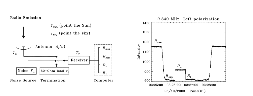
Figure 1: Left panel is the schematic chart of the antenna and receiver system. Right panel is a figuration of the daily calibration data.

Since our data are obtained by broadband spectrometers, this work mainly focus on the relative calibration. The basic principle of the relative calibration was discussed in Messmer et al. (1999) and Yan et al. (2002) in detail. SBRS records a set of calibration data in daily routine observations. The left panel of Fig.1 presents the schematic chart of the antenna and receiver system. The switch may turn to the antenna, noise source, and termination, respectively. Usually, the termination is a 50 ohm resistor. For each case there is an input to the receiver system. $T_{a}$ is equivalent antenna temperature ($T_{a}=T_{sun}$ or $T_{a}=T_{sky}$ when the antenna points to the Sun or the sky, respectively). $T_{n}$ and $T_{t}$ are the equivalent temperature of the noise source and the terminal source, respectively. Therefore, there are four outputs at the computer at various frequencies: the Sun (marked as $R_{sun}$), sky background ($R_{sky}$), noise source ($R_{n}$), and terminal source ($R_{t}$). They are showed in the right panel of Fig.1 by the data processing software. When the gain factor ($Gr$) of the receiver is in the linear range (Yan et al., 2002), they comply with the following relationships:

$$R_{sun}(\nu)=(T_{sun}+T_{r}(\nu))\cdot Gr(\nu)$$ (1)

$$R_{sky}(\nu)=(T_{sky}+T_{r}(\nu))\cdot Gr(\nu)$$ (2)

$$R_{n}(\nu)=(T_{n}(\nu)+T_{r}(\nu))\cdot Gr(\nu)$$ (3)

$$R_{t}(\nu)=(T_{t}(\nu)+T_{r}(\nu))\cdot Gr(\nu)$$ (4)

Here $\nu$ is the observed frequency, and $T_{r}$ is equivalent temperature of the receiver system, which is very small. From Broten & Medd (1960) and Messmer et al. (1999), we have,

$$F_{sun}(\nu)=\frac{2k_{B}\cdot T_{sun}(\nu)}{A_{e}(\nu)}$$ (5)

$F_{sun}$ and $F_{sky}$ are the radio fluxes of the quiet-Sun and sky, respectively. The effective area of the antenna aperture $A_{e}(\nu)$ is changeless and can be considered as a constant. $k_{B}$ is Boltzmann’s constant. The real flux of the sun $F_{0}(\nu)$ should subtract the contribution of the sky $F_{sky}(\nu)$, i.e., equation (6). From equation (1) and (2) we have:

$$F_{0}(\nu)=F_{sun}(\nu)-F_{sky}(\nu)=\frac{2k_{B}}{A_{e}(\nu)}\cdot\frac{R_{sun}(\nu)-R_{sky}(\nu)}{Gr(\nu)}$$ (6)

$Gr(\nu)$ can be deduced with equation (3) and (4). Then equation (6) can be transformed into

$$F_{0}(\nu)=\frac{2k_{B}\cdot(T_{n}(\nu)-T_{t}(\nu))}{A_{e}(\nu)}\cdot\frac{R_{sun}(\nu)-R_{sky}(\nu)}{R_{n}(\nu)-R_{t}(\nu)}$$ (7)

where $R_{sun}(\nu)$, $R_{sky}(\nu)$, $R_{n}(\nu)$ and $R_{t}(\nu)$ are daily calibration data. As written previously, $k_{B}$ and $A_{e}(\nu)$ are constant. $T_{n}$ and $T_{t}$ are equivalent temperatures of the noise source and the terminal source, respectively. The noise source and the terminal source are fixed electronic apparatus and usually stable under the steady environment and no interference. Thus, in equation (8), $C(\nu)$ will be also stable under the steady environment and no interference. It is defined as calibration coefficient

$$C(\nu)=2k_{B}\cdot\frac{(T_{n}(\nu)-T_{t}(\nu))}{A_{e}(\nu)}=F_{0}(\nu)\cdot\frac{R_{n}(\nu)-R_{t}(\nu)}{R_{sun}(\nu)-R_{sky}(\nu)}$$ (8)

For any observed data $R_{sun}(\nu)$ , the corresponding real flux $F_{\odot}(\nu)$ of the Sun is calibrated as follows:

$$F_{\odot}(\nu)=F_{sun}(\nu)-F_{sky}(\nu)=\frac{R_{sun}(\nu)-R_{sky}(\nu)}{R_{n}(\nu)-R_{t}(\nu)}\cdot C(\nu)$$ (9)

Equation (9) is very convenient to do calibration for it does not require that we know the values of $T_{n}(\nu)-T_{t}(\nu)$ and $A_{e}(\nu)$. The bandpass flatness of the spectrum is usually not good for two reasons: 1) the gain factor $Gr(\nu)$ of the receiver varies along frequency; and 2) the antenna system $A_{e}(\nu)$ will also vary more or less along frequency. The calibration with equation (9) will eliminate the frequency property of the gain factor and flat the frequency property of the antenna system with $C(\nu)$ of each frequency. The most important of calibration work is to analyze a suitable calibration coefficient $C(\nu)$ with the right-hand side of expression (8) and reduce the calibration error. Usually we decide the daily noon flux from NGDC as $F_{0}(\nu)$. It can be downloaded from the NGDC Web site, which provides standard flux of solar radio emission at nine fixed frequencies (245, 410, 610, 1415, 2695, 2800, 4995, 8800, 15400MHz). We can calculate flux at any frequency between 245 and 15,400 MHz in using of linear interpolation.

2.2 Impact of the weather in the calibration

Generally, a constant coefficient is adopted in calibration. In practice, the calibration is influenced by the local air temperature more or less. Panels (b) and (c) of Fig.2 show the comparison between the local air temperature and the calibration result at 2800 MHz. Panels (d) and (e) of Fig.2 show that $R_{sun}(\nu)$, $R_{sky}(\nu)$, $R_{n}(\nu)$, and $R_{t}(\nu)$ are all correlated with the local air temperature. From equation (1) and (2) we can deduce that the gain factor $Gr(\nu)$ is influenced by the local air temperature since $T_{sun}(\nu)$ and $T_{sky}(\nu)$ have no relationship with air temperature and $T_{r}(\nu)$ is very small. In fact, the gain factor $Gr(\nu)$ of all bands of SBRS is influenced by the local air temperature more or less. Panels (d) and (e) also show two major jumps (arrows in the figure) at 2001 April 19 and 2002 November 09, respectively. We check the daybook of the observer and find that there is a change to the attenuation of the instrument. Panel (f) shows that the daily calibration coefficients $C_{d}$ are correlated with the local air temperature. The bottom three panels of Fig.2 indicate that the correlation between $C_{d}$ and the local air temperature varied because adjustment of the instrument. We can deduce that ${T_{n}(\nu)-T_{t}(\nu)}$ in equation (8) is also influenced by the local air temperature. All these results imply that the electronic apparatuses of the instruments are influenced by the local air temperature. The relationship between the calibration result (panel (c) of Fig.2) and the humidity (panel (a) of Fig.2) or other weather conditions is not clear. The observation must be stopped when some extreme weather events occur (such as thunder, windstorms, rainstorms and heavy snow). Until now we have found no distinct evidence that the calibration was influenced by normal weather conditions except for air temperature.

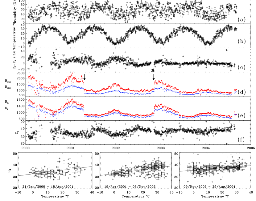
Figure 2: (a and b) Local humidity and local air temperature, respectively; (c) difference between the daily noon flux of SBRS (calibrated with $\overline{C}$) and the daily noon flux from NGDC; (d) $R_{sun}$ (red small cross) and $R_{sky}$ (blue dotted); (e) $R_{n}$ (red small cross) and $R_{t}$ (blue dotted); (f) daily calibration coefficients $C_{d}=F_{0}\cdot\frac{R_{n}-R_{t}}{R_{sun}-R_{sky}}$. The bottom three panels plot the daily calibration coefficients vs. local air temperature for three terms. The sloping line is the least chi-square linear fitness of $C_{d}$ and the local air temperature. All the radio data are at 2800 MHz.

We will explain that the Sun elevation has a small effect on the calibration of this work. Tsuchiya & MacDowall (1965) pointed out that solar flux can be measured without considering the weather condition (atmospheric absorption) at frequency lower than 17 GHz. Considering the atmospheric absorption, the antenna temperature is given by equation as follow.

$$T_{a}=T_{source}e^{-\tau_{0}}+T_{sky}$$ (10)

$$T_{sky}=\int_{0}^{\tau_{0}}T(\tau)e^{-\tau}d{\tau}$$ (11)

$T_{source}$ is the real temperature at the emission source. $T(\tau)$ is the temperature along the line of sight. $\tau$ is the optical depth of the atmospheric absorption.

$$\tau=\int_{h}^{\infty}{\kappa}{\cdot}dh{\cdot}{sec(z)}$$ (12)

where $\kappa$ is the absorption coefficient of the atmosphere. It is small ($<0.006/km$) at frequencies lower than 17 GHz (Tsuchiya & MacDowall, 1965). Moreover, the density of the water vapor and oxygen decreases rapidly along the height of atmosphere $<10km$ above the ground level. The absorption $\kappa$ at the height of $\sim 10km$ will be about $1\%$ of that of the ground level. Here $h$ is height and $z$ is the zenith distance. So the Sun elevation is equal to $90^{o}-z$. The daily calibration observation is done around the noon. The Sun elevation at noon is larger than $26^{o}$, considering that the latitude of Beijing is $40^{o}$. The $sec(z)$ is smaller than 5.8 when the Sun elevation is greater than $10^{o}$. Thus the optical depth in equation (12) is also very small, $\tau_{0}\leq 0.02$. It has only a small effect on the temperature of the emission source.

We also find no distinct evidence that the calibration was influenced by the Sun elevation. If the Sun elevation has a considerable effect on the observation, the following will result: (1) the variation profile of $R_{sun}$(or $R_{sky}$) will show considerable difference from that of $R_{n}$ (or $R_{t}$). The left panel of Fig.1 shows that $R_{n}$ and $R_{t}$ have no relationship with Sun elevation for no connection with antenna; (2) $R_{sun}$(or $R_{sky}$) in summer (high elevation) will be larger than that in winter (low elevation). This is opposite to the observation shown in panel (d) of Fig.2. From all the above analyses, the Sun elevation does not need to be considered in calibration.

We need to understand two problems: (1) the variety of daily calibration data and (2) the relationship between the daily calibration coefficients and the local air temperature. The first is related to the daily calibration data and daily standard flux of solar radio emission. The daily calibration data was recorded by SBRS. They consist of 4 recorded parameters: $R_{sun}$, $R_{sky}$, $R_{n}$, and $R_{t}$ (right panel of Fig.1). The daily noon flux of radio emission at nine fixed frequencies can be downloaded from the NGDC Web site. Usually the observations from Learmonth Observatory are considered since its recording time (05:00 UTC) is very closed to that of SBRS (04:00 UTC). The second problem is related to the local air temperature data of Beijing, which are collected from China Meteorological Administration.

The daily calibration coefficients are calculated by the right-hand side of equation (8) with the daily calibration data of SBRS during 1997 - 2007. There are several steps of pretreatment to exclude the abnormal data: (1) Look up the notebook of the observer, check out the day when the instrument was not in good operation (testing, maintenance, no noise source, etc.), and rule out the data during these cases; (2) get rid of the calibration data with interference, $\pm$NaN value or minus value. The data are wrong and will result in unpredictable errors in the mathematical processing. The main reason for the $\pm$ NaN, minus, and big value of the daily calibration coefficient comes from the electromagnetism interference of the environment. So $R_{sky}$ will be too big or even larger than $R_{sun}$. The relationship between the abnormal data and bad weather conditions is still not clear. We will list all the possible reasons in section 4.

Figure 3: Left: comparison between the average value $\overline{C}$ (long-dashed line) and the gaussian fitness value $\widehat{C}$ (dashed line). Right: difference between the standard deviation of calibration of $\overline{C}$ and that of $\widehat{C}$.

2.3 Analysis of the Calibration

We take an example to analyze the calibration at 2800 MHz. At first, we compare the average value of the daily calibration coefficients ($\overline{C}$) with the Gaussian fitness value of the daily calibration coefficients ($\widehat{C}$) at each frequency. They are $C(\nu)$ in equation (9) when doing calibration. The Gaussian fitness value can exclude the contribution of big or very small values, which usually indicate radio bursts, sunspots or abnormal observations. The left panel of Fig.3 shows the comparison between $\overline{C}$ and $\widehat{C}$ at 2800 MHz. The vertical long-dashed line indicates values of $\overline{C}$. The black solid line is the histogram of the daily calibration coefficient. The dashed line is the Gaussian fitness of the black solid line. The Gaussian fitness is:

$$f(x)=A_{0}e^{\frac{-z^{2}}{2}}+A_{3}+A_{4}x+A_{5}x^{2},z=\frac{x-A_{1}}{A_{2}}$$ (13)

The $x$ value of the maximum $f(x)$ is $\widehat{C}$ marked as vertical dashed line in Fig.3. When $|\overline{C}$-$\widehat{C}|\leq$ 0.02*$\overline{C}$, the average value is close to the gaussian fitness value. This indicates that the observation of this frequency is reliable. In fact, $\overline{C}$ and $\widehat{C}$ are close for most of the frequencies. The most probable value (MPV) is the maximum of the histogram (marked as star in Fig.3). The rms value is the square root of $C_{d}$ (marked as cross in Fig.3). Both the calibration error of the MPV and the rms are lager than those of $\overline{C}$ and $\widehat{C}$. The right panel of Fig.3 shows the comparison between the standard deviation ($\sigma_{av}$) of calibration with $\overline{C}$ and the standard deviation ($\sigma_{G}$) of calibration with $\widehat{C}$. The standard deviation of calibration is calculated by equation (14).

$$\sigma=stddev(F_{H}-F_{N})$$ (14)

Here $F_{H}$ is the daily noon flux calculated by equation (9) with the daily calibration data of SBRS and different $C$ ($\overline{C}$, $\widehat{C}$, etc.). $F_{N}$ is the daily noon flux from NGDC. For $82\%$ of frequencies, $\sigma_{av}$ are greater than $\sigma_{G}$. For the remaining $18\%$ of frequencies, $\sigma_{av}$ are less than or equal to $\sigma_{G}$ because the gaussian fitness deviates from the histogram of the daily calibration coefficients. Thus, $\widehat{C}$ is used as the constant coefficient of calibration. The calibration with a constant coefficient ($\widehat{C}$ or $\overline{C}$) is named the constant calibration.

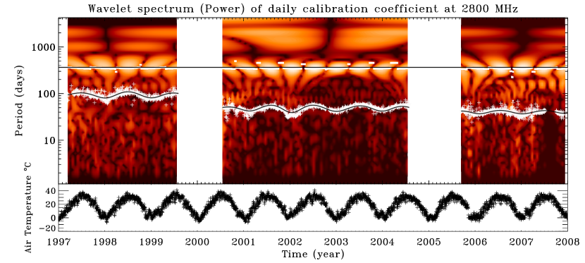
Figure 4: Top: wavelet spectrum of daily calibration coefficients at 2800 MHz. The x-axis is the time (year), and y-axis is the period (days). The white cross is the daily calibration coefficients. The black smooth curve is the calibration coefficients after wavelet filtering. The black solid line shows the period of 365 days. The short white line near the black line of 365 days is the location of maximum power. The data gap represents no observation or during maintenance. Bottom: local air temperature.

The other two sets of calibration coefficients are related to the local air temperature, including calibration coefficients with temperature correction (TC) and temperature-wavelet correction (TWC). Fig.4 shows a strong correlation between the daily calibration coefficients (white cross in top panel) at 2800 MHz and local air temperature (black cross in bottom panel) during 1997 - 2007. Here we partition the data into three terms (1997 - 1999, 2000 - 2004, 2005 - 2007) according to the data gap during which the spectrometers are under maintenance. Those points that exceed the normal range during maintenance should be excluded. Then we decide in equation (15) the linear relationship between the daily calibration coefficients $C_{d}(t)$ and the local air temperature $T_{air}(t)$ for each term. The variable $t$ is the time count in days. $C_{1}$ and $C_{2}$ can be obtained by least chi-square linear fitness between $C_{d}(t)$ and $T_{air}(t)$:

$$C_{d}(t)=C_{1}+C_{2}*T_{air}(t)$$ (15)

Here $C_{1}$ is the first term of the linear fitness. In the second term of the linear fitness, $C_{2}$ is the correct factor that is related to the local air temperature. For each day, the calibration coefficient $C_{TC}=C_{1}+C_{2}*T_{air}$ can be corrected by the local air temperature and replace $C(\nu)$ in equation (9). This is the calibration with temperature correction TC.

TWC is the calibration coefficient corrected by temperature-wavelet analysis. The top panel of Fig.4 plots the power spectrum (red color) of $C_{d}(t)$ after wavelet transform for three terms. The wavelet transform method was discussed by Sych & Yan (2002) in detail. Their work used a complex basis based on the Morlets wavelet which is well localized in both the scale and frequency plane. This makes it possible to rapidly reconstruct the signal even in the presence of a singularity value or in the absence of data. We first transform $C_{d}(t)$ by wavelet to the wavelet data, which are complex numbers and give the power information along the time and period. The period of the maximum power is about 365 days, and the half-power beam widths (HPBWs) are in the range of 260$\sim$530 days. We go on to set the value of the wavelet data beyond the HPBW as zero (that is, we only keep the wavelet data within the HPBWs), and we perform wavelet transform back to new coefficients $\widetilde{C}(t)$. This numerical process is wavelet filtering, which filters out the information we do are not concerned with. The new coefficients $\widetilde{C}(t)$ are plotted as a black smooth curve through $C_{d}(t)$ (white cross). In equation (16), $\widetilde{T}_{air}(t)$ is the local air temperature after wavelet filtering. So, $C_{1}$ and $C_{2}$ can be obtained by least chi-square linear fitness between $\widetilde{C}(t)$ and $\widetilde{T}_{air}(t)$:

$$\widetilde{C}(t)=C_{1}+C_{2}*\widetilde{T}_{air}(t)$$ (16)

$C_{TWC}=C_{1}+C_{2}*T_{air}$ can replace $C(\nu)$ in equation (9) when doing calibration. This is the calibration with TWC.

Figure 5: Each panel plots the daily noon flux of SBRS after $\widehat{C}$ calibration vs. daily noon flux of NGDC. They are plotted as black crosses. The top three panels are the comparison of calibration results with $\widehat{C}$, $C_{TC}$ and $C_{TWC}$ at 2800 MHz. The bottom 11 panels are the yearly calibration results with $\widehat{C}$, $C_{TC}$ and $C_{TWC}$ at 2800 MHz.

We compare the calibration results of three sets of calibration coefficients ($\widehat{C}$, $C_{TC}$ and $C_{TWC}$) at 2800 MHz in both the long term (more than 2 yr) and short term (1 yr). The standard deviations $\sigma_{G}$, $\sigma_{TC}$, and $\sigma_{TWC}$ are of calibration with $\widehat{C}$, $C_{TC}$ and $C_{TWC}$, respectively. They are calculated by equation (14). Each panel of Fig.5 plots the daily noon flux observed by SBRS (calibration with $\widehat{C}$) versus the flux of NGDC. The upper three panels are the calibration results for three long observation terms. The bottom 11 panels show the yearly calibration results. The $\sigma_{TC}$ or $\sigma_{TWC}$ are about $10\%\sim 20\%$ smaller than $\sigma_{G}$ at various observation terms. The difference between $\sigma_{TC}$ and $\sigma_{TWC}$ is small, $\sim 2\%$. In short observation terms, $\sigma_{TC}$ is the smallest. While in long observation terms, $\sigma_{TWC}$ is a little smaller than $\sigma_{TC}$ in most cases. We conclude that TC calibration is better for short observation terms, while TWC calibration is better for long observation terms. The relative standard deviations (RSDs) of calibration with $C_{TC}$ and $C_{TWC}$ are less than $10\%$ in all cases, while RSDs of calibration with $\widehat{C}$ are greater than $10\%$ sometimes because it cannot correct the influence of the air temperature. The RSD of the calibration will be larger when the influence of air temperature is stronger. The $C_{TC}$ of 2007 is used in the calibration during the years of 2008 and 2009. At 2800MHz, $\sigma_{TC}=6.9s.f.u$ is about the same as for the years of 2004 - 2007. In practice, the calibration coefficient $C(\nu)$ should be updated annually.

The daily calibration data of SBRS1 and SBRS3 also have a strong relationship with the local air temperature. The relationship between $C_{d}$ and the local air temperature is quite complex because SBRS1 and SBRS3 were examined and repaired many times. In short observing terms less than 1 yr, there is no significant difference ($<5\%$) between constant calibration and TC (or TWC) calibration. The constant coefficients are used in calibration of them. At the 1.0-2.0 GHz band, the daily noon flux of SBRS1 at 1420 MHz is compared with the daily noon flux of NGDC data at 1415 MHz. The standard deviations are varied within $9\sim 12s.f.u$ in different observation terms. The same is done at 1.10-2.06 GHz band. The standard deviations of calibration are varied within $8\sim 12s.f.u$ at 1420 MHz in different observation terms. At the 5.2-7.6 GHz band, there are no observation data from NGDC. The linear interpolated values between 4995 and 8800 MHz of NGDC are used as comparison. The standard deviations of calibration are varied within $5\sim 18s.f.u$ at 5900 MHz in different observation terms. The observation term with the smallest standard deviation indicates a stable system and few occasional interferences, therefore signifying the best status of the instrument.

2.4 Observation Results

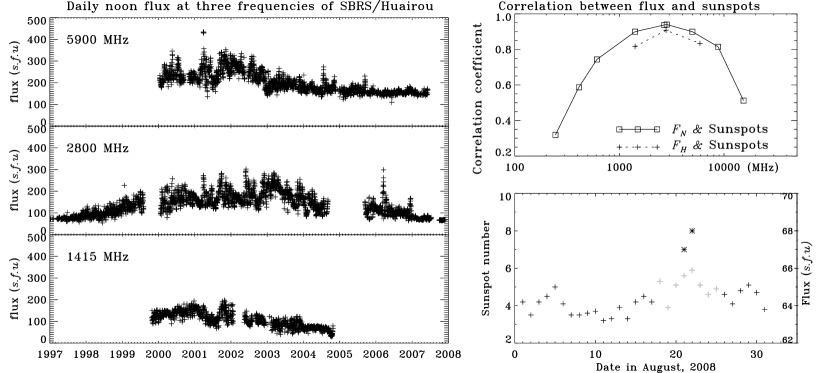
Figure 6: Left: daily noon flux at 1415, 2800, and 5900 MHz observed by SBRS in solar cycle 23. The data gap is without daily calibration or during maintenance. Top right panel: correlation coefficients between the sunspot numbers and the daily noon flux at various frequencies of NGDC and SBRS. Bottom right panel: sunspots numbers (star) and the daily noon flux (cross) at 2800 MHz in 2008 August as an example. The gray cross is excluded because there are sunspots $\pm 3$ days.

The daily noon flux observed by SBRS is calibrated by equation (9) with the calibration coefficient $C(\nu)$. At the 2.6 - 3.8 GHz band, $C(\nu)$ is $C_{TC}$. At other frequency bands, $C(\nu)$ is the constant coefficient. The left panel of Fig.6 plots the daily noon flux at 1415, 2800 and 5900 MHz observed by SBRS during solar cycle 23. In each band of SBRS, we plot the same (or nearby) frequency as nine fixed frequencies of NGDC. The top right panel plots the correlation coefficients between the sunspot numbers and the daily noon flux at various frequencies. The correlation coefficients are consistent with previous works (Christiansen & Hindman, 1951). The bottom right panel plots the sunspot numbers and the daily noon flux at 2800 MHz in 2008 August, as an example. There are still small sunspots or weak active regions during August 21-22 even in the solar minimum. In order to obtain the pure radio flux of the quiet-Sun, we exclude the daily noon flux with sunspots $\pm 3$ days (gray cross in bottom right panel of Fig.6). During the solar minimum period of 2006-2009, 317 days are selected as the candidates. The Gaussian fitness of the daily noon flux of these 317 days is decided as radio flux of the quiet-Sun statistically. They are 55, 67, and 68 sfu at 1415, 2695, and 2800 MHz of SBRS, respectively. The corresponding radio flux of the quiet-Sun from NGDC are 11, 27, 35, 55, 67, 69, 118, 220, and 519 sfu at the nine fixed frequencies, respectively.

3 Theoretical Analysis of the Quiet-Sun Radio Emission

The quiet-Sun radio emission is thermal radiation originated from the ambient plasma in absence of solar activity. The mechanism is bremsstrahlung from electrons interacting with ions in the presence of a relatively weak magnetic field (Shibasaki et al., 2011). In an irregular propagation medium, a wave cannot be represented by a single ray. Small fluctuations in density or magnetic field will distort the incident plane wave as the wave phase propagates at different speeds. Benz (1993) pointed out that the evidence of scattering of solar radio emission is ambiguous, while the scattering hypothesis has been successfully verified for pulsars and irregularities of the interstellar medium. Moreover, other papers (Aubier et al. (1971); Thejappa & MacDowall (2008)) concluded that (1) the scattering effect decreases the intensity of the radio emission and enlarges the size of the radio source, and (2) the scattering effect increases with the radio wavelength ($\propto\lambda^{4}$) and can be neglected at shorter meter wavelengths. We mainly studied the quiet-Sun radio emission at the frequency range of 245 - 15400 MHz in this work; therefore, the scattering effect can be ignored. In numerical analysis of the quiet-Sun radio emission, most previous works are based on the theoretical treatments (Smerd (1950); Dulk (1985); Benz (1993)). The quiet-Sun radio emission is calculated by using equations and treatments as follows.

The radiation transfer equation is

$$\frac{d(I/\mu^{2})}{ds}=\frac{\eta}{\mu^{2}}-\kappa\frac{I}{\mu^{2}}$$ (17)

Here $I$ is the specific intensity of the radiation at frequency of $\nu$; $\eta$ is the volume emissivity, $\kappa$ is the absorption coefficient, and $\mu$ is the refractive index of the medium. The optical depth and the path element have the relationship $d\tau={\kappa}ds$. In this work, the electron temperature $T$ can be treated as uniform in small segments because of the entirely numerical integration. Thus, under conditions of thermodynamic equilibrium in small segment, we have $\eta={\mu^{2}}{\kappa}B(T)$. In the radio frequency band, the Rayleigh-Jeans approximation is $B(T)=\frac{2k_{b}}{c^{2}}{\nu^{2}}T$. Hence, the solution of equation (17) can be obtained:

$$I=\frac{2k_{b}}{c^{2}}\mu^{2}{\nu}^{2}T(1-e^{\tau_{0}-\tau})+I_{0}(\mu/\mu_{0})^{2}e^{\tau_{0}-\tau}$$ (18)

Here the intensity $I_{0}$ and refractive index $\mu_{0}$ are at an optical depth of $\tau_{0}$. $k_{b}$ is the Boltzmann’s constant.

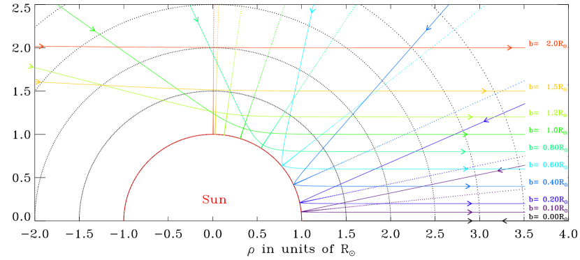
Figure 7: Ray trajectory of 245 MHz in polar coordinates. The bending curves of various colors indicate the ray trajectory of various distances $b$ from the center Sun-Earth line. The normal line of the refraction at the turning point is plotted as a dashed line. The arrow indicate the propagation direction of the ray to the observer.

The ray treatment of radiation (Jaeger & Westfold, 1950) is based on the refraction of the ray path in the solar atmosphere. The equation of the path and the absorption of the rays can be deduced from Snell’s law. Fig.7 shows the ray trajectory in polar coordinates ($\rho,\theta$). Here $\rho=R/R_{\odot}$ is the distance from one point of the ray path to the solar center. These rays will emerge from the solar atmosphere parallel to the observer at a distance $b$ from the center Sun-Earth line. Both $\rho$ and $b$ are in units of the sun’s optical radius $R_{\odot}$ ($6.95\times 10^{10}cm$). The refractive index $\mu$ of an ionized medium decreases with increasing electron density. It follows that a ray passing through the solar atmosphere experiences continuous bending by refraction. The point where the direction of propagation changes from that of decreasing $\mu$ to that of increasing $\mu$ is referred to as the ’reflection point’ or, better, as the turning point. All these rays are calculated with the equation (19) (Jaeger & Westfold, 1950) and the solar atmosphere model in Fontenla et al. (1993, 2011) paper. The path element $ds$ of a trajectory $b$ is given by equation (20)

$$\theta=\int^{\infty}_{\rho}\frac{bd{\rho}}{{\rho}\sqrt{{\mu}^{2}{\rho}^{2}-b^{2}}}$$ (19)

$$ds=R_{\odot}{\sqrt{(d{\rho})^{2}+({\rho}d{\theta})^{2}}}=\frac{R_{\odot}d{\rho}}{\sqrt{1-b^{2}/{{\mu}^{2}{\rho}^{2}}}}$$ (20)

The optical depth can be deduced from the equation of the path (20) and the absorption of the rays. The optical depth between two points ($\rho_{1}$ and $\rho_{2}$) is as follows:

$$\tau_{1,2}(b)=\int^{\rho_{2}}_{\rho_{1}}\frac{{\kappa}R_{\odot}}{\sqrt{1-b^{2}/{\mu^{2}}\rho^{2}}}d\rho$$ (21)

The refractive index is $\mu^{2}\approx{1-(\frac{\omega_{p}}{\omega})^{2}\cdot(1\pm\frac{\Omega_{e}}{\omega}|cos\theta|)^{-1}}\simeq{1-(\frac{\omega_{p}}{\omega})^{2}}$ because the ray frequency is much greater than the local gyrofrequency $\omega\gg\Omega_{e}$ along its propagation in the solar atmosphere of the quiet-Sun (Benz, 1993). The formulae of absorption coefficient $\kappa$ differ in different papers. Some papers (Smerd (1950); Bracewell & Preston (1956); Thejappa & MacDowall (2010)) used $\kappa$ deduced by classical collision theory. The classical collision theory defined the absorption coefficient $\kappa=\frac{\nu_{e,i}}{{\mu}c}(\frac{\omega_{p}}{\omega})^{2}$. Here $\nu_{e,i}$ is the collision frequency of thermal electrons/ions. Some papers (Dulk (1985); Gary et al. (1990)) used $\kappa$ with the Gaunt factor deduced by quantum theory. The formula of $\kappa$ in Dulk (1985) is the same as the approximate analytic formula of Novikov & Thorne (1973); Rybicki & Lightman (1986) at radio wavelength ($\hbar\nu<k_{b}T$). We compare the Gaunt factor value of Dulk (1985) with that of vanHoof et al. (2014) at the solar atmosphere from 100 Mhz to 30 GHz and find that the difference is of $<2\%$ which has a very small impact on the numerical result. Thus in this work we still use the value calculated by the equation of Dulk (1985). Table 2 lists the equations and parameters from different papers. They are all approximatively in the range of $0.15\sim 0.25\frac{N^{2}}{\nu^{2}T^{3/2}\mu}$ under the condition of the solar atmosphere since the classical collision theory is valid and close to the quantum theory when $\hbar\nu\ll k_{b}T$.

Table 2: Parameters of collision frequency $\nu_{e,i}$, average Gaunt Factor $\overline{g}_{ff}(\nu,T)$, and absorption coefficient $\kappa$.

1	2	3	4
Paper	$\nu_{e,i}$ (cgs)	$\overline{g}_{ff}(\nu,T)$	$\kappa$ (cgs)
Smerd (1950)	$\frac{1.36N}{T^{3/2}}ln[1+(\frac{4k_{b}T}{e^{2}N^{1/3}})^{2}]$	-	$\frac{3.65\times 10^{-3}N^{2}}{{\nu}^{2}T^{3/2}\mu}{ln[1+(\frac{4k_{b}T}{e^{2}N^{1/3}})^{2}]}$
Bracewell (1956)	$\frac{1.36N}{T^{3/2}}ln[1+(\frac{4k_{b}T}{e^{2}N^{1/3}})^{2}]$	-	$\sim\frac{0.2N^{2}}{{\nu}^{2}T^{3/2}\mu}$
Dulk (1985)	-	$\frac{\sqrt{3}}{\pi}[18.2+ln(\frac{T^{3/2}}{\nu})]$	$\frac{9.78\times 10^{-3}N^{2}}{{\nu}^{2}T^{3/2}\mu}[18.2+ln(\frac{T^{3/2}}{\nu})]$ $T<2\times 10^{5}$
Dulk (1985)	-	$\frac{\sqrt{3}}{\pi}[24.5+ln(\frac{T}{\nu})]$	$\frac{9.78\times 10^{-3}N^{2}}{{\nu}^{2}T^{3/2}\mu}[24.5+ln(\frac{T}{\nu})]$ $T>2\times 10^{5}$
Thejappa (2010)	$\frac{4.36N}{T^{3/2}}[10.81+ln(\frac{T^{3/2}}{\nu})]$	-	$\frac{2.34\times 10^{-2}N^{2}}{{\nu}^{2}T^{3/2}\mu}[10.81+ln(\frac{T^{3/2}}{\nu})]$ (corona)

From equation (21) and $\kappa$ in Table 2, we have

$$\tau_{1,2}(b)=\frac{9.78\times 10^{-3}R_{\odot}}{\nu^{2}}{\frac{\pi}{\sqrt{3}}}\int^{\rho_{2}}_{\rho_{1}}\frac{{\overline{g}_{ff}(\nu,T)}{N}^{2}}{{T}^{3/2}\sqrt{\mu^{2}-b^{2}/\rho^{2}}}d\rho$$ (22)

$N$ and $T$ are the electron density and electron temperature in the solar atmosphere, respectively. They will be discussed in the next subsection. Equation (22) has a singularity point when $\mu=b/\rho$, $\rho=\rho_{0}$. This point was named the turning point or ’reflection point’ (Smerd (1950); Bracewell & Preston (1956)) where the direction of propagation changes from that of decreasing $\mu$ to that of increasing $\mu$. The appendix proves that the integration is convergent near the singularity point so long as the electron density $N$ increased limitedly and monotonously along the height $\rho$. Therefore, when $\rho>\rho_{0}$, the integration can be calculated with numerical integration.

3.1 The Electron Density and Temperature

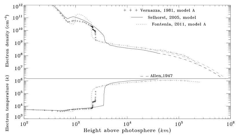
Figure 8: The electron density (top panel) and electron temperature (bottom panel) distribution of different models along the height above photosphere. The classical model Allen (1947) is plotted as long dashed line only at height of higher than $10^{4}km$.

There are many models of the electron density and electron temperature of the quiet-Sun atmosphere. The VAL III model (Vernazza et al., 1981) determined semi-empirical models for six components of the quiet solar chromosphere in using of EUV observations. The series of FAL models (Fontenla et al. 1993, 2009, and 2011) built the semi-empirical models with the optical continuum and EUV/FUV observation. These two models are excellent for reconstructing the optical and ultraviolet observations but still have some discrepancies when describing the radio observations. The discrepancies will be illustrated in the next subsection. Selhorst et al. (2005) proposed a hybrid model that uses the FAL C model (Fontenla et al., 1993) from the photosphere to $1800km$, Zirin et al. (1991) model from $1800$ to $3500km$ in the chromosphere, and Gabriel (1992) model from $3500$ to $40000km$ in the transition region and corona. These three models are selected in this work because the numerical results are not far apart from the observations. Fig.8 shows the electron density and electron temperature distribution of different models along the height above the photosphere. The Fontenla et al. (2011) model is plotted as dashed line. It gave parameters from the chromosphere to the high corona until the height of $\sim 2\times 10^{5}km$. In the higher corona, the electron density is given by the Allen (1947) model as follows:

$$N=10^{8}(1.55\rho^{-6}+2.99\rho^{-16}).cm^{-3}$$ (23)

The Allen model (long-dashed line in Fig.8) will match the value of the Fontenla model at the height of $\sim 2\times 10^{5}km$. The Vernazza model is plotted as a cross in Fig.8. It gave parameters in the chromosphere and transit region until the height of $2439km$. We decide to use the same parameters as the Fontenla model in the corona and the Allen model in the higher corona as before. They are plotted as gray crosses in the figure. The Selhorst model is plotted as a solid line in Fig.8. It gives parameters from the chromosphere to the corona until the height of $3.93\times 10^{4}km$. We decide to use the Allen model after modification (gray long-dashed line in Fig.8) in the higher corona. Then three hybrid models that we used in this work are the FAL+Allen (F+A) model, VAL+FAL+Allen (V+F+A) model, and Selhorst+Allen (S+A) model. For all the models, the electron temperature in the higher corona is equal to the last value given by the corresponding model. We will compare the numerical results of three hybrid models with the observations in the subsection 3.3.

3.2 The Optical Depth and Brightness Temperature across the Solar Disk

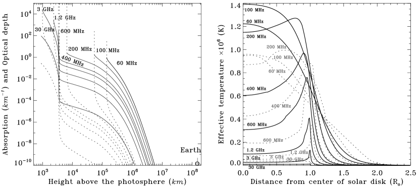
Figure 9: Left panel plots the absorption $\kappa_{n}$ (long dashed line) and the optical depth $\tau_{n,\infty}$ (real line) along the solar height, for each of the central line at eight fixed frequencies. Right panel is the brightness temperature across the solar disk at eight fixed frequencies. Black lines are the numerical result with Selhorst et al. (2005)+ Allen (1947) model. Dashed lines are the results of approximation solution in Smerd (1950).

We do numerical integration entirely in this paper. In equation (22), the optical depth $\tau_{n,n+1}(b)$ is calculated for about 500 points from the turning point (inner limit) to the point after which the contribution is very small (outer limit). The appendix proves that the integration of equation (22) near the turning point is convergent. Beyond the outer limit, the absorption is very small ($<10^{-10}$ $km^{-1}$ in this work) thus, the optical depth can be ignored. The 500 points are decided as follows: (1) the zero point is the turning point $\rho_{0}$; (2) assume the first point $\rho_{1}=\rho_{0}+\Delta\rho_{1}$, $\Delta\rho_{1}\leq 1R_{\odot}$, and calculate the optical depth $\tau_{0,1}$ between the two points; (3) set the midpoint between point 0 and point 1, $\rho_{m}=\rho_{0}+(\rho_{1}-\rho_{0})/2$, and calculate the optical depth of $\tau_{0,m}$ and $\tau_{m,1}$, respectively; (4) if $|\frac{\tau_{0,m}+\tau_{m,1}-\tau_{0,1}}{\tau_{0,1}}|>10^{-2}$, change the midpoint to point 1 and set a new midpoint. Do this circulatory calculation until $|\frac{\tau_{0,m}+\tau_{m,1}-\tau_{0,1}}{\tau_{0,1}}|\leq 10^{-2}$. The calculation error is very small. Then the first point $\rho_{1}=\rho_{m}$ is decided. Usually, the first point is decided as $\Delta\rho_{1}=10^{-12}\sim 10^{-10}R_{\odot}$ by experience. (5) Decide the rest points with this method. It should be taken care that the electron density and electron temperature vary abruptly in the transition region. The step should be $10^{-12}R_{\odot}\leq\Delta\rho_{n}\leq 1.5\times\Delta\rho_{n-1}$ to avoid the big error during calculation. For the points beyond the outer limit, the optical depths are approximated as zero. The left panel of Fig.9 plots the absorption $\kappa_{n}$ and optical depth $\tau_{n,\infty}$ of the central line calculated with the Selhorst + Allen model at eight fixed frequencies as an example. The right panel of Fig.9 shows the brightness temperature (or radiation intensity), which is calculated with equation (18) and (22) for different $b$ at eight fixed frequencies. Black lines are the numerical result of the Selhorst + Allen model in this work. Dashed lines are the result of Smerd (1950) with the approximation solution. It shows differences between two results.

Fig.9 illustrates the main generating region of the quiet-Sun radio emission at varied frequencies. The result is consistent in the main but a little different from the classical results (Smerd (1950); DelaLuz et al. (2010)). At high frequency ($3\sim 30GHz$), the absorption ($<10^{-5}km^{-1}$) and optical depth ($<0.01$) is very small in the corona. The emissivity $\eta={\mu^{2}}{\kappa}B(T)$ are very small in the corona. Thus, the thermal bremsstrahlung emission of the quiet-Sun at high frequency ($3-30GHz$) is mainly produced in the chromosphere. At low frequency ($<300MHz$), the radio emission cannot propagate into the chromosphere. The thermal bremsstrahlung emission of the quiet-Sun at low frequency ($<300MHz$) is mainly produced in the corona. The thermal bremsstrahlung emission of the quiet-Sun at intermediate frequency ($300MHz<\nu<3GHz$) is produced in both the chromosphere and the corona. The limb brightening appears obviously at a frequency range of $200MHz<\nu\leq 30GHz$. The brightness temperature of the solar center radio emission is consistent with the electron temperature of the main generating region.

3.3 Brightness Temperature and Flux Density of the Quiet-Sun

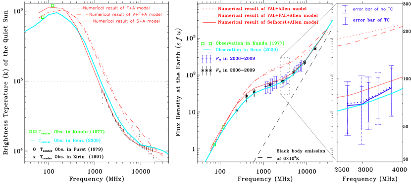
Figure 10: Left: brightness temperature spectrum of the center line of the quiet-Sun. The errors bar are derived from the observations in Zirin et al. (1991). Middle: comparison between numerical results and observations of flux spectrum of the quiet-Sun. The error bars are derived from observations of SBRS and NGDC, respectively. The observation result in Benz (2009) has an accuracy of about 10%. Right: enlargement of a small rectangle from the middle panel. It shows the observation fluxs (thick blue lines) and error bars (thin blue lines) of TC and no TC in the range of 2500-4000 MHz as an example.

We calculate the brightness temperature spectrum and flux spectrum of the quiet-Sun radio emission for three hybrid models (F+A, V+F+A, S+A) at various frequencies. The total amount of radiation per unit time, unit frequency interval, and unit angle from the Sun to a distant observer is given by

$$E=2\pi R_{0}^{2}\int_{0}^{\infty}I(d)d\delta d,$$ (24)

in units of $erg.cm^{-2}Hz^{-1}s^{-1}$. In practice, the upper limit of this integral is replaced by a finite value $d_{p}$, out of which the radiation contribution is very small. The flux density of the quiet-Sun can be transformed with the conversion $1s.f.u=10^{-22}Wm^{2}Hz^{-1}=10^{-19}erg.cm^{-2}Hz^{-1}s^{-1}$. Then we compare the numerical results with observations and find the difference. The left panel of Fig.10 shows the comparison of brightness temperature spectrum between the observations and numerical results of different models. We chosse the observations of Benz (2009) and Zirin et al. (1991) as the standard spectrum because the flux spectrum of Benz (2009) is well consistent with the observations of SBRS-/HSO and NGDC (middle panel of Fig.10). At frequency of $15400MHz$ or nearby, the numerical results of all models and all the observations (Fuerst (1980); Zirin et al. (1991); Benz (2009)) are consistent. This indicates that the parameters in the low chromosphere of all the models fit the observation well. At frequency of $3-10GHz$, the numerical results of the F+A model (mainly Fontenla model) and V+F+A model (mainly Vernazza model) are close to the observations of Fuerst (1980), while the numerical results of the Selhorst+Allen model are close to the observations of Zirin et al. (1991) and Benz (2009). The radio emission at the frequency of $300MHz-3GHz$ comes from the transition region and corona. The numerical results of the Selhorst+Allen model (red solid line) are close to the observations of Benz (cyan solid line) well. Thus, we think that from the transition region to the low corona the parameters of the Selhorst model fit the observations well. It is complex to estimate wether the parameters in the higher corona are good or not owing to a lack of observations at low frequency ($<300MHz$).

Table 3: The center-line brightness temperature and flux density of the quiet-Sun at various frequencies

$\nu[MHz]$	$T_{c}[K]$	$T_{c}[K]$	$T_{c}[K]$	$T_{c}[K]$	$F_{\odot}$	$F_{\odot}$	$F_{\odot}$	$F_{\odot}$	$F_{\odot}$	$F_{\odot}$
	$F+A$	$V+F+A$	$S+A$	$Benz$	$F+A$	$V+F+A$	$S+A$	$Benz$	$F_{N}$	$F_{H}$
245	$1.00\times 10^{6}$	$1.00\times 10^{6}$	$9.69\times 10^{5}$	$7.88\times 10^{5}$	17.3	17.3	15.7	11.2	11
410	$7.93\times 10^{5}$	$7.89\times 10^{5}$	$5.90\times 10^{5}$	$5.50\times 10^{5}$	41.4	21.3	30.3	22.2	27
610	$5.56\times 10^{5}$	$5.27\times 10^{5}$	$2.84\times 10^{5}$	$3.58\times 10^{5}$	69.8	68.9	41.9	32.3	35
1415	$1.68\times 10^{5}$	$1.48\times 10^{5}$	$7.43\times 10^{4}$	$9.70\times 10^{4}$	139	127	60.8	46.9	55	55
2695	$6.21\times 10^{4}$	$5.85\times 10^{4}$	$2.93\times 10^{4}$	$4.19\times 10^{4}$	185	167	77.9	64.7	67	67
2800	$5.76\times 10^{4}$	$5.49\times 10^{4}$	$2.76\times 10^{4}$	$3.68\times 10^{4}$	189	172	80.3	66.8	69	68
4995	$2.74\times 10^{4}$	$3.25\times 10^{4}$	$1.62\times 10^{4}$	$1.88\times 10^{4}$	246	251	121	107	118
8800	$1.49\times 10^{4}$	$2.10\times 10^{4}$	$1.22\times 10^{4}$	$1.38\times 10^{4}$	359	450	233	235	220
15400	$9.46\times 10^{3}$	$1.29\times 10^{4}$	$1.04\times 10^{4}$	$1.16\times 10^{4}$	612	832	562	599	519

The middle panel of Fig.10 plots the flux spectrum of the quiet-Sun radio emission. The quiet-Sun fluxes of SBRS observations (Gaussian fitness value) and the error bars ($3\sigma$) are plotted as blue crosses and short vertical lines. The quiet-Sun fluxes of NGDC (Gaussian fitness value) are plotted as black stars. The NGDC did not present the error of solar flux. Here we use three times the standard deviation ($3\sigma$) of the quiet-Sun data from NGDC as error bars (black short vertical lines). The standard deviation is calculated separately at the low value part and high value part. We find that both the quiet-Sun flux spectra of SBRS and NGDC fit the observation of Benz (cyan solid lines) well. Thus, our work agrees with the brightness temperature spectrum and flux spectrum of Benz (2009) as the standard spectrum of the quiet-Sun radio emission. All the values of brightness temperature and flux density of the quiet-Sun at various frequencies are listed in table LABEL:tbl-2. The right panel of Fig.10 shows the observation flux and error bars of TC (solid blue line) and no TC (dashed blue line) in the range of 2500 - 4000 MHz as an example. It indicates that calibration of TC is more accurate than that of no TC. The red lines are the same numerical results of solar models as in the middle panel of Fig.10. The cyan line is the observation of Benz. As analyzed in subsection 2.3, the difference between TC and TWC calibration is very small ($\sim 2\%$). The observation flux and error bars of TWC are not plotted together.

4 Conclusion and Discussion

SBRS has been observing the Sun and obtaining plentiful data since 1994. This work adopted the observations of SBRS to investigate the calibration procedure and study the quiet-Sun radio emission. The calibration gives accurate observations which is basic and important in the study of the quiet-Sun radio emission, while the study of the quiet-Sun radio emission is a scientific extension of the former part. We first study various impacts to the calibration results and conclude that:

1) Generally, the calibration coefficient is constant and should be upgraded annually. Actually, the calibration result with constant coefficient is found to be related with the local air temperature at all frequency bands of SBRS. One possible reason is that the electronic apparatus of the instruments are influenced by the local air temperature. Thus, the correlation between calibration and local air temperature will vary if there is an adjustment to the instrument.

2) The relationship between calibration results (panel (c) of Fig.2) and the humidity (panel (a) of Fig.2) or other weather conditions is not clear. There is no distinct evidence that the calibration was influenced by normal weather conditions except for air temperature.

3) The Sun elevation has a small effect on the calibration of this work. The absorption of the atmosphere should be considered only when the frequency is higher than 17 GHz (Tsuchiya & MacDowall, 1965) or the Sun elevation is lower than $10^{o}$.

The calibration accuracy is also influenced by the occasional abnormal signal. Some possible reasons for the abnormal signal are listed as follows:

1) Various kinds of interference: wireless communication, plane and airport, satellite, vehicle, lightning, etc. These will result in large values.

2) Unstability of the feed, cable, or noise source.

3) Sometimes, the gain factor may be out of normal range when there is a strong signal (Yan et al., 2002). The beam of the antenna will offset the sun center if the tracking control is out of normal range. These will result in big or saturated values, or small values. The relationship between the abnormal signal and bad weather conditions is still not clear. The calibration with equation (9) will eliminate the frequency property of gain factor $G_{r}(\nu)$, and flatten the frequency property of the antenna system with $C(\nu)$ of each frequency. The calibration with equation (9) does not need the values of $A_{e}(\nu)$ and ${T_{n}(\nu)-T_{t}(\nu)}$.

In order to improve the calibration accuracy, we investigate the influence and properties of the instrument from the data analysis and comparison between different calibration coefficients. All the investigations are under the fundamental of calibration. First, we exclude the abnormal data that are not well observed or are influenced by the interference. Then we compare the calibration results of four sets of calibration coefficients, including average value ($\overline{C}$), the Gaussian fitness value ($\widehat{C}$), constant coefficients after temperature correction ($C_{TC}$), and constant coefficients after temperature-wavelet correction ($C_{TWC}$). The main analysis results are as follows: (1) In the 2.6 - 3.8 GHz band, the calibration errors $\sigma_{G}$ are smaller than $\sigma_{av}$ at $82\%$ of frequencies. Comparing with other constant coefficients of calibration, $\widehat{C}$ is the best. (2) At 2800 MHz, $\sigma_{TC}$ or $\sigma_{TWC}$ are about $10\%-20\%$ smaller than $\sigma_{G}$ at various observation terms. The RSDs of $\sigma_{TC}$ and $\sigma_{TWC}$ are less than $10\%$, while RSDs of $\sigma_{G}$ are greater than $10\%$ sometimes because of the influence of the temperature. The $C_{TC}$ is used in the calibration in the years of 2008 and 2009. The calibration error $\sigma_{TC}=6.9s.f.u$ is about the same as that in the years of 2004 - 2007. (3) The calibrations of SBRS1 and SBRS3 also have a strong relationship with the local air temperature. But there is no significant difference between TC (or TWC) calibration and constant calibration of SBRS1 and SBRS3, which were examined and repaired many times. $\widehat{C}$ is used in the calibration for several short observation terms. The standard deviations of calibration are varied within $8-12s.f.u$ at 1415 MHz and within $5-18s.f.u$ at 5900 MHz for different observation terms, respectively. The observation term with the smallest standard deviation indicates a stable system and few occasional interferences, therefore signifying the best status of the instrument.

The daily noon fluxes of SBRS are calibrated with improved $C(\nu)$. We select the daily noon flux without sunspots $\pm 3$ days as the flux of the quiet-Sun during the solar minimum period of 2006 - 2009. The spectrum of daily noon flux observed by SBRS approaches the spectrum from NGDC well. The daily noon flux is correlated with sunspot numbers. The result is consistent with previous works (Christiansen & Hindman, 1951).

Based on the above investigations, we further study the radio emission from the quiet-Sun. The flux spectrum is strictly the observation without sunspots during the solar minimum period of 2006 - 2009. The numerical simulation of the quiet-Sun radio emission in this work is improved with several semi-empirical solar models and entirely numerical integration instead of approximate solution. The theoretical and treatment has been testified well because it can deduce the same result as that of many papers (Jaeger & Westfold (1950); Thejappa & Kundu (1992); Thejappa & MacDowall (2010); etc). Different works have different treatments, such as (1) different approximations of radiation transformations, (2) different absorption coefficients $\kappa$, (3) consideration of refractive index, scattering effect, or magnetic field. This work uses the radiation transfer equation and bremsstrahlung mechanism of emission without approximation and without scattering effect and magnetic field. The ray treatment of radiation is based on the refraction of the ray path in the solar atmosphere (Jaeger & Westfold, 1950). The refractive index $\mu$ and absorption coefficient $\kappa$ in Dulk (1985) are considered since the Gaunt factor in Dulk (1985) is very close to the numerical value of vanHoof et al. (2014).

The VAL (Vernazza et al., 1981) and FAL (Fontenla et al., 2011) models are excellent for reconstructing the optical and ultraviolet observations but still have some discrepancies in describing the radio observation. Zhang et al. (2001) discuss the discrepancy and attribute the difference to an underestimation of Fe abundance used in the calculation of the UV line emission. Thus, Selhorst et al. (2005) proposed a hybrid model, of which the transition region is about 1000 $km$ higher than in typical VAL and FAL models. We regulate solar models with a combination of different models and compare the numerical results with the observations. The numerical results of the models should be within the confines (error bars) of observations. Finally, we find an appropriate hybrid model that uses the Selhorst model from the chromosphere to the height of $3.93\times 10^{4}km$ above the photosphere and the Allen model in the higher corona. The comparison (Fig.10) between the numerical results and the observations indicates the followings: (1) The numerical results of all models and all observations are consistent at 15400 MHz or nearby. The solar models in the low chromosphere are unanimous. The optical depth at 15400 MHz is very small in the transition region or higher no matter what model is selected. (2) The argument happened at the transition region or nearby, which is the main emission region at $300MHz-10GHz$. Only the flux spectrum of the Selhorst model is within the error bars of the observation. The theoretical results of the VAL and FAL models are about two times larger than observations. At the frequency of $300MHz-10GHz$ the optical depth varied mainly within $0.01<\tau<10$ in the transition region or higher. It is difficult to modulate the solar models only with radio observations because each modulation in this region will impact on the results of the whole band of $300MHz-10GHz$. But the radio observations will help us to validate the models we known. (3) In the corona, the numerical results of the Allen model are close to the observations at the frequency of $100-300MHz$. There is small argument on the solar models in the corona. But in this work we can not assure exactly the parameters in the corona as a result of few observations and the scattering effect in low frequency ($<300MHz$). (4) The observation with higher accurate calibration will help us further qualify the empirical/semi-empirical solar models. The solar model can be decided when the theoretical result is within the error.

The brightness temperature distribution across the solar disk in this work (right panel of Fig.9) shows that the limb brightening happens in the frequency range of $>200MHz-30GHz$. Kundu et al. (1977) showed that no limb brightening happens at the frequency of lower than $\sim 121MHz$. Mercier & Chambe (2009, 2012) studied the radio images of the quiet-Sun at $150-450MHz$ but did not discuss limb brightening. However, their papers give us some clue that the limb brightening increased with the frequency in the range of $300-450MHz$. Some works also found the limb brightening at a high frequency of $5GHz$ (Kundu et al., 1979) and near the solar polar at $17GHz$ (Selhorst et al., 2010). The result of higher frequency range ($>30GHz$) was discussed in DelaLuz et al. (2011). Please note that the limb brightening of the numerical results is higher than in observations. This may be attributed to the spicules, which will decrease the limb brightening (Elzner, 1976). Another reason is perhaps no consideration of fluctuation, scattering effect, and magnetic field. We need more work and more observations to understand this problem. The new construction of the Chinese solar radio heliograph (Yan et al., 2009) will provide more observations on the 2D image of the Sun at a wide frequency range of $400MHz-15GHz$. In a word, this work gives an appropriate numerical method on the study of the quiet-Sun radio emission.

Appendix A Appendix

Here we discuss the the convergence of the integration in equation (22). At the turning point $\rho_{0}$, $\mu_{0}=d/\rho_{0}$, $\mu_{0}$ is the refractive index at $\rho=\rho_{0}$. For $\rho=\rho_{0}+d\rho$, when $d\rho\rightarrow 0$, it can be proved that $\frac{N^{2}d\rho}{\sqrt{\mu^{2}-b^{2}/\rho^{2}}}\rightarrow 0$. The refractive index $\mu^{2}=1-\frac{e^{2}N^{2}}{\pi mf^{2}}$ (Benz, 1993), where $N=N_{0}+dN$ $cm.^{-3}$, $N_{0}$ is the electron density at $\rho=\rho_{0}$. So, $\mu^{2}=1-\frac{e^{2}(N_{0}+dN)}{\pi mf^{2}}$. Let the constant $C_{1}=\frac{e^{2}}{\pi mf^{2}}$. Thus,

$$\frac{N^{2}d\rho}{\sqrt{\mu^{2}-b^{2}/\rho^{2}}}=\frac{N^{2}d\rho}{\sqrt{1-C_{1}(N_{0}+dN)-b^{2}/\rho^{2}}}$$ (A1)

Presuming $dN>0$ when $d\rho>0$, we have $\frac{1}{\rho_{0}+d\rho}<\frac{1}{\rho_{0}}$ and $N_{0}+dN<N_{0}$. Thus A1 can be transformed as

$$\frac{N^{2}d\rho}{\sqrt{1-C_{1}(N_{0}+dN)-b^{2}/\rho^{2}}}<\frac{N^{2}d\rho}{\sqrt{1-C_{1}N_{0}-b^{2}/\rho^{2}}}$$ (A2)

As $1-C_{1}N_{0}-b^{2}\rho_{0}^{-2}=0$, and $\frac{1}{\rho^{2}}=\frac{1}{(\rho_{0}+d\rho)^{2}}=\frac{1}{(\rho_{0})^{2}}-\frac{2\rho_{0}d\rho+(d\rho)^{2}}{(\rho_{0})^{2}(\rho_{0}+d\rho)^{2}}$. Then

$$\frac{N^{2}d\rho}{\sqrt{1-C_{1}N_{0}-b^{2}/\rho^{2}}}=\frac{N^{2}d\rho}{\sqrt{d^{2}\frac{2\rho_{0}d\rho+(d\rho)^{2}}{(\rho_{0})^{2}(\rho_{0}+d\rho)^{2}}}}=\frac{\rho_{0}(\rho_{0}+d\rho)N^{2}\sqrt{d\rho}}{d\sqrt{2\rho_{0}+d\rho}}$$ (A3)

When $d\rho\rightarrow 0$, $\rho_{0}+d\rho\rightarrow\rho_{0}$, and $N\rightarrow N_{0}$. So

$$\frac{N^{2}d\rho}{\sqrt{\mu^{2}-b^{2}/\rho^{2}}}<\frac{\rho_{0}(\rho_{0}+d\rho)N^{2}\sqrt{d\rho}}{d\sqrt{2\rho_{0}+d\rho}}<\frac{\rho_{0}(2\rho_{0}+d\rho)N^{2}\sqrt{d\rho}}{d\sqrt{2\rho_{0}+d\rho}}<\frac{\rho_{0}(N_{0})^{2}\sqrt{2\rho_{0}d\rho}}{d}\rightarrow 0$$ (A4)

That is, the integration of equation (22) near the turning point (singularity point) is convergent so long as the electron density $N$ increased limitedly and monotonously along the height.

References

- Allen (1947) Allen, C. W. 1947, MNRAS, 107, 426
- Allen (1957) Allen, C. W. 1957, IAUS, 4, 253
- Aubier et al. (1971) Aubier, M., Leblanc, Y., & Boischot, A. 1971, A&A, 12, 435
- Bastian et al. (1996) Bastian, T. S., Dulk, G. A., & Leblanc, Y. 1996, ApJ, 473, 539
- Benz et al. (1991) Benz, A.O., Gudel, M., Isliker, H., et al. 1991, SoPh, 133, 385
- Benz (1993) Benz, A. O. 1993, Plasma Astrophysics: Kinetic Processes in Solar and Stellar Coronae (Astrophysics and Space Science Library, Vol. 184; Dordrecht: Kluwer)
- Benz (2009) Benz, A. O. 2009, LanB, 4B, 4116
- Bracewell & Preston (1956) Bracewell, R. N. & Preston, G.W. 1956, ApJ, 123, 14.
- Broten & Medd (1960) Broten, N.W., & Medd, W.J. 1960, ApJ, 132, 279
- Christiansen & Hindman (1951) Christiansen, W. N., & Hindman, J.V., 1951, Nature, 167, 4251, 635.
- DelaLuz et al. (2010) Dela Luz, V., Lara, A., Mendoza-Torres, J.E., et al. 2010, ApJS, 188, 437
- DelaLuz et al. (2011) Dela Luz, V., Lara, A., & Raulin, J.-P. 2011, ApJ, 737, 1
- Dulk (1985) Dulk, G. A. 1985, ARA&A,23, 169
- Elzner (1976) Elzner, L. R., 1976, A&A, 47, 9E
- Findlay (1966) Findlay, J. W. 1966, ARA&A, 4, 77
- Fontenla et al. (1993) Fontenla, J. M., Avrett, E.H., & Loeser, R. 1993, ApJ, 406, 319
- Fontenla et al. (2009) Fontenla, J. M.; Curdt, W.; Haberreiter, M.; et al. 2009, ApJ, 707, 482
- Fontenla et al. (2011) Fontenla, J. M., Harder, J., Livingston, W., et al. 2011, JGRD, 1162, 0108
- Fu et al. (2004) Fu, Q.J., Ji, H.R., Qin, Z.H., et al. 2004, SoPh, 222, 167
- Fu et al. (1995) Fu, Q.J., Qin, Z.H., Ji, H.R., et al. 1995, SoPh, 160, 97
- Fuerst (1980) Fuerst, E., 1980, IAUS, 86, 25F
- Gabriel (1992) Gabriel, A. 1992, in NATO ASI Ser. C, 373, The Sun: A Laboratory for Astrophysics, ed. J. T. Schmelz & J. C. Brown (Dordrecht: Reidel), 277
- Gary et al. (1990) Gary, D. E., Zirin, H., & Wang, H.M. 1990, ApJ, 355, 321
- Jaeger & Westfold (1950) Jaeger, J. C., & Westfold, K. C., 1950, AuSRA, 3..376
- Ji et al. (2005) Ji H.R., Fu Q.J., Yan Y.H., et al. 2005, ChJAA, 5, 433
- Jiricka et al. (1993) Jiricka, K., Karlicky, M., Kepka, O., & Tlamicha, A. 1993, SoPh, 147, 203
- Kundu (1965) Kundu, M. R. 1965, Solar Radio Astronomy (New York: Interscience)
- Kundu et al. (1977) Kundu, M. R., Erickson, W. C., &, Gergely, T. E. 1977, SoPh, 53, 489
- Kundu et al. (1979) Kundu, M. R., Rao, A. P., Erskine, F. T., & Bregman, J.D. 1979, ApJ, 234, 1122
- Martyn (1946) Martyn, D.F. 1946, Nature, 158, 632
- Mercier & Chambe (2009) Mercier, C., & Chambe, G. 2009, ApJ, 700, 137
- Mercier & Chambe (2012) Mercier, C., & Chambe, G. 2012, A&A, 540, 18
- Messmer et al. (1999) Messmer, P., Benz, A. O., & Monstein, C. 1999, SoPh, 187, 335
- Nelson et al. (1985) Nelson, G. J.; Sheridan, K. V.; Suzuki, S. 1985, Solar Radiophysics: Studies of emission from the sun at metre wavelengths, ed. McLean, D. J.; Nelson, G. J.; Dulk, G. A. (Cambridge and New York: Cambridge University Press), p. 113-154.
- Novikov & Thorne (1973) Novikov, I. D., & Thorne, K. S. 1973, in Black Holes (Les Astres Occlus), ed. C. Dewitt, & B. S. Dewitt (Paris: Gordon and Breach), 343
- Pawsey & Yabsley (1949) Pawsey, J. L., & Yabsley, D. E. 1949, AuSRA, 2, 198
- Rybicki & Lightman (1986) Rybicki, G. B., & Lightman, A. P. 1986, Radiative Processes in Astrophysics (New York: Wiley)
- Sawant et al. (2001) Sawant, H.S., Subramanian, K.R., Faria, C., et al. 2001, SoPh, 200, 167
- Selhorst et al. (2005) Selhorst, C. L., Silva, A. V. R., & Costa, J. E. R. 2005, A&A, 433, 365S
- Selhorst et al. (2010) Selhorst, C. L., Gim nez de Castro, C. G., Varela Saraiva, A. C., et al. 2010, A&A, 509A, 51S
- Shibasaki et al. (2011) Shibasaki, K., Alissandrakis, C. E., & Pohjolainen, S. 2011, SoPh, 273, 309S.
- Smerd (1950) Smerd, S. F. 1950, AuSRA, 3, 34
- Sych & Yan (2002) Sych, R. A., & Yan, Y. H. 2002, ChJAA, 2, 183S.
- Tan et al. (2009) Tan, C.M., Yan Y.H., Tan, B.L., & Xu G.L. 2009, ScChG, 52, 1760
- Tanaka et al. (1973) Tanaka, H., Castelli J. P., Covington A. E., et al. 1973, SoPh, 29, 243-262
- Thejappa & Kundu (1992) Thejappa, G., & Kundu, M. R. 1992, SoPh, 140, 19T
- Thejappa & MacDowall (2008) Thejappa, G., & MacDowall, R. J. 2008, ApJ, 676, 1338T.
- Thejappa & MacDowall (2010) Thejappa, G., & MacDowall, R. J. 2010, ApJ, 720, 1395T
- Tsuchiya & MacDowall (1965) Tsuchiya, A., & Nagame, K. 1965, PASJ, 17, 86T.
- vanHoof et al. (2014) van Hoof, P. A. M.; Williams, R. J. R.; Volk, K.; et al. 2014, MNRAS, 444, 420V.
- Vernazza et al. (1981) Vernazza, J. E., Avrett, E. H., & Loeser, R. 1981, ApJS, 45, 635V.
- Yan et al. (2002) Yan, Y.H., Tan, C.M., Xu, L., et al. 2002, ScChA, 45(Supp), 89-96
- Yan et al. (2009) Yan, Y.H., Zhang, J., Wang, W., et al. 2009, EM&P., 104, 97Y.
- Zhang et al. (2001) Zhang, J.; Kundu, M. R.; White, S. M.; et al. 2001, ApJ, 561, 396Z
- Zirin et al. (1991) Zirin, H., Baumert, B. M., & Hurford, G. J. 1991, ApJ, 370, 779Z