A spectral, quasi-cylindrical and dispersion-free Particle-In-Cell algorithm
Abstract
We propose a spectral Particle-In-Cell (PIC) algorithm that is based on the combination of a Hankel transform and a Fourier transform. For physical problems that have close-to-cylindrical symmetry, this algorithm can be much faster than full 3D PIC algorithms. In addition, unlike standard finite-difference PIC codes, the proposed algorithm is free of spurious numerical dispersion, in vacuum. This algorithm is benchmarked in several situations that are of interest for laser-plasma interactions. These benchmarks show that it avoids a number of numerical artifacts, that would otherwise affect the physics in a standard PIC algorithm – including the zero-order numerical Cherenkov effect.
keywords:
particle-in-cell , pseudo-spectral , Hankel transform , cylindrical geometryIntroduction
Particle-In-Cell (PIC) algorithms [1, 2] are extensively used in several areas of physics, including the study of astrophysical plasmas, fusion plasmas, laser-plasma interactions and accelerator physics. Yet, despite their wide use, PIC algorithms can be very computationally demanding, especially in three-dimensions, and are still subject to a range of numerical artifacts. These shortcomings can be particularly significant when simulating accelerated particle beams, or laser-plasma interactions (such as laser-wakefield acceleration) for two reasons:
-
1.
these systems often have close-to-cylindrical symmetry (e.g. particle beams and laser pulses are often cylindrically symmetric). This prevents the use of 2D Cartesian or 2D cylindrical PIC algorithms (which are only well-suited for slab-like and azimuthal symmetry), and is instead often dealt with by using 3D Cartesian PIC algorithms, which can be very computationally expensive;
-
2.
the physical objects of interest (e.g. the laser, or the accelerated particle beam) often propagate close to the speed of light. This makes them very sensitive to spurious numerical dispersion, i.e. the fact that the electromagnetic waves do not propagate exactly at the physical speed of light in a standard PIC code, but travel instead at a spuriously-altered, resolution-dependent velocity. In the above-mentioned cases, spurious numerical dispersion can lead to substantial numerical artifacts which can mask or disrupt the physics at stake in the simulation. This includes, for instance, numerical Cherenkov effects in general [3], but also more specific artifacts, such as e.g. the erroneous prediction of the dephasing length in laser-wakefield acceleration [4].
Yet several modifications can be made to the PIC algorithm, in order to mitigate these difficulties and increase the speed and accuracy of the simulations in these physical situations:
-
1.
one of these modifications is the development of cylindrical PIC algorithms with azimuthal Fourier decomposition [5, 6, 7] of the electromagnetic field components (sometimes referred to as quasi-3D algorithms, or as quasi-cylindrical algorithms as we do here). By taking into account the symmetry of the system, these algorithms can typically reduce the cost of the simulation to a few times that of a 2D Cartesian simulation, instead of that of a full 3D Cartesian simulation. Moreover, unlike 2D Cartesian algorithms, these algorithms are well adapted to close-to-cylindrical physical systems and can accurately capture physical effects that are intrinsically 3D (such as e.g. the non-linear self-focusing of an intense laser in a plasma [8]);
-
2.
a second, separate modification was introduced by the development of spectral Cartesian PIC algorithms [9, 10, 11, 12, 13] i.e. algorithms that solve the Maxwell equations in Fourier space. (These algorithm are also sometimes referred to as pseudo-spectral algorithms when they make use of an intermediate interpolation grid in real space, and this term then also applies to the algorithm presented here.) These algorithms contrast with finite-difference algorithms, which solve the Maxwell equations by approximating the derivatives as finite differences on a discrete spatial grid. Importantly, while finite-difference algorithms suffer from spurious numerical dispersion, there is a class of spectral algorithms – often referred to as Pseudo-Spectral Analytical Time Domain (PSATD) algorithms [10, 11] – which exhibits no spurious numerical dispersion in vacuum. As a consequence, these algorithms are free from the associated numerical artifacts. Moreover, it was shown recently [14, 15, 16, 17] that spectral PIC algorithms have better stability properties when performing PIC simulations in a Lorentz-boosted frame [18, 19, 20]. These stability properties are very promising, since boosted-frame simulations can be faster than their laboratory-frame counterparts by several orders of magnitude [18].
Even though these two improvements are both very valuable, they cannot be combined with each other in their present formulation. Fundamentally, this is because the quasi-cylindrical algorithm uses a cylindrical system of coordinates, whereas most spectral algorithms (and in particular the PSATD algorithms) were developed in a Cartesian system of coordinates. This incompatibility is however not definitive, and the aim of this article is to overcome these differences by developing a spectral quasi-cylindrical formalism. In this document, we derive this formalism, and we show that it can be used to build a PIC algorithm that combines the speed of quasi-cylindrical algorithms with the accuracy and lack of spurious numerical dispersion of the PSATD algorithms.
Although the algorithm described here is, to our knowledge, unique in its capabilities, there are several other existing codes which have some similarities with it. One such example is the hybrid, quasi-cylindrical version of OSIRIS [21]. This algorithm involves a Fourier transform in the longitudinal direction, but retains a finite-difference formulation in the transverse (radial) direction. As a consequence, this algorithm is not fully spectral, nor fully dispersion-free. Another such example is the code PlaRes [22], which is designed to simulate the physics of free-electron lasers (FEL). This code also uses a spectral quasi-cylindrical formalism, but it models the fields in narrow spectral intervals around the resonant FEL frequencies, relies on the scalar and vector potentials and and uses no spatial grid. As a result, PlaRes differs significantly from the standard PIC formulation, and from the algorithm described here.
In the present article, we start by deriving the equations of our spectral quasi-cylindrical formalism (Section 1). We then explain how these equations were discretized and implemented in a fully working PIC code (Section 2), and we report on the results of a number of benchmarks that were performed with this code (Section 3). Finally, we describe two typical physical situations in which our spectral algorithm performs better than standard finite-difference algorithms (Section 4).
1 Representation of the fields and continuous equations
1.1 A reminder on spectral Cartesian codes
It is well-known that the Maxwell equations in Cartesian coordinates
| (1a) | ||||
| (1b) | ||||
| (1c) | ||||
can be solved by representing the fields as a sum of Fourier modes.
| (2) |
with
| (3) |
where is any of the fields , or , and where is either , or . represents the Fourier components of , which will be denoted , or depending on whether represents , or . With this representation, the different Fourier modes decouple and the equations Eqs. 1a, 1b and 1c become
| (4a) | ||||
| (4b) | ||||
| (4c) | ||||
The Fourier coefficients and can be then integrated in time, and transformed back into real space using Eq. 2. This is the core principle of spectral Cartesian algorithms, including the PSATD algorithms.
1.2 Spectral quasi-cylindrical representation
The Fourier representation Eq. 2 is no longer the appropriate representation when the Maxwell equations are written in cylindrical coordinates.
| (5a) | ||||
| (5b) | ||||
| (5c) | ||||
When replacing the representation Eq. 2 into the Eqs. 5a, 5b and 5c, the Fourier modes do not decouple. Instead one has to use the Fourier-Hankel representation:
| (6a) | |||
| (6b) | |||
| (6c) | |||
where is either , or , where denotes the Bessel function of order , and where , and represent the spectral components of . (See A for a derivation of the above equations.) Conversely, the spectral components , and are related to the real-space fields , and by:
| (7a) | ||||
| (7b) | ||||
| (7c) | ||||
In the above equations, notice here that the Cartesian component and cylindrical components , do not transform in the same manner, which is due to their different behavior close to the axis. (Again, see A for a more detailed explanation.) Note also that scalar fields (like ) transform in the same way as the Cartesian component .
When replacing Eqs. 6b, 6c and 6a into the Maxwell equations in cylindrical coordinates Eqs. 5a, 5b and 5c, the different modes decouple, and the equations for the spectral coefficients become:
| (8a) | ||||
| (8b) | ||||
| (8c) | ||||
(See B for a derivation of these equations.) Notice that these equations have a similar structure as the spectral Cartesian equations Eqs. 4a, 4b and 4c, as they also involve the product of the fields with the components of , in their right-hand side. They do differ however in their details, as evidenced by the signs, the factors 1/2 and the presence or absence of the complex number in some terms.
Similarly, in this formalism, the conservation equations and become
| (9) |
As expected, the above conservation equations Eq. 9 are preserved by the Maxwell equations Eqs. 8a, 8b and 8c, provided that the current satisfies , i.e. in spectral space:
| (10) |
(This can be checked, for instance, by differentiating Eq. 9 in time and by using Eqs. 8a, 8b and 8c to re-express the time derivatives.)
As in a spectral Cartesian PIC codes, the equations Eqs. 8a, 8b and 8c can be integrated in time, and the fields can then be transformed back into real space, using Eqs. 6a, 6b and 6c. Therefore, the methods used to integrate the fields in time in a spectral Cartesian code (e.g. PSATD) should be transposable to this spectral quasi-cylindrical formalism.
However, the advantage of this formalism over its Cartesian counterpart is that the sum over in Eqs. 6a, 6b and 6c can generally be truncated to only a few terms, for physical situations that have close-to-cylindrical symmetry. (A similar truncation is done in [6].) This is because the different values of correspond to different azimuthal modes of the form , and because these modes are typically zero for large values of , in situations with close-to-cylindrical symmetry. As a result, the representation of the fields is reduced to a few 2D arrays instead of the Cartesian 3D arrays . This reduction makes the manipulation of the fields much more computationally efficient.
2 Numerical implementation
2.1 Overview of the algorithm
The PIC algorithm described here uses the above-mentioned representation of the fields, in order to solve the Maxwell equations and the motion of charged particles in a finite-size simulation box.
Note that, when using spectral algorithms in a finite box, it is often necessary to arbitrarily adopt specific boundary conditions (which may not match the physics at stake), in order to be able to conveniently represent the fields. For instance, in Cartesian spectral codes, periodic boundaries are arbitrarily chosen in order to be able to represent the fields as a discrete sum of Fourier modes. However, this is mostly for mathematical convenience and it does not preclude the application, at each timestep, of another type of boundary condition in real space and within the finite box (e.g. Perfectly Matched Layers), before transforming the fields to spectral space (see e.g. [23, 24]). In the same spirit, here we arbitrarily impose periodic boundary conditions along , and Dirichlet boundary conditions along (more specifically and ), since in this case the fields can be decomposed into a discrete Fourier-Bessel series (see e.g. [25]). Yet again, this does not prevent the practical application of other boundary conditions in real space.
Although, as explained in Section 1.2, the fields are represented by a few 2D arrays, the particles are still distributed in 3D and their motion is integrated in 3D Cartesian coordinates. As in a spectral Cartesian code, we do not perform the current deposition and field gathering directly from the macroparticles to the spectral space. (This is inefficient since the deposition and gathering are local operations in real space – i.e. affect only the few cells next to the macroparticle – but global operations in spectral space – i.e. they affect all the spectral modes simultaneously.) Instead we use an intermediate grid where these operations can be performed locally, and where the fields are defined by
| (11) |
| (12) |
where is either , or and is either , or . Notice that this representation is the same as that of [6, 7]. In this representation, the spectral decomposition in the azimuthal direction is preserved, since the factors can be efficiently computed from the particle Cartesian positions by using the relation [6].
After the particles deposit their charge and current onto this intermediate grid, the fields of the grid are transformed into spectral space where, as mentioned in Section 1, the Maxwell equations can be easily integrated. From Eqs. 12 and 11 and Eqs. 7a, 7b, 7c, 6a, 6b and 6c, the transformation between the intermediate grid and the spectral grid is:
| (13a) | ||||
| (13b) | ||||
| (13c) | ||||
and
| (14a) | ||||
| (14b) | ||||
| (14c) | ||||
where represents a Fourier Transform along the axis and represents a Hankel Transform of order along the transverse axis, and where and represent the corresponding inverse transformations:
| (15) |
| (16) |
The above equations show that the transformation from the intermediate grid () to the spectral grid () is the combination of a Fourier transform (in ) and a Hankel transform (in ). The Fourier transform in can be discretized through a Fast Fourier Transform (FFT) algorithm, which requires an evenly-spaced grid in and in . On the other hand, there is more freedom of choice for the Discrete Hankel Transform (DHT), and the implementation that we chose is described in the next section (Section 2.2) and in the D.
Figure 1 gives an overview of the successive steps involved in one PIC cycle, including the respective role of the intermediate grid () and spectral grid (). Note that, in the PSATD scheme that we chose (and which is described in more details in Section 2.6), all the fields are defined at integer timesteps, except for the currents, which are defined at half timesteps. Sections 2.3, 2.4, 2.5 and 2.6 describe the successive steps of the PIC cycle in more details.
2.2 Transverse discretization of the intermediate grid, of the spectral grid and of the Hankel Transform
When transforming from the intermediate to the spectral grid, the FFT algorithm is the natural way to discretize the Fourier transform along , due to its favorable computational scaling (). On the other hand, there are a variety of existing algorithms (that are not mathematically equivalent) to discretize the Hankel transform (e.g. [26, 27, 28, 25, 29]), and the use of one or the other is very dependent on the application pursued. Broadly speaking, choosing an algorithm for the Discrete Hankel Transform (DHT) algorithms consists in:
- 1.
-
2.
once a grid is chosen, the DHT amounts to a linear operation on a finite set of points (the points of the grid) and can thus be represented by a matrix. Thus the second choice is that of a matrix that represents, as closely as possible, the exact Hankel Transform.
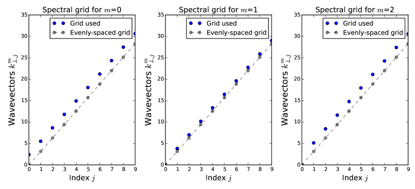
Here, we choose to discretize the algorithm on an evenly-spaced grid in (for the intermediate grid) :
| (17) |
but on an irregular grid in (for the spectral grid). This is because, for the chosen boundary condition (, ), the fields can be expressed as a discrete sum of Bessel modes with
| (18) |
where is the th positive zero of the Bessel function of order (including the trivial value for ; see e.g. [25]). These values are represented in figure 2. Notice that it is not an issue that the spectral components for different azimuthal modes are discretized on different grids, since each azimuthal mode evolves separately in Eqs. 8a, 8b and 8c.
As mentioned above, once this grid is set up, the Discrete Hankel Transform is simply a linear operation on a finite set of points, and can thus be represented by a matrix operation.
| (19) |
Notice that the transformation matrices and depend on (order of the Hankel transform, i.e. order of the Bessel function in the integrand of Eq. 16) and (index of the azimuthal mode, and thus index of the spectral grid on which the Hankel transform is performed). In practice, and are either equal or they differ by (e.g. in Eqs. 14b and 14c, when the azimuthal mode is transformed using the Hankel transform of order or .)
The expressions of and , for the DHT algorithm that we chose, are given in D. In practice, these matrices need to be computed only once (at the beginning of the simulation) and can then be used at each iteration. Notice also that the computational time for this matrix multiplication is proportional to , which is slow compared to a 1D FFT (), but still faster than the 2D FFT () which is typically used in the transverse plane of a spectral 3D Cartesian code.
2.3 Field gathering
In the following, we describe the four successive steps of a PIC cycle with our algorithm in detail, starting with the field gathering. When gathering the fields from the intermediate grid to the macroparticles (see Fig. 1), we use the standard linear shape factors :
| (20) |
where is either or , is either , or , is the index of the macroparticle, and and are the indices of the two nearest cells in and respectively. is the total number of azimuthal modes used, and denotes the real part of a complex quantity. Notice that, in Eq. 20, we used the fact that , which can be inferred from Eq. 12. Incidentally, Eq. 20 shows that only the modes with need to be taken into account in the code, as they are sufficient to retrieve the force on the macroparticles.
Finally, in Eq. 20, and are the linear shape factors in and :
| (21a) | |||
| (21b) |
For particles that are in the lower half of the first radial cell (), Eqs. 20 and 21b require the value although is not actually part of the grid. In order to still apply Eqs. 20 and 21b, we explicitly set , where the sign is chosen whenever the considered field is by definition zero on the axis, and the sign is chosen otherwise. (e.g. is by definition zero on the axis ; see [6] for more details, and for a similar method.)
Note that we use linear shape factors here only for the sake of simplicity, and that higher-order shape factors (e.g. quadratic or cubic) could also be used in principle, with a similar mirroring of the field values across the axis.
2.4 Equations of motion
Since the macroparticles evolve in 3D, we first compute the Cartesian components , , , , and , from the fields , , , , and that were gathered at the positions of each macroparticle. We then advance the equations of motion
| (22) |
in standard 3D Cartesian coordinates by using the leap-frog pusher described in [30].
2.5 Current deposition
As in [6], the charge density is calculated on the intermediate grid in the following way:
| (23) |
where is the charge of the macroparticle with index , and where is the volume of a cell, which is for our grid
| (24) |
Similarly, the current deposition is given by
| (25) |
where and the are the cylindrical components of the velocity of the macroparticle . As mentioned previously, once the macroparticles have deposited their charge and current on the intermediate grid, we transform them to the spectral grid, using an FFT and a DHT (see Fig. 1).
Note that, when a macroparticle travels through the grid, the factor in the above formulas decreases as the macroparticle comes closer to the axis. Therefore, close to the axis, the impact of a single macroparticle on an individual grid cell can be substantial and this generally translates into higher levels of noise. (This is a general problem with cylindrical and quasi-cylindrical codes, and thus it is not specific to the present spectral version.) In order to mitigate this problem, and more generally in order to avoid the accumulation of noise at high frequency, smoothing is typically applied on the charge and currents, after they have been deposited (but no smoothing is applied on the fields and directly). This smoothing is performed directly in spectral space, by multiplying the charge and currents by a transfer function which damps the high frequencies , and whose mathematical form is identical to the spectral Cartesian representation of a single-pass binomial filter [1].
| (26) |
where and are the highest wavevectors that the discrete spectral grid supports, in the longitudinal and transverse direction.
Notice also that, in the above deposition scheme, we do not attempt to reproduce the Esirkepov charge-conserving current deposition [31], and instead use a simple direct current deposition. It is well-known that this simple deposition does not necessarily satisfy the relation , but that this can be corrected, by slightly modifying the currents without modifying their curl (e.g. [32]):
| (27) |
where satisfies the Poisson-like equation
| (28) |
The above equation is typically expensive to solve on a spatial grid, but very easy to solve in spectral space. In spectral space and with the notations of Fig. 1, these equations become
| (29) |
with
| (30) |
With this correction, the new currents do satisfy the charge conservation equation Eq. 10. Therefore we apply this correction in spectral space, at the end of the current deposition at each timestep.
2.6 Integration of the Maxwell equation using the PSATD scheme
The Maxwell equations Eqs. 8a, 8b and 8c could in principle be integrated by using a finite-difference scheme in time, which would be an adaptation of the Cartesian PSTD scheme [13].
| (31a) | ||||
| (31b) | ||||
| (31c) | ||||
| (32a) | ||||
| (32b) | ||||
| (32c) | ||||
| (33a) | ||||
| (33b) | ||||
| (33c) | ||||
However, this type of scheme retains some amount of spurious numerical dispersion, and can thus affect the simulated physics.
Instead, here we use an adaptation of the Cartesian PSATD scheme [10] for our spectral quasi-cylindrical representation. As in the case of the standard PSATD, we assume that the currents are constant over one timestep and that the charge density is linear in time over the same timestep. Under these assumptions, the Maxwell equations Eqs. 8a, 8b and 8c can be integrated analytically over that timestep, and they lead to:
| (34a) | ||||
| (34b) | ||||
| (34c) | ||||
| (35a) | ||||
| (35b) | ||||
| (35c) | ||||
where , and . (See C for a derivation of these equations.)
2.7 Practical implementation
The full PIC algorithm described in this section was implemented in the code FBPIC (Fourier-Bessel Particle-In-Cell), which is written in Python. For performance, this implementation makes use of the pre-compiled libraries FFTW [33] and BLAS [34] (for the matrix multiplication in the DHT), and utilizes the Numba just-in-time compiler [35] for the computationally-intensive parts of the code (current deposition and field gathering). In addition, the code was developed for both single-CPU and single-GPU architectures (with the GPU runs being typically more than 40 times faster than the equivalent CPU runs, on modern hardware). Importantly, a precise timing of the different routines showed that, although the time taken by the spectral transforms (FFT and DHT) is not entirely negligible, it does not usually dominate the PIC cycle. For instance, on a K20 GPU and for a grid with , and 16 particles per cell, the FFTs and DHTs take up 6% and 14% of the PIC cycle respectively, while the rest of the time is dominated by the field gathering and current deposition.
Notice that, even though parallelization is generally challenging for spectral algorithms, a multi-CPU/multi-GPU version could still be developped in the future by using the method of [32]. For the present algorithm, this would involve a domain decomposition along the axis, whereby FFTs would be performed locally within each subdomain and whereby a large number of guard cells would be used in order to mitigate the errors at the border between subdomains. This method based on local FFTs has been studied in the Cartesian context [23], and is now rather well understood. By contrast, performing domain decomposition in the direction would be more challenging, due to the absence of previous work on local Hankel transforms. At any rate, the above considerations for parallel implementation are out of the scope of the present article, and will be the subject of future work. The benchmarks described in the following section use a single-CPU/single-GPU version of the algorithm.
3 Benchmarks
We tested the above algorithm in a number of physical situations. These tests included standard problems, such as e.g. a periodic plasma wave, and involved comparing simulated results to analytical solution, as well as verifying that the algorithm conserves the energy to a satisfying level. For the sake of conciseness, in the present article, we restrict the discussion to the tests of the dispersion relation, since the absence of spurious numerical dispersion was one of the original goals of this algorithm.
3.1 Propagation in vacuum
A first test consisted in letting a laser pulse propagate in vacuum and in measuring its group velocity in the simulation. These simulations were run with the PSATD quasi-cylindrical algorithm presented in Section 2 (see esp. Eqs. 34 and 35), but also, for comparison, with a PSTD version of this same algorithm (see Eqs. 31, 32 and 33), as well as with a finite-difference quasi-cylindrical algorithm equivalent to that of [6, 7] and which had been previously implemented in the PIC code Warp [36].
The simulations were run with a moving window, in a box with a longitudinal size of 40 m and a transverse size of 48 m. (In the case of the spectral algorithm, the fields were damped at the back of the moving window, in a similar way as in [37], in order to prevent periodic wrapping of the fields). The laser pulse itself was initialized at focus, with a waist , a length , a wavelength and a dimensionless potential vector . The resolution was varied while keeping the same cell aspect ratio (). The timestep was set to in the case of the PSATD algorithm, to in the case of the PSTD algorithm, and to in the case of the finite-difference algorithm (for the PSTD and finite-difference algorithms, the chosen is close to the Courant limit).
Physically, the on-axis group velocity of the pulse should be slightly lower than due to the finite waist of the pulse (see e.g. [38]). The analytical expression for the corresponding relative difference in on-axis group velocity is
| (36) |
In the case at hand (, ), this relative difference is extremely small (), and it may be difficult for PIC codes to capture this small physical difference.
To assess the capacities of the finite-difference and spectral codes in this regard, Fig. 3 displays the relative difference in group velocity, as measured in the simulations. As can be observed, in the finite-difference simulations and PSTD simulations, the group velocity of the laser depends on the resolution, due to spurious numerical dispersion. Moreover, in these cases, the group velocity is considerably different than the analytical prediction, even for a relatively high resolution. (Since Fig. 3 does not display the sign of , it is worth noting here that the PSTD algorithm leads to while the finite-difference algorithm has . It is also important to realize here that, although the finite-difference algorithm performs better than the PSTD algorithm in this particular example, this is not generalizable to other cases, as e.g. the numerical dispersion of both algorithms behave differently when or the ratio is changed.)
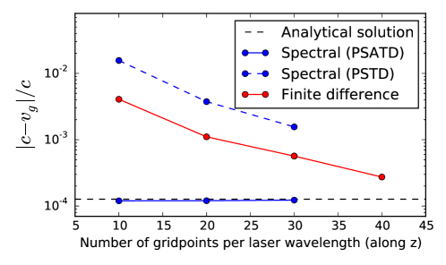
On the other hand, with the PSATD algorithm, the group velocity is practically independent of the resolution, and displays very good agreement with the analytical prediction. This corroborates the fact that the PSATD quasi-cylindrical algorithm described here has no spurious numerical dispersion in vacuum.
Since the PSTD algorithm is less acurate than the PSATD algorithm, while not providing any substantial advantage in terms of speed or practical implementation, we do not consider it further here and perform the rest of the tests with the PSATD algorithm.
3.2 Linear propagation in a plasma
In order to confirm that the spectral algorithm also performs well in the presence of a plasma, we ran the same type of simulations with a uniform, pre-ionized plasma. The numerical parameters of the simulations, as well as the physical parameters of the laser, were the same as in the previous subsection (Section 3.1). The plasma was represented by 16 macroparticles per cell, and had a density , where is the critical density for .
Since the intensity of the laser is very low here (), the propagation is linear, and the on-axis group velocity is given by (e.g. [38])
| (37) |
In Fig. 4, we compare this analytical prediction with the group velocity in the finite-difference and spectral simulations. Again, the group velocity is resolution-dependent in the finite-difference algorithm, and it is substantially different than the analytical prediction even at high resolution. In the spectral code, the group velocity velocity exhibits a very weak dependence on resolution (which is likely due to the errors of current deposition and field gathering on the finite grid). However, its value remains always very close to the analytical prediction at all resolutions.
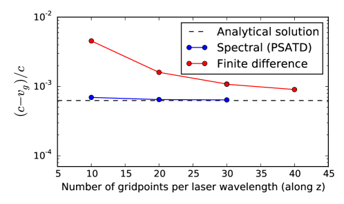
We emphasize that, although the difference between and is small here and may thus seem unimportant, it is this difference which determines the dephasing length and thus the maximum beam energy, in a laser-wakefield simulation. It is therefore paramount to obtain its correct value in the simulation codes. This problem is well-known in the case of standard finite-difference codes. For Cartesian finite-difference codes, a common solution is to use a scheme which is dispersion-free along the axis (e.g. [39, 40, 41]), but no such scheme has been developed for quasi-cylindrical codes. Alternatively, spurious numerical dispersion is often dealt with in finite-difference codes by either using an even finer grid in (which is very computationally expensive) or a coarser grid in . (Recall that, in the simulations shown here, . A coarser resolution in allows to use a slightly larger timestep that approaches , the limit at which spurious numerical dispersion vanishes in the -direction.) However, a coarser resolution in may not always be adapted to resolve the physics of interest, while a finer resolution in is expensive. It is therefore remarkable that, with the spectral quasi-cylindrical algorithm, the correct group velocity is obtained independently of the cell aspect ratio, without having to specifically adapt the resolution in or .
3.3 Linear laser-wakefield
In order to further ascertain that the spectral algorithm described here gives appropriate results beyond simple dispersion tests, we ran a simulation of a laser-wakefield, and compared the amplitude of the wakefield with the corresponding analytical predictions.
In these simulations, the laser was linearly polarized along the transverse direction, and had an amplitude , a wavelength , a length and a waist . The plasma was preionized, with a uniform electron density . As is often the case for simulations of intense laser-plasma interaction (where thermal effects are generally assumed to be negligible), the initial temperature of the plasma is set to 0. The simulation was run in a moving window whose longitudinal and transverse sizes were and . The spatial and temporal resolutions were , and . Since here , the analytical wakefield is given by the linear and quasistatic theory. For a laser of the form – where is the longitudinal envelope of the laser – the longitudinal and transverse fields and are given by (e.g. [8])
| (38a) | |||
| (38b) |
where is the plasma wavevector.
Here, the longitudinal laser envelope was extracted directly from the simulation, and the above analytical integrals where carried out numerically. The resulting predicted fields and are plotted in dashed lines in the left and right lower panels respectively of Fig. 5. These predicted curves are compared with the fields and extracted directly from the simulation (red lines in the lower panels). These fields from the simulation are also displayed as colormaps in the upper panels of Fig. 5, and these colormaps include the line along which the quantities in the lower panels are plotted (dashed line).
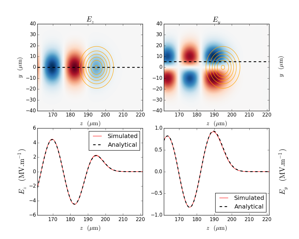
As can be seen on the lower panels of Fig. 5, the analytical and simulated curves overlap very precisely, which confirms the validity of our PIC algorithm. This agreement is all the more remarkable as the field has been extracted from the cells that are closest to the axis, a region where quasi-cylindrical algorithms are typically very noisy.
4 Advantages over finite-difference algorithms
Since finite-difference algorithms and spectral algorithms are considerably different, each of them has its own advantages and shortcomings.
For instance, spectral algorithms – including the one described here – are generally more difficult to parallelize than finite-difference codes. Similarly, the implementation of specific boundary conditions, and of a moving window, is usually more challenging in a spectral algorithm. On the other hand, due to their high accuracy, spectral algorithms can avoid a number of numerical artifacts that are typically present in finite-difference algorithms. This is quite important as, in a finite-difference simulation, these artifacts may remain unnoticed unless additional care is taken in their analysis, and yet they may affect the physics at stake in an important way.
One example of such an artifact is spurious numerical dispersion, which, as mentioned in [4] and in Section 3.2, can modify the dephasing length of a laser-wakefield accelerator – a spurious effect which may be difficult to discern, especially in the cases where there is no analytical formula for this length. As shown in Section 3.2, the algorithm described here would not suffer from this effect, as it is free of spurious numerical dispersion. Similarly, in this section we describe two other typical situations in which our spectral quasi-cylindrical algorithm avoids important artifacts, that would otherwise arise in a finite-difference code.
4.1 Suppression of zero-order numerical Cherenkov effect
A first artifact which is avoided is the zero-order numerical Cherenkov effect. To zero order, the numerical Cherenkov effect is a consequence of the spurious numerical dispersion [3], and arises because some relativistic particles can travel faster than the numerically-altered velocity of the electromagnetic waves, in the simulations. This typically causes these relativistic particles to emit a characteristic spurious radiation. Recently, it was shown that this spurious radiation can have a very substantial impact in lab-frame simulations of laser-wakefield acceleration, in particular by spuriously increasing the emittance of the accelerated beam [42]. It was also shown that, by modifying the PIC algorithm and its numerical dispersion relation, the zero-order Cherenkov radiation can be suppressed. (Notice that there exists also a set of higher-order, aliased numerical Cherenkov effects, which are not as easily suppressed [43, 44, 14, 15, 16, 17, 45]. These high-order effects can lead to disruptive instabilities in boosted-frame simulations, but on the other hand no such instability was observed in typical lab-frame simulations of laser-plasma acceleration. It is in fact likely that these instabilities may not have enough time to develop in the case of typical lab-frame simulations.)
Since the spectral quasi-cylindrical algorithm described here is dispersion-free, it should not exhibit the zero-order numerical Cherenkov effect. In order to confirm this prediction, we ran a simulation of laser-wakefield acceleration with our spectral quasi-cylindrical algorithm, and compared it with an equivalent simulation that uses the finite-difference quasi-cylindrical algorithm of Warp.
In these simulations, a laser pulse with a waist , a length , an amplitude and a wavelength is sent into a longitudinally-shaped pre-ionized gas jet. The gas jet has a 100 -long rising density gradient at its entrance, followed by a 200 plateau at a density and then by a 100 -long downramp, so as to finally reach a density . Again, the initial temperature of the plasma is set to 0. The downramp causes the injection of an electron beam, which is then accelerated in the subsequent density plateau at . Both the spectral and the finite-difference simulations were run in a moving window whose longitudinal and transverse dimensions were 160 and 48 , and both simulations used a resolution and . Again, the finite-difference simulation was run with a timestep while the spectral simulation was run with . Importantly, the charge and currents are smoothed in both simulations. The spectral algorithms performs smoothing in spectral space as described in Section 2.5, while the finite-difference algorithm applies a single-pass binomial filter on the spatial grid, in both the and directions.
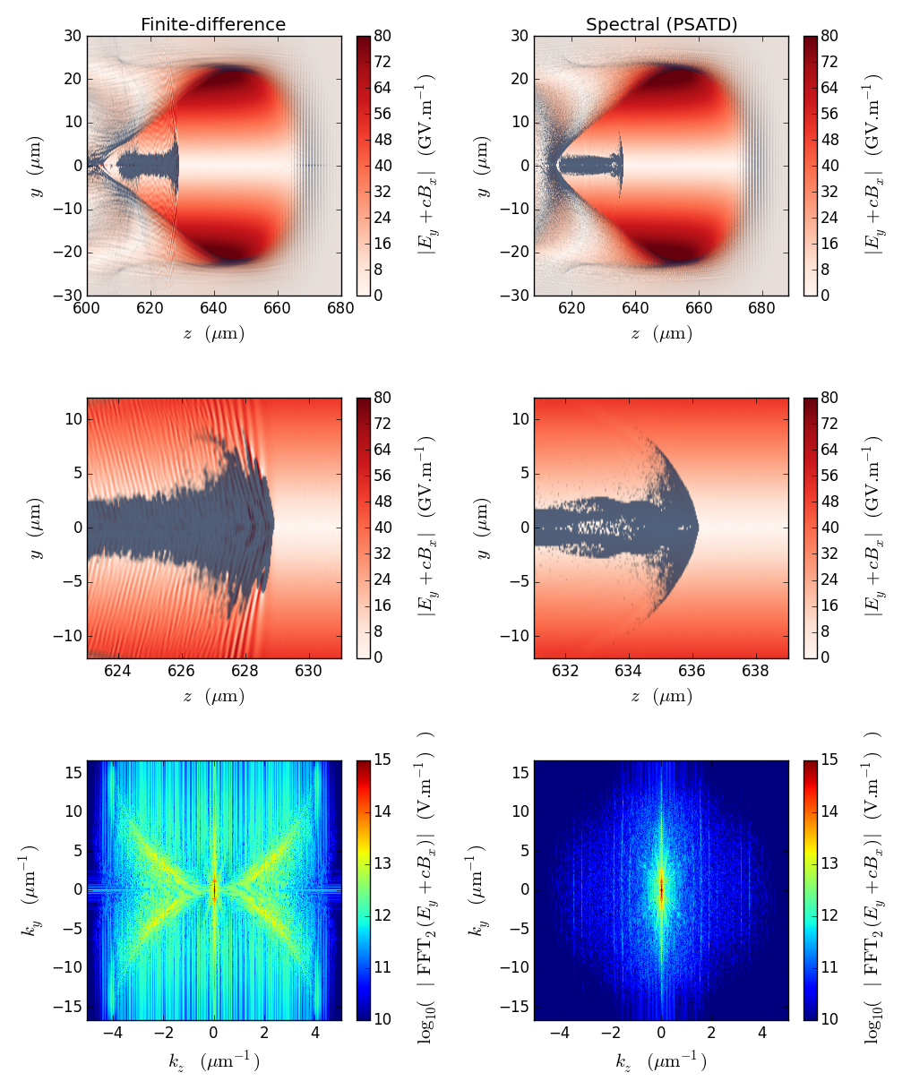
Figure 6 shows a snapshot of the two simulations, at a similar physical time. The red colormap represents the quantity , while the superimposed shades of blue represent the electron density. (The quantity is chosen because it corresponds to the component of the Lorentz force felt by a relativistic electron having .) As can be seen in the top panels, the global aspect of the bubble and of the injected bunch is similar in both simulations. In particular, the injected charge was found to be almost the same (766 pC with the finite-difference algorithm and 750 pC with the spectral algorithm). However, a closer look at the bunch in the finite-difference algorithm (see the middle left panel in Fig. 6) reveals that the bunch emits a high-frequency radiation. This radiation seems to be due to the zero-order numerical Cherenkov effect – an interpretation which is confirmed by the observation of the corresponding characteristic double-parabola in space [42, 43, 44] on the lower left panel of Fig. 6. Importantly, the amplitude of this unphysical field, in the middle panel of Fig. 6, happens to be comparable to the focusing fields inside the bubble, and it can thus potentially affect the bunch in a substantial manner. On the other hand, the spectral algorithm does not exhibit this unphysical radiation in real space (see the middle right panel in Fig. 6), nor does it exhibit the corresponding characteristic pattern in space (see the lower right panel). This was indeed expected from its dispersion-free property, and it confirms the fact that our spectral quasi-cylindrical algorithm is free of the unphysical artifacts associated with the zero-order numerical numerical Cherenkov effect.
For completeness, we remark that a similar suppression of the numerical Cherenkov radiation was obtained in [42, 4], by using modified finite-difference algorithms. However, it is important to note that these algorithms were applicable to a Cartesian PIC code, but not to a quasi-cylindrical code. An adaptation to cylindrical geometry is proposed in [46], and was shown to efficiently suppress zero-order numerical Cherenkov effect. However, this adaptation is not, strictly speaking, dispersion-free.
4.2 Accurate force of a laser on a copropagating electron
Another case in which our spectral algorithm performs better than finite-difference algorithms is whenever a relativistic electron bunch overlaps with a copropagating laser. This situation occurs for instance in laser-wakefield acceleration, when the accelerated electron bunch progressively catches up with the laser pulse and may eventually overlap with it (e.g. [47, 48]). It is also the typical configuration for simulations of free-electron lasers, where the overlap of the electron bunch and the copropagating laser radiation, inside an undulator, leads to a growing instability.
Despite the practical importance of this physical configuration, it was recently shown that standard finite-difference PIC codes tend to largely overestimate the force felt by the electrons inside a copropagating laser (see the appendix of [49]). This overestimation was shown to be mainly due to the staggering in time of the and fields in a standard finite-difference code. This staggering indeed results in an improper numerical compensation of the two terms of the Lorentz force . However, in our spectral quasi-cylindrical algorithm, the fields and are not staggered in time, and thus the force on a copropagating electron bunch should be correct.
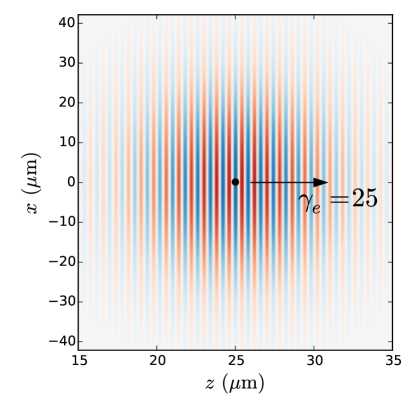
To confirm this prediction, we ran a test simulation in which a single relativistic macroparticle copropagates with a laser pulse. The initial configuration of the simulation is represented in Fig. 7. The laser pulse is polarized along and is characterized by a waist , a length , an amplitude and a wavelength , while the macroparticle represents a relativistic electron having an initial Lorentz factor . For comparison, the simulation was run, again, with both our spectral quasi-cylindrical algorithm and the finite-difference quasi-cylindrical algorithm of Warp. In order to study numerical convergence, the simulations were run with various longitudinal resolution , but with a fixed cell aspect ratio . The timestep was again for the finite-difference simulation and for the spectral simulation. Finally, the simulations were run in a moving window with a longitudinal and transverse size of 40 and 60 respectively.
In order to assess the correctness of the force felt by the electron, we analyze the evolution of its transverse momentum in time. Analytically, it can be shown from the Lagrangian that the equation of motion along the axis (i.e. the axis of laser polarization) is
| (39) |
where is the normalized vector potential of the laser pulse. The right-hand side corresponds to the ponderomotive force, and, for the parameters and timescale considered here, it is in fact negligible. The canonical momentum of the electron is thus approximately conserved.
| (40) |
Since, inside the laser pulse, oscillates between the values and , the quantity is predicted to also also oscillate between and , as the electron progressively dephases with the laser.
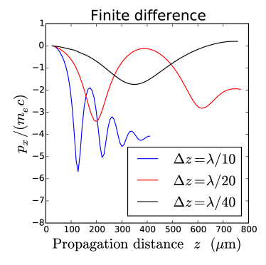
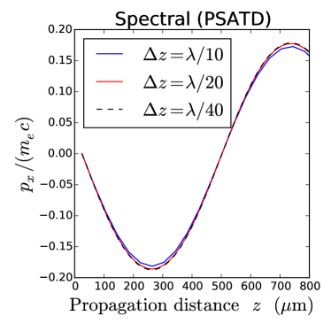
Keeping in mind that here initially , one can observe on Fig. 8 that the oscillation amplitude of is much higher than analytically predicted in the finite-difference simulation. In addition, these oscillations strongly depend on the resolution of the simulation, which confirms their spurious nature. These observations are consistent with those of [49], and they are due to the above-mentioned erroneous calculation of the Lorentz force. On the other hand, in the spectral simulations, the oscillations of exhibits virtually no dependence on the resolution. In addition, the oscillations of have a realistic amplitude. (The fact that these oscillations do not reach exactly the value 0.2 may be due to the fact that decreases as the laser propagates, as a consequence of diffraction.) These observations confirm that the spectral quasi-cylindrical algorithm properly calculates the Lorentz force on the electron. This is also consistent with our expectations, which were based on the fact that and fields are not staggered in time, in this algorithm.
Conclusion
In this article, we derived the equations of a spectral quasi-cylindrical PIC algorithm, and discussed its numerical implementation. As explained in the text, because this algorithm is quasi-cylindrical, it requires much less computational time and memory than a full 3D algorithm. In addition, the fact that it is spectral (and uses the PSATD algorithm) prevents a certain number of artifacts, that are usually present in a finite-difference algorithm.
This second aspect was tested in detail in this article, through several benchmarks. By comparing simulations with analytical results, we showed that our spectral quasi-cylindrical code is free of spurious numerical dispersion, that it does not exhibit zero-order numerical Cherenkov effect in typical lab-frame simulations, and that it can accurately calculate the force of a laser on a copropagating electron. By running the same benchmarks with a finite-difference quasi-cylindrical algorithm, we showed that these numerical artifacts can, on the contrary, be present in finite-difference PIC algorithms.
However, it must not be forgotten that finite-difference algorithms have advantages of their own, including easier parallelization and application of boundary conditions. In the case of our spectral quasi-cylindrical algorithm, parallelization to several nodes could nonetheless be achieved by following for instance the method of [32]. This will be the subject of future work.
Acknowledgements
We thank Axel Huebl of the PIConGPU team [50] for interesting discussions on the GPU implementation, and Kevin Peters (U. Hamburg) for contributing to the validation of the code. We acknowledge computational resources from the Physnet cluster, University of Hamburg.
This work was supported by the Director, Office of Science, Office of High Energy Physics, U.S. Dept. of Energy under Contract No. DE-AC02-05CH11231, including from the Laboratory Directed Research and Development (LDRD) funding from Berkeley Lab.
This document was prepared as an account of work sponsored in part by the United States Government. While this document is believed to contain correct information, neither the United States Government nor any agency thereof, nor The Regents of the University of California, nor any of their employees, nor the authors makes any warranty, express or implied, or assumes any legal responsibility for the accuracy, completeness, or usefulness of any information, apparatus, product, or process disclosed, or represents that its use would not infringe privately owned rights. Reference herein to any specific commercial product, process, or service by its trade name, trademark, manufacturer, or otherwise, does not necessarily constitute or imply its endorsement, recommendation, or favoring by the United States Government or any agency thereof, or The Regents of the University of California. The views and opinions of authors expressed herein do not necessarily state or reflect those of the United States Government or any agency thereof or The Regents of the University of California.
Appendix A Derivation of the spectral quasi-cylindrical representation
In order to derive the representation Eqs. 6a, 6b and 6c, we have to distinguish the Cartesian components (e.g. , , , , , ), which are well-defined everywhere in space and thus have a regular Fourier representation, from the cylindrical components (e.g. , , , ), which are ill-defined at . (For instance, for a field of the form , the expression of is , which ill-defined at , as itself is ill-defined at this position.)
A.1 Cartesian components
Let be the Cartesian component of a field (typically is , or and is , or ). Its Fourier representation is thus given by Eqs. 2 and 3:
| (41) | |||
| (42) |
Using the change of variable , , , , this becomes
| (43) | |||
| (44) |
Let us now use the relation (which is simply another way of writing the well-known relation ). The above equations become:
| (45) | |||
| (46) |
We now define . This results in the following equations :
| (47) | |||
| (48) |
A.2 Cylindrical components
Let us now consider fields of the type , or , which we denote generally by . We have :
| (49) |
Using Eq. 48 leads to
| (50) |
| (51) |
where we relabeled the dummy variable in the above sums. Let us thus define and . This results in:
| (52) |
With the same definitions and the same method, it is also easy to show that:
| (53) |
Appendix B Maxwell equations for the spectral coefficients
In this section, let us derive the Maxwell equations for the spectral coefficients Eqs. 8a, 8b and 8c from the Maxwell equations written in cylindrical coordinates Eqs. 5a, 5b and 5c.
When replacing the Fourier-Hankel decomposition (Eqs. 48, 6b and 6c) in the Maxwell equations Eqs. 5a, 5b and 5c, we first notice that the modes proportional to for different values of and are not coupled. These different modes can thus be treated separately. The same cannot be said of the modes corresponding to different values of , since they may be coupled through the Bessel functions and their derivatives. In the following, we write only the equations corresponding to , since the equation can be treated very similarly. These equations become
| (54a) | ||||
| (54b) | ||||
| (54c) | ||||
By taking the sum and difference of the first two equations, and by rearranging the third equation, we obtain:
| (55a) | |||
| (55b) | |||
| (55c) | |||
We can now use the relations and (see relation 9.1.27 in [51]), and obtain :
| (56a) | |||
| (56b) | |||
| (56c) | |||
Each equation of the above system contains Bessel functions of only one given order (, or ). This allows the different components to be separated, since the functions , for a fixed and different values of , form a basis of the set of real functions:
| (57a) | |||
| (57b) | |||
| (57c) | |||
Appendix C PSATD scheme, in the Fourier-Hankel representation
We use a scheme very similar to that of [10]. In this scheme the currents are considered constant over one timestep, and the charge density is considered linear in time.
C.1 Expressions for
By combining Eqs. 8a, 8b and 8c and Eq. 9, one can find the propagation equations for .
| (58a) | |||
| (58b) | |||
| (58c) | |||
Let us integrate these equations for . In this interval, is constant and equal to , and thus the right-hand side of the above equations is constant. Using Green functions, the general solution of a differential equation of the form , where is a constant, is
| (59) |
We thus use the above expression, with , to integrate the fields from to . In particular, we use again the Maxwell equations Eqs. 8a, 8b and 8c to obtain the expression of . This yields:
| (60a) | ||||
| (60b) | ||||
| (60c) | ||||
where and .
C.2 Expressions for
Similarly, when combining Eqs. 8a, 8b and 8c and Eq. 9, the propagation equations for are:
| (61a) | |||
| (61b) | |||
| (61c) | |||
Let us again integrate these equations for . In this interval, is constant (thus its time derivatives drop), and is linear in time. As a consequence the right hand side is proportional to . Using Green functions, the solution of is
| (62) |
which, for , reduces to
| (63) |
Using the above expression, we obtain
| (64a) | ||||
| (64b) | ||||
| (64c) | ||||
Appendix D Discrete Hankel Transform
D.1 Calculation of the transformation matrices and
Here, for the Discrete Hankel Transform, we use a transformation similar to that of [27, 25, 29], but we extend it to the case of an evenly-spaced grid in real space (as opposed to one that is distributed according to the zeros of the Bessel function, which would have been inconvenient for current deposition and field gathering). Moreover, we impose, as much as possible, that the succession of a Discrete Hankel Transform (DHT) and an Inverse Discrete Hankel Transform (IDHT) retrieves the initial function. As explained in the text of the article, we use a matrix formalism for the DHT:
| (65) |
where is the order of the Hankel transform, and where is the index of the spectral grid on which the Hankel transform is evaluated. In practice, as mentioned in the text, these transforms are only used in the cases , or .
The matrices and can be entirely determined by a set of constraints. These constraints can be found, for instance, by imposing the value of the DHT for a set of different functions, whose exact analytical Hankel transforms are known. In our case, we impose that the DHT be equal to the exact analytical Hankel transform for the eigenmodes of a cavity with perfectly conducting boundary at (), since these physical eigenmodes should also be eigenmodes of our PIC cycle. These eigenmodes have the following form:
| (66a) | ||||
| (66b) | ||||
| (66c) | ||||
where is the Heaviside function and where , with the th positive zero of the Bessel function of order . The exact Hankel transform of these modes, evaluated on the discrete set reads (see D.2 for a derivation)
| (67) |
where is either , or . Note that the above relation is valid for any value of , , and (provided that ), except when , and simultaneously (again, see D.2 for an explanation). Here we impose that the DHT is consistent with Eq. 67, where applicable
| (68) |
and we use the constraints given by Eq. 68 to obtain the matrix .
Case where or
In this case, Eq. 68 is applicable for any and in , and thus this provides constraints on the matrix , which allow one to completely determine it. In fact, a closer look at Eq. 68 shows that the inverse matrix can be directly extracted from the above relations, since this inverse matrices is defined by the relation . Thus, from the above relations, one can directly infer:
| (69) |
The matrix can then be extracted, by numerically inverting the matrices given by the above expression. In addition, we impose that be exactly equal to , so that the succession of a DHT and IDHT retrieves exactly the initial function.
Case where and
In this case, the equation Eq. 68 is not valid for , and thus it provides only constraints on the matrix , which is not enough to completely determine it. In this case, we use an empirical method in which we impose the additional constraints
| (70) |
This constraint is imposed because we choose the amplitude of the Hankel mode proportional to to be 0 in the simulation. (For and , for any , so that the amplitude of the corresponding mode has no physical meaning whatsoever.) This allows the matrix to be entirely determined. In addition, to obtain , we impose for any (as in the case or ), but also for . This is done again for consistency with the fact that . We note that the above method gives satisfying results for but not for . In the future, further work will be done towards a better Hankel transform representation.
D.2 Derivation of Eq. 67
Let us first remark that, through a change of variable where , Eq. 67 is equivalent to
| (71) |
and let us prove this equation for different cases, excluding the case where , and and in which it is not valid.
Case where and
In this case, we use the relation 11.4.5 of [51]. Since , and since by definition is the zero of the Bessel function of order , we have , and the relation 11.4.5 is thus used in the case and (see relation 11.4.5 in [51] for the definition of the and coefficients). This yields
| (72) |
where we further used the relation 9.1.27 in [51], which reads , and took into account the fact that in our case.
Case where and
Case where and
The proof of the two above cases used the relation 11.4.5 from [51], which is applicable as long as . This is the case for (i.e. the two above cases) but also for and (i.e. and thus ). As a consequence, the above proofs are also valid for and .
Case where , and
References
-
[1]
C. Birdsall, A. Langdon,
Plasma Physics via
Computer Simulation, Series in Plasma Physics, Taylor & Francis, 2004.
URL http://books.google.fr/books?id=S2lqgDTm6a4C -
[2]
R. Hockney, J. Eastwood,
Computer Simulation Using
Particles, Taylor & Francis, 1988.
URL http://books.google.fr/books?id=nTOFkmnCQuIC -
[3]
B. B. Godfrey, Journal of Computational Physics 15 (4) (1974) 504 – 521.
doi:10.1016/0021-9991(74)90076-X,
[link].
URL http://www.sciencedirect.com/science/article/pii/002199917490076X -
[4]
B. M. Cowan, D. L. Bruhwiler, J. R. Cary, E. Cormier-Michel, C. G. R. Geddes,
Phys. Rev. ST Accel. Beams 16 (2013) 041303.
doi:10.1103/PhysRevSTAB.16.041303,
[link].
URL http://link.aps.org/doi/10.1103/PhysRevSTAB.16.041303 -
[5]
B. Godfrey, The IPROP
Three-Dimensional Beam Propagation Code, Defense Technical Information
Center, 1985.
URL https://books.google.com/books?id=hos_OAAACAAJ -
[6]
A. F. Lifschitz, X. Davoine, E. Lefebvre, J. Faure, C. Rechatin, V. Malka, J.
Comput. Phys. 228 (5) (2009) 1803–1814.
doi:10.1016/j.jcp.2008.11.017,
[link].
URL http://dx.doi.org/10.1016/j.jcp.2008.11.017 - [7] A. Davidson, A. Tableman, W. An, F. S. Tsung, W. Lu, J. Vieira, R. A. Fonseca, L. O. Silva, W. B. Mori, Journal of Computational Physics 281 (2015) 1063–1077. arXiv:1403.6890, doi:10.1016/j.jcp.2014.10.064.
-
[8]
E. Esarey, C. B. Schroeder, W. P. Leemans, Rev. Mod. Phys. 81 (2009)
1229–1285.
doi:10.1103/RevModPhys.81.1229,
[link].
URL http://link.aps.org/doi/10.1103/RevModPhys.81.1229 -
[9]
A. T. Lin, J. M. Dawson, H. Okuda, Physics of Fluids 17 (11) (1974) 1995–2001.
doi:http://dx.doi.org/10.1063/1.1694656,
[link].
URL http://scitation.aip.org/content/aip/journal/pof1/17/11/10.1063/1.1694656 - [10] I. Haber, R. Lee, H. Klein, J. Boris, 1973.
-
[11]
O. Buneman, C. Barnes, J. Green, D. Nielsen,
Principles
and capabilities of 3-d, e-m particle simulations, Journal of Computational
Physics 38 (1) (1980) 1 – 44.
doi:http://dx.doi.org/10.1016/0021-9991(80)90010-8.
URL http://www.sciencedirect.com/science/article/pii/0021999180900108 -
[12]
J. M. Dawson, Rev. Mod. Phys. 55 (1983) 403–447.
doi:10.1103/RevModPhys.55.403,
[link].
URL http://link.aps.org/doi/10.1103/RevModPhys.55.403 -
[13]
Q. H. Liu, Microwave and Optical Technology Letters 15 (3) (1997) 158–165.
doi:10.1002/(SICI)1098-2760(19970620)15:3<158::AID-MOP11>3.0.CO;2-3,
[link].
URL http://dx.doi.org/10.1002/(SICI)1098-2760(19970620)15:3<158::AID-MOP11>3 %****␣Spectral_circ.bbl␣Line␣100␣****.0.CO;2-3 -
[14]
B. B. Godfrey, J.-L. Vay, I. Haber, Journal of Computational Physics 258 (2014)
689 – 704.
doi:http://dx.doi.org/10.1016/j.jcp.2013.10.053,
[link].
URL http://www.sciencedirect.com/science/article/pii/S0021999113007298 - [15] B. Godfrey, J.-L. Vay, I. Haber, Plasma Science, IEEE Transactions on 42 (5) (2014) 1339–1344. doi:10.1109/TPS.2014.2310654.
-
[16]
P. Yu, X. Xu, V. K. Decyk, W. An, J. Vieira, F. S. Tsung, R. A. Fonseca, W. Lu,
L. O. Silva, W. B. Mori, Journal of Computational Physics 266 (2014) 124 –
138.
doi:http://dx.doi.org/10.1016/j.jcp.2014.02.016,
[link].
URL http://www.sciencedirect.com/science/article/pii/S0021999114001363 -
[17]
P. Yu, X. Xu, V. K. Decyk, F. Fiuza, J. Vieira, F. S. Tsung, R. A. Fonseca,
W. Lu, L. O. Silva, W. B. Mori, Computer Physics Communications 192 (2015) 32
– 47.
doi:http://dx.doi.org/10.1016/j.cpc.2015.02.018,
[link].
URL http://www.sciencedirect.com/science/article/pii/S0010465515000752 -
[18]
J.-L. Vay, Phys. Rev. Lett. 98 (2007) 130405.
doi:10.1103/PhysRevLett.98.130405,
[link].
URL http://link.aps.org/doi/10.1103/PhysRevLett.98.130405 -
[19]
S. F. Martins, R. A. Fonseca, W. Lu, W. B. Mori, L. O. Silva, Nat Phys 6 (4)
(2010) 311–316.
[link].
URL http://dx.doi.org/10.1038/nphys1538 -
[20]
J.-L. Vay, C. Geddes, E. Cormier-Michel, D. Grote, Journal of Computational
Physics 230 (15) (2011) 5908 – 5929.
doi:http://dx.doi.org/10.1016/j.jcp.2011.04.003,
[link].
URL http://www.sciencedirect.com/science/article/pii/S0021999111002270 -
[21]
P. Yu, X. Xu, A. Tableman, V. K. Decyk, F. S. Tsung, F. Fiuza,
A. Davidson, J. Vieira, R. A. Fonseca, W. Lu, L. O. Silva, W. B.
Mori, ArXiv e-printsarXiv:1502.01376, [link].
URL http://arxiv.org/abs/1502.01376 -
[22]
I. Andriyash, R. Lehe, V. Malka, Journal of Computational Physics 282 (2015)
397 – 409.
doi:http://dx.doi.org/10.1016/j.jcp.2014.11.026,
[link].
URL http://www.sciencedirect.com/science/article/pii/S0021999114007888 - [23] H. Vincenti, J. Vay, ArXiv e-printsarXiv:1507.05572.
-
[24]
P. Lee, J.-L. Vay, Computer Physics Communications 194 (2015) 1 – 9.
doi:http://dx.doi.org/10.1016/j.cpc.2015.04.004,
[link].
URL http://www.sciencedirect.com/science/article/pii/S0010465515001356 -
[25]
M. Guizar-Sicairos, J. C. Gutiérrez-Vega, J. Opt. Soc. Am. A 21 (1) (2004)
53–58.
doi:10.1364/JOSAA.21.000053,
[link].
URL http://josaa.osa.org/abstract.cfm?URI=josaa-21-1-53 -
[26]
M. Cree, P. Bones, Computers & Mathematics with Applications 26 (1) (1993) 1
– 12.
doi:http://dx.doi.org/10.1016/0898-1221(93)90081-6,
[link].
URL http://www.sciencedirect.com/science/article/pii/0898122193900816 -
[27]
L. Yu, M. Huang, M. Chen, W. Chen, W. Huang, Z. Zhu, Opt. Lett. 23 (6) (1998)
409–411.
doi:10.1364/OL.23.000409,
[link].
URL http://ol.osa.org/abstract.cfm?URI=ol-23-6-409 -
[28]
A. E. Siegman, Opt. Lett. 1 (1) (1977) 13–15.
doi:10.1364/OL.1.000013,
[link].
URL http://ol.osa.org/abstract.cfm?URI=ol-1-1-13 -
[29]
Y. Kai-Ming, W. Shuang-Chun, C. Lie-Zun, W. You-Wen, H. Yong-Hua, Chinese
Physics B 18 (9) (2009) 3893.
[link].
URL http://stacks.iop.org/1674-1056/18/i=9/a=046 -
[30]
J.-L. Vay, Physics of Plasmas (1994-present) 15 (5) (2008) 056701.
doi:http://dx.doi.org/10.1063/1.2837054,
[link].
URL http://scitation.aip.org/content/aip/journal/pop/15/5/10.1063/1.2837054 -
[31]
T. Esirkepov, Computer Physics Communications 135 (2) (2001) 144 – 153.
doi:http://dx.doi.org/10.1016/S0010-4655(00)00228-9,
[link].
URL http://www.sciencedirect.com/science/article/pii/S0010465500002289 -
[32]
J.-L. Vay, I. Haber, B. B. Godfrey, Journal of Computational Physics 243 (2013)
260 – 268.
doi:http://dx.doi.org/10.1016/j.jcp.2013.03.010,
[link].
URL http://www.sciencedirect.com/science/article/pii/S0021999113001873 -
[33]
Fftw.
URL http://www.fftw.org/ -
[34]
Blas.
URL http://www.netlib.org/blas/ -
[35]
Numba.
URL http://numba.pydata.org/ -
[36]
J.-L. Vay, D. P. Grote, R. H. Cohen, A. Friedman, Computational Science &
Discovery 5 (1) (2012) 014019.
[link].
URL http://stacks.iop.org/1749-4699/5/i=1/a=014019 - [37] P. Yu, A. Davidson, A. Tableman, V. K. Decyk, F. S. Tsung, W. B. Mori, 2015.
-
[38]
E. Esarey, W. P. Leemans, Phys. Rev. E 59 (1999) 1082–1095.
doi:10.1103/PhysRevE.59.1082,
[link].
URL http://link.aps.org/doi/10.1103/PhysRevE.59.1082 - [39] M. Karkkainen, E. Gjonaj, T. Lau, T. Weiland, Vol. 1, Chamonix, France, 2006.
- [40] A. Pukhov, Journal of Plasma Physics 61 (03) (1999) 425–433. doi:null.
-
[41]
R. Nuter, M. Grech, P. Gonzalez de Alaiza Martinez, G. Bonnaud,
E. d’Humières, The European Physical Journal D 68 (6).
doi:10.1140/epjd/e2014-50162-y,
[link].
URL http://dx.doi.org/10.1140/epjd/e2014-50162-y -
[42]
R. Lehe, A. Lifschitz, C. Thaury, V. Malka, X. Davoine, Phys. Rev. ST Accel.
Beams 16 (2013) 021301.
doi:10.1103/PhysRevSTAB.16.021301,
[link].
URL http://link.aps.org/doi/10.1103/PhysRevSTAB.16.021301 -
[43]
B. B. Godfrey, J.-L. Vay, Journal of Computational Physics 248 (2013) 33 – 46.
doi:http://dx.doi.org/10.1016/j.jcp.2013.04.006,
[link].
URL http://www.sciencedirect.com/science/article/pii/S0021999113002556 -
[44]
X. Xu, P. Yu, S. F. Martins, F. S. Tsung, V. K. Decyk, J. Vieira, R. A.
Fonseca, W. Lu, L. O. Silva, W. B. Mori, Computer Physics Communications
184 (11) (2013) 2503 – 2514.
doi:http://dx.doi.org/10.1016/j.cpc.2013.07.003,
[link].
URL http://www.sciencedirect.com/science/article/pii/S0010465513002312 -
[45]
B. B. Godfrey, J.-L. Vay, Computer Physics Communications (2015) –doi:http://dx.doi.org/10.1016/j.cpc.2015.06.008,
[link].
URL http://www.sciencedirect.com/science/article/pii/S0010465515002532 -
[46]
R. Lehe, Theses, Ecole Polytechnique (Jul. 2014).
[link].
URL https://pastel.archives-ouvertes.fr/tel-01088398 -
[47]
S. Cipiccia, M. R. Islam, B. Ersfeld, R. P. Shanks, E. Brunetti, G. Vieux,
X. Yang, R. C. Issac, S. M. Wiggins, G. H. Welsh, M.-P. Anania, D. Maneuski,
R. Montgomery, G. Smith, M. Hoek, D. J. Hamilton, N. R. C. Lemos, D. Symes,
P. P. Rajeev, V. O. Shea, J. M. Dias, D. A. Jaroszynski, Nat Phys 7 (11)
(2011) 867–871.
[link].
URL http://dx.doi.org/10.1038/nphys2090 -
[48]
K. Németh, B. Shen, Y. Li, H. Shang, R. Crowell, K. C. Harkay, J. R. Cary,
Phys. Rev. Lett. 100 (2008) 095002.
doi:10.1103/PhysRevLett.100.095002,
[link].
URL http://link.aps.org/doi/10.1103/PhysRevLett.100.095002 -
[49]
R. Lehe, C. Thaury, E. Guillaume, A. Lifschitz, V. Malka, Phys. Rev. ST Accel.
Beams 17 (2014) 121301.
doi:10.1103/PhysRevSTAB.17.121301,
[link].
URL http://link.aps.org/doi/10.1103/PhysRevSTAB.17.121301 -
[50]
M. Bussmann, H. Burau, T. E. Cowan, A. Debus, A. Huebl, G. Juckeland, T. Kluge,
W. E. Nagel, R. Pausch, F. Schmitt, U. Schramm, J. Schuchart, R. Widera, in:
Proceedings of the International Conference on High Performance Computing,
Networking, Storage and Analysis, SC ’13, ACM, New York, NY, USA, 2013, pp.
5:1–5:12.
doi:10.1145/2503210.2504564,
[link].
URL http://doi.acm.org/10.1145/2503210.2504564 - [51] M. Abramowitz, I. Stegun, Handbook of Mathematical Functions, Dover Publications, 1972.