Halo Profile Evolution and Velocity Bias

Abstract

We propose a simple model that elucidates the generation of halo velocity bias. The fluid equation approximation is often adopted in modelling the evolution of the halo density field. In this approach, halos are often taken to be point particles even though in reality they are finite-sized objects. In this paper, we generalize the fluid equation approximation to halos to include the finite extent of halos by taking into account the halo profile. We compute the perturbation of the halo density and velocity field to second order and find that the profile correction gives rise to $k^{2}$ correction terms in Fourier space. These corrections are more important for velocity than for density. In particular, the profile correction generates $k^{2}$ correction term in the velocity bias and the correction terms do not decay away in the long term limit, but it is not constant. We model the halo profile evolution using the spherical collapse model. We also measure the evolution of proto-halo profile at various redshifts numerically. We find that the spherical collapse model gives a reasonable description of the numerical profile evolution. Static halo profile is often adopted in modelling halos in theories such as the excursion set theory. Our work highlights the importance of including the profile evolution in the calculations.

I Introduction

Peculiar velocity can be a powerful probe of cosmology. On one hand, peculiar velocity causes redshift space distortion Kaiser (1987), thus to get cosmological information from galaxy surveys, one needs to model the peculiar velocity as well. On the other hand, redshift space distortion causes anisotropy, which gives rise to higher order multipoles in the correlation function/power spectrum Hamilton (1992), and hence a useful signal. Peculiar velocity can also help distinguish general relativity from modified gravity, e.g. Song and Percival (2009); Taruya et al. (2014). The redshift space distortion has been used to constrain the growth rate and testing gravity from some recent galaxy surveys Guzzo et al. (2008); Blake et al. (201); Reid et al. (2012); Beutler et al. (2012); Samushia et al. (2013); de la Torre et al. (2013); Oka et al. (2014). In future the peculiar velocity surveys can also be fruitful Koda et al. (2014).

As in galaxy surveys, only galaxies are observable, not the dark matter, it is important to understand if the velocity of the galaxy is biased with respect to that of the underlying dark matter or not. As galaxies are hosted in halos, and halos are simpler than galaxies because they are only governed by the gravitational physics, in this paper, we take studying the halo bias as a step towards understanding the galaxy bias. Recently there have been some indications from the measurements using halos at low redshifts that velocity bias may be non-negligible, although the quantitative measurement is still hard Elia et al. (2002); Chan et al. (2012); Baldauf et al. (2014); Jennings et al. (2014); Zheng et al. (2014a). Velocity measurement is nontrivial because it requires the velocity field of the tracers to be weighted by volume, and it is easy to mistakenly get the density weighted velocity, i.e. momentum, instead of velocity Scoccimarro (2004). When the number density of the tracers is low, it suffers from numerical sampling artifact, see e.g. Juszkiewicz et al. (1995); Zhang et al. (2014); Zheng et al. (2014b, a). One way out is to use momentum instead, e.g. in Okumura et al. (2012); Baldauf et al. (2014). Unlike the velocity field, however, there is an additional complication that in momentum the galaxy density bias is involved as well.

On the theory side, in the usual fluid approximation for dark matter and galaxy, even if the initial velocity field of the galaxy differs from that of the dark matter, i.e. there is initial velocity bias, large scale gravitational evolution will naturally drive the galaxy velocity field to that of the dark matter Elia et al. (2011); Chan et al. (2012). On the other hand, the peak model predicts that the velocity bias persists and remains constant at late time Desjacques et al. (2010). This result seems to be favoured by the recent simulation results, which suggest that the halo velocity bias at late time is non-negligible at $k\sim 0.15\,\mathrm{Mpc}^{-1}\,h$. Ref. Baldauf et al. (2014) argued that the force on the halo has to be “biased” in order for the coupled-fluid approach to agree with peak model result, although no further justification was given. Ref. Biagetti et al. (2014a) tried to derive the peak theory results using the distribution function approach. Here we take a different approach. A halo is a composite object consisting of a collection of particles. The position of the halo is defined by the position of the center of mass (CM) of its constituent particles. Thus the force acting on the CM position of the halo should be averaged over its constituent particles. In this way, we give a physical origin for the “biased” force on the halo. We will show that the halo profile correction naturally gives rise to the leading $k^{2}$ correction to the velocity bias and it does not decay away.

We note that our approach also has rather different interpretation for the generation of velocity bias from that in Desjacques and Sheth (2010); Desjacques et al. (2010); Baldauf et al. (2014); Biagetti et al. (2014a). In peak theory, although the smoothing window is an important ingredient, the window function is usually assumed to be static. Sometimes, the attention is focused on the discrete peak “points”, which have the same velocity as the dark matter locally, it was argued that the velocity bias is a “statistical” effect. In our model, the velocity bias physically arises from the fact that halos are finite-sized objects, not point particles, and it also highlights the dynamical nature of window.

On the other hand, our approach may not be mutually exclusive with the peak model approach. In the modelling of halos starting from the Lagrangian space, one defines halos with window function and the smoothing scale is fixed to be the Lagrangian szie when they are transformed to the Eulerian space. Even if our velocity bias contribution is not the dominant one seen in simulations, the profile correction effects should be taken into account in the calculations as well.

This paper is organized as follows. As we will show that the halo profile gives rise to the velocity bias correction, to set the stage, we will first review the evolution of the halo profile using the spherical collapse model in Sec. II.1 and the numerical halo profile is measured from simulation and compared with the spherical collapse model in Sec. II.2. In Sec. III.1 we compute the correction to the linear velocity and density bias due to the halo profile, and the second order corrections are presented in Sec. III.2. We conclude in Sec. IV.

II Halo Profile Evolution

Halo profile is often used in the context of halo model for modelling the dark matter power spectrum Seljak (2000); Peacock and Smith (2000); Scoccimarro et al. (2001); Cooray and Sheth (2002). In this case, the virialized halo profile, such as the NFW profile Navarro et al. (1996) is often used. However, we will follow the proto-halo from its infancy to the final virialized stage in modelling the bias evolution. To this end, we will first review the evolution of a halo using the spherical collapse (SC) model. We will then construct proto-halos at various redshifts and measure the profile evolution in numerical simulations. The results are compared with the SC model. To our knowledge, this is the first systematic measurements of the proto-halo profile evolution.

II.1 Profile evolution from SC model

A simple analytic model for halo evolution is given by the SC model Gunn and Gott (1972) (see also Peebles (1980); Padmanabhan (1993); Mo et al. (2010)). Suppose that the initial fluctuations are spherically symmetric about some point in position space. To avoid shell crossing, we assume that the radial profile is non-increasing as the distance from the center increases. We will consider the matter dominated universe as the resultant equation can be integrated analytically, and also the more realistic $\Lambda$CDM model. Under the Newtonian approximation, the equation of motion for a mass shell at a distance $r$ from the center is given by

$$\frac{d^{2}r}{dt^{2}}=-\frac{GM(r)}{r^{2}}+\frac{\Lambda}{3}r,$$ (1)

where both $r$ and $t$ are the physical distance and time, and $G$ is the gravitational constant, $M(r)$ is the total mass inside the mass shell and $\Lambda$ is the cosmological constant.

Integrating Eq. 1 once, we obtain the first integral of motion

$$\frac{1}{2}\Big{(}\frac{dr}{dt}\Big{)}^{2}-\frac{GM}{r}-\frac{\Lambda r^{2}}{6}=E,$$ (2)

where the total energy $E$ is a constant of integration.

We will solve Eq. 1 numerically when $\Lambda\neq 0$. When $\Lambda=0$, Eq. 2 can be further integrated analytically, and the solution can be expressed in the form of a cycloid solution

$$r = A(1-\cos\theta),$$ (3)

$$t+T = B(\theta-\sin\theta),$$ (4)

$$A^{3} = GMB^{2},$$ (5)

where $A$, $B$ and $T$ are constants. The parameter $\theta$, also called the development angle, runs from 0 to $2\pi$. When $\theta$ is close to 0, the overdensity inside the mass shell is small, the mass shell essentially follows the Hubble expansion. The mass shell reaches maximum $r_{\rm m}$ at $\theta=\pi$. Beyond that the mass shell overcomes the Hubble expansion and turns around. At $\theta=2\pi$, the shell collapses to a point according to Eq. 3. However, it was argued that during the rapid infall the potential varies quickly, the particles no longer follow the energy conserving orbits, instead the energy available to the particles is widened, and the system reaches virial equilibrium Lynden-Bell (1967); Bindoni and Secco (2008). This procoess is called “violent relaxation” Lynden-Bell (1967). From virial equilibrium, one finds that the virial size $r_{\rm v}$ is related to $r_{\rm m}$ as

$$r_{\rm v}=\frac{r_{\rm m}}{2}.$$ (6)

The virial size is often given in terms of the virial density, $\Delta_{\rm v}$, as

$$r_{\rm v}=\Big{(}\frac{M}{\frac{4\pi}{3}\bar{\rho}_{\rm m}\Delta_{\rm v}}\Big{)}^{\frac{1}{3}},$$ (7)

where $M$ is the mass of the halo and $\bar{\rho}_{\rm m}$ is the comoving density of matter. For EdS universe, $\Delta_{\rm v}$ is equal to 178. When $\Lambda\neq 0$, a fitting formula for the virial density, $\Delta_{\rm v}$, is given in Bryan and Norman (1998). For the flat $\Lambda$CDM with $\Omega_{\rm m}=0.25$ adopted in this paper, $\Delta_{\rm v}$ for a halo virailzed at $z=0$ is 380. In practice other values of $\Delta_{\rm v}$ are often adopted, such as 200 and 500. We will use $\Delta_{\rm v}=500$ as we will see later on it gives a good description of our simulation data. Note that for non-EdS universe, in Eq. 7, the critical density is often used instead of $\bar{\rho}_{\rm m}$ to define $r_{\rm v}$.

To solve Eq. 1, the initial conditions that the initial overdensity is obtained by extrapolating the collapse threshold from the present time to the initial time using the linear growth factor and zero initial peculiar velocity is often assumed. However, the zero initial peculiar velocity condition excites both the growing mode and the decaying mode. It can be shown that the linear amplitude of the perturbation is reduced by a factor of $3/5$ Peebles (1980); Padmanabhan (1993); Scoccimarro (1998). This is equivalent to setting up the initial condition incorrectly and transient effects are induced. To get the right final amplitude, one quick fix is to increase the initial perturbation by a factor of $5/3$ to compensate the loss to the decaying mode. As we set up the initial conditions at not very high redshifts, the transient effects are not negligible. A better approach is to set the initial peculiar velocity such that the decaying mode vanishes. Thus we will use the initial conditions

$$r_{*} = \Big{(}\frac{3M}{4\pi\bar{\rho}_{\rm m}}\Big{)}^{\frac{1}{3}}\frac{a_{*}}{(1+\bar{\delta}_{*})^{\frac{1}{3}}},$$ (8)

$$\dot{r}_{*} = H_{*}r_{*}\Big{(}1-\frac{1}{3}\bar{\delta}_{*}\Big{)},$$ (9)

In this paper, we use “*” to denote a quantity at some initial time. Thus $a_{*}$, $H_{*}$ and $\bar{\delta}_{*}$ are the scale factor, Hubble parameter and the average density contrast inside the spherical shell at the initial time.

Using these initial conditions, we can write the coefficents $A$ and $B$ in Eq. 3 and 4 as

$$A = \frac{r_{*}}{2}\frac{\Omega_{\rm m}^{*}(1+\bar{\delta}_{*})}{\Omega_{\rm m}^{*}(1+\bar{\delta}_{*})-\big{(}1-\frac{1}{3}\bar{\delta}_{*}\big{)}^{2}},$$ (10)

$$B = \frac{1}{2}\frac{\Omega_{\rm m}^{*}(1+\bar{\delta}_{*})}{H_{*}\Big{[}\Omega_{\rm m}^{*}(1+\bar{\delta}_{*})-\big{(}1-\frac{1}{3}\bar{\delta}_{*}\big{)}^{2}\Big{]}^{\frac{3}{2}}},$$ (11)

where $\Omega_{\rm m}^{*}$ is the density parameter of matter at the initial time. We first note that $A$ and hence $r$ is proportional to $r_{*}$. On the other hand, the collapse history given by $t$ is independent of $r_{*}$, and it depends only on the matter inside through $\Omega_{\rm m}^{*}$ and $\bar{\delta}_{*}$.

In Eq. 1, after dividing by $r_{*}$, one can easily see that the collapse history is independent of $r_{*}$ in $\Lambda$CDM model. Thus given $\Omega_{\rm m}$ and $\Omega_{\Lambda}$, the collapse history depends only on $\bar{\delta}_{*}$.

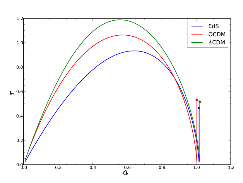
In Fig. 1, we show the evolution of the profile as a function of $a$ for three different cosmological models: EdS, Open CDM with $\Omega_{\rm m}=0.25$ and $\Lambda$CDM with $\Omega_{\rm m}=0.25$ and $\Omega_{\Lambda}=0.75$. Note that in this paper $\Lambda$CDM always refers to this model. The mass of the halo is chosen to be $2\times 10^{13}\,M_{\odot}{h}^{-1}$. The collapse threshold at $z=0$ is set to be $\delta_{\rm c}=1.68$ and extrapolated to the initial time using the linear growth factor for the corresponding cosmology. The initial conditions are set using Eq. 8 and 9. Nonetheless, we still find that we need to choose $a_{*}$ to be sufficiently small ($a_{*}=0.01$ here) to reduce the effects of transients. For example when $a_{*}=0.02$ is chosen instead, we find that the collapse epochs are increased by a few per cent compared to the ones shown. We emphasize that this is because we set up the initial conditions using linear theory, and the transients can be further suppressed using higher order perturbation theory. This is analogous to setting up initial conditions in simulations using 2LPT Scoccimarro (1998); Crocce et al. (2006). Although these cosmologies are rather different, the final collapse epochs are very similar as long as the correct linear growth factor is used to set $\bar{\delta}_{*}$. In other words the collapse threshold is insensitive to the cosmological model Eke et al. (1996). However, the intermediate stages of collapse are quite different among these models. Thus this suggests that we need to solve the model explicitly in order to follow the evolution of the halo profile accurately. We also indicate in Fig. 1 the virial size after the collapse. For EdS and OCDM, it is computed using Eq. 6, while for $\Lambda$CDM we use Eq. 7 with $\Delta_{\rm v}=500$.

Figure 1: The evolution of the halo profile in three different cosmological models EdS (blue), OCDM with $\Omega_{\rm m}=0.25$ (red) and $\Lambda$CDM with $\Omega_{\rm m}=0.25$ and $\Omega_{\rm m}=0.75$ (green). The virial size is indicated as a dot after the collapse.

To illustrate the evolution of the profile, we further assume that the initial halo profile is described by a top-hat profile, and in Fourier space, it reads

$$W_{\rm TH}(\kappa)=\frac{3}{\kappa^{3}}(\sin\kappa-\kappa\cos\kappa).$$ (12)

Top-hat profile is a good approximation at high redshifts. In SC with top-hat perturbation, the top-hat shape is preserved during evolution. The only part that changes is the width of the window. On the other hand, the Eulerian virialized spherical halo profile is well described by the NFW profile Navarro et al. (1996). This means that a top-hat window of perturbation cannot evolve to the NFW-like profile. We will see in Sec. II.2 that the halo profile measured from simulation goes from one resembling top-hat to an NFW-like profile as the redshift decreases.

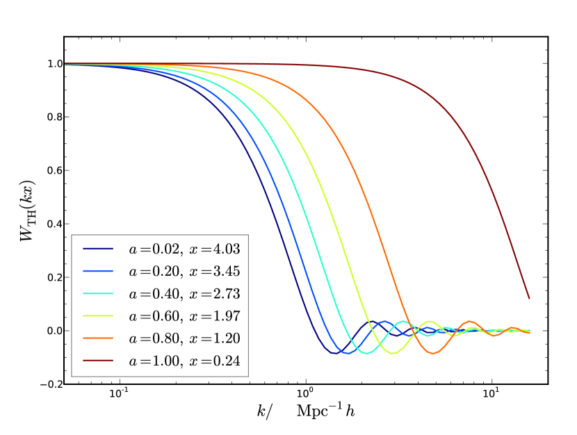
In Fig. 2, we show the evolution of $W_{\rm TH}(kx)$ for a series of values of the comoving size $x$ at different time $a$. We start with $x_{*}=4.07\,\mathrm{Mpc}\,h^{-1}$ at $z_{*}=99$, and the size of the spherical shell is then evolved according to Eq. 1. We have adopted a flat $\Lambda$CDM model with $\Omega_{\Lambda}=0.75$, and $\delta_{\rm c}=1.68$. Note that although the physical size $r$ first expands and then collapses as in Fig. 1, the comoving size $x$ is always decreasing as the effect of expansion is removed. At $a=1$, the shell has not fully collpased yet. As we will see later on, we are mainly interested in the low $k$ part of the window, thus to a very good approximation, the window is essentially 1 up to $k\sim 3\,\mathrm{Mpc}^{-1}\,h$ at the present time. In this plot we have not substituted the halo size at $a=1$ with the virial size. Most of time in the paper, the sudden change during virialization does not matter as it occurs almost instantaneous for our purpose. From now on, the SC model refers the one obtained by evolving an initially top-hat perturbation using Eq. 1.

Figure 2: The evolution of the top-hat window, $W_{\rm TH}(kx)$ for a suite of scale factor $a$. The comoving size $x$ of the spherical shell is computed using the SC model.

II.2 Measurement of the profile evolution from simulations

Figure 3: The halo profile at $z=0$, 0.34, 0.73, 0.97, 1.5, and 49. The Eulerian profile is at $z=0$, and the proto-halo profiles are obtained by tracing the particles in the Eulerian halo to higher redshifts, $z_{\rm L}$. Results from halos of mass ranging from $6.9\times 10^{13}\,M_{\odot}{h}^{-1}$ to $1.3\times 10^{15}\,M_{\odot}{h}^{-1}$ are shown. The density is normalized with respect to the mean comoving density of matter, $\bar{\rho}_{\rm m}$ and the radial distance $r$ is normalized with respect to the Eulerian virial size of the halo, $r_{\rm v}$. The results are from the Oriana simulations.

Figure 4: Same as Fig. 3, except in Fourier space. The halo profile is normalized such that it approaches 1 as $k$ tends to 0.

In this section, we will measure the evolution of halo profile from $N$-body simulation. Starting from Eulerian halos, such as those at $z=0$, we trace the particles in the Eulerian halo back in time to construct the proto-halos at earlier times. The position of the proto-halo at redshift $z$ is defined by the CM of its constituent particles at redshift $z$. We will consider proto-halos at various redshifts.

Before presenting the numerical results we would like to first outline the details of the $N$-body simulation used here. We shall use the Oriana and Carmen simulations in the LasDamas project. In these simulations, a flat $\Lambda$CDM model with the cosmological parameters, $\Omega_{\rm m}=0.25$, $\Omega_{\Lambda}=0.75$ and $\sigma_{8}=0.8$ are adopted. The transfer function is output from CMBFAST Seljak and Zaldarriaga (1996). The initial conditions are Gaussian with spectral index being 1. The initial displacement fields are created using 2LPT Crocce et al. (2006) at $z=49$. The simulations are evolved using the code Gadget2 Springel (2005). In the Oriana simulations, there are $1280^{3}$ particles in a cubic box of size 2400 $\,\mathrm{Mpc}\,h^{-1}$, while for Carmen simulation there are $1120^{3}$ particles in a box of size $1000\,\mathrm{Mpc}\,h^{-1}$. Thus the particle masses are $4.57\times 10^{11}$ and $4.94\times 10^{10}\,M_{\odot}{h}^{-1}$ for Oriana and Carmen respectively. We shall use five realizations for Oriana and seven for Carmen. The halos are obtained using Friend-of-Friend halo finder. For Oriana, the linking length $b=0.156$ is used, while $b=0.2$ for Carmen. To resolve the halo better, we use halos with at least 150 particles. Although the Carmen simulations have better mass resolution than Oriana, we find that their results are quite similar. To avoid redundancy, most of the time, we only show results from Oriana.

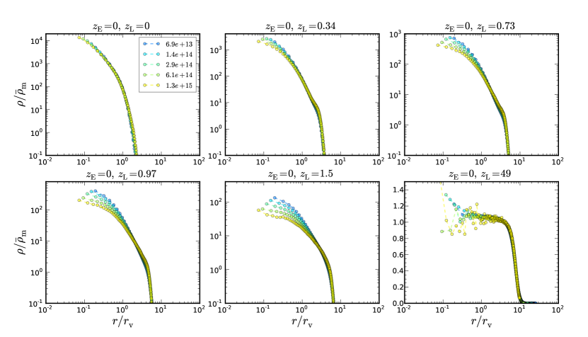
In Fig. 3, we show the halo profile at redshifts, $z=0$, 0.34, 0.73, 0.97, 1.5, and 49. The halo profile is obtained by stacking the halos in the same mass bin together and spherically averaged to get the spherically symmetric profile. In this plot, the Eulerian halo is at $z=0$ and the proto-halos at higher redshifts are constructed from the Eulerian ones. We find that when the size of halos of different masses normalized by their corresponding virial size, they coincide well with each other. We computed $r_{\rm v}$ using $\Delta_{\rm v}=500$ although this is immaterial to our purpose here.

Note that for redshift $z=0$, the halos are in fact in the Eulerian space. The virialized spherical Eulerian halo profile at low redshift is well fitted by the NFW profile. However, the halos used to construct this profile are carefully selected, see e.g. Navarro et al. (1996); Neto et al. (2007). These halos are constructed using spherical overdensity finder and they are chosen to be spherically symmetric and in a relaxed state without signatures of recent mergers. Here we use all the halos obtained from the halo finder without further screening. We find that our Eulerian profile is reasonably well fitted by the NFW profile, but we also find that the profile close to the virial radius drops faster than $r^{-3}$, the scaling of the NFW profile near virial radius. Using the NFW profile, one can show that the Eulerian profile is approximately universal in the variable $r/r_{\rm v}$ for different masses because of the fact that the concentration only weakly depends on the mass of the halo Cooray and Sheth (2002).

The deviation of the proto-halo profile from the NFW profile increases as the redshift increases. At $z=49$, the proto-halo profile corresponds to the one in the initial condition of the simulation. Theoretically, the Lagrangian profile is often assumed to be a top-hat. In Chan et al. (2015), it is found to be in between a Gasussian and a top-hat. More precisely, in Fourier space, the Lagrangian profile is well fitted by a product of a Gaussian and a top-hat window. We note that as $z$ increases, there are large deviations in the profile at small $r$ among different halo masses.

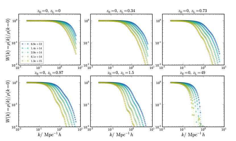
As there is no universal halo profile that can fit the proto-halo profile at various redshifts well, we shall use the numerical profile directly. The profile is Fourier transformed numerically. In the case of the NFW profile, the integration is cut-off at the virial radius $r_{\rm v}$ Cooray and Sheth (2002). In our case, for proto-halos at intermediate redshifts, i.e. in between $z=0$ and $z=49$, it is not clear what the cut-off size should be. Nonetheless, our profile drops rapidly for $r$ greater than a few $r_{\rm v}$, we can take $r$ to be infinity, and the results are unaffected. As the mass of the proto-halo is conserved, we expect the low-$k$ part of the profile at different redshifts to be the same. Numerically, however, this is not always achieved. In each set of simulation, we find that the fractional deviation of the $\rho(k=0)$ across redshifts decreases as the mass of the halo increases. For example, for the lowest mass halo used for Oriana, the fractional deviation of $\rho(k=0)$ is within 10%. This is one of the indications that we should use halos with large number of particles. From now on, we simply normalize the profile so that it is 1 at low $k$. In Fig. 4, we show the Fourier transform of the halo profile for a selection of halo masses. As the redshift $z_{\rm L}$ increases, the size of the proto-halo increases, the window in Fourier space decreases and the low-$k$ plateau shrinks. We also note that there are oscillations in the Fourier transform of the window. It is more visible as the mass of the halo increases because the oscillations are pushed to lower $k$. They are also more prominant as $z_{\rm L}$ increases because the halo profile is more top-hat-like, and hence the wiggles are stronger.

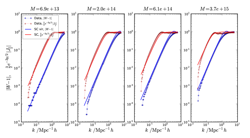
To show the scale-dependence of the window function, in Fig. 5, we plot $|W-1|$ obtained from simulations and the SC model. Absolute value is taken because the $k^{2}$ correction is negative. We have introduced the time variable $y=\ln D$, where $D$ is the linear growth factor (defined by Eq. 16). It is normalized such that $y=0$ at $z_{*}=49$. As we will see in next section, this time variable is convenient. First at $y=0$, SC model agrees with data well except for the highest mass bin shown ($3.7\times 10^{15}\,M_{\odot}{h}^{-1}$). Unfortunately, we have no simulation data available in the range $0\lesssim y\lesssim 3$, although we expect that the overdensity is still in the expansion stage ($y\lesssim 3$), the SC model should work reasonably well. When the region turns around and collapses, we expect the SC model to fail to describe the simulation data accurately. In fact, during the turn-around and collapse phase, the SC results are larger than the simulation data. We also note that for various values of $k$ shown, the agreement between the SC model and the data is qualitatively smiliar. In Fig. 6 we show the corresponding results obtained using the Carmen simulations. In this plot, the Eulerian halos are at $z=0$ and proto-halos are constructed at $z=0.13$, 0.52, 0.97 and 49. Although Carmen has better mass resolution, the results are quite similar to those obtained from Oriana. Overall, the agreement between the simulation results and SC model is reasonable.

Figure 5: The function $|W-1|$ as a function of $y$, obtained from simulations (filled circles) and SC model (solid line). Results from four mass bins of mass $6.9\times 10^{13}$, $2.0\times 10^{14}$, $6.1\times 10^{14}$, and $3.7\times 10^{15}\,M_{\odot}{h}^{-1}$ are shown (from left to right). For each mass bin, $|W(k,y)-1|$ at six different $k$’s are plotted. The data is from Oriana.

Figure 6: Similar to Fig. 5, except for Carmen.

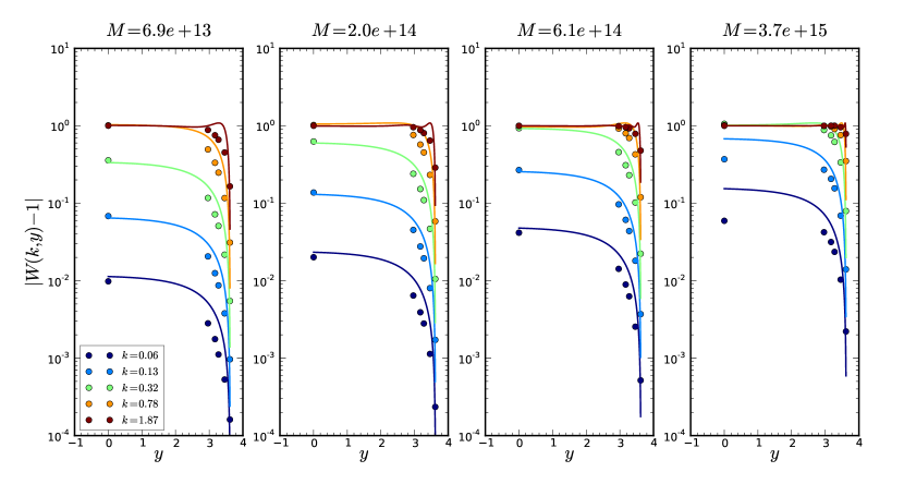
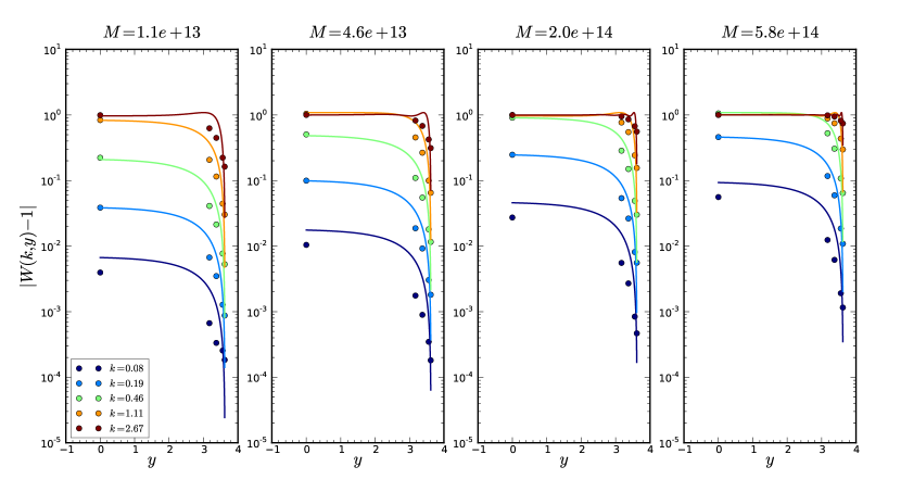
The SC model only works qualitatively at late time. After all, in SC the halo profile shape does not change, but for real halos the halo profile shape does change. In Engineer et al. (2000), a modified SC model that tries to overcome the jump at the final virialization stage was proposed. The model joins smoothly to the final virial scale at the expense of two additional free parameters. The modified model is valid only when the density is high as it is an expansion in $1/\delta$. Nonetheless, using these additional parameters, one may get a profile evolution history, especially the part from turn-around to collapse, to agree with the simulation results better. Another potential way to improve the modelling is to use ellipsoidal model Peebles (1980); Bond and Myers (1996); Shen et al. (2006); Mo et al. (2010). For example, the halo mass function motivated by the ellipsoidal collapse improves the agreement with simulation Sheth et al. (2001) compared to the spherical Press-Schechter one. The halo collapse threshold is also better modelled by the ellipsoidal collapse model Robertson et al. (2009). However, as the halo profile considered here is spherically averaged, one still need to average over the ellipsoidal profile to get the spherically symmetric one. On the data side, we hope to get the data to fill the gap in between 0 and 3 in future. As we see the model does not work very well, in practice it will be useful to come up with a parametrized form for the evolution of the profile. Also the paramertized form of halo can be used to improve the halo model. In the standard halo model one assumes that all the matter exists within halos, and the virialized halo profile is used, such as the NFW profile for halos Cooray and Sheth (2002). However at higher redshift, virialized halos are rare, and this assumption is not justified. One can improve the halo model using the proto-halo profile instead.

III Bias with profile corrections

We shall apply the fluid approximation to model the evolution of the dark matter and the galaxy field. The fluid approximation enable one to derive the nonlocal bias parameters Fry (1996); Chan et al. (2012); Baldauf et al. (2012) which results in better modelling of the halo power spectrum and bispectrum Chan et al. (2012); Baldauf et al. (2012); Saito et al. (2014); Biagetti et al. (2014b) and halo 3-point function Bel et al. (2015). In this paper we use halo and galaxy interchangeably. For dark matter, we will use the standard perturbation theory (SPT) results (see Bernardeau et al. (2002) for a review). In this framework, the evolution of the density contrast of the galaxy, $\delta_{\rm g}$, and its velocity divergence $\theta_{\rm g}$ are governed by the continuity equation and the Euler equation

$$\frac{\partial\delta_{\rm g}}{\partial\tau}+\theta_{\rm g} = -\int d^{3}k_{1}d^{3}k_{2}\delta_{\rm D}(\mathbf{k}-\mathbf{k}_{12})\alpha(\mathbf{k}_{1},\mathbf{k}_{2})\theta_{\rm g}(\mathbf{k}_{1})\delta_{\rm g}(\mathbf{k}_{2}),$$ (13)

$$\frac{\partial\theta_{\rm g}}{\partial\tau}+\mathcal{H}\theta_{\rm g}+\frac{3}{2}\mathcal{H}^{2}\Omega_{\rm m}W\delta = -\int d^{3}k_{1}d^{3}k_{2}\delta_{\rm D}(\mathbf{k}-\mathbf{k}_{12})\beta(\mathbf{k}_{1},\mathbf{k}_{2})\theta_{\rm g}(\mathbf{k}_{1})\delta_{\rm g}(\mathbf{k}_{2}),$$ (14)

where $\tau$ is the conformal time, $\mathcal{H}$ is the conformal Hubble parameter $d\ln a/d\tau$, $\mathbf{k}_{12}$ denotes $\mathbf{k}_{1}+\mathbf{k}_{2}$, and $\alpha$ and $\beta$ are the coupling kernels

$$\alpha(\mathbf{k}_{1},\mathbf{k}_{2})=\frac{\mathbf{k}_{12}\cdot\mathbf{k}_{1}}{k_{1}^{2}},\quad\beta(\mathbf{k}_{1},\mathbf{k}_{2})=\frac{k_{12}^{2}\mathbf{k}_{1}\cdot\mathbf{k}_{2}}{2k_{1}^{2}k_{2}^{2}}.$$ (15)

Here $\Omega_{\rm m}$ is the density parameter of matter.

Eq. 13 and 14 are similar to the fluid equations widely adopted for modeling the evolution of multiple components Somogyi and Smith (2010); Elia et al. (2011); Bernardeau et al. (2012); Chan et al. (2012), except with the window function $W$, which is central to the results in this paper. We also note that in Baldauf et al. (2014), a similar modification of the Euler equation was proposed, in which the authors argued the forced for halos should be biased. However, the physical origin of this modification and its form are quite different from that in Baldauf et al. (2014). Another important difference from Baldauf et al. (2014); Biagetti et al. (2014a) is that we do not impose the peak constraint in the evolution equations. The proto-halos after initial identification, they simply evolve following Eq. 13 and 14.

The introduction of $W$ is to model the fact that although $\delta_{\rm g}$ denotes the density contrast of the spatial distribution of the CM of the halos, each individual halo consists of a collection of particles. Thus the force on the CM of the halo should be the average force acting on all the individual particles in the halo. Hence in real space the effective source of the gravitational force for a finite-sized object is $W*\delta$, instead of only $\delta$ at the CM position of the object. In Fourier space, it is given by the product between $W$ and $\delta$ thanks to the convolution theorem. This window function describes the profile of the object. We will use the window function/profile studied in Sec. II.

To simplify Eq. 13 and 14 further, we introduce the new time variable $y=\ln D$ where $D$ is the linear growth factor for the dark matter satisfying the equation

$$\frac{d^{2}D}{d\tau^{2}}+\mathcal{H}\frac{dD}{d\tau}-\frac{3}{2}\mathcal{H}^{2}\Omega_{\rm m}D=0.$$ (16)

We note that $f^{2}\approx\Omega_{\rm m}$, with $f=d\ln D/d\ln a$ is a very good approximation for the epoch that we are interested in Scoccimarro et al. (1998). Using this approximation Eq. 13 and 14 can be written as

$$\frac{\partial\delta_{\rm g}}{\partial y}-\tilde{\theta_{\rm g}} = \int d^{3}k_{1}d^{3}k_{2}\delta_{\rm D}(\mathbf{k}-\mathbf{k}_{12})\alpha(\mathbf{k}_{1},\mathbf{k}_{2})\tilde{\theta_{\rm g}}(\mathbf{k}_{1})\delta_{\rm g}(\mathbf{k}_{2}),$$ (17)

$$\frac{\partial\tilde{\theta_{\rm g}}}{\partial y}+\frac{1}{2}\tilde{\theta_{\rm g}}-\frac{3}{2}W\delta = \int d^{3}k_{1}d^{3}k_{2}\delta_{\rm D}(\mathbf{k}-\mathbf{k}_{12})\beta(\mathbf{k}_{1},\mathbf{k}_{2})\tilde{\theta_{\rm g}}(\mathbf{k}_{1})\tilde{\theta_{\rm g}}(\mathbf{k}_{2}),$$ (18)

where $\tilde{\theta_{\rm g}}$ denotes $\theta_{\rm g}/(-f\mathcal{H})$. In the rest of the paper, we shall abuse the notation and simply use $\theta$ and $\theta_{\rm g}$ to denote $\theta/(-f\mathcal{H})$ and $\theta_{\rm g}/(-f\mathcal{H})$ respectively.

In the following subsections, we will solve Eq. 17 and 18 to linear and second order respectively to reveal the effects of the window function on the bias parameters. In Chan et al. (2012), the continuity and Euler equation of the galaxy field together with the other two equations for dark matter were written in a concise form, and hence a general perturbative solution was obtained using the transient formalism Scoccimarro (1998), thanks to the fact that the coefficients of the equations are not explicitly time-dependent. However, $W$ is time-dependent as we see in Sec. II. Here we will solve Eq. 17 and 18 directly.

III.1 Linear biases

We start from the linearized version of Eq. 17 and 18

$$\partial_{y}\delta_{\rm g}^{(1)} = \theta_{\rm g}^{(1)},$$ (19)

$$\partial_{y}\theta_{\rm g}^{(1)}+\frac{1}{2}\theta_{\rm g}^{(1)} = \frac{3}{2}W\delta^{(1)},$$ (20)

where the superscript (1) emphasizes that the field is linear. We have suppressed the explicit $\mathbf{k}$-dependence.

III.1.1 Velocity

Figure 7: Evolution of the linear velocity bias with static window (dashed) and that with window given by SC (solid). Three redshifts are shown $z=5$ (blue), 1 (red) and 0 (green). The case with static window is almost constant (thus some of the curves are covered by the blue curves), while the evolving window case gives decaying, but not negligible $b_{\rm v}$.

Figure 8: The integrand $|j_{\frac{3}{2}}|$ as a function of $y$ for various values of $k$, obtained from simulation data (filled circles). The results from the SC (solid) and the static window (dashed) are also shown. The simulation data is from Oriana.

Figure 9: The comparison of the contribution to $k^{2}$ from $|W-1|$ (blue) and $\frac{3}{2}e^{-\frac{3y}{2}}|J_{\frac{3}{2}}|$ (red), which is the main contribution to $k^{2}$ correction in the velocity bias in Eq. 28. The results from simulations (symbol) and SC (solid line) are shown. The simulation data is from Oriana. For $W-1$ from SC, we have used $r_{\rm v}$ computed with $\Delta_{\rm v}=500$. The quantities are evaluated are $z=0$.

We will work on the Euler equation first because it depends only on $\theta_{\rm g}^{(1)}$. Integrating Eq. 20 in terms of $W$ and $\delta^{(1)}$, we get

$$\theta_{\rm g}^{(1)}(y)=\theta_{\rm g}^{*(1)}e^{-\frac{y}{2}}+\frac{3}{2}\int_{0}^{y}dy^{\prime}W(y^{\prime})\delta^{(1)}(y^{\prime})e^{-\frac{1}{2}(y-y^{\prime})}.$$ (21)

As we mentioned before, in this paper, we use star “*” to denote a quantity at some initial time. Thus $\theta_{\rm g}^{*(1)}$ is the velocity divergence of the galaxy at the initial time. For convenience, we define the function $I_{n}$ as

$$I_{n}(y)=\int_{0}^{y}dy^{\prime}W(y^{\prime})e^{ny^{\prime}},$$ (22)

thus we have

$$\theta_{\rm g}^{(1)}(y)=\theta_{\rm g}^{*(1)}e^{-\frac{y}{2}}+\frac{3}{2}\delta_{*}^{(1)}e^{-\frac{y}{2}}I_{\frac{3}{2}},$$ (23)

where we have used the SPT result

$$\delta^{(1)}(y)=\delta_{*}^{(1)}e^{y}.$$ (24)

Note that we have normalized the linear growth factor to be 1 at the initial time so that $y_{*}=0$.

The linear velocity bias $b_{\rm v}$ then is given by

$$b_{\rm v}(y) \equiv \frac{\theta_{\rm g}^{(1)}(y)}{\theta^{(1)}(y)}$$ (25)

$$= b_{\rm v}^{*}e^{-\frac{3y}{2}}+\frac{3}{2}e^{-\frac{3}{2}y}I_{\frac{3}{2}},$$

where we have used

$$\theta^{(1)}(y)=\theta_{*}^{(1)}e^{y}=\delta_{*}^{(1)}e^{y}.$$ (26)

Correspondingly the initial linear velocity bias $b_{\rm v}^{*}$ is defined as

$$b_{\rm v}^{*}\equiv\frac{\theta_{\rm g}^{*(1)}}{\theta_{*}^{(1)}}.$$ (27)

In Fourier space, the window function approaches 1 at low $k$, thus it is convenient to express the integral in Eq. 25 in terms of $W-1$. Hence we have instead

$$b_{\rm v}=1+(b_{\rm v}^{*}-1)e^{-\frac{3y}{2}}+\frac{3}{2}e^{-\frac{3y}{2}}J_{\frac{3}{2}}(y),$$ (28)

where $J_{n}$ denotes the integral

$$J_{n}(y)=\int_{0}^{y}dy^{\prime}[W(y^{\prime})-1]e^{ny^{\prime}}.$$ (29)

The advantage of introducing $J_{n}$ is that it gives at least $k^{2}$ order correction, thus it represents the genuine halo profile correction. The first two terms in Eq. 28 are the velocity bias evolution obtained in Chan et al. (2012), and the last term is new, which arises from the halo profile. In the limit of large $y$, the profile correction does not vanish, instead $b_{\rm v}$ tends to $1+\frac{3}{2}e^{-\frac{3y}{2}}J_{\frac{3}{2}}(y)$. If we assume that the window is static, we get $W$.

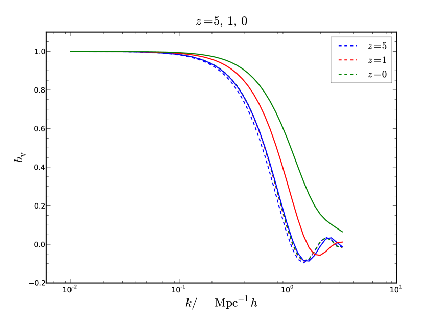
In Fig. 7, we plot $b_{\rm v}$ at $z=5$, 1 and 0. To set the initial condition, $b_{\rm v}^{*}$ at $z_{*}=49$, we borrow the results from peak theory Desjacques and Sheth (2010)

$$b_{\rm v}^{*}=\Big{(}1-\frac{s_{0}}{s_{1}}k^{2}\Big{)}W_{\rm G}(kR_{\rm G}),$$ (30)

where $W_{\rm G}$ denotes the Gaussian window function and $s_{n}$ is the spectral moment defined as

$$s_{n}=4\pi\int dkk^{2(n+1)}P(k)W_{\rm G}^{2}(kR_{\rm G}).$$ (31)

Let’s clarify the reason that we set the initial conditions using the peak theory even though we dispute about its prediction at late time. Various studies, e.g. Elia et al. (2002); Chan et al. (2015) show that the density and velocity cross power spectrum between halo and matter in the Lagrangian space can be well fitted by the functional form motivated by the peak theory. Thus one may think that here we only use an established fact from simulations. However we argue that the subsequent evolution can be modelled by the simple fluid approximation augmented with the window function.

In the plot, as an example we will consider halo of mass $2\times 10^{13}\,M_{\odot}{h}^{-1}$. We map the top-hat window size to the Gaussian window size using the relation $R_{\rm G}=R_{\rm TH}/\sqrt{5}$. We compare the case when the window is static, with the window size given by the Lagrangian size and the case in which the window size is evolved by the SC model. The difference in treatment is only in $J_{\frac{3}{2}}$ in Eq. 28. We note that when the window is static, the resultant $b_{\rm v}$ is almost constant over time. However, when the window is evolved by the SC model, $b_{\rm v}$ decays over time, but it is not negligible at late time.

Although we have used Eq. 30, as in the initial condition, the contributions from the initial scale-dependent part is small compared to the ones due to $J_{n}$, even if we have used $b_{\rm v}^{*}=1$, we find that the results are quite similar to that in Fig. 7. This highlights that the scale dependence of $b_{\rm v}$ is mainly driven by the late time halo profile.

In the literature, the velocity bias is often associated with $k^{2}$ correction to both the density and velocity biases, e.g. these $k^{2}$ corrections can be derived from the peak model Desjacques and Sheth (2010). In Desjacques et al. (2010), Zel’dovich approximation was used to displace the peaks to the Eulerian space, and they found that the velocity bias remains constant over time. The numerical measurement seemed to be in favour of the peak model result Baldauf et al. (2014). Here we show that taking into account that halos are composite objects there is significant $k^{2}$-correction to the velocity bias and it does not decay away over time. When the static window is used, we also find that $b_{\rm v}$ reduces to $W$ in the long term limit. However, when the evolving SC model is applied, the velocity bias is not constant, as can be seen from Fig. 7. Even in the static window limit, our result ($W$) is still different from Desjacques et al. (2010), which gets $Wb_{\rm v}^{\rm pk}$ instead. The reason for this difference is that we do not impose the peak constraint in proto-halo evolution Biagetti et al. (2014a). These differences can be used to differentiate these two models.

Alternatively we can express the linear bias parameters in terms of the time derivative of the profile. Integrating the integral in Eq. 25 by parts, $b_{\rm v}$ can be written as

$$b_{\rm v}(y) = W(y)+[b_{\rm v}^{*}-W(0)]e^{-\frac{3}{2}y}$$ (32)

$$- \int_{0}^{y}dy^{\prime}W^{\prime}(y^{\prime})e^{-\frac{3}{2}(y-y^{\prime})},$$

where $W^{\prime}$ denotes $\partial W/\partial y$. This form shows that there are two contributions to the $k^{2}$ correction from the profile, one from $W$ and another from $W^{\prime}$. The contribution from $W$ is simply the trivial smoothing. However, numerically performing derivatives on sparse data can lead to noisy results. Thus we will only use the form in terms of $J_{n}$, such as Eq. 28.

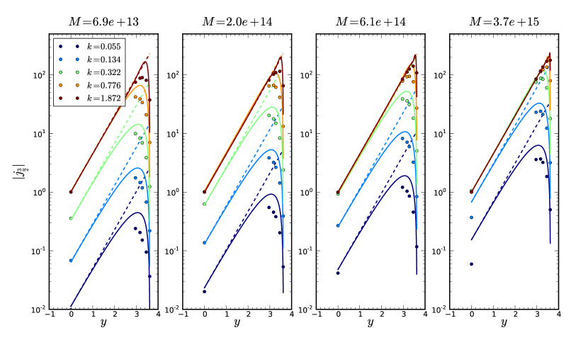
As the velocity bias is mainly generated by $J_{\frac{3}{2}}$ in Eq. 28, to gain insight into which part of the integral of $J_{\frac{3}{2}}$ contributes most, we plot the integrand of $J_{\frac{3}{2}}$, $j_{\frac{3}{2}}$

$$j_{\frac{3}{2}}(y)=e^{\frac{3}{2}y}\Big{(}W(y)-1\Big{)}$$ (33)

in Fig. 8. Again, in the range $0<y\lesssim 3$, there are no data available. We also show the prediction from the SC model. SC predicts that the contribution to the results in that range is small, while the contribution around $y\sim 3$ is the largest. However, we note that the SC results often overshoots in this range. We also show the results obtained with the static window. Static window approximation is good for $y\lesssim 2$, but it overestimates the results for $y\gtrsim 3$.

As both the window function $W$ and the time integral $J_{\frac{3}{2}}$ contribute to leading $k^{2}$ correction, we would like to compare the magnitude of these terms. In Fig. 9, we compare $k^{2}$ contributions from $|W-1|$ and $\frac{3}{2}e^{-\frac{3y}{2}}|J_{\frac{3}{2}}|$ using both the numerical results and the SC model. The results are for $z=0$. The SC model gives quite good description of the results from the data. In particular, the value of $\frac{3}{2}e^{-\frac{3y}{2}}|J_{\frac{3}{2}}|$ from numerical window and the SC model agrees quite well.

For the SC result for $|W-1|$, we have compared a few prescriptions for the size of the window. Although at $z=0$ the size has not yet collapsed exactly to zero, using such a value gives the magnitude of $W-1$ much smaller than the simulation results. We have tried using Eq. 7 with $\Delta_{\rm v}=200$, 380 and 500, and $\Delta_{\rm v}=500$ gives the best agreement with simulations. In Fig. 9 we have shown the results obtained using $\Delta_{\rm v}=500$. In passing, if we simply use Eq. 6, which is strictly only for matter-dominated universe, we get the results very similar to those from $\Delta_{\rm v}=380$. We have cross-checked the results using Carmen, and they are consistent with those from Oriana.

We note that recently there are reports of measurements of velocity bias at late time Baldauf et al. (2014); Jennings et al. (2014); Zheng et al. (2014a). In Baldauf et al. (2014), the momentum was measured, and they found that the model with $b_{\rm pk}$ arised due to the peak constraint seems to fit the data better at high redshift such as $z=20$ than the evolution model without it. At such high redshifts, the effect of the profile evolution is small as can be seen from Fig. 7. Thus if confirmed, this would shows that the profile correction would not be the dominant effect of the velocity bias seen in simulations. In the study of Zheng et al. (2014a), velocity bias was measured with sampling bias correction applied. They found that the velocity bias at $k\sim 0.08\,\mathrm{Mpc}^{-1}\,h$ is slightly positive, with $b_{\rm v}\sim 1.01$. In our model, velocity bias can only be negative in the mildly nonlinear regime. However, as the number density of halos is low and halos are more inhomogeneously distributed in Eulerian space, thus it is hard to get an accurate volume weighted measurement. It is not clear that these measurements are free of artifacts. Thus we will keep these in mind and hope to report our own numerical comparison in future.

III.1.2 Density

Figure 10: Evolution of the linear density bias with static window (dashed) and evolving window given by the SC (solid). Three redshifts are shown: $z=5$ (blue), 1 (red) and 0 (green).

Figure 11: Same as Fig. 10, except the scale independent initial conditions $b_{1}^{*}=b_{\nu}$ and $b_{\rm v}^{*}=1$ are assumed.

We now turn to the density bias. Plugging Eq. 21 into Eq. 19, we have

$$\delta_{\rm g}^{(1)}(y) = \delta_{\rm g}^{*(1)}+2\theta_{\rm g}^{*(1)}(1-e^{-\frac{y}{2}})$$ (34)

$$+ \frac{3}{2}\delta_{*}^{(1)}\int_{0}^{y}dy^{\prime}e^{-\frac{y^{\prime}}{2}}I_{\frac{3}{2}}(y^{\prime}).$$

It is useful to note that

$$\int_{0}^{y}dy^{\prime}e^{ay^{\prime}}I_{b}(y^{\prime})=\frac{1}{a}[e^{ay}I_{b}(y)-I_{a+b}(y)].$$ (35)

Using Eq. 35, we can simplify Eq. 34 to

$$\delta_{\rm g}^{(1)}(y)=\delta_{\rm g}^{*(1)}+2\theta_{\rm g}^{*(1)}(1-e^{-\frac{y}{2}})-3\delta_{*}^{(1)}[e^{-\frac{y}{2}}I_{\frac{3}{2}}-I_{1}].$$ (36)

Thus the linear density bias is given by

$$b_{1}(y) \equiv \frac{\delta_{\rm g}^{(1)}(y)}{\delta^{(1)}(y)}$$ (37)

$$= b_{1}^{*}e^{-y}+2b_{\rm v}^{*}e^{-y}(1-e^{-\frac{y}{2}})$$

$$\quad-3e^{-y}(e^{-\frac{y}{2}}I_{\frac{3}{2}}-I_{1}),$$

where $b_{1}^{*}$ is defined as

$$b_{1}^{*}\equiv\frac{\delta_{\rm g}^{*(1)}}{\delta_{*}^{(1)}}.$$ (38)

Or in terms of $J_{n}$ using $I_{n}=J_{n}+(e^{ny}-1)/n$, we have

$$b_{1}(y) = 1+(b_{1}^{*}+2b_{\rm v}^{*}-3)e^{-y}+2(1-b_{\rm v}^{*})e^{-\frac{3y}{2}}$$ (39)

$$+ 3e^{-y}J_{1}-3e^{-\frac{3y}{2}}J_{\frac{3}{2}}.$$

The first line in Eq. 39 is the same as the time evolution of linear density bias obtained in Chan et al. (2012), while the second line results from the halo profile correction. Unlike the decaying terms in the first line, they do not decay away. In the long term limit, $b_{1}$ reduces to $1+3e^{-y}J_{1}-3e^{-\frac{3y}{2}}J_{\frac{3}{2}}$. If we assume that the window is static, we get $b_{1}=W$ in the long term limit.

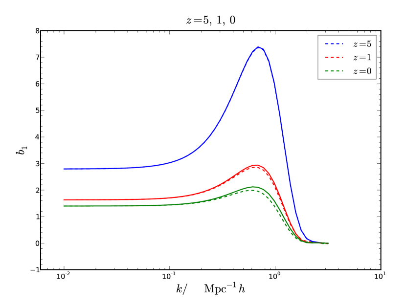
In Fig. 10, the evolution of the linear density bias is plotted. Again we use the form of the initial condition motivated by the peak theory Desjacques and Sheth (2010)

$$b_{1}^{*}=(b_{\nu}+b_{\zeta}k^{2})W_{\rm G}(kR_{\rm G}).$$ (40)

We take $R_{\rm G}$ corresponding to halo of mass $2\times 10^{13}\,M_{\odot}{h}^{-1}$. Instead of using the peak theory results, we take $b_{\nu}=15.9$ and $b_{\zeta}=40.0\,(\,\mathrm{Mpc}\,h^{-1})^{2}$, which are obatined from measurement of the initial cross power spectrum Chan et al. (2015). Both the results from the static window and SC evolving window are shown, however, the differences are very small.

The initial condition term $(b_{1}^{*}+2b_{\rm v}^{*}-3)e^{-y}$, especially due to $b_{1}^{*}$, is important at low $k$. In fact, at low $k$, it gives the decay of linear bias Fry (1996) . The term due solely to $b_{\rm v}^{*}$, $2(1-b_{\rm v}^{*})e^{-3y/2}$ is negligible in the whole range of $k$ shown. The sum of the two profile correction terms, $J_{1}$ and $J_{\frac{3}{2}}$ gives small overall correction. That is also the reason why the static and evolving window gives almost identical results. The reason that the profile correction term $J_{n}$ gives much more significant effect for $b_{\rm v}$ than for $b_{1}$ is that unlike the case of $b_{\rm v}$, $b_{1}$ at late time is still dominated by the reminant effect of $b_{1}^{*}$ because the magnitude of $b_{1}^{*}$ is much larger than that of $b_{\rm v}^{*}$.

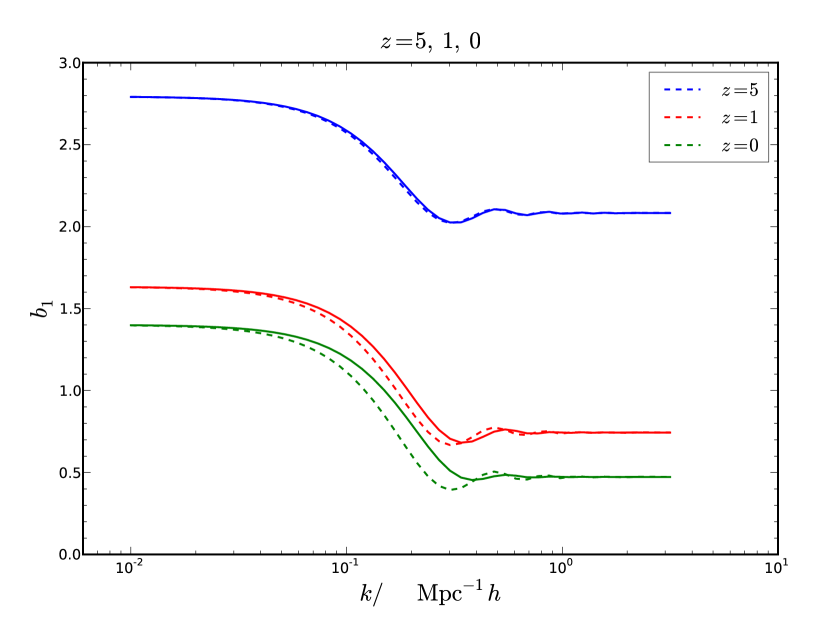
Unlike the case $b_{\rm v}$, the magnitude of the scale-dependent part of $b_{1}^{*}$ in Eq. 40 is significant compared to other contributions. To highlight its effect, we plot the results when the initial bias is scale-independent, i.e. $b_{1}^{*}=b_{\nu}$ and $b_{\rm v}^{*}=1$ in Fig. 11. This plot shows that the bump in Fig. 10 around $k\sim 0.7\,\mathrm{Mpc}^{-1}\,h$ is due to the large magnitude of the initial $b_{\zeta}k^{2}$ term. The low $k$ plateau is due to $b_{\nu}$ from initial condition and the scale-dependent transition comes from $J_{1}$ and $J_{\frac{3}{2}}$ terms.

III.2 Second order biases

To second order, Eq. 17 and 18 become

$$\frac{\partial\delta_{\rm g}^{(2)}}{\partial y}-\theta_{\rm g}^{(2)} = \int d^{3}k_{1}d^{3}k_{2}\delta_{\rm D}(\mathbf{k}-\mathbf{k}_{12})\alpha(\mathbf{k}_{1},\mathbf{k}_{2})\theta_{\rm g}^{(1)}(\mathbf{k}_{1})\delta_{\rm g}^{(1)}(\mathbf{k}_{2}),$$ (41)

$$\frac{\partial\theta_{\rm g}^{(2)}}{\partial y}+\frac{1}{2}\theta_{\rm g}^{(2)}-\frac{3}{2}W\delta^{(2)} = \int d^{3}k_{1}d^{3}k_{2}\delta_{\rm D}(\mathbf{k}-\mathbf{k}_{12})\beta(\mathbf{k}_{1},\mathbf{k}_{2})\theta_{\rm g}^{(1)}(\mathbf{k}_{1})\theta_{\rm g}^{(1)}(\mathbf{k}_{2}).$$ (42)

We shall solve Eq. 41 and 42 perturbatively to obtain $\delta_{\rm g}^{(2)}$ and $\theta_{\rm g}^{(2)}$.

III.2.1 Velocity

We will start from Eq. 42 to compute $\theta_{\rm g}^{(2)}$ first. Using the dark matter SPT result

$$\delta^{(2)}(y)=e^{2y}\delta^{(2)}_{*}.$$ (43)

and Eq. 23, we can integrate Eq. 42 to get

$$\theta_{\rm g}^{(2)}(y) = \theta_{\rm g}^{*(2)}e^{-\frac{y}{2}}+\frac{3}{2}\delta_{*}^{(2)}e^{-\frac{y}{2}}I_{\frac{5}{2}}(y)+\int d^{3}k_{1}d^{3}k_{2}\delta_{\rm D}(\mathbf{k}-\mathbf{k}_{12})\beta(\mathbf{k}_{1},\mathbf{k}_{2})$$ (44)

$$\times e^{-\frac{y}{2}}\Big{\{}2(1-e^{-\frac{y}{2}})\theta_{\rm g}^{*(1)}(\mathbf{k}_{1})\theta_{\rm g}^{*(1)}(\mathbf{k}_{2})-\frac{3}{2}\big{[}(e^{-\frac{y}{2}}I_{\frac{3}{2}}(\mathbf{k}_{2})-I_{1}(\mathbf{k}_{2}))\theta_{\rm g}^{*(1)}(\mathbf{k}_{1})\delta_{*}^{(1)}(\mathbf{k}_{2})+(\mathbf{k}_{1}\leftrightarrow\mathbf{k}_{2})\big{]}$$

$$+ \frac{9}{4}\int_{0}^{y}dy^{\prime}e^{-\frac{y^{\prime}}{2}}I_{\frac{3}{2}}(y^{\prime},\mathbf{k}_{1})I_{\frac{3}{2}}(y^{\prime},\mathbf{k}_{2})\delta_{*}^{(1)}(\mathbf{k}_{1})\delta_{*}^{(1)}(\mathbf{k}_{2})\Big{\}}.$$

Replacing $\theta_{\rm g}^{*(1)}$ by $b_{\rm v}^{*}\delta_{*}^{(1)}$ and extrapolating $\delta_{*}^{(1)}$ to the present time, we have

$$\theta_{\rm g}^{(2)}(y) = \theta_{\rm g}^{*(2)}e^{-\frac{y}{2}}+\frac{3}{2}\delta^{(2)}(y)e^{-\frac{5y}{2}}I_{\frac{5}{2}}(y)+\int d^{3}k_{1}d^{3}k_{2}\delta_{\rm D}(\mathbf{k}-\mathbf{k}_{12})K_{\theta 2}(\mathbf{k}_{1},\mathbf{k}_{2})\delta^{(1)}(\mathbf{k}_{1})\delta^{(1)}(\mathbf{k}_{2}),$$ (45)

where $K_{\theta 2}$ is given by

$$K_{\theta 2}(\mathbf{k}_{1},\mathbf{k}_{2}) = e^{-\frac{5y}{2}}\beta(\mathbf{k}_{1},\mathbf{k}_{2})\Big{\{}2(1-e^{-\frac{y}{2}})b_{\rm v}^{*}(\mathbf{k}_{1})b_{\rm v}^{*}(\mathbf{k}_{2})-\frac{3}{2}\big{[}(e^{-\frac{y}{2}}I_{\frac{3}{2}}(\mathbf{k}_{2})-I_{1}(\mathbf{k_{2}}))b_{\rm v}^{*}(\mathbf{k}_{1})+(\mathbf{k}_{1}\leftrightarrow\mathbf{k}_{2})\big{]}$$ (46)

$$+ \frac{9}{4}\int_{0}^{y}dy^{\prime}e^{-\frac{y^{\prime}}{2}}I_{\frac{3}{2}}(y^{\prime},\mathbf{k}_{1})I_{\frac{3}{2}}(y^{\prime},\mathbf{k}_{2})\Big{\}},$$

where $(\mathbf{k}_{1}\leftrightarrow\mathbf{k}_{2})$ is a shorthand for a similar term obtained with $\mathbf{k}_{1}$ and $\mathbf{k}_{2}$ interchanged. To be general, we allow the initial linear biases to be scale-dependent. Note that $K_{\theta 2}$ is already symmetric in $\mathbf{k}_{1}$ and $\mathbf{k}_{2}$, so symmetrization is not required.

In terms of $J_{n}$, $\theta_{\rm g}^{(2)}$ can be expressed as

$$\theta_{\rm g}^{(2)}(y)=\theta_{\rm g}^{*(2)}e^{-\frac{y}{2}}+\int d^{3}k_{1}d^{3}k_{2}\delta_{\rm D}(\mathbf{k}-\mathbf{k}_{12})\mathcal{K}_{\theta 2}(\mathbf{k}_{1},\mathbf{k}_{2})\delta^{(1)}(\mathbf{k}_{1})\delta^{(1)}(\mathbf{k}_{2}),$$ (47)

where $\mathcal{K}_{\theta 2}$ is given by

$$\mathcal{K}_{\theta 2}=T_{F}+T_{G}+T_{b_{\rm v}^{*}}+T_{JJ}+T_{J}.$$ (48)

The five types of terms $T_{F}$, $T_{G}$, $T_{b_{\rm v}^{*}}$, $T_{JJ}$, and $T_{J}$ are given by

$$T_{G} = (1-e^{-\frac{5y}{2}})G_{2}(\mathbf{k}_{1},\mathbf{k}_{2}),$$ (49)

$$T_{F} = \frac{3}{2}e^{-\frac{5y}{2}}J_{\frac{5}{2}}(\mathbf{k})F_{2}(\mathbf{k}_{1},\mathbf{k}_{2}),$$ (50)

$$T_{b_{\rm v}^{*}} = \beta(\mathbf{k}_{1},\mathbf{k}_{2})\Big{\{}2e^{-\frac{5y}{2}}(1-e^{-\frac{y}{2}})b_{\rm v}^{*}(\mathbf{k}_{1})b_{\rm v}^{*}(\mathbf{k}_{2})+e^{-\frac{5y}{2}}(e^{y}+2e^{-\frac{y}{2}}-3)\big{(}b_{\rm v}^{*}(\mathbf{k}_{1})+b_{\rm v}^{*}(\mathbf{k}_{2})\big{)}$$ (51)

$$- 2(e^{-\frac{3y}{2}}-2e^{-\frac{5y}{2}}+e^{-3y})-\frac{3}{2}e^{-3y}\Big{[}\big{(}J_{\frac{3}{2}}(\mathbf{k}_{2})-J_{1}(\mathbf{k}_{2})\big{)}b_{\rm v}^{*}(\mathbf{k}_{1})+(\mathbf{k}_{1}\leftrightarrow\mathbf{k}_{2})\Big{]}\Big{\}},$$

$$T_{JJ} = \beta(\mathbf{k}_{1},\mathbf{k}_{2})e^{-\frac{5y}{2}}\int_{0}^{y}dy^{\prime}e^{-\frac{y^{\prime}}{2}}\frac{9}{4}J_{\frac{3}{2}}(y^{\prime},\mathbf{k}_{1})J_{\frac{3}{2}}(y^{\prime},\mathbf{k}_{2}),$$ (52)

$$T_{J} = \beta(\mathbf{k}_{1},\mathbf{k}_{2})e^{-\frac{5y}{2}}\int_{0}^{y}dy^{\prime}e^{-\frac{y^{\prime}}{2}}\frac{3}{2}(e^{\frac{3y^{\prime}}{2}}-1)\big{(}J_{\frac{3}{2}}(y^{\prime},\mathbf{k}_{1})+J_{\frac{3}{2}}(y^{\prime},\mathbf{k}_{2})\big{)},$$ (53)

where $\mathbf{k}=\mathbf{k}_{12}$, and $F_{2}$ and $G_{2}$ represent the coupling kernels

$$F_{2}(\mathbf{k}_{1},\mathbf{k}_{2})=\frac{5}{7}+\frac{1}{2}\mu\big{(}\frac{k_{1}}{k_{2}}+\frac{k_{2}}{k_{1}}\big{)}+\frac{2}{7}\mu^{2},\quad\quad G_{2}(\mathbf{k}_{1},\mathbf{k}_{2})=\frac{3}{7}+\frac{1}{2}\mu\big{(}\frac{k_{1}}{k_{2}}+\frac{k_{2}}{k_{1}}\big{)}+\frac{4}{7}\mu^{2},$$ (54)

with $\mu=\hat{\mathbf{k}}_{1}\cdot\hat{\mathbf{k}}_{2}$.

As a cross-check, we pause to consider the limit $b_{\rm v}^{*}=1$ and $J_{n}=0$. Then $\mathcal{K}_{\theta 2}$ reduces to $(1-e^{-\frac{5y}{2}})G_{2}$. Note that in this limit $\theta_{\rm g}^{*(2)}e^{-\frac{y}{2}}=\theta^{*(2)}e^{-\frac{y}{2}}=\theta^{(2)}e^{-\frac{5y}{2}}$, thus Eq. 47 reduces to $\theta^{(2)}$ because the galaxy field reduces to the dark matter field. On the other hand, in the long term limit $y\rightarrow\infty$, the transient terms vanish, in particular those arising from $b_{\rm v}^{*}$, and we end up with $G_{2}+T_{F}+T_{JJ}+T_{J}$.

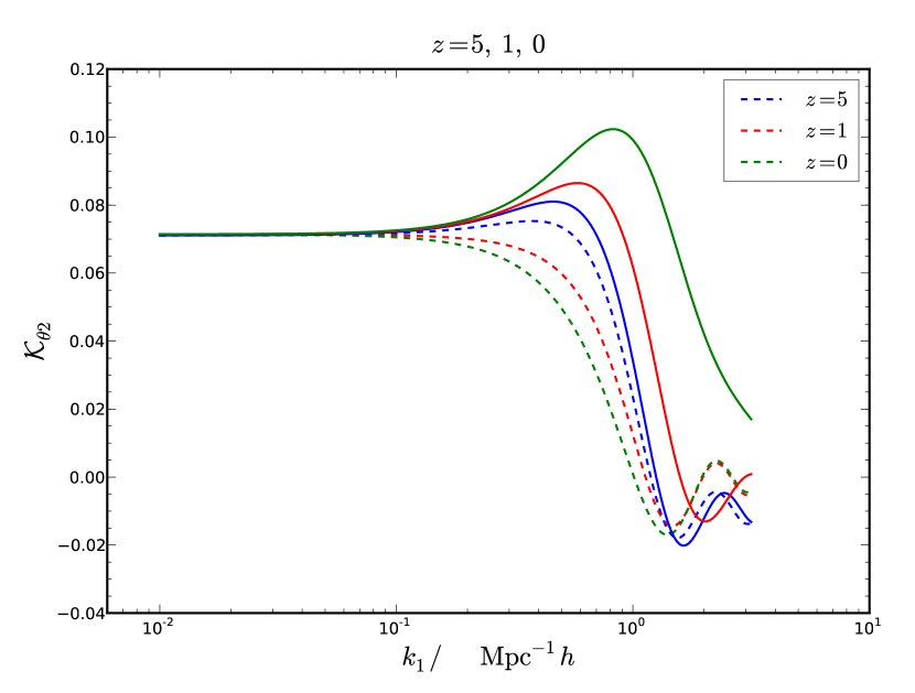
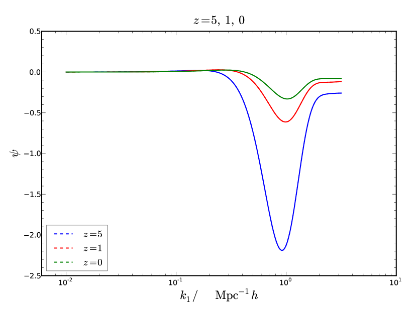
In Fig. 12, we show the evolution of the kernel $\mathcal{K}_{\theta 2}$. In this plot, we have used the same parameters as those in the previous section and have set $k_{1}=k_{2}$ and $\mu=-1/2$, which corresponds to the equilateral triangle configuration. We have compared the case with the static window and the one with SC evolving window, and find that the high $k$ corrections are quite different. In particular, the magnitude of the static one decreases while the evolving one increases over time. When $b_{\rm v}^{*}$ is assumed to be scale-independent instead, the results are similar to Fig. 12, thus we do not show it here.

We now look at the individual components of $\mathcal{K}_{\theta 2}$ in details in this example. At low $k$, the only non-vanishing component is $T_{G}$ and it is (almost) constant for the reshifts shown. The term $T_{F}$ gives negative $k^{2}$ correction and its magnitude is large among all the high $k$ correction terms. The term $T_{J}$ and $T_{JJ}$ are of opposite signs, but the magnitude of $T_{J}$ is slightly larger. In particular, as the leading correction from $T_{JJ}$ is of $k^{4}$, compared to $T_{J}$, it is unimportant for $k\lesssim 0.6\,\mathrm{Mpc}^{-1}\,h$. $T_{F}$ and $T_{J}$ are the largest scale-dependent correction terms, they are of similar magnitude but of opposite signs. The term with $b_{\rm v}^{*}$, $T_{b_{\rm v}^{*}}$ gives small negative contribution, which is negligible compared to the other correction terms. In fact for $k\lesssim 0.6\,\mathrm{Mpc}^{-1}\,h$, the kernel $\mathcal{K}_{\theta 2}$ is well captured by the sum $T_{F}+T_{G}+T_{J}$. This is similar to $b_{\rm v}$, for which the term solely due to $b_{\rm v}^{*}$ is negligible at late time (even at $z\sim 5$), and the dominant correction term comes from the $J_{n}$-term.

III.2.2 Density

We now compute $\delta_{\rm g}^{(2)}$. Integrating Eq. 41 in terms of $\theta_{\rm g}^{(1)}$, $\theta_{\rm g}^{(2)}$, and $\delta_{\rm g}^{(1)}$ yields

$$\delta_{\rm g}^{(2)}=\delta_{\rm g}^{*(2)}+\int_{0}^{y}dy^{\prime}\theta_{\rm g}^{(2)}(y^{\prime})+\int d^{3}k_{1}d^{3}k_{2}\delta_{\rm D}(\mathbf{k}-\mathbf{k}_{12})\alpha(\mathbf{k}_{1},\mathbf{k}_{2})\int_{0}^{y}dy^{\prime}\theta_{\rm g}^{(1)}(\mathbf{k}_{1})\delta_{\rm g}^{(1)}(\mathbf{k}_{2}).$$ (55)

Using Eq. 45, replacing $\delta_{\rm g}^{*(1)}$ by $b_{\rm v}^{*}\delta_{*}^{(1)}$ and extrapolating $\delta_{*}^{(1)}$ to the present time, we have

$$\int_{0}^{y}dy^{\prime}\theta_{\rm g}^{(2)}(y^{\prime}) = 2\theta_{\rm g}^{*(2)}(1-e^{-\frac{y}{2}})-3\delta^{(2)}[e^{-\frac{5y}{2}}I_{\frac{5}{2}}-e^{-2y}I_{2}]+\int d^{3}k_{1}d^{3}k_{2}\delta_{\rm D}(\mathbf{k}-\mathbf{k}_{12})\beta(\mathbf{k}_{1},\mathbf{k}_{2})$$ (56)

$$\times e^{-2y}\Big{\{}2(1-2e^{-\frac{y}{2}}+e^{-y})b_{\rm v}^{*}(\mathbf{k}_{1})b_{\rm v}^{*}(\mathbf{k}_{2})+\frac{3}{2}\Big{[}\big{(}e^{-y}I_{\frac{3}{2}}(\mathbf{k}_{2})-2e^{-\frac{y}{2}}I_{1}(\mathbf{k}_{2})+I_{\frac{1}{2}}(\mathbf{k}_{2})\big{)}b_{\rm v}^{*}(\mathbf{k}_{1})+(\mathbf{k}_{1}\leftrightarrow\mathbf{k}_{2})\Big{]}$$

$$- \frac{9}{2}\int_{0}^{y}dy^{\prime}(e^{-\frac{y}{2}}-e^{-\frac{y^{\prime}}{2}})e^{-\frac{y^{\prime}}{2}}I_{\frac{3}{2}}(y^{\prime},\mathbf{k}_{1})I_{\frac{3}{2}}(y^{\prime},\mathbf{k}_{2})\Big{\}}\delta^{(1)}(\mathbf{k}_{1})\delta^{(1)}(\mathbf{k}_{2}).$$

Making use of Eq. 23 and 36, we can compute the second integral in Eq. 55 to get

$$\int d^{3}k_{1}d^{3}k_{2}\delta_{\rm D}(\mathbf{k}-\mathbf{k}_{12})\alpha(\mathbf{k}_{1},\mathbf{k}_{2})\int_{0}^{y}dy^{\prime}\theta_{\rm g}^{(1)}(y^{\prime},\mathbf{k}_{1})\delta_{\rm g}^{(1)}(y^{\prime},\mathbf{k}_{2})$$ (57)

$$= \int d^{3}k_{1}d^{3}k_{2}\delta_{\rm D}(\mathbf{k}-\mathbf{k}_{12})e^{-2y}\alpha(\mathbf{k}_{1},\mathbf{k}_{2})\Big{\{}2b_{\rm v}^{*}(\mathbf{k}_{1})b_{1}^{*}(\mathbf{k}_{2})(1-e^{-\frac{y}{2}})+2b_{\rm v}^{*}(\mathbf{k}_{1})b_{\rm v}^{*}(\mathbf{k}_{2})(1-2e^{-\frac{y}{2}}+e^{-y})$$

$$- 3b_{1}^{*}(\mathbf{k}_{2})\big{(}e^{-\frac{y}{2}}I_{\frac{3}{2}}(\mathbf{k}_{1})-I_{1}(\mathbf{k}_{1})\big{)}+3b_{\rm v}^{*}(\mathbf{k}_{1})\big{(}e^{-y}I_{\frac{3}{2}}(\mathbf{k}_{2})-2e^{-\frac{y}{2}}I_{1}(\mathbf{k}_{2})+I_{\frac{1}{2}}(\mathbf{k}_{2})\big{)}+3b_{\rm v}^{*}(\mathbf{k}_{2})\big{[}(e^{-y}-2e^{-\frac{y}{2}})I_{\frac{3}{2}}(\mathbf{k}_{1})$$

$$+ 2I_{1}(\mathbf{k}_{1})-I_{\frac{1}{2}}(\mathbf{k}_{1})\big{]}-\frac{9}{2}\int_{0}^{y}dy^{\prime}e^{-\frac{y^{\prime}}{2}}I_{\frac{3}{2}}(y^{\prime},\mathbf{k}_{1})[e^{-\frac{y^{\prime}}{2}}I_{\frac{3}{2}}(y^{\prime},\mathbf{k}_{2})-I_{1}(y^{\prime},\mathbf{k}_{2})]\Big{\}}\delta^{(1)}(\mathbf{k}_{1})\delta^{(1)}(\mathbf{k}_{2}).$$

Therefore, we have

$$\delta_{\rm g}^{(2)}=\delta_{\rm g}^{*(2)}+2\theta_{\rm g}^{*(2)}(1-e^{-\frac{y}{2}})-3\delta^{(2)}[e^{-\frac{5y}{2}}I_{\frac{5}{2}}-e^{-2y}I_{2}]+\int d^{3}k_{1}d^{3}k_{2}\delta_{\rm D}(\mathbf{k}-\mathbf{k}_{12})K_{\delta 2}(\mathbf{k}_{1},\mathbf{k}_{2})\delta^{(1)}(\mathbf{k}_{1})\delta^{(1)}(\mathbf{k}_{2}),$$ (58)

where $K_{\delta 2}$ is given by

$$K_{\delta 2}(\mathbf{k}_{1},\mathbf{k}_{2}) = e^{-2y}\Big{\{}2(e^{-y}-2e^{-\frac{y}{2}}+1)\big{(}\beta(\mathbf{k_{1}},\mathbf{k}_{2})+\alpha(\mathbf{k_{1}},\mathbf{k}_{2})\big{)}b_{\rm v}^{*}(\mathbf{k}_{1})b_{\rm v}^{*}(\mathbf{k}_{2})$$

$$+ 2(1-e^{-\frac{y}{2}})b_{\rm v}^{*}(\mathbf{k}_{1})b_{1}^{*}(\mathbf{k}_{2})\alpha(\mathbf{k_{1}},\mathbf{k}_{2})+3\big{[}e^{-y}I_{\frac{3}{2}}(\mathbf{k}_{2})-2e^{-\frac{y}{2}}I_{1}(\mathbf{k}_{2})+I_{\frac{1}{2}}(\mathbf{k}_{2})\big{]}b_{\rm v}^{*}(\mathbf{k}_{1})(\alpha(\mathbf{k_{1}},\mathbf{k}_{2})+\beta(\mathbf{k_{1}},\mathbf{k}_{2}))$$

$$+ 3\big{[}(e^{-y}-2e^{-\frac{y}{2}})I_{\frac{3}{2}}(\mathbf{k}_{1})+2I_{1}(\mathbf{k}_{1})-I_{\frac{1}{2}}(\mathbf{k}_{1})\big{]}b_{\rm v}^{*}(\mathbf{k}_{2})\alpha(\mathbf{k_{1}},\mathbf{k}_{2})-3\big{[}e^{-\frac{y}{2}}I_{\frac{3}{2}}(\mathbf{k}_{1})-I_{1}(\mathbf{k}_{1})\big{]}b_{1}^{*}(\mathbf{k}_{2})\alpha(\mathbf{k_{1}},\mathbf{k}_{2})$$

$$- \frac{9}{2}\int_{0}^{y}dy^{\prime}e^{-\frac{y^{\prime}}{2}}I_{\frac{3}{2}}(y^{\prime},\mathbf{k}_{1})\Big{[}(e^{-\frac{y}{2}}-e^{-\frac{y^{\prime}}{2}})I_{\frac{3}{2}}(y^{\prime},\mathbf{k}_{2})\beta(\mathbf{k_{1}},\mathbf{k}_{2})+\Big{(}e^{-\frac{y^{\prime}}{2}}I_{\frac{3}{2}}(y^{\prime},\mathbf{k}_{2})-I_{1}(y^{\prime},\mathbf{k}_{2})\Big{)}\alpha(\mathbf{k_{1}},\mathbf{k}_{2})\Big{]}\Big{\}}.$$

In terms of $J_{n}$, $\delta_{\rm g}^{(2)}$ can be expressed as

$$\delta_{\rm g}^{(2)}=\delta_{\rm g}^{*(2)}+2\theta_{\rm g}^{*(2)}(1-e^{-\frac{y}{2}})+\int d^{3}k_{1}d^{3}k_{2}\delta_{\rm D}(\mathbf{k}-\mathbf{k}_{12})\mathcal{K}_{\delta 2}(\mathbf{k}_{1},\mathbf{k}_{2})\delta^{(1)}(\mathbf{k}_{1})\delta^{(1)}(\mathbf{k}_{2}),$$ (60)

where $K_{\delta 2}$ is given by

$$\mathcal{K}_{\delta 2}(\mathbf{k}_{1},\mathbf{k}_{2}) = e^{-2y}\Big{\{}[\frac{3}{10}(e^{2y}+4e^{-\frac{y}{2}}-5)-3\big{(}e^{-\frac{y}{2}}J_{\frac{5}{2}}(\mathbf{k})-J_{2}(\mathbf{k})\big{)}]F_{2}(\mathbf{k}_{1},\mathbf{k}_{2})$$ (61)

$$+ 2(e^{-y}-2e^{-\frac{y}{2}}+1)\big{(}\alpha(\mathbf{k_{1}},\mathbf{k}_{2})+\beta(\mathbf{k_{1}},\mathbf{k}_{2})\big{)}b_{\rm v}^{*}(\mathbf{k}_{1})b_{\rm v}^{*}(\mathbf{k}_{2})+2(1-e^{-\frac{y}{2}})b_{\rm v}^{*}(\mathbf{k}_{1})b_{1}^{*}(\mathbf{k}_{2})\alpha(\mathbf{k_{1}},\mathbf{k}_{2})$$

$$+ \big{[}2(e^{\frac{y}{2}}-3+3e^{-\frac{y}{2}}-e^{-y})+3\big{(}e^{-y}J_{\frac{3}{2}}(\mathbf{k}_{2})-2e^{-\frac{y}{2}}J_{1}(\mathbf{k}_{2})+J_{\frac{1}{2}}(\mathbf{k}_{2})\big{)}\big{]}b_{\rm v}^{*}(\mathbf{k}_{1})\big{(}\alpha(\mathbf{k_{1}},\mathbf{k}_{2})+\beta(\mathbf{k_{1}},\mathbf{k}_{2})\big{)}$$

$$+ \big{[}2\big{(}e^{y}-2e^{\frac{y}{2}}+2e^{-\frac{y}{2}}-e^{-y}\big{)}+3\big{(}(e^{-y}-2e^{-\frac{y}{2}})J_{\frac{3}{2}}(\mathbf{k}_{1})+2J_{1}(\mathbf{k}_{1})-J_{\frac{1}{2}}(\mathbf{k}_{1})\big{)}\big{]}b_{\rm v}^{*}(\mathbf{k}_{2})\alpha(\mathbf{k_{1}},\mathbf{k}_{2})$$

$$+ \big{[}e^{y}-3+2e^{-\frac{y}{2}}-3\big{(}e^{-\frac{y}{2}}J_{\frac{3}{2}}(\mathbf{k}_{1})-J_{1}(\mathbf{k}_{1})\big{)}\big{]}b_{1}^{*}(\mathbf{k}_{2})\alpha(\mathbf{k_{1}},\mathbf{k}_{2})+A_{1}+A_{2}+A_{3}\Big{\}},$$

where $A_{1}$, $A_{2}$, and $A_{3}$ represent

$$A_{1} = -\frac{9}{2}\int_{0}^{y}dy^{\prime}e^{-\frac{y^{\prime}}{2}}J_{\frac{3}{2}}(y^{\prime},\mathbf{k}_{1})[(e^{-\frac{y}{2}}-e^{-\frac{y^{\prime}}{2}})J_{\frac{3}{2}}(y^{\prime},\mathbf{k}_{2})\beta(\mathbf{k}_{1},\mathbf{k}_{2})+\big{(}e^{-\frac{y^{\prime}}{2}}J_{\frac{3}{2}}(y^{\prime},\mathbf{k}_{2})-J_{1}(y^{\prime},\mathbf{k}_{2})\big{)}\alpha(\mathbf{k}_{1},\mathbf{k}_{2})],$$ (62)

$$A_{2} = -3\int_{0}^{y}dy^{\prime}e^{-\frac{y^{\prime}}{2}}\Big{\{}2(e^{-\frac{y}{2}}-e^{-\frac{y^{\prime}}{2}})(e^{\frac{3y^{\prime}}{2}}-1)J_{\frac{3}{2}}(y^{\prime},\mathbf{k}_{1})\beta(\mathbf{k}_{1},\mathbf{k}_{2})$$ (63)

$$+ \Big{[}\big{(}\frac{3}{2}-\frac{e^{y^{\prime}}}{2}-e^{-\frac{y^{\prime}}{2}}\big{)}J_{\frac{3}{2}}(y^{\prime},\mathbf{k}_{1})+(e^{y^{\prime}}-e^{-\frac{y^{\prime}}{2}})J_{\frac{3}{2}}(y^{\prime},\mathbf{k}_{2})-(e^{\frac{3y^{\prime}}{2}}-1)J_{1}(y^{\prime},\mathbf{k}_{2})\Big{]}\alpha(\mathbf{k}_{1},\mathbf{k}_{2})\Big{\}},$$

$$A_{3} = \frac{1}{10}e^{-y}(e^{\frac{y}{2}}-1)^{4}[5(2+e^{\frac{y}{2}})^{2}\alpha(\mathbf{k}_{1},\mathbf{k}_{2})+2(e^{y}+4e^{\frac{y}{2}}+10)\beta(\mathbf{k}_{1},\mathbf{k}_{2})].$$ (64)

When the limit $b_{1}^{*}=1$, $b_{\rm v}^{*}=1$ and $J_{n}=0$ are taken, $\delta_{\rm g}^{(2)}$ in Eq. 60 reduces to $\delta^{(2)}$ as the galaxy field becomes the dark matter field. In the large $y$ limit, we have

$$\mathcal{K}_{\delta 2}=\Big{[}\frac{3}{10}-3e^{-2y}\Big{(}e^{-\frac{y}{2}}J_{\frac{5}{2}}(\mathbf{k})-J_{2}(\mathbf{k})\Big{)}\Big{]}F_{2}(\mathbf{k}_{1},\mathbf{k}_{2})+e^{-2y}(A_{1}+A_{2}+A_{3}).$$ (65)

As only the symmetric part of the kernel $\mathcal{K}_{\delta 2}$ contributes to the integral in Eq. 60, we need to symmetrize the kernel as

$$\mathcal{K}_{\delta 2}^{\rm s}(\mathbf{k}_{1},\mathbf{k}_{2})=\frac{1}{2}\Big{(}\mathcal{K}_{\delta 2}(\mathbf{k}_{1},\mathbf{k}_{2})+\mathcal{K}_{\delta 2}(\mathbf{k}_{2},\mathbf{k}_{1})\Big{)}.$$ (66)

However, to reduce the length of the formulas, we do not explicitly symmetrize them. However, in the final results, we always use the symmetrized kernel.

Similar to that in Ref. Chan et al. (2012), we define the terms that deviate from the local biasing prescription as nonlocal terms. Thus at second order, the nonlocal terms are defined as

$$\chi_{\rm nonloc}^{(2)}=\delta_{\rm g}^{(2)}-(b_{1}\delta^{(2)}+\frac{b_{2}}{2}(\delta^{(1)})^{2}).$$ (67)

At second order, the nonlocal terms are induced by the initial linear bias, and the initial second order biases do not generate new terms Chan et al. (2012). For convenience we consider

$$\delta_{\rm g}^{(2)}-b_{1}\delta^{(2)}=\delta_{\rm g}^{*(2)}+2\theta_{\rm g}^{*(2)}(1-e^{-\frac{y}{2}})+\int d^{3}k_{1}d^{3}k_{2}\delta_{\rm D}(\mathbf{k}-\mathbf{k}_{12})\chi(\mathbf{k}_{1},\mathbf{k}_{2})\delta(\mathbf{k}_{1})\delta(\mathbf{k}_{2})$$ (68)

where $\chi_{\delta 2}$ is given by

$$\chi(\mathbf{k}_{1},\mathbf{k}_{2}) = e^{-2y}\Big{\{}\Big{[}-\frac{7}{10}e^{2y}-\big{(}b_{1}^{*}(\mathbf{k})+2b_{\rm v}^{*}(\mathbf{k})-3\big{)}e^{y}-2\big{(}1-b_{\rm v}^{*}(\mathbf{k})\big{)}e^{\frac{y}{2}}$$ (69)

$$+ \frac{6}{5}e^{-\frac{y}{2}}-\frac{3}{2}-3e^{-\frac{y}{2}}J_{\frac{5}{2}}(\mathbf{k})+3J_{2}(\mathbf{k})-3e^{y}J_{1}(\mathbf{k})+3e^{\frac{y}{2}}J_{\frac{3}{2}}(\mathbf{k})\Big{]}F_{2}(\mathbf{k}_{1},\mathbf{k}_{2})$$

$$+ 2(e^{-y}-2e^{-\frac{y}{2}}+1)\big{(}\alpha(\mathbf{k_{1}},\mathbf{k}_{2})+\beta(\mathbf{k_{1}},\mathbf{k}_{2})\big{)}b_{\rm v}^{*}(\mathbf{k}_{1})b_{\rm v}^{*}(\mathbf{k}_{2})+2(1-e^{-\frac{y}{2}})b_{\rm v}^{*}(\mathbf{k}_{1})b_{1}^{*}(\mathbf{k}_{2})\alpha(\mathbf{k_{1}},\mathbf{k}_{2})$$

$$+ \big{[}2(e^{\frac{y}{2}}-3+3e^{-\frac{y}{2}}-e^{-y})+3\big{(}e^{-y}J_{\frac{3}{2}}(\mathbf{k}_{2})-2e^{-\frac{y}{2}}J_{1}(\mathbf{k}_{2})+J_{\frac{1}{2}}(\mathbf{k}_{2})\big{)}\big{]}b_{\rm v}^{*}(\mathbf{k}_{1})\big{(}\alpha(\mathbf{k_{1}},\mathbf{k}_{2})+\beta(\mathbf{k_{1}},\mathbf{k}_{2})\big{)}$$

$$+ \big{[}2\big{(}e^{y}-2e^{\frac{y}{2}}+2e^{-\frac{y}{2}}-e^{-y}\big{)}+3\big{(}(e^{-y}-2e^{-\frac{y}{2}})J_{\frac{3}{2}}(\mathbf{k}_{1})+2J_{1}(\mathbf{k}_{1})-J_{\frac{1}{2}}(\mathbf{k}_{1})\big{)}\big{]}b_{\rm v}^{*}(\mathbf{k}_{2})\alpha(\mathbf{k_{1}},\mathbf{k}_{2})$$

$$+ \big{[}e^{y}-3+2e^{-\frac{y}{2}}-3\big{(}e^{-\frac{y}{2}}J_{\frac{3}{2}}(\mathbf{k}_{1})-J_{1}(\mathbf{k}_{1})\big{)}\big{]}b_{1}^{*}(\mathbf{k}_{2})\alpha(\mathbf{k_{1}},\mathbf{k}_{2})+A_{1}+A_{2}+A_{3}\Big{\}},$$

In Eq. 68, we have used $b_{1}$ given by Eq. 39. The initial second order biases are hidden in $\delta_{\rm g}^{*(2)}$.

Suppose that the initial conditions are given by

$$\delta_{\rm g}^{*(2)}=\frac{b_{2}^{*}}{2}(\delta^{(1)}_{*})^{2}+b_{1}^{*}\delta^{(2)}_{*},\quad b_{\rm v}^{*}=1,\quad\theta_{\rm g}^{*(2)}=\theta^{(2)}_{*},$$ (70)

where $b_{2}^{*}$ and $b_{1}^{*}$ are scale-independent. In other words, we suppose that the initial density biases are local in Lagrangian space, and there is no initial velocity bias. If we also neglect all the $J_{n}$ terms, then Eq. 68 is simplified substantially and we end up with Chan et al. (2012)

$$\delta_{\rm g}^{(2)}-b_{1}\delta^{(2)}=\frac{b_{2}}{2}(\delta^{(1)})^{2}+\gamma_{2}\mathcal{G}_{2},$$ (71)

where $b_{2}$ and $\gamma_{2}$ are given by

$$b_{2}=b_{2}^{*}e^{-2y},\quad\quad\gamma_{2}=\frac{2}{7}(b_{1}^{*}-1)e^{-2y}(e^{y}-1),$$ (72)

and $\mathcal{G}_{2}$ denotes

$$\mathcal{G}_{2}(\mathbf{k})=\int d^{3}k_{1}d^{3}k_{2}\delta_{\rm D}(\mathbf{k}-\mathbf{k}_{12})(\mu^{2}-1)\delta^{(1)}(\mathbf{k}_{1})\delta^{(1)}(\mathbf{k}_{2}).$$ (73)

In particular, because there is no velocity bias as the dipole term vanishes.

We now consider the correction to these results due to initial scale-dependent biases and the corrections arising from the profile corrections. For the initial conditions, we will assume that $b_{\rm v}^{*}$ and $b_{1}^{*}$ are given by Eq. 30 and 40 respectively, and for simplicity $b_{2}^{*}$ is a constant and $\theta_{\rm g}^{*(2)}=\theta_{*}^{(2)}$.

We first define the scale-dependent parameters of the initial biases

$$\epsilon_{1}^{*}(k)=b_{1}^{*}(k)-b_{\nu},\quad\quad\epsilon_{\rm v}^{*}(k)=b_{\rm v}^{*}(k)-1.$$ (74)

Then we have

$$\delta_{\rm g}^{(2)}-b_{1}\delta^{(2)}-\frac{b_{2}}{2}(\delta^{(1)})^{2}-\gamma_{2}\mathcal{G}_{2}=\int d^{3}k_{1}d^{3}k_{2}\delta_{\rm D}(\mathbf{k}-\mathbf{k}_{12})\psi(\mathbf{k}_{1},\mathbf{k}_{2})\delta^{(1)}(\mathbf{k}_{1})\delta^{(1)}(\mathbf{k}_{2}),$$ (75)

where the kernel $\psi$ is defined as

$$\psi(\mathbf{k}_{1},\mathbf{k}_{2})=T_{\epsilon_{1}^{*}}+T_{\epsilon_{\rm v}^{*}}+T_{J},$$ (76)

with various terms given by

$$T_{\epsilon_{1}^{*}} = \frac{1}{2}e^{-2y}\big{[}-e^{y}\epsilon_{1}^{*}(\mathbf{k})F_{2}(\mathbf{k}_{1},\mathbf{k}_{2})+(e^{y}-1)\epsilon_{1}^{*}(\mathbf{k}_{2})\alpha(\mathbf{k_{1}},\mathbf{k_{2}})\big{]}+(\mathbf{k}_{1}\leftrightarrow\mathbf{k}_{2}),$$ (77)

$$T_{\epsilon_{\rm v}^{*}} = \frac{1}{2}e^{-2y}\Big{\{}2(e^{-y}-2e^{-\frac{y}{2}}+1)(\alpha(\mathbf{k}_{1},\mathbf{k}_{2})+\beta(\mathbf{k}_{1},\mathbf{k}_{2}))\big{(}\epsilon_{\rm v}^{*}(\mathbf{k}_{1})+\epsilon_{\rm v}^{*}(\mathbf{k}_{2})+\epsilon_{\rm v}^{*}(\mathbf{k}_{1})\epsilon_{\rm v}^{*}(\mathbf{k}_{2})\big{)}$$ (78)

$$+ 2(e^{\frac{y}{2}}-e^{y})\epsilon_{\rm v}^{*}(\mathbf{k})F_{2}(\mathbf{k}_{1},\mathbf{k}_{2})+2(1-e^{-\frac{y}{2}})\epsilon_{\rm v}^{*}(\mathbf{k}_{1})\big{(}b_{\nu}+\epsilon_{1}^{*}(\mathbf{k}_{2})\big{)}\alpha(\mathbf{k}_{1},\mathbf{k}_{2})$$

$$+ 2(e^{\frac{y}{2}}-3+3e^{-\frac{y}{2}}-e^{-y})\epsilon_{\rm v}^{*}(\mathbf{k}_{1})\big{(}\alpha(\mathbf{k}_{1},\mathbf{k}_{2})+\beta(\mathbf{k}_{1},\mathbf{k}_{2})\big{)}$$

$$+ 2(e^{y}-2e^{\frac{y}{2}}+2e^{-\frac{y}{2}}-e^{-y})\epsilon_{\rm v}^{*}(\mathbf{k}_{2})\alpha(\mathbf{k}_{1},\mathbf{k}_{2})\Big{\}}+(\mathbf{k}_{1}\leftrightarrow\mathbf{k}_{2}),$$

$$T_{J} = \frac{1}{2}e^{-2y}\Big{\{}\big{[}-3e^{-\frac{y}{2}}J_{\frac{5}{2}}(\mathbf{k})+3J_{2}(\mathbf{k})-3e^{y}J_{1}(\mathbf{k})+3e^{\frac{y}{2}}J_{\frac{3}{2}}(\mathbf{k})\big{]}F_{2}(\mathbf{k}_{1},\mathbf{k}_{2})$$ (79)

$$+ 3\big{[}e^{-y}J_{\frac{3}{2}}(\mathbf{k}_{2})-2e^{-\frac{y}{2}}J_{1}(\mathbf{k}_{2})+J_{\frac{1}{2}}(\mathbf{k}_{2})\big{]}b_{\rm v}^{*}(\mathbf{k}_{1})\big{(}\alpha(\mathbf{k}_{1},\mathbf{k}_{2})+\beta(\mathbf{k}_{1},\mathbf{k}_{2})\big{)}$$

$$+ 3\big{[}(e^{-y}-2e^{-\frac{y}{2}})J_{\frac{3}{2}}(\mathbf{k}_{1})+2J_{1}(\mathbf{k}_{1})-J_{\frac{1}{2}}(\mathbf{k}_{1})\big{]}b_{\rm v}^{*}(\mathbf{k}_{2})\alpha(\mathbf{k}_{1},\mathbf{k}_{2})$$

$$- 3(e^{-\frac{y}{2}}J_{\frac{3}{2}}(\mathbf{k}_{1})-J_{1}(\mathbf{k}_{1}))b_{1}^{*}(\mathbf{k}_{2})\alpha(\mathbf{k}_{1},\mathbf{k}_{2})+A_{1}+A_{2}\Big{\}}+(\mathbf{k}_{1}\leftrightarrow\mathbf{k}_{2}).$$

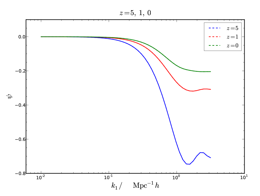
In Fig. 13, we show the evolution of the kernel $\psi$ and its components at $z=5$, 1 and 0 respectively. The parameters used are the same as those in the previous section and we have set $k_{1}=k_{2}$ and $\mu=-1/2$. Similar to the case of $b_{1}$, there is no noticeable difference between the case with static window and the evolving one. All these contributions peaks around $k\sim 0.7-0.9\,\mathrm{Mpc}^{-1}\,h$. In this case, $T_{\epsilon_{1}^{*}}$ and $T_{\epsilon_{\rm v}^{*}}$ are of similar magnitude but opposite signs, so they roughly cancel each other. Thus the net contribution is mainly given by $T_{J}$. The overall contribution of $\psi$ decays over time.

Again to highlight the effects of the initial scale-dependent bias, we show the case when the initial condition is scale-independent, i.e. $b_{1}^{*}=b_{\nu}$ and $b_{\rm v}^{*}=1$ are assumed in Fig. 14. We find that the bump around $k\sim 1\,\mathrm{Mpc}^{-1}\,h$ Fig. 13 is no longer present, instead there is smooth transition from $k\sim 0.2$ to $1\,\mathrm{Mpc}^{-1}\,h$.

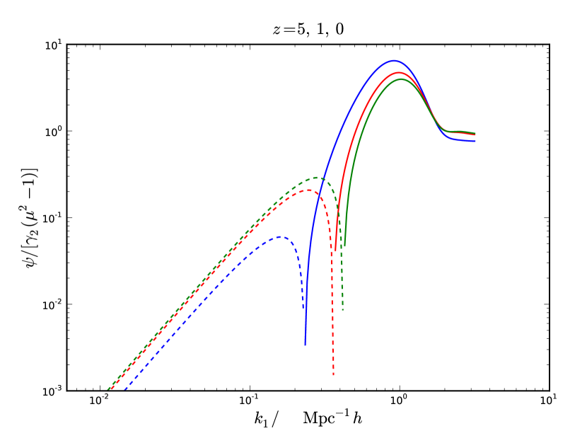
The second order kernel will contribtute to the tree level bispectrum. As a quick check of the importance of the correction term, we compare the kernel $\psi$ with the nonlocal term kernel $\gamma_{2}(\mu^{2}-1)$ in Fig. 15. The parameters used are the same as the previous ones. From Fig. 15, we can see the $k^{2}$ correction at low $k$. However, the $k^{2}$ correction term starts to surpass the nonlocal term at $k\sim 0.4\,\mathrm{Mpc}^{-1}\,h$. Hence one should also find the signature of the $k^{2}$ correction term in the halo bispectrum at $k\gtrsim 0.2\,\mathrm{Mpc}^{-1}\,h$.

Figure 12: The evolution of the kernel of $\theta_{\rm g}^{(2)}$ for the case with static window (dashed) and the SC evolving one (solid). The parameters $k_{1}=k_{2}$ and $\mu=-1/2$ are used. Three redshifts are shown, $z=5$ (blue), 1 (red) and 0 (green).

Figure 13: The evolution of the kernel of $\psi$ for the case with static window (dashed) and the SC evolving one (solid). However, these two cases are indistinguishable. The parameters are set such that $k_{1}=k_{2}$ and $\mu=-1/2$. Three redshifts are shown, $z=5$ (blue), 1 (red) and 0 (green).

Figure 14: Same as Fig. 13, except with scale-independent initial conditions $b_{1}^{*}=b_{\nu}$ and $b_{\rm v}^{*}=1$.

Figure 15: The ratio between the kernel $\psi$ and $\gamma_{2}(\mu^{2}-1)$, the kernel of the nonlocal term $\mathcal{G}_{2}$. The parameters $k_{1}=k_{2}$ and $\mu=-1/2$ are used. Three redshifts are shown, $z=5$ (blue), 1 (red) and 0 (green). Solid line for positive value and dotted line for negative one.

IV Conclusions

Recent measurements of the velocity bias suggest that the velocity bias of the halos is non-negligible at the weakly nonlinear regime $k\sim 0.1\,\mathrm{Mpc}^{-1}\,h$ at late time. In the time evolution model of the halo field, previously it was shown that it leads to decay of the initial velocity bias using the point particle approximation so that it becomes negligible at late time. On the other hand, the peak model gives constant velocity bias over time. Thus the measurement seems to be in favour of the peak model result.

It is often assumed that halos are point particles and focus only on their center of mass. Here we argue that as halos consist of a collection of particles, the force acting on its CM of the halo should be the force averaged over its constituent particles instead of only the force at the position of the CM. To take into account of the halo profile, we introduce a window function in the Euler equation. We find that the window function leads to non-negligible $k^{2}$ correction to the linear velocity bias. While the initial $k^{2}$ velocity bias decays away, the correction due to profile correction does not. In contrast, in the peak model, the imposition of the peak constraint leads to an extra constant scale-dependent bias. This difference can be used to distinguish these models. The profile correction also gives $k^{2}$ correction to the second order velocity kernel. For the density bias, the effect of the profile correction is not important at low $k$ because the magnitude of the initial scale-dependent density bias is large in the peak model. Thus even at low $z$, the magnitude of the terms due to $b_{1}^{*}$ are the most important ones. Nonetheless, this implies that the $k^{2}$ correction is non-negligible for $k\gtrsim 0.2\,\mathrm{Mpc}^{-1}\,h$, especially for bispecturm.

Since the window function is dynamical, we model it using the spherical collapse model. We also measure the evolution of the halo profile by constructing proto-halos at different redshifts. To our knowledge this is the first systematic numerical study of the evolution of the proto-halo profile. We find that the proto-halo profile evolves from a top-hat-like profile to an NFW profile. We find reasonable agreement between the spherical collapse and the numerical results. On the theory side, one may improve the modelling using ellipsoidal collapse model instead. Computationally, it would be useful to come up with a parameterization for the halo profile at various epochs.

Our work has highlighted the importance of halo profile and its evolution on bias. In theories such as the excursion set theory and peak model, window function are used to define halos in Lagrangian space. They are often assumed to be static and the window size given by the Lagrangian size even when they are transformed to the Eulerian space. The idea of profile evolution can be easily applied to these models as well.

In our model, the effect of the window function correction is most apparent in the velocity bias. Although there are some existing measurements of velocity bias, it is still hard because it is prone to sampling artifacts. We hope to report the comparison of our model with velocity bias measurement in future.

References

- Kaiser (1987) N. Kaiser, MNRAS 227, 1 (1987).
- Hamilton (1992) A. J. S. Hamilton, ApJ 385, L5 (1992).
- Song and Percival (2009) Y.-S. Song and W. J. Percival, JCAP 10, 4 (2009), arXiv:0807.0810 .
- Taruya et al. (2014) A. Taruya, K. Koyama, T. Hiramatsu, and A. Oka, Phys. Rev. D 89, 043509 (2014), arXiv:1309.6783 .
- Guzzo et al. (2008) L. Guzzo, M. Pierleoni, B. Meneux, E. Branchini, O. L. Fevre, C. Marinoni, et al., Nature 451, 541 (2008), arXiv:0802.1944 .
- Blake et al. (201) C. Blake, E. A. Kazin, F. Beutler, T. M. Davis, D. Parkinson, S. Brough, et al., MNRAS 418, 1707 (201), arXiv:1108.2635 .
- Reid et al. (2012) B. A. Reid, L. Samushia, M. White, W. J. Percival, M. Manera, N. Padmanabhan, et al., MNRAS 426, 2719 (2012).
- Beutler et al. (2012) F. Beutler, C. Blake, M. Colless, D. H. Jones, L. Staveley-Smith, G. B. Poole, et al., MNRAS 423, 3430 (2012).
- Samushia et al. (2013) L. Samushia, B. A. Reid, M. White, W. J. Percival, A. J. Cuesta, et al., MNRAS 429, 1514 (2013), arXiv:1206.5309 .
- de la Torre et al. (2013) S. de la Torre, L. Guzzo, J. A. Peacock, E. Branchini, A. Iovino, B. R. Granett, et al., A&A 557, A54 (2013), arXiv:1303.2622 .
- Oka et al. (2014) A. Oka, S. Saito, T. Nishimichi, A. Taruya, and K. Yamamoto, MNRAS 439, 2515 (2014), arXiv:1310.2820 .
- Koda et al. (2014) J. Koda, C. Blake, T. Davis, C. Magoulas, C. M. Springob, M. Scrimgeour, et al., MNRAS 445, 4267 (2014), arXiv:1312.1022 .
- Elia et al. (2002) A. Elia, A. D. Ludlow, and C. Porciani, MNRAS 421, 3472 (2002), arXiv:1111.4211 .
- Chan et al. (2012) K. C. Chan, R. Scoccimarro, and R. K. Sheth, Phys. Rev. D 85, 083509 (2012), arXiv:1201.3614 .
- Baldauf et al. (2014) T. Baldauf, V. Desjacques, and U. Seljak, (2014), arXiv:1405.5885 .
- Jennings et al. (2014) E. Jennings, C. Baugh, and D. Hatt, (2014), arXiv:1407.7296 .
- Zheng et al. (2014a) Y. Zheng, P. Zhang, and Y. Jing, (2014a), arXiv:1410.1256 .
- Scoccimarro (2004) R. Scoccimarro, Phys. Rev. D 70, 083007 (2004).
- Juszkiewicz et al. (1995) R. Juszkiewicz, D. H. Weinberg, P. Amsterdamski, M. Chodorowski, and F. Bouchet, ApJ 442, 39 (1995).
- Zhang et al. (2014) P. Zhang, Y. Zheng, and Y. Jing, (2014), arXiv:1405.7125 .
- Zheng et al. (2014b) Y. Zheng, P. Zhang, and Y. Jing, (2014b), arXiv:1409.6809 .
- Okumura et al. (2012) T. Okumura, U. Seljak, P. McDonald, and V. Desjacques, JCAP 02, 010 (2012), arXiv:1109.1609 .
- Elia et al. (2011) A. Elia, S. Kulkarni, C. Porciani, M. Pietroni, and S. Matarrese, MNRAS 416, 1703 (2011), arXiv:1012.4833 .
- Desjacques et al. (2010) V. Desjacques, M. Crocce, R. Scoccimarro, and R. K. Sheth, Phys. Rev. D 82, 103529 (2010), arXiv:1009.3449 .
- Biagetti et al. (2014a) M. Biagetti, V. Desjacques, A. Kehagias, and A. Riotto, Phys. Rev. D 90, 103529 (2014a), arXiv:1408.0293 .
- Desjacques and Sheth (2010) V. Desjacques and R. K. Sheth, Phys. Rev. D 81, 023526 (2010), arXiv:0909.4544 .
- Seljak (2000) U. Seljak, MNRAS 318, 203 (2000).
- Peacock and Smith (2000) J. A. Peacock and R. R. Smith, MNRAS 318, 1144 (2000).
- Scoccimarro et al. (2001) R. Scoccimarro, R. K. Sheth, L. Hui, and B. Jain, ApJ 546, 20 (2001).
- Cooray and Sheth (2002) A. Cooray and R. Sheth, Phys. Rep. 372, 1 (2002), arXiv:astro-ph/0206508 .
- Navarro et al. (1996) J. F. Navarro, C. S. Frenk, and S. D. M. White, ApJ 462, 563 (1996).
- Gunn and Gott (1972) J. E. Gunn and J. R. Gott, III, ApJ 176, 1 (1972).
- Peebles (1980) P. J. E. Peebles, The Large-Scale Structure of the Universe (Princeton University Press, New Jersey, 1980).
- Padmanabhan (1993) T. Padmanabhan, Structure formation in the Universe (Cambridge University Press, Cambridge, 1993).
- Mo et al. (2010) H. Mo, F. van den Bosch, and S. White, Galaxy Formation and Evolution (Cambridge University Press, Cambridge, 2010).
- Lynden-Bell (1967) D. Lynden-Bell, MNRAS 136, 101 (1967).
- Bindoni and Secco (2008) D. Bindoni and L. Secco, New Astronomy Reviews 52, 1 (2008).
- Bryan and Norman (1998) G. L. Bryan and M. L. Norman, ApJ 495, 80 (1998).
- Scoccimarro (1998) R. Scoccimarro, MNRAS 299, 1097 (1998), arXiv:astro-ph/9711187 .
- Crocce et al. (2006) M. Crocce, S. Pueblas, and R. Scoccimarro, MNRAS 373, 369 (2006), arXiv:astro-ph/0606505 .
- Eke et al. (1996) V. R. Eke, S. Cole, and C. S. Frenk, MNRAS 282, 263 (1996).
- Seljak and Zaldarriaga (1996) U. Seljak and M. Zaldarriaga, ApJ 469, 437 (1996), arXiv:astro-ph/9603033 .
- Springel (2005) V. Springel, MNRAS 364, 1105 (2005), arXiv:astro-ph/0505010 .
- Neto et al. (2007) A. F. Neto, L. Gao, P. Bett, S. Cole, J. F. Navarro, et al., MNRAS 381, 1450 (2007).
- Chan et al. (2015) K. C. Chan, R. K. Sheth, and R. Scoccimarro, in preparation (2015).
- Engineer et al. (2000) S. Engineer, N. Kanekar, and T. Padmanabhan, MNRAS 314, 279 (2000), arXiv:astro-ph/9812452 .
- Bond and Myers (1996) J. R. Bond and S. T. Myers, ApJS 103, 1 (1996).
- Shen et al. (2006) J. Shen, T. Abel, H. J. Mo, and R. K. Sheth, ApJ 645, 783 (2006).
- Sheth et al. (2001) R. K. Sheth, H. J. Mo, and G. Tormen, MNRAS 323, 1 (2001).
- Robertson et al. (2009) B. E. Robertson, A. V. Kravtsov, J. Tinker, and A. R. Zentner, ApJ 696, 636 (2009).
- Fry (1996) J. N. Fry, ApJL 461, L65 (1996).
- Baldauf et al. (2012) T. Baldauf, U. Seljak, V. Desjacques, and P. McDonald, Phys. Rev. D 86, 083540 (2012), arXiv:1201.4827 .
- Saito et al. (2014) S. Saito, T. Baldauf, Z. Vlah, U. Seljak, T. Okumura, and P. McDonald, Phys. Rev. D 90, 123522 (2014), arXiv:1405.1447 .
- Biagetti et al. (2014b) M. Biagetti, V. Desjacques, A. Kehagias, and A. Riotto, Phys. Rev. D 90, 045022 (2014b), arXiv:1405.1435 .
- Bel et al. (2015) J. Bel, K. Hoffmann, and E. Gaztanaga, (2015), arXiv:1504.02074 .
- Bernardeau et al. (2002) F. Bernardeau, S. Colombi, E. Gaztañaga, and R. Scoccimarro, Phys. Rep. 367, 1 (2002), arXiv:astro-ph/0112551 .
- Somogyi and Smith (2010) G. Somogyi and R. E. Smith, Phys. Rev. D 81, 023524 (2010), arXiv:0910.5220 .
- Bernardeau et al. (2012) F. Bernardeau, N. V. de Rijt, and F. Vernizzi, Phys. Rev. D 85, 063509 (2012), arXiv:1109.3400 .
- Scoccimarro et al. (1998) R. Scoccimarro, S. Colombi, J. N. Fry, J. A. Frieman, E. Hivon, and A. Melott, ApJ 496, 586 (1998), arXiv:astro-ph/9704075 .