Fluctuations and correlations in high temperature QCD
Abstract
We calculate second- and fourth-order cumulants of conserved charges in a temperature range stretching from the QCD transition region towards the realm of (resummed) perturbation theory. We perform lattice simulations with staggered quarks; the continuum extrapolation is based on in the crossover-region and at higher temperatures. We find that the Hadron Resonance Gas model predictions describe the lattice data rather well in the confined phase. At high temperatures (above 250 MeV) we find agreement with the three-loop Hard Thermal Loop results.
pacs:
12.38.Gc,12.38.Mh,11.10.WxI Introduction
The Quark Gluon Plasma was formed in the Early Universe just a few microseconds after the Big Bang; today it is produced in heavy ion collision experiments at the Large Hadron Collider (LHC) at CERN and the Relativistic Heavy Ion Collider (RHIC) at Brookhaven Lab (BNL). This phase exists at high temperatures and/or densities, and is separated from the hadronic phase of Quantum Chromodynamics (QCD) by a cross-over transition Aoki et al. (2006a). Lattice QCD has determined the temperature of this cross-over in Refs. Aoki et al. (2006b, 2009); Borsanyi et al. (2010a); Bazavov et al. (2012a).
Below the transition temperature, the thermodynamics is governed by massive hadrons with integer charges, whereas at high temperature nearly free and nearly massless quarks with fractional charges and gluons dominate. Fluctuations of various conserved charges are sensitive probes of the quantum numbers and the associated masses, and have been proposed as a signal of the deconfinement transition Jeon and Koch (2000); Asakawa et al. (2000). In heavy ion experiments there is an ongoing effort to measure the moments of conserved charge distributions Luo (2015), which can be related one-to-one to fluctuations. They are particularly interesting for the beam energy scan program at RHIC, since they may signal a nearby critical end point: higher order moments of net proton distributions are sensitive to an increase in the correlation length Stephanov et al. (1999). Fluctuations can also be used to extract the chemical freeze-out temperature and chemical potential Karsch and Redlich (2011), as an alternative method to the thermal fits to particle yields or ratios Becattini et al. (2006); Cleymans et al. (2006); Andronic et al. (2006, 2009); Becattini et al. (2014). The STAR collaboration has published the first four moments of the net-proton Adamczyk et al. (2014a) and net-electric charge Adamczyk et al. (2014b) distributions. In parallel to the experimental efforts, the past years have witnessed a rapid development in the lattice calculations of fluctuations Bazavov et al. (2012b); Borsanyi et al. (2013a), leading to quantitative estimates of the chemical freeze-out temperature and chemical potential for a range of RHIC energies Borsanyi et al. (2014a).
Diagonal quark number susceptibilities have already been calculated in the early dynamical simulations Gottlieb et al. (1987, 1988); Gavai et al. (1989); these were later complemented by the off-diagonal ones Gavai et al. (2002); Gavai and Gupta (2003); Allton et al. (2002); Bernard et al. (2005); Gavai and Gupta (2006); Allton et al. (2005). In the following years, higher order fluctuations have been calculated up to the sixth order Allton et al. (2005); Datta et al. (2013), with the main motivation to extrapolate several thermodynamic observables to larger values of the chemical potential. These were staggered simulations projects, but studies with Wilson quarks are also emerging Borsanyi et al. (2012a, 2015a); Giudice et al. (2014); Aarts et al. (2015); Gattringer and Schadler (2015). Strangeness fluctuations were used also to locate the transition temperature and, for this purpose, they were continuum extrapolated. With Wilson quarks this was done with pion masses down to 285 MeV Borsanyi et al. (2012a, 2015a), for staggered quarks the continuum limit was calculated at the physical point Aoki et al. (2006b, 2009); Borsanyi et al. (2010a); Bazavov et al. (2012c). Continuum results for the other second cumulants appeared first in Ref. Borsanyi et al. (2012b) then in Ref. Bazavov et al. (2012c). Selected higher order fluctuations were continuum extrapolated first in Refs. Borsanyi (2013); Borsanyi et al. (2013a); Bellwied et al. (2013); Bazavov et al. (2013a).
Below the cross-over temperature, hadrons (mesons and baryons) dominate the thermodynamics. In this regime, the Hadron Resonance Gas (HRG) model provides a simple description of thermodynamic quantities, including specific fluctuations or correlations Dashen et al. (1969); Venugopalan and Prakash (1992). Even before simulations with physical quark masses could be performed, lattice QCD data were well described by the HRG model if the actual particle spectrum was replaced by the unphysical one simulated on the lattice Karsch et al. (2003); Huovinen and Petreczky (2010). The success of the HRG model based on the experimental resonance table has been demonstrated later in several papers with physical quark masses and continuum extrapolation for the chiral condensate Borsanyi et al. (2010a), the equation of state Borsanyi et al. (2014b) and fluctuations Borsanyi et al. (2012b); Bazavov et al. (2012c).
The concept of HRG has motivated new studies where fluctuation-based observables were proposed for which, within the framework of the HRG model, only particles and resonances with a specific quantum number contribute (e.g. baryons in a specific strangeness sector) Bazavov et al. (2013b). Since at low most lattice results agree with the HRG predictions, which is no longer true in the deconfined phase, the highest temperature of agreement can be a model-dependent indicator of deconfinement, that can be studied on a flavor-specific basis Bellwied et al. (2013).
Very high temperature QCD is best discussed in terms of improved perturbation theory. The QCD thermodynamic potential is known up to order Kajantie et al. (2003). This result was later generalized to finite chemical potentials Vuorinen (2003a) and the quark number susceptibilities were calculated to the same order Vuorinen (2003b). The soft contributions to these unimproved perturbative results can be resummed via dimensional reduction Blaizot et al. (2003a). This idea has been applied to the four-loop perturbative quark number susceptibilities Andersen et al. (2013); Mogliacci et al. (2013).
The hard thermal loop perturbation theory reorganizes the perturbative series, enhancing its convergence Braaten and Pisarski (1992); Andersen et al. (2002). Recently, the next-to-next-to-leading order pressure and energy density were calculated for the SU(3) theory, Andersen et al. (2010), dramatically improving the agreement with lattice simulations Boyd et al. (1996); Borsanyi et al. (2012c). Soon afterwards, the full QCD result was calculated, too Strickland et al. (2011); Andersen et al. (2011). Fluctuations were calculated at one Andersen et al. (2013), two Haque et al. (2013) and three loop order Haque et al. (2014a), improving the earlier HTL calculations of susceptibilities Blaizot et al. (2001, 2003b). This result was later generalized to finite chemical potentials Haque et al. (2014b).
In general, these highly resummed perturbative results are expected to provide a good approximation, but their range of validity can only be determined if they are compared with a non-perturbative approach, e.g. lattice QCD simulations. Such comparisons have already been made, first on the level of the equation of state Andersen et al. (2011). Unfortunately, for this observable, the renormalization scale-dependence is too large for a definitive answer on the range of validity. Fluctuations, however, offer a more strict test for these diagrammatic approaches because of the rather small renormalization scale dependence of the result from dimensional reduction (DR) Mogliacci et al. (2013) and from hard thermal loops (HTL) Haque et al. (2014a). Today lattice calculations at high temperatures are available e.g. with the HISQ action of the BNL-Bielefeld group Bazavov et al. (2012c, 2013a) and also with the 2stout action of the Wuppertal-Budapest collaboration Borsanyi et al. (2012b); Borsanyi (2013).
In this paper, we present results on diagonal and non-diagonal second and fourth order fluctuations, in a temperature range which stretches from the transition region to the perturbation theory domain. Our simulations are performed within the 2nd generation staggered thermodynamics program (4stout action). We start with the discussion of the conserved charges in the grand canonical field theory and provide details on how their fluctuations are calculated on the lattice. After describing our lattice thermodynamics program, the scale setting procedure and the finite temperature simulations, we highlight the technical challenges of a continuum extrapolation and the estimate of the systematic error on the continuum results. The results are organized in two sections. First we consider the cross-over region, around the point where the Hadron Resonance Gas loses its predictive power. Afterwards we compare our data to (resummed) perturbative results at high temperatures. We close with some concluding remarks pointing to further directions of research.
II Fluctuations in lattice QCD
II.1 QCD as a grand canonical ensemble
In a canonical ensemble, the conserved charges are external parameters. In a heavy ion collision, for example, the number of baryons, their electric charge and the vanishing strangeness are fixed during the entire collision, expansion of the plasma and freeze-out. A grand canonical ensemble emerges if a small sub-system is considered, that is still large enough to be close to the thermodynamic limit Bzdak et al. (2013).
In QCD there exists a conserved charge for each quark flavor, thus one can introduce four quark chemical potentials in a flavor system: , , and , in short .
The expectation number of a conserved charge is then found as a derivative with respect to the chemical potential.
| (1) |
The response of the system to the thermodynamic force is proportional to the fluctuation of the conserved charge:
| (2) |
Since is an extensive thermodynamic quantity and so is its -derivative, there the contributions cancel in Eq. (2). Charge conjugation symmetry implies that, at , the expectation value of any odd combination vanishes, e.g. the last term in Eq. (2). However, there is no such symmetry for different flavors, allowing e.g. for a correlator. The first perturbative diagram that contributes to the latter consists of two fermion loops, connected by three gluon lines Blaizot et al. (2001).
The free energy density () is proportional to the pressure in large volumes:
| (3) |
The derivatives with respect to the chemical potential can thus be written in terms of the pressure:
| (4) |
with . This normalization ensures that the cumulants stay dimensionless, and become finite in the infinite volume and infinite temperature limit. In this normalization is the expected number of quarks of the given flavor in a volume .
The higher derivatives with respect to the same quark chemical potential correspond to the higher moments of that flavor:
| (5) |
In experiment, the net-charge distribution moments are measured, each carrying an unknown volume factor. A known caveat is the fluctuation of these volumes themselves. The study of these goes beyond the scope of this paper, see Skokov et al. (2013); Alba et al. (2015). For a fixed volume, though, the volume factor can be simply cancelled out by forming ratios of cumulants of the same conserved charge:
| ; | |||||
| ; | (6) |
Phenomenological models and experiments usually work in the baryon number () - electric charge () - strangeness () basis. Since the charm quark plays a negligible role in the transition region one can express these directions in the space as a three-dimensional transformation:
| (7) | |||||
| (8) | |||||
| (9) |
The fluctuations of the conserved charges (, and ) can then be expressed in terms of the quark derivatives. In addition, the ( component of the) light isospin is often studied with . Assuming zero chemical potential and degenerate and quarks on the lattice, several simplifications occur, and we have Bernard et al. (2005); Bazavov et al. (2012c):
| (10) | |||||
| (11) | |||||
| (12) | |||||
| (13) | |||||
| (14) | |||||
| (15) |
Indeed, due to the degeneracy the six second order combinations in the , , space can be expressed in terms of four quark correlators. There are 15 fourth order correlators in the () space that can be expressed in terms of 9 fourth order quark-correlators. The kurtosis of the baryon and the electric charge is given by the following correlators:
| (16) | |||||
| (17) |
other, mixed derivatives can be calculated analogously.
At high temperature, fluctuations approach the Stefan-Boltzmann limit. For an ideal gas, the pressure at finite chemical potential reads Kapusta and Gale (2006); Toimela (1983)
| (18) |
For the second and fourth order fluctuations this means that in the high temperature limit and , and no mixed derivatives survive.
II.2 Fluctuations on the lattice
The standard way to introduce the chemical potential on the lattice is to modify the temporal links, like the component of a homogeneous U(1) field Hasenfratz and Karsch (1983):
| (19) |
The fermion matrix is built from the -dependent links. In the staggered formalism, which we will use in this paper, each fermion flavor may carry an independent chemical potential. The fermion determinants express a single quark flavor.
| (20) |
where is the gauge action. To be specific, in this paper we use the tree-level Symanzik improvement in , however its form plays no role in the fluctuation-related formulas. The derivative of the staggered fermion matrix takes the following from:
any higher odd derivative is equal to , while any higher even derivative is equal to . is the Kogut-Susskind phase factor.
For the fourth order -derivative one has to evaluate the fourth derivatives of . These are traces of the fermion matrix that have to be calculated for every generated finite temperature configuration Allton et al. (2002):
| (21) | |||||
| (22) | |||||
| (23) | |||||
| (24) | |||||
Using the simple notation for , the derivatives can now be written for the full free energy:
| (25) |
The derivative of the expectation value of any lattice observable is obtained as
| (26) |
When we derive the higher order formulas (see also Allton et al. (2002)) we assume non-zero chemical potential and use Eq. 26 recursively. Setting in the end we have, to second order,
| (27) |
and to fourth order, exploiting the degeneracy between the light quark flavors:
| (28) | |||||
| (29) | |||||
| (30) | |||||
| (31) | |||||
| (32) | |||||
| (33) | |||||
| (34) | |||||
| (35) | |||||
We follow the standard stochastic strategy to calculate the traces , and evaluate them with a large number of Gaussian random sources. If one is only interested in up to the fourth derivative, five calls to the linear solver are necessary for each random source. Since the operator appears only in connected contributions, we do not need it to high accuracy. , on the other hand, appears in the disconnected term with the most difficult cancellation, so it needs to be evaluated more often. requires one solver, while requires three solvers. Thus, if we evaluate with sources, we evaluate the operator times and the and operators times.
It was pointed out in Allton et al. (2002) that, when products of traces are calculated (e.g. ), the two (or more) operators in the product must be calculated with different (or uncorrelated) random sources. For this reason, we always use quartets of independent sources. We typically use quartets in our analysis. Multi-right-hand-side solvers are particularly useful in this context, since these typically achieve a higher flop rate on many supercomputers, because the gauge fields do not have to be loaded from the memory with each source Kaczmarek et al. (2014).
The numerical evaluation of these diagrams with multiple random sources can be accelerated by various means. One observation was that e.g. the operator can be split into two parts , where is the result of a truncated solver and is the difference between the truncated result and the full precision solution. The advantage is that can be evaluated with less sources, while the more noisy is cheaper to work with Bali et al. (2010).
III Lattice action and ensembles
This work is part of the second generation thermodynamics program of the Wuppertal-Budapest collaboration. We use the tree-level Symanzik gauge action with 2+1+1 flavors of four times stout smeared staggered quarks Morningstar and Peardon (2004), with the smearing parameter .
III.1 Zero temperature simulations and the line of constant physics
An essential step, before thermodynamics runs can be started with a new action, is the tuning of the mass parameters and the determination of the scale or, in other words, the mass and coupling renormalization of the theory for each lattice cut-off that the thermodynamics project intends to use. In this project we use degenerate up and down quarks. For simplicity, we do not tune the charm mass separately but accept the continuum extrapolated quark mass ratio of Ref. Davies et al. (2010). The light and strange quark masses are obtained by tuning the following ratios to their physical values:
| (36) |
where we use the isospin-averaged pion and kaon masses ( and ) Aoki et al. (2014). (see Ref. Rosner and Stone (2013)) is used to set the scale.
In this work we use the zero temperature lattice configurations produced for the 4stout project Borsanyi et al. (2015b). In the lattice spacing range we simulate four or more ensembles for eight inverse bare couplings . The RHMC streams for the ensembles are typically trajectories long after thermalization. We parametrized these ensembles such that they form a bracket around the physical point, which is defined in Eq. (36). The box size of these zero temperature simulations was without exception .
In Fig. 1 we summarize the zero temperature configurations. For each we interpolated in the space of bare quark masses, getting these to a few per mill accuracy. On the left panel of Fig. 1 we show the combinations in Eq. (36). The right panel shows the position of individual bare parameters relative to the thus interpolated physical point (with details given in Ref. Borsanyi et al. (2015b)).
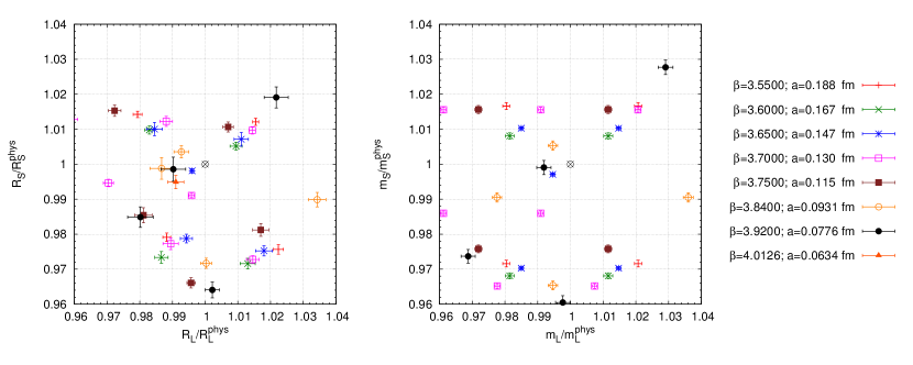
Our finest large volume ensemble was simulated at on a lattice. Its parameters were extrapolated and then corrected using simulations at this in the flavor symmetric point, where all three light quark masses are degenerate (the charm mass staying physical).
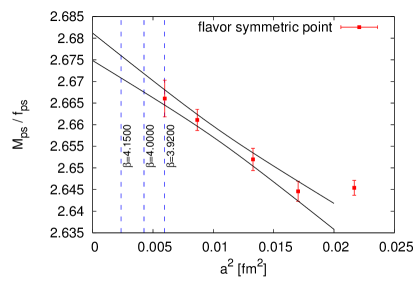
The tuning effort using the flavor symmetric lattices goes as follows: first, we have to acknowledge that various scale setting schemes differ in the cut-off effects. Thus, changing the scale setting or tuning principle may introduce different cut-off effects on different parts of the line of constant physics. A continuum extrapolation that spans a larger range of lattice spacings will thus be distorted. To prevent this from happening, we match not only the scale but also the corrections and check for the insignificance of the effects whenever we are forced to switch between scale setting schemes along the line of constant physics. In this particular case, we chose the mass-independent renormalization scheme. For a fixed gauge coupling, we define a 3+1 flavor theory with the bare masses calculated from the ones of the 2+1+1 flavor theory: , . This corresponds to a new scheme, and the pseudo-scalar mass to decay constant ratio will have an dependence. We plot this ratio in Fig. 2 (notice that, in the 2+1+1 theory, had no -dependence by definition). To extract the bare quark masses of the 2+1+1 dimensional theory at and , we performed several simulations in the 3+1 flavor theory and interpolated in to match the extrapolation in Fig. 2. We translated the masses back to the 2+1+1 flavor theory. At this point, we had to assume the ratio, (which is consistent to our estimate from this work) Davies et al. (2010); McNeile et al. (2010); Durr et al. (2011a, b). For the large volume simulation at , which was running with such an indirectly tuned mass, we show the result in Fig. 1: the physical point is reproduced with an accuracy below one percent. The lattice spacings are shown in the plot, for the finest lattice we used the SU(2) low energy constants to extrapolate the final one percent to the physical point Borsanyi et al. (2013b).
For even finer lattices we had to resort to a perturbative continuation of the line of constant physics. For the scale setting, the universal two-loop beta function does not yet describe the data. We have an alternative scale setting scheme , introduced in Borsanyi et al. (2012d), which is based on the gradient flow Luscher (2010). In that case, finite volume effects are small even for lattices as small as fm Borsanyi et al. (2012d). This allowed to match again the value and -dependence of at ( fm) and ( fm). The exploding autocorrelation times have forced us to use extremely long update streams (cca. 50000 trajectories) in a volume. For even finer lattices we again measured and matched the flow and its leading lattice artefacts in fixed physical volume and topological sector in several subsequent steps. The final scale is plotted in Fig. 3. Since is of great interest for a wider community we will discuss its value, volume-dependence and other systematics in a publication devoted solely to scale setting.
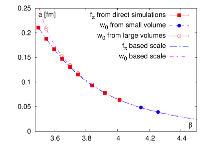
Fig. 3 shows two versions of the scale setting. Controlled continuum extrapolations are independent of the choice of the scale setting scheme. The equivalence of the schemes on fine lattices is evident from Fig. 3. Nevertheless, this choice obviously influences the temperature of a particular ensemble. Especially for observables with large slope in temperature (e.g. the quark number susceptibilities in the cross-over region) the scale setting has an impact on the continuum scaling. We propagate this effect into the final error bars by calculating the continuum limits with both scale settings and include this in our study of systematics.
III.2 Finite temperature ensembles
We have generated three sets of ensembles, each with multiple lattice spacings and temperatures. In the first set we use the aspect ratio , which might have finite volume effects, but gives a more favorable signal/noise ratio than larger volumes. The second set has and covers the entire transition range up to . Using these ensembles we can conclude that, wherever it was possible to perform a meaningful comparison (this includes all second order fluctuations and cross-correlators), finite volume effects on the ensembles are negligible for any lattice spacing, let alone in the continuum limit which is the largest source of systematic errors. We see significant finite volume effects only in the chiral condensate and susceptibility, which are not part of this study. For temperatures MeV we do not keep the lattice geometry constant in our temperature scan, but keep the physical volume more-or-less constant with . For the finest, lattices in this set we have thus used the lattices , , and for and 600 MeV, respectively. In the high temperature range, the statistics is limited to 1000 configuration / temperature / lattice spacing.
Table 1 shows the statistics for the ensembles in the cross-over region and in the quark gluon plasma phase. The temperatures below 150 MeV are used to compare the data to the predictions of the Hadron Resonance Gas model. The data set is restricted to the cross-over region (see table 2). In the tables we give the number of configurations that we have analyzed for generalized quark number susceptibilities: these are separated by ten Rational Hybrid Monte Carlo (RHMC) trajectories. The acceptance range varies between 80 and 95%.
In the absence of visible finite volume effects in this range, we combine the results of these with the data set to enhance the signal. Indeed, the fluctuations of disconnected diagrams (especially ) in Eq. (28) are heavily penalized by large volumes. This contribution also appears in the Taylor coefficients of the expansion and is the main source of noise.
| [MeV] | |||||
| 125 | 10514 | 10080 | 10008 | 5027 | 2060 |
| 130 | 5766 | 4625 | 10253 | 5099 | 2000 |
| 135 | 14762 | 10590 | 10060 | 10189 | 2720 |
| 140 | 14863 | 5381 | 15043 | 4959 | 5097 |
| 145 | 5784 | 5020 | 10014 | 5019 | 1280 |
| 150 | 5464 | 5067 | 11043 | 5064 | 1631 |
| 153 | 4985 | 5517 | 6410 | 3641 | - |
| 155 | 5613 | 5001 | 10137 | 5015 | 1726 |
| 157 | 5526 | 5409 | 10018 | 5160 | 1065 |
| 160 | 5247 | 5017 | 4973 | 5073 | 1082 |
| 165 | 8169 | 10086 | 10496 | 5000 | 1000 |
| 170 | 6005 | 6113 | 5600 | 5111 | 600 |
| 175 | 12018 | 5375 | 5058 | 5104 | 972 |
| 180 | 5007 | 5089 | 5034 | 5013 | 1000 |
| 190 | 4900 | 5031 | 5121 | 5045 | 992 |
| 200 | 5989 | 5002 | 6722 | 1012 | 1000 |
| 220 | 5514 | 5000 | 7231 | 1003 | 1000 |
| 240 | 1712 | 5000 | 8082 | 3947 | 1000 |
| 250 | 10695 | 5685 | 5146 | - | - |
| 260 | 6287 | 5000 | 8623 | 5441 | 1000 |
| 270 | 11574 | 5682 | 5684 | - | - |
| 280 | 7067 | 5003 | 8751 | 1021 | 558 |
| 290 | 7316 | 5680 | 5684 | - | - |
| 300 | 5125 | 4917 | 5398 | 5310 | 1011 |
| [MeV] | |||||
|---|---|---|---|---|---|
| 130 | 39161 | 7736 | 10351 | - | 2007 |
| 135 | 41462 | 8724 | 10696 | 9892 | 3000 |
| 140 | 39867 | 8550 | 10240 | 8248 | 1551 |
| 145 | 40247 | 8518 | 10348 | 10130 | 2550 |
| 150 | 39996 | 8461 | 10569 | 6717 | 3044 |
| 155 | 19953 | 8625 | 10345 | 10211 | 1546 |
| 160 | 20015 | 9174 | 11611 | 10140 | 2063 |
| 165 | 10965 | 9750 | 10219 | 10136 | 1200 |
III.3 Continuum extrapolation
The continuum extrapolation is mostly based on all available lattice spacings. Since fine lattices have lower statistics, the coarsest results are usually included only in non-linear extrapolations, (e.g. and other variations, where is the continuum limit).
While for some observables (e.g. , ) there is a clear range of safe linear extrapolation (in most cases ), observables that are related to pion physics (e.g. , ) show a very strong, non-linear dependence. Only for very fine lattices () we see a linear regime. Such behaviour have been already reported for the second order cumulants Borsanyi et al. (2012b); Bazavov et al. (2012c).
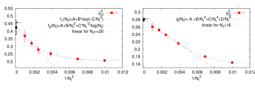
Here we show the charge fourth and second moment for a single temperature in the confined phase ( MeV) in Fig. 4. This plot features an additional point with 1485 analyzed configurations. We attempt several fit models, resembles a Boltzmann factor with an artefact mass vanishing as . is similar to including a term into the extrapolation. The shown continuum limit is based on the linear fit only.
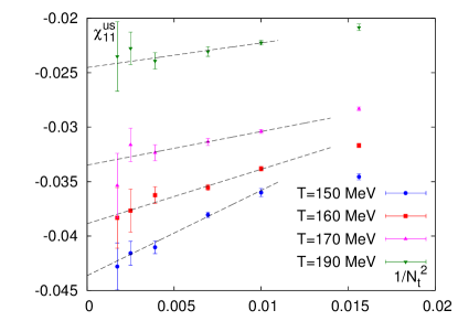
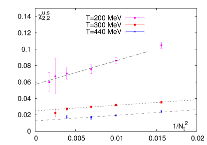
Not all observables require the finest lattices in our data set. Strange quark correlators receive no pion contributions, and the small relative taste violation in the kaon sector can be extrapolated away. We find that our data with its current precision allow linear fitting for . As examples we show the up-strange correlator () and the higher order correlator between the same quarks in Fig. 5. Both have only disconnected contributions (see Eqs. (27,31)).
The parameters of the finite temperature runs have been tuned to have the same temperature in the scale setting scheme. Since we also use the scale setting scheme, in that case the temperatures are no longer aligned and interpolations are necessary. The alignment of the temperatures is also not perfect in the scale setting scheme, thus we interpolate all data sets. The interpolation is performed by fitting a spline through several (7-9) node points with two different sets of nodes so that the systematics of the interpolation can be picked up by the systematic error. We then perform the continuum extrapolation temperature by temperature, for those temperatures for which we had data points. The lattice artefacts of the diagonal fluctuations can be understood from tree-level perturbative diagrams Gavai and Gupta (2003). We can correct for the -independent part of the discretization errors by a -independent factor (tree level improvement) Borsanyi et al. (2010b). This factor converges to 1 in the continuum limit. We perform the continuum extrapolation in three possible ways: without this improvement, with the tree-level improvement, and with the improvement factor of the free energy, that we find empirically to also reduce the cut-off effects at intermediate temperatures. We must then judge for every observable separately whether we can include the and ensembles, and which non-linear models are plausible and match the data. We have given examples for this in Fig. 4, but very often we simply add the models and to the linear fit.
We treat every mentioned option independently and perform 16–32 analyses per temperature, depending on the complexity of the continuum scaling. We use this large set of analyses to estimate the systematic errors temperature by temperature using the histogram method introduced in Refs. Durr et al. (2008); Borsanyi et al. (2015c). In this paper we build a histogram of the results. The analyses with a fixed data set but different systematics are weighted using the Akaike Information Criterion (AIC) Akaike (1974). The AIC weigted results corresponding to the various fit windows in are combined with uniform weights. In the case of the charm susceptibility we calculate the systematic errors on the finite points first and then perform various continuum extrapolations which then enter the histogram method. Since all analyses are equally we identify the median with the result. The distribution of results is not necessarily Gaussian and may contain isolated combinations of the analysis options that produce outliers. These do not contribute to the median. The systematic error is the spread of the distribution. Instead of the standard deviation we use the spread of central 68% of the distribution, so that we do not have to make assumptions on the tail of the distribution. The median can be calculated for every jackknife or bootstrap sample. We use the variance of the median as statistical error. In the plots we show the combined errors, by adding up the systematic and statistical errors in quadrature.
IV Results in the cross-over region
Previous works have suggested that the Hadron Resonance Gas (HRG) model provides a good description of the data in the range 130-150 MeV Huovinen and Petreczky (2010); Borsanyi et al. (2014b, 2010a, 2012b); Bazavov et al. (2012c), and perhaps missing strange resonances might account for the small deviations in the strangeness sector Bazavov et al. (2014a).
In this paper we supplement the picture with additional continuum extrapolated data. Finite lattice spacing studies (with or without a well improved action) can never state with certainty whether deviations from the model are a genuine effect. Here we compare our lattice results using the 2014 edition of the Particle Data Book Olive et al. (2014).
In our previous paper Borsanyi et al. (2012b) we have calculated nearly all the second order fluctuations. Only the most difficult correlator was omitted , which is not only noisy but had severe lattice spacing effects, similar to in Fig. 4.
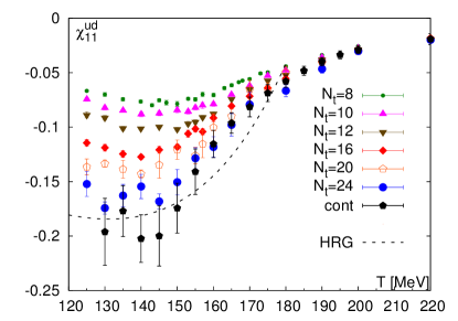
The continuum extrapolation of and the data in the full lattice spacing range are shown in Fig. 6, together with the up-strange correlator . The continuum limit for is well described by the HRG model up to MeV, which lies at the centre of the transition region Borsanyi et al. (2010a); Bazavov et al. (2012a). The main hadrons that contribute to the HRG prediction are the light mesons, mostly pions (the combination of a quark with an anti-quark makes the contribution negative). At high temperatures, heavier hadrons and their resonances have non-negligible Boltzmann factors, allowing the baryons (mostly protons) to take over the main role and bend the curve upwards.
The important role played by the pions is also highlighted by the staggered lattice artefacts (taste breaking) that increase the mass of the various staggered pion-like degrees of freedom (tastes) Bernard et al. (2006).
In lattice QCD in Eq. (27)’s notation. The operator is a trace over the whole lattice. The normalized Gaussian random sources () that we use to evaluate , contribute each as . This -odd estimator is widely oscillating between sources. Thus, in and then also in the stochastic representation of , large cancellations occur between opposite-sign contributions. Refs. Allton et al. (2002); Ejiri (2008) link the phase of the fermion determinant at small to the odd operators and . Indeed, the sign problem is already present in the Taylor-expansion technique and in the calculation of baryonic fluctuations in general.
The consequence is that the severity of the sign problem is related to the magnitude of . In early staggered studies one saw peak heights of Allton et al. (2002), Allton et al. (2005), and Bernard et al. (2005), are well short of today’s continuum limit in Fig. 6. With the early actions and coarse lattices the calculation of higher derivatives and reweighting were easier.
Note that the light isospin susceptibility () does not depend on the operator, , it does not contain any disconnected diagrams at all. The fourth derivative , too, contains only -even operators. Indeed, thermodynamics at finite isospin chemical potential is not plagued by the sign problem.
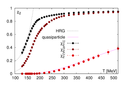
A subset of the authors of this paper have remarked that one can observe a hierarchy between flavors in their fluctuations Bellwied et al. (2013). We are now extending the picture and show the continuum extrapolations of the flavor-specific quark number susceptibilities in Fig. 7. The HRG model describes the light flavors reasonably well. The charm susceptibility in Fig. 7 rises at higher temperatures, compared to the lighter flavors. It was emphasized in Ref. Bazavov et al. (2014b) that open charm with fractional baryon charge starts appearing near the chiral crossover temperature. In addition to the hadron resonance gas model we show a naive quasiparticle estimate for the charm susceptibility (see also Petreczky et al. (2009)). The mass of the charm quark was fitted to the last points (). This mass is empirical, and may depend on the range of the matching to our lattice data. In general the mass of the charm quark is scheme dependent. The susceptibility curve runs near the quasiparticle model, qualitatively confirming that is contributed to by the deconfined charm quark. Nevertheless, the quasiparticle model’s results are overestimating the lattice data below approx. 350 MeV. This leaves room for multiple interpretations (e.g. -dependent , limitations of the quasiparticle model or charmonium bound states that absorb some of the free quarks).
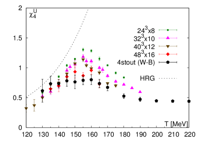
Figures 8 and 9 detail our continuum results for the fourth order cumulants. The normalized strangeness Bellwied et al. (2013) and baryon cumulants Borsanyi et al. (2013a); Bazavov et al. (2013b) have been published in earlier works. Here we show the fourth derivative with respect to the light single quark chemical potential (Fig. 8). On coarse lattices we see a strong peak around the transition temperature.
Such a peak has indeed been expected: if QCD is in the chiral scaling regime with an O() symmetry (i.e. the light quark masses are small enough for QCD being nearly chiral) then this scaling is expected to dominate the so called magnetic equation of state Ejiri et al. (2009), which parametrizes the singular part of the free energy as a reduced temperature and the quark masses that play the role of the magnetic field in the O() model’s language. The chemical potential enters through its shifting effect on the transition temperature. At finite , the reduced temperature is , where is the curvature of the QCD transition line Kaczmarek et al. (2011). Using the critical exponents one has, for the -th derivative, a singular contribution of , with Friman et al. (2011). In the O(4) universality class Engels et al. (2003). The non-analytic contribution of is thus singular in the chiral limit and has a mild peak near at finite mass, while changes sign near Friman et al. (2011).
The data in Fig. 8 show that the peak is strongly reduced on finer lattices, as if we were moving away from the chiral limit. It will be interesting to see if this pattern is observed with other actions with an improved dispersion relation. Since here the data have insufficient statistics, we cannot perform a controlled continuum extrapolation at all temperatures: we call our result below a continuum estimate. What we see is that already at 145 MeV the Hadron Resonance Gas model is unlikely to describe the lattice data. From our extrapolation based on and lattices it is plausible to assume agreement at 135 MeV.
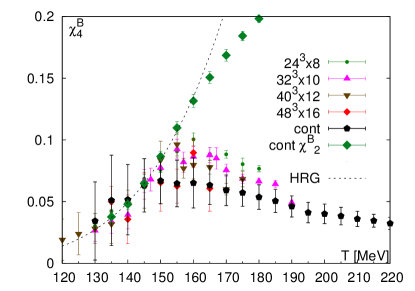
The baryon fourth moment shows milder lattice artefacts; here the large statistical errors dominate over the systematic errors (see Fig. 9). We also show since the second and fourth moment receive the same prediction from the HRG model, independently of how many baryons and mesons are included in the resonance list. The point where and are no longer consistent cannot be described by any resonance list. Multi-baryon states are expected to lead to , but here we observe the opposite from MeV. The relation motivates the concept that the free energy is dominated by objects with fractional baryon numbers: quarks. Given the trend of the HRG model, it is conceivable that the departure point from the HRG model, and the respective maximum of the fourth-order derivative ( or ) are very close in temperature.
V Results at high temperatures
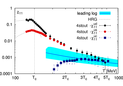
In this section we show our continuum extrapolated results at intermediate and high temperatures. The first observables are the off-diagonal quark flavor correlators, already shown in the transition region in Fig. 6. Increasing the temperature range (see Fig. 10), we actually see that the value of the light-light correlator spans more than two orders of magnitude between and . Between and the leading perturbative log, which was calculated at zero quark mass Blaizot et al. (2001), describes our data. Our data suggest that the light-charm correlator becomes compatible with the light-light correlator at about , but its agreement with the leading log starts a bit earlier. The mass of the strange quark is negligible in this observable already at a temperature 240 MeV.
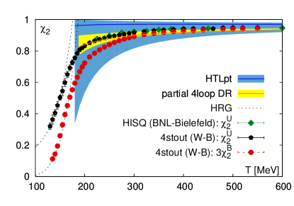
For the light quark number susceptibility (Fig. 11) there are continuum results available Borsanyi et al. (2012b); Bazavov et al. (2013a). Here we compare to the recent result with the HISQ action (with a combined analysis also using p4 data) Bazavov et al. (2013a). Our result is compatible with both Refs. Borsanyi et al. (2012b); Bazavov et al. (2013a) within errorbars. Here we also show the latest (improved) perturbative estimates, based on hard thermal loops (HTL) Haque et al. (2014a) and dimensional reduction (DR) Mogliacci et al. (2013). The improvement used in Ref. Mogliacci et al. (2013) has reduced the renormalization scale dependence enormously. Our data are approximately one sigma higher than the upper edge of the yellow band of the DR result. The central line of the band is calculated at the renormalization scale , the upper edge at and the lower edge at .
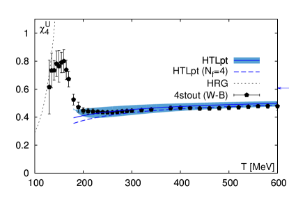
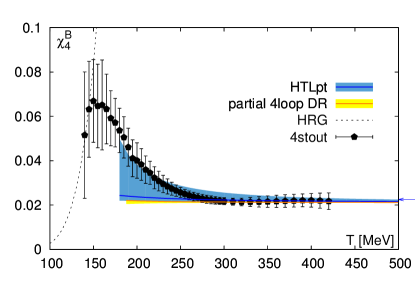
The fourth order cumulants at high and intermediate temperature are shown in Fig. 12. Both and are the fourth derivative of the free energy with respect to the chemical potential, the difference is that for the former the chemical potential is associated with only one of the quarks, whereas for the latter it is associated with all quarks at the same time. Here the HTL results have a very small renormalization scale dependence. The data confirms the HTL prediction that the Stefan-Boltzmann limit is (almost) reached for at intermediate temperatures, approaches it much slower. In both cases the improved and resummed perturbative results give an accurate description of lattice data above 250 MeV.
This agreement may seem trivial since the lattice result is continuum extrapolated and resummed perturbation theory is evaluated at high temperatures, both approaches are expected to solve QCD. There is a subtle difference, however, between HTL theory and lattice solutions. We simulated our ensembles with physical quark masses and 2+1+1 dynamical flavors. HTL results, on the other hand, are available for massless quarks only, and for as well as for . The mass of the strange quarks becomes irrelevant before we see agreement between lattice data and HTL. At intermediate temperatures the large mass of the charm makes the Hard Thermal Loop theory the closest match to our setting. In order to compare the same observables we do not count the baryon charge of the charm quark in and . To estimate the effect of the charm quark in the sea from the improved perturbation theory side we plot the three-flavor and four-flavor result for together in Fig. 12 (see Ref. Haque et al. (2014b)).
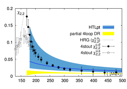
We close our discussion with the off-diagonal fourth order correlator. In Fig. 13 we show both the light-light and the light-strange correlator. Here the effect of the strange quark mass diminishes even sooner, at around 200 MeV. The agreement with the HTL result starts at a temperature MeV, in accordance with the other observables We also show the prediction of dimensional reduction Mogliacci et al. (2013).
VI Concluding remarks
In this paper we introduced our thermodynamics program with the four-level-smeared (4stout) staggered action. We focused on the fluctuations of conserved charges and updated our earlier result on second order fluctuations Borsanyi et al. (2012b). Since our first paper on fluctuations, we have introduced very fine lattices () in the transition range and extended the analysis to high temperatures where a comparison to resummed and improved perturbation theory is possible. We have also presented diagonal and off-diagonal fourth order cumulants. Here our data could be used to determine the lowest temperature for the three-loop HTL approximation: approx. 250 MeV.
We have studied whether the hadron resonance gas (HRG) model gives an adequate description of the fluctuation data. We find that well below the deconfinement temperature, i.e. around 130 MeV, all studied observables are well described by the HRG model. This was the most difficult to demonstrate for the fourth moment of the net charge distribution , which is a candidate for the freeze-out thermometer at the LHC. In this case, after adding a lattice to the analysis ( fm), our continuum extrapolation based on and 32 lattices is consistent with the HRG model prediction.
It is very likely that HRG does not describe all aspects of fluctuations in QCD thermodynamics below the transition. But for quantities for which it does one can introduce the highest temperature of agreement between lattice and HRG. This indicator of deconfinement is unavoidably model-dependent, even if one considers combinations that do not or only weakly depend on the actual list of resonances. This temperature can, however, be determined as long as the continuum limits are feasible with a sufficient precision. The data on our plots show in most cases an agreement up to , which can move to a lower temperature as our precision improves. This should not be confused with the limiting temperature of the Hagedorn spectrum, which can be higher. The temperature of highest agreement is not the same for all fluctuations as it was also suggested in Ref. Bellwied et al. (2013), e.g. and very possibly depart from the HRG estimates at lower temperatures. This may be a signal of the limitations of the HRG approach, but also suggests that the transition is a broad cross-over.
VII Acknowledgements
S. B. acknowledges the valuable discussions, correspondence and data exchange with Najmul Haque, Silvain Mogliacci, Mike Strickland, Nan Su and Aleksi Vuorinen.
This project was funded by the DFG grant SFB/TR55. S. D. Katz is funded by the ”Lendület” program of the Hungarian Academy of Sciences ((LP2012-44/2012). The work of R. Bellwied is supported through DOE grant DEFG02-07ER41521. Our code also uses the software package of Ref. Hernandez et al. (2005). An award of computer time was provided by the INCITE program. This research used resources of the Argonne Leadership Computing Facility, which is a DOE Office of Science User Facility supported under Contract DE-AC02-06CH11357. This research also used resources of the PRACE Research Infrastructure resource JUQUEEN at FZ-Jülich, Germany. The authors gratefully acknowledge the Gauss Centre for Supercomputing (GCS) for providing computing time for a GCS Large-Scale Project on the GCS share of the supercomputer JUQUEEN juq (2015) at Jülich Supercomputing Centre (JSC). For this research we also used the QPACE machine supported by the Deutsche Forschungsgesellschaft through the research program SFB TR55, and the GPU cluster at the Wuppertal University.
References
- Aoki et al. (2006a) Y. Aoki, G. Endrodi, Z. Fodor, S. Katz, and K. Szabo, Nature 443, 675 (2006a), arXiv:hep-lat/0611014 [hep-lat] .
- Aoki et al. (2006b) Y. Aoki, Z. Fodor, S. Katz, and K. Szabo, Phys.Lett. B643, 46 (2006b), arXiv:hep-lat/0609068 [hep-lat] .
- Aoki et al. (2009) Y. Aoki, S. Borsanyi, S. Durr, Z. Fodor, S. D. Katz, et al., JHEP 0906, 088 (2009), arXiv:0903.4155 [hep-lat] .
- Borsanyi et al. (2010a) S. Borsanyi et al. (Wuppertal-Budapest Collaboration), JHEP 1009, 073 (2010a), arXiv:1005.3508 [hep-lat] .
- Bazavov et al. (2012a) A. Bazavov, T. Bhattacharya, M. Cheng, C. DeTar, H. Ding, et al., Phys.Rev. D85, 054503 (2012a), arXiv:1111.1710 [hep-lat] .
- Jeon and Koch (2000) S. Jeon and V. Koch, Phys.Rev.Lett. 85, 2076 (2000), arXiv:hep-ph/0003168 [hep-ph] .
- Asakawa et al. (2000) M. Asakawa, U. W. Heinz, and B. Muller, Phys.Rev.Lett. 85, 2072 (2000), arXiv:hep-ph/0003169 [hep-ph] .
- Luo (2015) X. Luo, J.Phys.Conf.Ser. 599, 012023 (2015), arXiv:1501.03010 [nucl-ex] .
- Stephanov et al. (1999) M. A. Stephanov, K. Rajagopal, and E. V. Shuryak, Phys.Rev. D60, 114028 (1999), arXiv:hep-ph/9903292 [hep-ph] .
- Karsch and Redlich (2011) F. Karsch and K. Redlich, Phys.Lett. B695, 136 (2011), arXiv:1007.2581 [hep-ph] .
- Becattini et al. (2006) F. Becattini, J. Manninen, and M. Gazdzicki, Phys.Rev. C73, 044905 (2006), arXiv:hep-ph/0511092 [hep-ph] .
- Cleymans et al. (2006) J. Cleymans, H. Oeschler, K. Redlich, and S. Wheaton, Phys.Rev. C73, 034905 (2006), arXiv:hep-ph/0511094 [hep-ph] .
- Andronic et al. (2006) A. Andronic, P. Braun-Munzinger, and J. Stachel, Nucl.Phys. A772, 167 (2006), arXiv:nucl-th/0511071 [nucl-th] .
- Andronic et al. (2009) A. Andronic, P. Braun-Munzinger, and J. Stachel, Phys.Lett. B673, 142 (2009), arXiv:0812.1186 [nucl-th] .
- Becattini et al. (2014) F. Becattini, M. Bleicher, E. Grossi, J. Steinheimer, and R. Stock, (2014), arXiv:1405.0710 [nucl-th] .
- Adamczyk et al. (2014a) L. Adamczyk et al. (STAR Collaboration), Phys.Rev.Lett. 112, 032302 (2014a), arXiv:1309.5681 [nucl-ex] .
- Adamczyk et al. (2014b) L. Adamczyk et al. (STAR Collaboration), Phys.Rev.Lett. 113, 092301 (2014b), arXiv:1402.1558 [nucl-ex] .
- Bazavov et al. (2012b) A. Bazavov, H. Ding, P. Hegde, O. Kaczmarek, F. Karsch, et al., Phys.Rev.Lett. 109, 192302 (2012b), arXiv:1208.1220 [hep-lat] .
- Borsanyi et al. (2013a) S. Borsanyi, Z. Fodor, S. Katz, S. Krieg, C. Ratti, et al., Phys.Rev.Lett. 111, 062005 (2013a), arXiv:1305.5161 [hep-lat] .
- Borsanyi et al. (2014a) S. Borsanyi, Z. Fodor, S. Katz, S. Krieg, C. Ratti, et al., Phys.Rev.Lett. 113, 052301 (2014a), arXiv:1403.4576 [hep-lat] .
- Gottlieb et al. (1987) S. A. Gottlieb, W. Liu, D. Toussaint, R. Renken, and R. Sugar, Phys.Rev.Lett. 59, 2247 (1987).
- Gottlieb et al. (1988) S. A. Gottlieb, W. Liu, D. Toussaint, R. Renken, and R. Sugar, Phys.Rev. D38, 2888 (1988).
- Gavai et al. (1989) R. Gavai, J. Potvin, and S. Sanielevici, Phys.Rev. D40, 2743 (1989).
- Gavai et al. (2002) R. V. Gavai, S. Gupta, and P. Majumdar, Phys.Rev. D65, 054506 (2002), arXiv:hep-lat/0110032 [hep-lat] .
- Gavai and Gupta (2003) R. V. Gavai and S. Gupta, Phys.Rev. D67, 034501 (2003), arXiv:hep-lat/0211015 [hep-lat] .
- Allton et al. (2002) C. Allton, S. Ejiri, S. Hands, O. Kaczmarek, F. Karsch, et al., Phys.Rev. D66, 074507 (2002), arXiv:hep-lat/0204010 [hep-lat] .
- Bernard et al. (2005) C. Bernard et al. (MILC Collaboration), Phys.Rev. D71, 034504 (2005), arXiv:hep-lat/0405029 [hep-lat] .
- Gavai and Gupta (2006) R. Gavai and S. Gupta, Phys.Rev. D73, 014004 (2006), arXiv:hep-lat/0510044 [hep-lat] .
- Allton et al. (2005) C. Allton, M. Doring, S. Ejiri, S. Hands, O. Kaczmarek, et al., Phys.Rev. D71, 054508 (2005), arXiv:hep-lat/0501030 [hep-lat] .
- Datta et al. (2013) S. Datta, R. V. Gavai, and S. Gupta, Nucl.Phys. A904-905, 883c (2013), arXiv:1210.6784 [hep-lat] .
- Borsanyi et al. (2012a) S. Borsanyi, S. Durr, Z. Fodor, C. Hoelbling, S. D. Katz, et al., JHEP 1208, 126 (2012a), arXiv:1205.0440 [hep-lat] .
- Borsanyi et al. (2015a) S. Borsanyi, S. Durr, Z. Fodor, C. Holbling, S. D. Katz, et al., (2015a), arXiv:1504.03676 [hep-lat] .
- Giudice et al. (2014) P. Giudice, G. Aarts, C. Allton, A. Amato, S. Hands, et al., PoS LATTICE2013, 492 (2014), arXiv:1309.6253 [hep-lat] .
- Aarts et al. (2015) G. Aarts, C. Allton, A. Amato, P. Giudice, S. Hands, et al., JHEP 1502, 186 (2015), arXiv:1412.6411 [hep-lat] .
- Gattringer and Schadler (2015) C. Gattringer and H.-P. Schadler, Phys.Rev. D91, 074511 (2015), arXiv:1411.5133 [hep-lat] .
- Bazavov et al. (2012c) A. Bazavov et al. (HotQCD Collaboration), Phys.Rev. D86, 034509 (2012c), arXiv:1203.0784 [hep-lat] .
- Borsanyi et al. (2012b) S. Borsanyi, Z. Fodor, S. D. Katz, S. Krieg, C. Ratti, et al., JHEP 1201, 138 (2012b), arXiv:1112.4416 [hep-lat] .
- Borsanyi (2013) S. Borsanyi, Nucl.Phys. A904-905, 270c (2013), arXiv:1210.6901 [hep-lat] .
- Bellwied et al. (2013) R. Bellwied, S. Borsanyi, Z. Fodor, S. D. Katz, and C. Ratti, Phys.Rev.Lett. 111, 202302 (2013), arXiv:1305.6297 [hep-lat] .
- Bazavov et al. (2013a) A. Bazavov, H.-T. Ding, P. Hegde, F. Karsch, C. Miao, et al., Phys.Rev. D88, 094021 (2013a), arXiv:1309.2317 [hep-lat] .
- Dashen et al. (1969) R. Dashen, S.-K. Ma, and H. J. Bernstein, Phys.Rev. 187, 345 (1969).
- Venugopalan and Prakash (1992) R. Venugopalan and M. Prakash, Nucl.Phys. A546, 718 (1992).
- Karsch et al. (2003) F. Karsch, K. Redlich, and A. Tawfik, Phys.Lett. B571, 67 (2003), arXiv:hep-ph/0306208 [hep-ph] .
- Huovinen and Petreczky (2010) P. Huovinen and P. Petreczky, Nucl.Phys. A837, 26 (2010), arXiv:0912.2541 [hep-ph] .
- Borsanyi et al. (2014b) S. Borsanyi, Z. Fodor, C. Hoelbling, S. D. Katz, S. Krieg, et al., Phys.Lett. B730, 99 (2014b), arXiv:1309.5258 [hep-lat] .
- Bazavov et al. (2013b) A. Bazavov, H. T. Ding, P. Hegde, O. Kaczmarek, F. Karsch, et al., Phys. Rev. Lett. 111, 082301, 082301 (2013b), arXiv:1304.7220 [hep-lat] .
- Kajantie et al. (2003) K. Kajantie, M. Laine, K. Rummukainen, and Y. Schroder, Phys.Rev. D67, 105008 (2003), arXiv:hep-ph/0211321 [hep-ph] .
- Vuorinen (2003a) A. Vuorinen, Phys.Rev. D68, 054017 (2003a), arXiv:hep-ph/0305183 [hep-ph] .
- Vuorinen (2003b) A. Vuorinen, Phys.Rev. D67, 074032 (2003b), arXiv:hep-ph/0212283 [hep-ph] .
- Blaizot et al. (2003a) J. Blaizot, E. Iancu, and A. Rebhan, Phys.Rev. D68, 025011 (2003a), arXiv:hep-ph/0303045 [hep-ph] .
- Andersen et al. (2013) J. O. Andersen, S. Mogliacci, N. Su, and A. Vuorinen, Phys.Rev. D87, 074003 (2013), arXiv:1210.0912 [hep-ph] .
- Mogliacci et al. (2013) S. Mogliacci, J. O. Andersen, M. Strickland, N. Su, and A. Vuorinen, JHEP 1312, 055 (2013), arXiv:1307.8098 [hep-ph] .
- Braaten and Pisarski (1992) E. Braaten and R. D. Pisarski, Phys.Rev. D45, 1827 (1992).
- Andersen et al. (2002) J. O. Andersen, E. Braaten, E. Petitgirard, and M. Strickland, Phys.Rev. D66, 085016 (2002), arXiv:hep-ph/0205085 [hep-ph] .
- Andersen et al. (2010) J. O. Andersen, M. Strickland, and N. Su, JHEP 1008, 113 (2010), arXiv:1005.1603 [hep-ph] .
- Boyd et al. (1996) G. Boyd, J. Engels, F. Karsch, E. Laermann, C. Legeland, et al., Nucl.Phys. B469, 419 (1996), arXiv:hep-lat/9602007 [hep-lat] .
- Borsanyi et al. (2012c) S. Borsanyi, G. Endrodi, Z. Fodor, S. Katz, and K. Szabo, JHEP 1207, 056 (2012c), arXiv:1204.6184 [hep-lat] .
- Strickland et al. (2011) M. Strickland, J. O. Andersen, L. E. Leganger, and N. Su, Prog.Theor.Phys.Suppl. 187, 106 (2011), arXiv:1011.0416 [hep-ph] .
- Andersen et al. (2011) J. O. Andersen, L. E. Leganger, M. Strickland, and N. Su, Phys.Rev. D84, 087703 (2011), arXiv:1106.0514 [hep-ph] .
- Haque et al. (2013) N. Haque, M. G. Mustafa, and M. Strickland, JHEP 1307, 184 (2013), arXiv:1302.3228 [hep-ph] .
- Haque et al. (2014a) N. Haque, J. O. Andersen, M. G. Mustafa, M. Strickland, and N. Su, Phys.Rev. D89, 061701 (2014a), arXiv:1309.3968 [hep-ph] .
- Blaizot et al. (2001) J. Blaizot, E. Iancu, and A. Rebhan, Phys.Lett. B523, 143 (2001), arXiv:hep-ph/0110369 [hep-ph] .
- Blaizot et al. (2003b) J. Blaizot, E. Iancu, and A. Rebhan, Eur.Phys.J. C27, 433 (2003b), arXiv:hep-ph/0206280 [hep-ph] .
- Haque et al. (2014b) N. Haque, A. Bandyopadhyay, J. O. Andersen, M. G. Mustafa, M. Strickland, et al., JHEP 1405, 027 (2014b), arXiv:1402.6907 [hep-ph] .
- Bzdak et al. (2013) A. Bzdak, V. Koch, and V. Skokov, Phys.Rev. C87, 014901 (2013), arXiv:1203.4529 [hep-ph] .
- Skokov et al. (2013) V. Skokov, B. Friman, and K. Redlich, Phys.Rev. C88, 034911 (2013), arXiv:1205.4756 [hep-ph] .
- Alba et al. (2015) P. Alba, R. Bellwied, M. Bluhm, V. M. Sarti, M. Nahrgang, et al., (2015), arXiv:1504.03262 [hep-ph] .
- Kapusta and Gale (2006) J. I. Kapusta and C. Gale, Finite-Temperature Field Theory, 2nd ed. (Cambridge University Press, 2006) cambridge Books Online.
- Toimela (1983) T. Toimela, Phys.Lett. B124, 407 (1983).
- Hasenfratz and Karsch (1983) P. Hasenfratz and F. Karsch, Phys.Lett. B125, 308 (1983).
- Kaczmarek et al. (2014) O. Kaczmarek, C. Schmidt, P. Steinbrecher, and M. Wagner, (2014), arXiv:1411.4439 [physics.comp-ph] .
- Bali et al. (2010) G. S. Bali, S. Collins, and A. Schafer, Comput.Phys.Commun. 181, 1570 (2010), arXiv:0910.3970 [hep-lat] .
- Morningstar and Peardon (2004) C. Morningstar and M. J. Peardon, Phys.Rev. D69, 054501 (2004), arXiv:hep-lat/0311018 [hep-lat] .
- Davies et al. (2010) C. Davies, C. McNeile, K. Wong, E. Follana, R. Horgan, et al., Phys.Rev.Lett. 104, 132003 (2010), arXiv:0910.3102 [hep-ph] .
- Aoki et al. (2014) S. Aoki et al., Eur. Phys. J. C74, 2890 (2014), arXiv:1310.8555 [hep-lat] .
- Rosner and Stone (2013) J. L. Rosner and S. Stone, (2013), arXiv:1309.1924 [hep-ex] .
- Borsanyi et al. (2015b) S. Borsanyi, S. Dürr, Z. Fodor, et al., “Determination of from 2+1+1 flavor 4-stout staggered lattices,” (2015b), (in preparation).
- McNeile et al. (2010) C. McNeile, C. Davies, E. Follana, K. Hornbostel, and G. Lepage, Phys.Rev. D82, 034512 (2010), arXiv:1004.4285 [hep-lat] .
- Durr et al. (2011a) S. Durr, Z. Fodor, C. Hoelbling, S. Katz, S. Krieg, et al., Phys.Lett. B701, 265 (2011a), arXiv:1011.2403 [hep-lat] .
- Durr et al. (2011b) S. Durr, Z. Fodor, C. Hoelbling, S. Katz, S. Krieg, et al., JHEP 1108, 148 (2011b), arXiv:1011.2711 [hep-lat] .
- Borsanyi et al. (2013b) S. Borsanyi, S. Durr, Z. Fodor, S. Krieg, A. Schafer, et al., Phys.Rev. D88, 014513 (2013b), arXiv:1205.0788 [hep-lat] .
- Borsanyi et al. (2012d) S. Borsanyi, S. Durr, Z. Fodor, C. Hoelbling, S. D. Katz, et al., JHEP 1209, 010 (2012d), arXiv:1203.4469 [hep-lat] .
- Luscher (2010) M. Luscher, JHEP 1008, 071 (2010), arXiv:1006.4518 [hep-lat] .
- Borsanyi et al. (2010b) S. Borsanyi, G. Endrodi, Z. Fodor, A. Jakovac, S. D. Katz, et al., JHEP 1011, 077 (2010b), arXiv:1007.2580 [hep-lat] .
- Durr et al. (2008) S. Durr, Z. Fodor, J. Frison, C. Hoelbling, R. Hoffmann, et al., Science 322, 1224 (2008), arXiv:0906.3599 [hep-lat] .
- Borsanyi et al. (2015c) S. Borsanyi, S. Durr, Z. Fodor, C. Hoelbling, S. Katz, et al., Science 347, 1452 (2015c), arXiv:1406.4088 [hep-lat] .
- Akaike (1974) H. Akaike, IEEE Transactions on Automatic Control 19 (1974).
- Bazavov et al. (2014a) A. Bazavov, H. T. Ding, P. Hegde, O. Kaczmarek, F. Karsch, et al., Phys.Rev.Lett. 113, 072001 (2014a), arXiv:1404.6511 [hep-lat] .
- Olive et al. (2014) K. A. Olive et al. (Particle Data Group), Chin. Phys. C38, 090001 (2014).
- Bernard et al. (2006) C. Bernard, M. Golterman, and Y. Shamir, Phys.Rev. D73, 114511 (2006), arXiv:hep-lat/0604017 [hep-lat] .
- Ejiri (2008) S. Ejiri, Phys.Rev. D78, 074507 (2008), arXiv:0804.3227 [hep-lat] .
- Bazavov et al. (2014b) A. Bazavov, H. T. Ding, P. Hegde, O. Kaczmarek, F. Karsch, et al., Phys.Lett. B737, 210 (2014b), arXiv:1404.4043 [hep-lat] .
- Petreczky et al. (2009) P. Petreczky, P. Hegde, and A. Velytsky (RBC-Bielefeld Collaboration), PoS LAT2009, 159 (2009), arXiv:0911.0196 [hep-lat] .
- Ejiri et al. (2009) S. Ejiri, F. Karsch, E. Laermann, C. Miao, S. Mukherjee, et al., Phys.Rev. D80, 094505 (2009), arXiv:0909.5122 [hep-lat] .
- Kaczmarek et al. (2011) O. Kaczmarek, F. Karsch, E. Laermann, C. Miao, S. Mukherjee, et al., Phys.Rev. D83, 014504 (2011), arXiv:1011.3130 [hep-lat] .
- Friman et al. (2011) B. Friman, F. Karsch, K. Redlich, and V. Skokov, Eur.Phys.J. C71, 1694 (2011), arXiv:1103.3511 [hep-ph] .
- Engels et al. (2003) J. Engels, L. Fromme, and M. Seniuch, Nucl.Phys. B675, 533 (2003), arXiv:hep-lat/0307032 [hep-lat] .
- Hernandez et al. (2005) V. Hernandez, J. E. Roman, and V. Vidal, ACM Trans. Math. Software 31, 351 (2005).
- juq (2015) JUQUEEN: IBM Blue Gene/Q Supercomputer System at the Jülich Supercomputing Centre, Tech. Rep. 1 A1 (Jülich Supercomputing Centre, http://dx.doi.org/10.17815/jlsrf-1-18, 2015).