Dark matter (stellar, interstellar, galactic, and cosmological) Elementary particle processes Extensions of electroweak Higgs sector

Dwarf Galaxy $\gamma$-excess and 3.55 keV X-ray Line In A Nonthermal Dark Matter Model

Abstract

Recent data from Reticulum II (RetII) require the energy range of the FermiLAT $\gamma$-excess to be $\sim$ $2-10$ GeV. We adjust our unified nonthermal Dark Matter (DM) model to accommodate this. We have two extra scalars beyond the Standard Model to also explain 3.55 keV X-ray line. Now the mass of the heavier of them has to be increased to lie around 250 GeV, while that of the lighter one remains at 7.1 keV. This requires a new seed mechanism for the $\gamma$-excess and new Boltzmann equations for the generation of the DM relic density. All concerned data for RetII and the X-ray line can now be fitted well and consistency with other indirect limits attained.

The endeavour for the detection of Dark Matter (DM) is increasingly gaining momentum. Gamma-ray signals from the FermiLAT experiment have attracted much attention [[1]-[12]]. These cannot be explained by the known astrophysical processes. On the other hand, their DM origin has been a topic of debate [[12]-[42]]. One possibility is the decay/self-annihilation of DM particles clustered around massive gravitating bodies, e.g. the Galactic Centre (GC) or dwarf galaxies. Separately, an X-ray line of energy 3.55 keV has been reported [[43], [44]] by the XMM Newton observatory by use of a data set obtained from Andromeda and 73 other galaxy clusters including Perseus. An astrophysical explanation [45] of this line, though possible, is beset [46] with uncertainties in the potassium abundance in the target. Thus a DM origin of the X-ray line remains a viable possibility and could be from decaying [[47], [48]] annihilating [49] or excited [50] DM. It would be a worthwhile effort to construct a unified DM model for these two phenomena.

Data from the dwarf spheroidal galaxy RetII [12] suggest an upward shift in the earlier claimed [[2]-[9]] energy range of the FermiLAT $\gamma$-excess to $2-10$ GeV. The high galactic latitude of RetII makes its $\gamma$-emission relatively free from complicated backgrounds. This higher range is what we adopt here. That requires a modification in our 2-component nonthermal DM model [36], proposed earlier to explain both the $\gamma$-excess and the X-ray line. In our model the fields describing DM have tiny couplings with Standard Model (SM) fields. As a result, the DM particles are produced nonthermally and they are unable to thermalise later. Two extra electroweak (EW) singlet scalar fields $S_{{}_{2,\,3}}$ are introduced. These and the SU(2)_L doublet Higgs field $H$ comprise the scalar sector. Inter-mixing among them leads to three physical particles $\chi_{{}_{{}_{1,\,2,\,3}}}$ with $M_{\chi_{{}_{{}_{1}}}}\sim 125$ GeV, $\chi_{{}_{{}_{2}}}$ and $\chi_{{}_{{}_{3}}}$ (with $M_{\chi_{{}_{{}_{3}}}}\sim 7$ keV) having tiny mixing angles between them. The decays $\chi_{{}_{{}_{3}}}\rightarrow\gamma\gamma$ and $\chi_{{}_{{}_{2}}}\rightarrow{\rm b}\bar{\rm b}$ (with the ${\rm b}$’s emitting neutral pions via hadronisation) respectively account for the X-ray line and $\gamma$-excess. Relic DM, a mixture of $\chi_{{}_{{}_{2}}}$ and $\chi_{{}_{{}_{3}}}$, forms after EW symmetry breaking through the processes $\chi_{{}_{{}_{1}}}\rightarrow\chi_{{}_{{}_{2,\,3}}}\chi_{{}_{{}_{2,\,3}}}$, $W^{+}W^{-}\rightarrow\chi_{{}_{{}_{2,\,3}}}\chi_{{}_{{}_{2,\,3}}}$, $ZZ\rightarrow\chi_{{}_{{}_{2,\,3}}}\chi_{{}_{{}_{2,\,3}}}$, $t\bar{t}\rightarrow\chi_{{}_{{}_{2,\,3}}}\chi_{{}_{{}_{2,\,3}}}$, $\chi_{{}_{{}_{1}}}\chi_{{}_{{}_{1}}}\rightarrow\chi_{{}_{{}_{2,\,3}}}\chi_{{}_{{}_{2,\,3}}}$.

An important feature here is the sensitive link between $M_{\chi_{{}_{{}_{2}}}}$ and the energy spectrum of the $\gamma$-excess. Indeed, we need $M_{\chi_{{}_{{}_{2}}}}$ in the ballpark of 250 GeV to fit the increased energy range of this excess. As shown numerically later, too small a magnitude of $M_{\chi_{{}_{{}_{2}}}}$, as compared with this ballpark value, would unacceptably shift the energy spectrum of the $\gamma$-excess to a lower range. On the other hand, too large a mass of $\chi_{{}_{{}_{2}}}$ would inhibit its pair production which took place after the EW phase transition ($T_{W}\sim 153$ GeV [51]). Now the decay $\chi_{{}_{{}_{1}}}\rightarrow\chi_{{}_{{}_{2}}}\chi_{{}_{{}_{2}}}$ is disallowed and $\chi_{{}_{{}_{2}}}$’s are produced in the early Universe from the pair annihilation of SM fermions and gauge bosons. Moreover, the decay $\chi_{{}_{{}_{2}}}\rightarrow W^{+}W^{-}$ is now allowed. The strength of the $\chi_{{}_{{}_{2}}}W^{+}W^{-}$ ($\chi_{{}_{{}_{2}}}{\rm b}\bar{\rm b}$) coupling is proportional to $M^{2}_{W}/v$ ($gm_{\rm b}/M_{W}$), $g$ being the SU(2)_L gauge coupling. Consequently, the $\chi_{{}_{{}_{2}}}\rightarrow W^{+}W^{-}$ decay channel becomes the dominant contribution to our seed mechanism for the $\gamma$-excess.

Let us recount the salient features of our model. The stability of all scalar fields is ensured by the discrete symmetry $\mathbb{Z}_{2}\times\mathbb{Z}^{\prime}_{2}$. With respect to this, $S_{{}_{2}}$ and $S_{{}_{3}}$ have charges (-1, 1) and (1, -1) respectively, while those of all other SM fields are (1, 1). The scalar potential for the Higgs portal is given by $V=V_{0}+V^{\prime}$ where

$$V_{0}(H,S_{{}_{2}},S_{{}_{3}}) = \kappa_{{}_{1}}(H^{\dagger}H-\frac{1}{2}v^{2})^{2}+\frac{1}{4}\kappa_{{}_{2}}S_{{}_{2}}^{4}$$

$$+\frac{1}{4}\kappa_{{}_{3}}(S_{{}_{3}}^{2}-u^{2})^{2}+\frac{1}{2}\rho_{{}_{2}}^{2}S_{{}_{2}}^{2}$$

$$+\lambda_{12}(H^{\dagger}H)S_{{}_{2}}^{2}+\lambda_{23}S_{{}_{2}}^{2}S_{{}_{3}}^{2}$$

$$+\leavevmode\nobreak\ \lambda_{13}(H^{\dagger}H-\frac{1}{2}v^{2})(S_{{}_{3}}^{2}-u^{2})\,\,,$$

$$V^{\prime}(S_{{}_{2}},S_{{}_{3}}) = \alpha\,S_{{}_{2}}S_{{}_{3}}\,\,.$$ (1)

Terms such as $(H^{\dagger}H)S_{{}_{2}}S_{{}_{3}}$, $S_{{}_{2}}^{3}S_{{}_{3}}$, $S_{{}_{2}}S_{{}_{3}}^{3}$ are excluded by the assumed symmetry. The “small” $V^{\prime}$ term softly and explicitly breaks the $\mathbb{Z}_{2}\times\mathbb{Z}^{\prime}_{2}$ invariance down to that of $\mathbb{Z}^{\prime\prime}_{2}$ under which $S_{{}_{2,\,3}}$ are odd and the rest are even. This $\mathbb{Z}^{\prime\prime}_{2}$ is spontaneously broken by the VEV $u$ ($2\,{\rm MeV}<u\leq 10\,{\rm MeV}$) of $S_{{}_{3}}$. In (1) $v=\langle\rm Re\,H^{0}\rangle$, $H^{0}$ being the neutral member of the doublet $H$, while the coupling constants $\kappa_{1,2,3}$, $\rho_{2}$, $\lambda_{12}$, $\lambda_{23}$ and $\lambda_{13}$ obey certain stability conditions detailed in Ref. [36]. Domain wall formation from the restoration of $\mathbb{Z}^{\prime\prime}_{2}$ at a high temperature can also be shown to be inconsequential [51].

The physical scalar fields are $s_{1}=\sqrt{2}{\rm Re}\,H^{0}-v$, $s_{{}_{2}}=S_{{}_{2}}$ and $s_{{}_{3}}=S_{{}_{3}}-u$ with their squared mass matrix

$$\mathcal{M}^{2}=\left(\begin{array}[]{ccc}2\kappa_{{}_{1}}v^{2}&0&2\lambda_{13}uv\\ 0&\rho_{{}_{2}}^{2}+\lambda_{12}v^{2}+2\lambda_{23}u^{2}&\alpha\\ 2\lambda_{13}uv&\alpha&2\kappa_{{}_{3}}u^{2}\\ \end{array}\right)\,.$$ (5)

The eigenvalues of (5) are $M^{2}_{\chi_{{}_{{}_{1,\,2,\,3}}}}$ with respective eigenstate fields $\chi_{{}_{{}_{1,\,2,\,3}}}$. The latter are linearly related to $s_{{}_{1,\,2,\,3}}$ via the mixing angles $\theta_{12}$, $\theta_{23}$ and $\theta_{13}$. These angles are quite tiny because two of them come from symmetry breaking also owing to the smallness of the $\lambda$’s. $\theta_{23}$ is a pure $\mathbb{Z}_{2}\times\mathbb{Z}^{\prime}_{2}$ symmetry breaking parameter controlled by $\alpha$ which is chosen to be $\sim$ ($10^{-9}-10^{-8}$) GeV² while $\theta_{12}$ is generated by an interplay of $\alpha$ and $\lambda_{13}$ which has been taken $\sim 10^{-9}$. The last mixing angle $\theta_{13}$ arises from the spontaneous breakdown of the $\mathbb{Z}^{\prime\prime}_{2}$ symmetry driven by $\lambda_{13}$. From a UV perspective the smallness of $\alpha$ and the $\lambda$’s could be due to a presumed hidden tree level symmetry broken by radiative loop corrections. We further choose $M_{\chi_{{}_{{}_{1}}}}=125.5$ GeV $M_{\chi_{{}_{{}_{2}}}}\sim 250\,{\rm GeV}$ and $M_{\chi_{{}_{{}_{3}}}}=7.1$ keV. The last choice is consistent with an $\mathcal{O}$ (MeV) $u$ provided $2\times 10^{-7}<\kappa_{3}<4\times 10^{-6}$. However, the upper bound is further restricted to $\sim 7\times 10^{-7}$ if we take the $\chi_{{}_{{}_{3}}}$ self-interaction cross section $\sigma_{\chi_{{}_{{}_{3}}}}$ divided by its mass $M_{\chi_{{}_{{}_{3}}}}$ to be less than 0.47 cm${}^{2}/g$ from collisions between different galaxy clusters [52], cf. Fig.1. The corresponding quantity for $\chi_{{}_{{}_{2}}}$ is too small to make any difference.

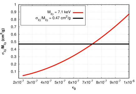
Figure 1: Variation of ${\sigma_{\chi_{{}_{{}_{3}}}}}/{M_{\chi_{{}_{{}_{3}}}}}$ with $\kappa_{3}$.

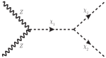
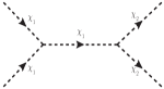
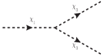
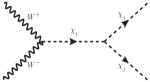
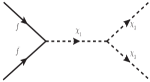
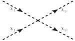
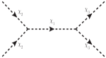
Figure 2: Feynman diagrams for dominant production channels of both the dark matter components $\chi_{{}_{{}_{2}}}$ and $\chi_{{}_{{}_{3}}}$.

Both $\chi_{{}_{{}_{2}}}$ and $\chi_{{}_{{}_{3}}}$ got produced nonthermally in the early Universe but only after EW symmetry breaking. Thereafter, the self-annihilation of $W$, $Z$, $\chi_{{}_{{}_{1}}}$ and $t$ (see Fig.2) acted as primary sources of DM particles $\chi_{{}_{{}_{2,\,3}}}$. The decay $\chi_{{}_{{}_{1}}}\rightarrow\chi_{{}_{{}_{3}}}\chi_{{}_{{}_{3}}}$ also contributed. Let $Y_{\chi_{{}_{{}_{j}}}}$ be the comoving number density (= actual number density $\div$ entropy density of the Universe) of $\chi_{{}_{{}_{j}}}$. It is given as a function of $z\equiv\frac{M_{\chi_{{}_{{}_{1}}}}}{T}$ by a set of two coupled Boltzmann equations. The latter involve the thermally averaged decay width $\langle\Gamma_{\chi_{{}_{{}_{1}}}\rightarrow\chi_{{}_{{}_{3}}}\chi_{{}_{{}_{3}}}}\rangle$ as well as the pair-production cross section times the relative velocity of collision ${\langle\sigma{\rm v}\rangle}_{x\bar{x}\rightarrow\chi_{{}_{{}_{2,\,3}}}\chi_{{}_{{}_{2,\,3}}}}$ for $x=W$, $Z$, $f$ and $\chi_{{}_{{}_{1,\,2}}}$. Details appear in Ref. [36] and will not be repeated here. The only change is that the decay $\chi_{{}_{{}_{1}}}\rightarrow\chi_{{}_{{}_{2}}}\chi_{{}_{{}_{2}}}$ is disallowed now. Thus, while the equation for $\frac{dY_{\chi_{{}_{{}_{3}}}}}{dz}$ is unchanged, that for $\frac{dY_{\chi_{{}_{{}_{2}}}}}{dz}$ is changed to

$$\!\!\!\!\!\!\!\!\!\!\!\!\frac{dY_{\chi_{{}_{{}_{2}}}}}{dz}=-\leavevmode\nobreak\ \frac{4\pi^{2}}{45\times 1.66}M_{pl}\,M_{\chi_{{}_{{}_{1}}}}\sqrt{g_{\star}(T)}\,\,{z^{-2}}\,\,\times$$

$$\!\!\!\!\!\!\!\!\!\!\!\!\left(\sum_{a}\,({{Y}^{2}_{\chi_{{}_{{}_{2}}}}}-{Y^{eq}_{a}}\,^{2})\,\langle{\sigma{\rm v}}\rangle_{a\bar{a}\rightarrow\chi_{{}_{{}_{2}}}\chi_{{}_{{}_{2}}}}\,+\leavevmode\nobreak\ Y^{2}_{\chi_{{}_{{}_{2}}}}\,\,\langle{\sigma{\rm v}}\rangle_{\chi_{{}_{{}_{2}}}\chi_{{}_{{}_{2}}}\rightarrow\chi_{{}_{{}_{3}}}\chi_{{}_{{}_{3}}}}\right)$$

(6)

with $a=W$, $Z$, $f$ and $\chi_{{}_{{}_{1}}}$. Further, the DM relic density is given (for $j=2$, $3$) by

$$\Omega_{\chi_{{}_{{}_{j}}}}h^{2}=2.755\times 10^{8}\,(M_{\chi_{{}_{{}_{j}}}}/{\rm GeV})\,Y_{\chi_{{}_{{}_{j}}}}(z_{0})\,,$$ (7)

where $z_{0}\equiv M_{\chi_{{}_{{}_{1}}}}/{T_{0}}$, $T_{0}$ being the present temperature of the Universe.

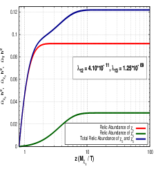
(a) $\Omega_{\chi_{{}_{{}_{2}}}}>\Omega_{\chi_{{}_{{}_{3}}}}$

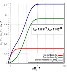
(b) $\Omega_{\chi_{{}_{{}_{2}}}}<\Omega_{\chi_{{}_{{}_{3}}}}$

Figure 3: Variation of relic densities of both the dark matter candidates with $z$.

We take as a boundary condition the vanishing of $Y_{\chi_{{}_{{}_{j}}}}$ at the EW phase transition ($z\sim 0.83$). Figures 3(a) and 3(b) show the variation of the relic densities of both DM candidates $\chi_{{}_{{}_{2,\,3}}}$ with $z$ for different values of $\lambda_{12}$, $\lambda_{13}$ which are $\sim 10^{-9}-10^{-11}$. Such strengths are needed to keep $Y_{\chi_{{}_{{}_{2,\,3}}}}$ small enough to generate the right DM relic density ($\Omega_{\rm DM}h^{2}$) at the present epoch. Appropriate values have been chosen for $\lambda_{12}$, $\lambda_{13}$ depending on whether $\chi_{{}_{{}_{2}}}$ or $\chi_{{}_{{}_{3}}}$ is the dominant DM component. Starting with null values, $Y_{\chi_{{}_{{}_{2,\,3}}}}$ are seen to rise as more and more DM is produced from the decay/self-annihilation of SM particles. They eventually saturate to respective particular values at $z\sim 10$ corresponding to a temperature $T\sim 12$ GeV of the Universe, depending on the particular values of $\lambda_{12}$, $\lambda_{13}$. These saturation values together need to satisfy the PLANCK [53] 68% c.l. constraint $0.1172\leq\Omega_{\rm DM}h^{2}\leq 0.1226$. Contributions from individual pair production channels of $\chi_{{}_{{}_{2}}}$ towards $\Omega_{\chi_{{}_{{}_{2}}}}h^{2}$ are graphically shown in Fig.4 with chosen parameters given in its legend: blue line for $\chi_{{}_{{}_{1}}}$, green line for $Z$, red line for $W$ and brown line for t-quarks, the last being somewhat less in magnitude. The total relic density of $\chi_{{}_{{}_{2}}}$ (yellow line) saturates around 0.06 which is half the total DM relic density ($\Omega_{\rm T}h^{2}$) of today, cf. Ref. [53]. The remainder comes from $\chi_{{}_{{}_{3}}}$.

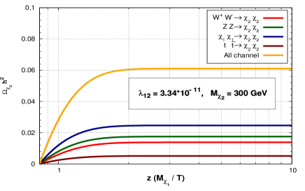
Figure 4: Contributions of different production channels to the relic density of a 300 GeV $\chi_{{}_{{}_{2}}}$ .

The allowed ranges of $\lambda_{12}$, $\lambda_{13}$, $\lambda_{23}$, $\theta_{12}$, $\theta_{13}$, $\theta_{23}$ are given in Table 1.

$\lambda_{12}$	$\lambda_{13}$	$\lambda_{23}$
$\sim(1.4-4.5)$	$\sim(0.7-2.4)$	$\sim(0.2-4.7)$
$\times 10^{-11}$	$\times 10^{-9}$	$\times 10^{-6}$
$\theta_{12}$	$\theta_{13}$	$\theta_{23}$
(rad)	(rad)	(rad)
$\sim(0.001-1.75)$	$\sim(0.063-6.3)$	$\sim(0.08-1.31)$
$\times 10^{-25}$	$\times 10^{-12}$	$\times 10^{-13}$

Table 1: Allowed ranges of concerned couplings and mixing angles. Also, $\alpha\sim(10^{-9}-10^{-8})$ GeV².

Given the chosen values of $M_{\chi_{{}_{{}_{3}}}}$ and $u$, the range of $\lambda_{23}$ is fixed by the need to avoid a late time decay of $\chi_{{}_{{}_{2}}}$ via $\chi_{{}_{{}_{2}}}\rightarrow\chi_{{}_{{}_{3}}}\chi_{{}_{{}_{3}}}$. The tiny magnitudes of $\theta_{13}$, $\theta_{23}$ and $\theta_{12}$ are required by the constraint of keeping the off diagonal elements of ${\mathcal{M}}^{2}$ in (5) to be very small. Further, the couplings of $\chi_{{}_{{}_{2,\,3}}}$ with $\chi_{{}_{{}_{1}}}$, which are functions of the three $\lambda$’s and the three $\theta$’s [36], remain sufficiently feeble to keep the former beyond the reach of DM direct detection experiments [[54]-[55]]. Another point to note is that $\chi_{{}_{{}_{2}}}$ behaves like a feebly interacting massive particle (FIMP) starting with a vanishing number density. Its fractional relic density saturates after increasing initially (cf. Fig.3a) as the temperature falls in the cooling Universe. This is the hallmark of a “freeze-in” behaviour [56], as contrasted with that of a WIMP; the relic density of the latter starts from an equilibrium nonzero value, decreases and then freezes out at a saturation level. Though much lighter, $\chi_{{}_{{}_{3}}}$ also freezes in a way similar to that of $\chi_{{}_{{}_{2}}}$ (cf. Fig.3b).

We turn next to the $\gamma$-excess observed from RetII covering the range $2-10$ GeV of the FermiLAT $\gamma$-energy spectrum. With $M_{\chi_{{}_{{}_{2}}}}\sim 250$ GeV, $\chi_{{}_{{}_{2}}}$ $-$ on account of its nonzero mixing with the SM-like Higgs boson $\chi_{{}_{{}_{1}}}$ $-$ decays predominately into $W^{+}W^{-}$. Because of the small $\chi_{{}_{{}_{1}}}\chi_{{}_{{}_{2}}}\chi_{{}_{{}_{2}}}$ coupling, $\chi_{{}_{{}_{2}}}$ pair-annihilation into the same final state, via s-channel $\chi_{{}_{{}_{1}}}$ exchange, is a negligible competitor. Ours is the first model explaining the RetII $\gamma$-excess from the decay $\chi_{{}_{{}_{2}}}\rightarrow W^{+}W^{-}$ with $\gamma$-rays coming predominantly out of neutral pions hadronising from $W^{\pm}$ decaying into $q\bar{q^{\prime}}$ pairs. Consider the $\gamma$-flux from RetII at a line of sight distance $\mathfrak{s}$ and subtending a solid angle $\Delta\Omega$. The differential distribution is

$$\frac{d\Phi_{\gamma}}{d\Omega dE} = \frac{1}{4\pi\,M_{\chi_{{}_{{}_{2}}}}}\leavevmode\nobreak\ \bar{J}\leavevmode\nobreak\ \Gamma^{\prime}_{\chi_{{}_{{}_{2}}}\rightarrow{W^{+}}{W^{-}}}\frac{dN^{W}_{\gamma}}{dE}\,\,.$$ (8)

Here $\frac{dN^{W}_{\gamma}}{dE}$ is the energy distribution of each of the two $\gamma$’s of energy $E$ produced from the $W$ pair, taken numerically from Ref. [57]. $\bar{J}=\frac{J}{\Delta\Omega}$ represents an average of the “astrophysical factor” $J$ [58] over the opening solid angle $\Delta\Omega=2\pi(1-\cos\alpha_{\rm int})$, the integration angle $\alpha_{\rm int}$ being $0.5^{0}$ [12]. Further,

$$J=\int\int\rho(\mathfrak{s},\Omega)d\mathfrak{s}\,d\Omega\,\,,$$ (9)

where $\rho(\mathfrak{s},\Omega)$ describes the variation of the local dark matter density in the neighbourhood of RetII. $J$ has been taken to be $10^{18.8}$ GeV cm^-2 from Ref. [58]. Finally, ${\Gamma^{\prime}}_{\chi_{{}_{{}_{2}}}\rightarrow{W}^{+}{W}^{-}}$ is the product of the partial width for the decay ${\chi_{{}_{{}_{2}}}\rightarrow{W}^{+}{W}^{-}}$ and the fractional relic density for the component $\chi_{{}_{{}_{2}}}$, i.e. ${\Gamma^{\prime}}_{\chi_{{}_{{}_{2}}}\rightarrow{\rm W}{\rm W}}=\frac{\Omega_{\chi_{{}_{{}_{2}}}}}{\Omega_{\rm T}}\Gamma_{\chi_{{}_{{}_{2}}}\rightarrow WW}$. Its occurrence in (8) is necessitated by the two component nature of our DM. The partial width, mentioned above, is given in a transparent notation by

$$\Gamma_{\chi_{{}_{{}_{2}}}\rightarrow W^{+}W^{-}}=\frac{g^{2}_{{\!}_{WW\chi_{{}_{{}_{2}}}}}}{64\pi}{M^{3}_{\chi_{{}_{{}_{2}}}}}(1-4{M^{2}_{W}}{M^{-2}_{\chi_{{}_{{}_{2}}}}})^{1/2}\times$$

$${M^{-4}_{W}}(1-4{M^{2}_{W}}{M^{-2}_{\chi_{{}_{{}_{2}}}}}+12{M^{4}_{W}}{M^{-4}_{\chi_{{}_{{}_{2}}}}})\,$$ (10)

with the coupling $g_{{\!}_{WW\chi_{{}_{{}_{2}}}}}$ given by

$$-\frac{2M^{2}_{W}}{v}(\sin\theta_{12}\cos\theta_{23}+\cos\theta_{12}\sin\theta_{23}\sin\theta_{13})\,$$

with $v=2^{-\frac{1}{4}}G^{-\frac{1}{2}}_{F}$, $G_{F}$ being the Fermi constant.

The $\gamma$-flux, computed from (8), (9) and (10) for each of the three different values of $M_{\chi_{{}_{{}_{2}}}}$, is plotted in Fig.5 in comparison with the data points. The background $\gamma$-flux [12] (turquoise line) is also shown. Though the computed plots have been generated with $\Gamma^{\prime}_{\chi_{{}_{{}_{2}}}\rightarrow W^{+}W^{-}}$ fixed at $6.27\times 10^{-27}$ s^-1, the fit does not change much, as seen by varying the latter through $\pm 0.94\times 10^{-27}$ s^-1. In order to produced the above mentioned range of values of $\Gamma^{\prime}_{\chi_{{}_{{}_{2}}}\rightarrow W^{+}W^{-}}$ the soft $\mathbb{Z}_{2}\times\mathbb{Z}^{\prime}_{2}$ symmetry breaking parameter $\alpha$ needs to be in the range $10^{-9}\,\,{\rm GeV}^{2}\mathrel{\mathchoice{\vbox{\offinterlineskip\halign{\hfil$\displaystyle#$\hfil\cr<\cr\sim\cr}}}{\vbox{\offinterlineskip\halign{\hfil$\textstyle#$\hfil\cr<\cr\sim\cr}}}{\vbox{\offinterlineskip\halign{\hfil$\scriptstyle#$\hfil\cr<\cr\sim\cr}}}{\vbox{\offinterlineskip\halign{\hfil$\scriptscriptstyle#$\hfil\cr<\cr\sim\cr}}}}\alpha\mathrel{\mathchoice{\vbox{\offinterlineskip\halign{\hfil$\displaystyle#$\hfil\cr<\cr\sim\cr}}}{\vbox{\offinterlineskip\halign{\hfil$\textstyle#$\hfil\cr<\cr\sim\cr}}}{\vbox{\offinterlineskip\halign{\hfil$\scriptstyle#$\hfil\cr<\cr\sim\cr}}}{\vbox{\offinterlineskip\halign{\hfil$\scriptscriptstyle#$\hfil\cr<\cr\sim\cr}}}}10^{-8}\,\,{\rm GeV}^{2}$. Clearly, the fit is worse when $M_{\chi_{{}_{{}_{2}}}}$ becomes 200 GeV. We have not extended our fits to cover $\chi_{{}_{{}_{2}}}$ much beyond 300 GeV since the production of $\chi_{{}_{{}_{2}}}$ (say from $t\bar{t}$ at the EW transition temperature $\sim$ 153 GeV) is then cut off by phase space.

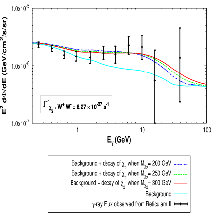
Figure 5: Energy distribution of the signal for three different $M_{\chi_{{}_{{}_{2}}}}$’s.

Let us discuss indirect constraints on $\Gamma^{\prime}_{\chi_{{}_{{}_{2}}}\rightarrow W^{+}W^{-}}$ from other observations. First, consider the limit from the positron flux in the AMS-02 data [59]. Using this data and assuming a single component DM, Ibarra et al. [60] plotted a lower limit (their Fig.3) on the partial lifetime $\Gamma^{-1}_{{\rm DM}\rightarrow W^{+}W^{-}}$ of the DM particle decaying into $W^{+}W^{-}$ as a function of the DM mass. Since we have a two-component DM in our scenario, we need to consider $\Gamma^{\prime}_{\chi_{{}_{{}_{2}}}\rightarrow W^{+}W^{-}}$ instead of $\Gamma_{\chi_{{}_{{}_{2}}}\rightarrow W^{+}W^{-}}$. (Note that the latter reduces to the former when $\Omega_{\chi_{{}_{{}_{2}}}}/\Omega_{\rm T}=1$ i.e. one has a single component DM scenario.) We convert the results of Ref. [60] into a plot of the upper limit on $\Gamma^{\prime}_{\chi_{{}_{{}_{2}}}\rightarrow W^{+}W^{-}}$ as a function of the $\chi_{{}_{{}_{2}}}$ fractional relic density $\Omega_{\chi_{{}_{{}_{2}}}}/\Omega_{\rm T}$ for $M_{\chi_{{}_{{}_{2}}}}=250$ GeV, 300 GeV. These plots are shown in Fig.6. Note that our chosen value of $6.27\times 10^{-27}\,{\rm s}^{-1}$ for $\Gamma^{\prime}_{\chi_{{}_{{}_{2}}}\rightarrow W^{+}W^{-}}$, made in order to fit the data from RetII, is below (cf. Fig.6) the range of this upper bound so long as $\Omega_{\chi_{{}_{{}_{2}}}}/\Omega_{\rm T}$ is less than $\sim 0.65\,(0.9)$ for $M_{\chi_{{}_{{}_{2}}}}=250\,{\rm GeV}\,(300\,{\rm GeV})$. Therefore, $\Omega_{\chi_{{}_{{}_{2}}}}$ in our model is constrained to be less than $\sim 0.65\,(0.9)$ times the total relic density $\Omega_{\rm T}$ for $M_{\chi_{{}_{{}_{2}}}}=250\,{\rm GeV}\,(300\,{\rm GeV})$.

Figure 6: ${\Gamma^{\prime}}_{\chi_{{}_{{}_{2}}}\rightarrow W^{+}W^{-}}$ plotted against $\Omega_{\chi_{{}_{{}_{2}}}}/\Omega_{\rm T}$: AMS-02 upper bound (red for $M_{\chi_{{}_{{}_{2}}}}=300$ GeV and green for $M_{\chi_{{}_{{}_{2}}}}=250$ GeV) as well as our fixed value (black line).

We next turn to the ANTARES [61] null result on the observation of muon neutrinos and antineutrinos from DM processes at the Galactic Centre. They derived a 90% c.l. upper bound on the total flux $\Phi_{\nu_{\mu}+\bar{\nu}_{\mu}}$ as a function of the mass of the DM particle taking its pair-annihilation into ${\rm b}\bar{\rm b}$ as the dominant subprocess. This is reproduced in the left panel of Fig.7. In our case the dominant subprocess is the decay $\chi_{{}_{{}_{2}}}\rightarrow W^{+}W^{-}$. The muon neutrino plus antineutrino flux from RetII, consequent upon the decays of the $W$’s, is plotted against $M_{\chi_{{}_{{}_{2}}}}$ in the right panel of Fig.7. Evidently our flux, being several orders of magnitude lower, is well within the ANTARES limit.

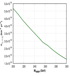
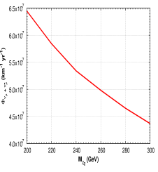
Figure 7: (a) ANTARES upper bound on $\Phi_{\nu_{\mu}+\bar{\nu}_{\mu}}$ (from DM pair-annihilation). (b) $\Phi_{\nu_{\mu}+\bar{\nu}_{\mu}}$ from $\chi_{{}_{{}_{2}}}\rightarrow W^{+}W^{-}$ in our model.

The 3.55 keV X-ray line comes from one of the two monoenergetic photons into which $\chi_{{}_{{}_{3}}}$ decays through its tiny mixing with the SM-like Higgs boson $\chi_{{}_{{}_{1}}}$. The corresponding modified partial decay width $\Gamma^{\prime}_{\chi_{{}_{{}_{3}}}\rightarrow\gamma\gamma}=\Gamma_{\chi_{{}_{{}_{3}}}\rightarrow\gamma\gamma}\frac{\Omega_{\chi_{{}_{{}_{3}}}}}{\Omega_{\rm T}}$ is constrained to be in the range $2.5\times 10^{-29}$ s^-1 $-$ $2.5\times 10^{-28}$ s^-1 in order to fit the observed data. The computation of $\Gamma_{\chi_{{}_{{}_{3}}}\rightarrow\gamma\gamma}$ is detailed in Ref. [36] and need not to be repeated here. The left (right) panel of Fig.8 shows the region in the $u-\lambda_{13}$ ($u-\alpha$) plane allowed by the observational constraints. The red coloured patch in the left panel is the region compatible with observed $\gamma$-ray and X-ray fluxes as well as the PLANCK limit on the total DM relic density. Similar is the case with the patch in the right panel. It is clear from both panels that those constraints restricts the $\chi_{{}_{{}_{3}}}$ VEV $u$ to $u>2$ MeV. On the other hand, domain wall constraints [[36],[51]] lead to the upper bound $u\leq 10$ MeV, mentioned earlier. A noteworthy fact is that the allowed ranges of the mixing angles $\theta_{12}$, $\theta_{13}$ $-$ given in Table 1 only from relic density constraints $-$ are further reduced to $4.5\times 10^{-27}\mathrel{\mathchoice{\vbox{\offinterlineskip\halign{\hfil$\displaystyle#$\hfil\cr<\cr\sim\cr}}}{\vbox{\offinterlineskip\halign{\hfil$\textstyle#$\hfil\cr<\cr\sim\cr}}}{\vbox{\offinterlineskip\halign{\hfil$\scriptstyle#$\hfil\cr<\cr\sim\cr}}}{\vbox{\offinterlineskip\halign{\hfil$\scriptscriptstyle#$\hfil\cr<\cr\sim\cr}}}}\theta_{12}\mathrel{\mathchoice{\vbox{\offinterlineskip\halign{\hfil$\displaystyle#$\hfil\cr<\cr\sim\cr}}}{\vbox{\offinterlineskip\halign{\hfil$\textstyle#$\hfil\cr<\cr\sim\cr}}}{\vbox{\offinterlineskip\halign{\hfil$\scriptstyle#$\hfil\cr<\cr\sim\cr}}}{\vbox{\offinterlineskip\halign{\hfil$\scriptscriptstyle#$\hfil\cr<\cr\sim\cr}}}}1.67\times 10^{-26}$ and $1.0\times 10^{-13}\mathrel{\mathchoice{\vbox{\offinterlineskip\halign{\hfil$\displaystyle#$\hfil\cr<\cr\sim\cr}}}{\vbox{\offinterlineskip\halign{\hfil$\textstyle#$\hfil\cr<\cr\sim\cr}}}{\vbox{\offinterlineskip\halign{\hfil$\scriptstyle#$\hfil\cr<\cr\sim\cr}}}{\vbox{\offinterlineskip\halign{\hfil$\scriptscriptstyle#$\hfil\cr<\cr\sim\cr}}}}\theta_{13}\mathrel{\mathchoice{\vbox{\offinterlineskip\halign{\hfil$\displaystyle#$\hfil\cr<\cr\sim\cr}}}{\vbox{\offinterlineskip\halign{\hfil$\textstyle#$\hfil\cr<\cr\sim\cr}}}{\vbox{\offinterlineskip\halign{\hfil$\scriptstyle#$\hfil\cr<\cr\sim\cr}}}{\vbox{\offinterlineskip\halign{\hfil$\scriptscriptstyle#$\hfil\cr<\cr\sim\cr}}}}2.75\times 10^{-12}$ from the requirement of producing the correct X-ray and $\gamma$-ray fluxes. The allowed ranges of the other parameters in Table 1 remain the same.

Figure 8: Allowed regions in the $u-\lambda_{13}$ (left panel) and $u-\alpha$ (right panel) planes.

In summary, our earlier model [36] can fit the analysed data from RetII, while retaining the explanation for the 3.55 keV X-ray line $-$ but with substantial modifications. $M_{\chi_{{}_{{}_{2}}}}$ has to be pushed up to around $250$ GeV. Further, $W^{+}W^{-}$ need to replace $\rm{b}\bar{\rm b}$ among the decay products of $\chi_{{}_{{}_{2}}}$ as the primary source of the $\gamma$-excess. This new seed mechanism requires new Boltzmann equations. They have been formulated with their consequences quantitatively worked out. The compatibility with other indirect constraints has been checked. The entire picture hangs together.

References

[1]
L. Goodenough et al.,
arXiv:0910.2998 [hep-ph].
[2]
V. Vitale et al., [Fermi-LAT Collaboration],
arXiv:0912.3828 [astro-ph.HE].
[3]
D. Hooper and L. Goodenough,
Phys. Lett. B697, 412 (2011).
[4]
A. Boyarsky et al.,
Phys. Lett. B705, 165 (2011).
[5]
D. Hooper and T. Linden,
Phys. Rev. D84, 123005 (2011).
[6]
K.N. Abazajian et al.,
Phys. Rev. D86, 083511 (2012).
[7]
D. Hooper and T.R. Slatyer,
Phys. Dark Univ. 2, 118 (2013).
[8]
K.N. Abazajian et al.,
Phys. Rev. D90 023526 (2014).
[9]
T. Daylan et al.,
arXiv:1402.6703 [astro-ph.HE].
[10]
P. Agrawal et al.,
JCAP 1505, 011 (2015).
[11]
F. Calore et al.,
Phys. Rev. D91, 063003 (2015).
[12]
A. Geringer-Sameth et al.,
Phys. Rev. Lett. 115, 081101 (2015).
[13]
M.S. Boucenna and S. Profumo,
Phys. Rev. D84, 055011 (2011).
[14]
J.D. Ruiz-Alvarez et al.,
Phys. Rev. D86, 075011 (2012).
[15]
A. Alves et al.,
Phys. Rev. D90, 115003 (2014).
[16]
A. Berlin et al.,
Phys. Rev. D89, 115022 (2014).
[17]
P. Agrawal et al.,
Phys. Rev. D90, 063512 (2014).
[18]
E. Izaguirre et al.,
Phys. Rev. D90, 055002 (2014).
[19]
D.G. Cerdeño et al.,
JCAP 1408, 005 (2014).
[20]
S. Ipek et al.,
Phys. Rev. D90, 055021 (2014).
[21]
C. Boehm et al.,
Phys. Rev. D90, 023531 (2014).
[22]
P. Ko et al.,
JCAP 1409, 013 (2014).
[23]
M. Abdullah et al.,
Phys. Rev. D90, 035004 (2014).
[24]
D.K. Ghosh et al.,
JCAP 1502, 035 (2015).
[25]
A. Martin et al.,
Phys. Rev. D90, 103513 (2014).
[26]
L. Wang,
Phys. Lett. B739, 416 (2014).
[27]
T. Basak and T. Mondal,
Phys. Lett. B744, 208 (2015).
[28]
W. Detmold et al.,
Phys. Rev. D90, 115013 (2014).
[29]
C. Arina et al.,
Phys. Rev. Lett. 114, 011301 (2015).
[30]
N. Okada and O. Seto,
Phys. Rev. D90, 083523 (2014)
[31]
K. Ghorbani,
JCAP 1501, 015 (2015).
[32]
A.D. Banik and D. Majumdar,
Phys. Lett. B743, 420 (2015).
[33]
A. Biswas,
arXiv:1412.1663 [hep-ph].
[34]
K. Ghorbani and H. Ghorbani,
arXiv:1501.00206 [hep-ph].
[35]
D.G. Cerdeno et al.,
Phys. Rev. D91, 123530 (2015).
[36]
A. Biswas et al.,
JHEP 1504, 065 (2015).
[37]
A. Achterberg et al.,
JCAP 1508, 006 (2015).
[38]
X.J. Bi et al.,
Phys. Rev. D92, 023507 (2015).
[39]
J.M. Cline et al.,
Phys. Rev. D91, 115010 (2015).
[40]
P. Ko and Y. Tang,
arXiv:1504.03908 [hep-ph].
[41]
J. Cao et al.,
JHEP 1510, 030 (2015).
[42]
A.D. Banik et al.,
arXiv:1506.05665 [hep-ph].
[43]
E. Bulbul et al.,
Astrophys. J. 789, 13 (2014).
[44]
A. Boyarsky et al.,
Phys. Rev. Lett. 113, 251301 (2014).
[45]
K.J.H. Phillips et al.,
Astrophys. J. 809, 50 (2015).
[46]
D. Iakubovskyi,
arXiv:1510.00358 [astro-ph.HE].
[47]
D. Borah et al.,
Phys. Rev. D92, 075005 (2015).
[48]
G. Arcadi et al.,
JCAP 1507, 023 (2015).
[49]
S. Baek et al.,
arXiv:1405.3730 [hep-ph].
[50]
H. Okada and T. Toma, Phys. Lett. B737, 162 (2014).